High-precision photometry by telescope defocussing. VIII…€¦ · · 2015-12-18High-precision...

Mon. Not. R. Astron. Soc. 000, 000–000 (0000) Printed 18 December 2015 (MN LATEX style file v2.2)

High-precision photometry by telescope defocussing. VIII.

WASP-22, WASP-41, WASP-42 and WASP-55⋆

John Southworth 1, J. Tregloan-Reed 2, M. I. Andersen 3, S. Calchi Novati 4,5,6, S. Ciceri 7,

J. P. Colque 8, G. D’Ago 6, M. Dominik 9†, D. F. Evans 1, S.-H. Gu 10,11, A. Herrera-Cruces 8,

T. C. Hinse 12, U. G. Jørgensen 13, D. Juncher 13, M. Kuffmeier 13, L. Mancini 7,14,

N. Peixinho 8, A. Popovas 13, M. Rabus 15,7, J. Skottfelt 16,13, R. Tronsgaard 17,

E. Unda-Sanzana 8, X.-B. Wang 10,11, O. Wertz 18, K. A. Alsubai 19, J. M. Andersen 13,20,

V. Bozza 5,21, D. M. Bramich 19, M. Burgdorf 22, Y. Damerdji 18, C. Diehl 23,24,

A. Elyiv 25,18,26, R. Figuera Jaimes 9,27, T. Haugbølle 13, M. Hundertmark 13, N. Kains 28,

E. Kerins 29, H. Korhonen 30,13,3, C. Liebig 9,M. Mathiasen 13, M. T. Penny 31, S. Rahvar 32,

G. Scarpetta 6,5,21, R. W. Schmidt 23, C. Snodgrass 33, D. Starkey 9, J. Surdej 18, C. Vilela 1,

C. von Essen 17, Y. Wang 10

1 Astrophysics Group, Keele University, Staffordshire, ST5 5BG, UK2 NASA Ames Research Center, Moffett Field, CA 94035, USA3 Dark Cosmology Centre, Niels Bohr Institute, University of Copenhagen, Juliane Maries vej 30, 2100 Copenhagen Ø, Denmark4 NASA Exoplanet Science Institute, MS 100-22, California Institute of Technology, Pasadena, CA 91125, US5 Dipartimento di Fisica “E.R. Caianiello”, Universita di Salerno, Via Giovanni Paolo II 132, 84084, Fisciano (SA), Italy6 Istituto Internazionale per gli Alti Studi Scientifici (IIASS), 84019 Vietri Sul Mare (SA), Italy7 Max Planck Institute for Astronomy, Konigstuhl 17, 69117 Heidelberg, Germany8 Unidad de Astronomıa, Facultad de Ciencias Basicas, Universidad de Antofagasta, Avenida U. de Antofagasta 02800, Antofagasta, Chile9 SUPA, University of St Andrews, School of Physics & Astronomy, North Haugh, St Andrews, KY16 9SS, UK10 Yunnan Observatories, Chinese Academy of Sciences, Kunming 650011, China11 Key Laboratory for the Structure and Evolution of Celestial Objects, Chinese Academy of Sciences, Kunming 650011, China12 Korea Astronomy and Space Science Institute, Daejeon 305-348, Republic of Korea13 Niels Bohr Institute & Centre for Star and Planet Formation, University of Copenhagen, Øster Voldgade 5, 1350 Copenhagen K, Denmark14 INAF – Osservatorio Astrofisico di Torino, via Osservatorio 20, 10025, Pino Torinese, Italy15 Instituto de Astrofısica, Facultad de Fısica, Pontificia Universidad Catolica de Chile, Av. Vicuna Mackenna 4860, 7820436 Macul, Santiago, Chile16 Centre of Electronic Imaging, Department of Physical Sciences, The Open University, Milton Keynes, MK7 6AA, UK17 Stellar Astrophysics Centre (SAC), Department of Physics and Astronomy, Aarhus University, Ny Munkegade 120, DK-8000 Aarhus C, Denmark18 Institut d’Astrophysique et de Geophysique, Universite de Liege, 4000 Liege, Belgium19 Qatar Environment and Energy Research Institute (QEERI), HBKU, Qatar Foundation, PO Box 5825, Doha, Qatar20 Department of Astronomy, Boston University, 725 Commonwealth Avenue, Boston, MA 02215, USA21 Istituto Nazionale di Fisica Nucleare, Sezione di Napoli, 80126 Napoli, Italy22 Universitat Hamburg, Meteorologisches Institut, Bundesstraße 55, 20146 Hamburg, Germany23 Astronomisches Rechen-Institut, Zentrum fur Astronomie, Universitat Heidelberg, Monchhofstraße 12-14, 69120 Heidelberg, Germany24 Hamburger Sternwarte, Universitat Hamburg, Gojenbergsweg 112, 21029 Hamburg, Germany25 Dipartimento di Fisica e Astronomia, Universita di Bologna, Viale Berti Pichat 6/2, I-40127 Bologna, Italy26 Main Astronomical Observatory, Academy of Sciences of Ukraine, vul. Akademika Zabolotnoho 27, 03680 Kyiv, Ukraine27 European Southern Observatory, Karl-Schwarzschild-Straße 2, 85748 Garching bei Munchen, Germany28 Space Telescope Science Institute, 3700 San Martin Drive, Baltimore, MD 21218, USA29 Jodrell Bank Centre for Astrophysics, University of Manchester, Oxford Road, Manchester M13 9PL, UK30 Finnish Centre for Astronomy with ESO (FINCA), University of Turku, Vaisalantie 20, FI-21500 Piikkio, Finland31 Department of Astronomy, Ohio State University, 140 W. 18th Ave., Columbus, OH 43210, USA32 Department of Physics, Sharif University of Technology, P. O. Box 11155-9161 Tehran, Iran33 Planetary and Space Sciences, Department of Physical Sciences, The Open University, Milton Keynes, MK7 6AA, UK

18 December 2015

c© 0000 RAS

2 Southworth et al.

ABSTRACT

We present 13 high-precision and four additional light curves of four bright southern-hemisphere transiting planetary systems: WASP-22, WASP-41, WASP-42 and WASP-55. Inthe cases of WASP-42 and WASP-55, these are the first follow-up observations since theirdiscovery papers. We present refined measurements of the physical properties and orbitalephemerides of all four systems. No indications of transit timing variations were seen. All fourplanets have radii inflated above those expected from theoretical models of gas-giant planets;WASP-55 b is the most discrepant with a mass of 0.63MJup and a radius of 1.34RJup. WASP-41 shows brightness anomalies during transit due to the planet occulting spots on the stellarsurface. Two anomalies observed 3.1 d apart are very likely due to the same spot. We measureits change in position and determine a rotation period for the host star of 18.6± 1.5d, in goodagreement with a published measurement from spot-induced brightness modulation, and asky-projected orbital obliquity of λ = 6 ± 11

◦. We conclude with a compilation of obliquitymeasurements from spot-tracking analyses and a discussion of this technique in the study ofthe orbital configurations of hot Jupiters.

Key words: stars: planetary systems — stars: fundamental parameters — stars: individual:WASP-22, WASP-41, WASP-42, WASP-55

1 INTRODUCTION

Of the over 1200 transiting extrasolar planets (TEPs) now known1,

the short-period gas-giant planets are of particular interest. These

‘hot Jupiters’ are the easiest to find due to their deep transits and

high orbital frequency, are the most amenable to detailed charac-

terisation due to their large masses and radii, and have highly ir-

radiated and often rarefied atmospheres in which many physical

phenomena are observable.

Most of the transiting hot Jupiters have been discovered by

ground-based surveys studying bright stars. The brightness of the

host stars is also extremely helpful in further characterisation of

these objects via transmission spectroscopy and orbital obliquity

studies. We are therefore undertaking a project to study TEPs or-

biting bright host stars visible from the Southern hemisphere. Here

we present transit light curves of four targets discovered by the Su-

perWASP project (Pollacco et al. 2006) and measure their physical

properties and orbital ephemerides to high precision.

WASP-22 was discovered by Maxted et al. (2010), who found

it to be a low-density planet (mass 0.56MJup, radius 1.12RJup) or-

biting a V = 11.7 solar-type star every 3.53 d. A linear trend in the

radial velocities (RVs) was noticed and attributed to the presence

of a third body in the system, which could be an M-dwarf, white

dwarf or second planet. The trend in the RVs has been confirmed

by Knutson et al. (2014), who measured the change in the systemic

velocity of the system to be γ = 21.3+2.8−2.7 m s−1 yr−1. Anderson

et al. (2011) measured the projected orbital obliquity of the system

to be λ = 22◦ ± 16◦ via the Rossiter-McLaughlin effect.

WASP-41 was announced by Maxted et al. (2011b) to be a

hot Jupiter of mass 0.94MJup, radius 1.06RJup, and orbital period

Porb = 3.05 d. Its host is a V = 11.6 G8 V star showing magnetic

activity indicative of a young age, and rotational modulation on a

period of 18.41 ± 0.05 d. Neveu-VanMalle et al. (2015) obtained

further spectroscopic RV measurements from which they measured

⋆ Based on data collected by MiNDSTEp with the Danish 1.54 m telescope

at the ESO La Silla Observatory.† Royal Society University Research Fellow1 See Transiting Extrasolar Planet Catalogue (TEPCat; Southworth 2011):

http://www.astro.keele.ac.uk/jkt/tepcat/

λ = 29+10−14

◦ and detected a third object in the system with Porb =421± 2 d and a minimum mass of 3.18 ± 0.20MJup.

WASP-42 was discovered by Lendl et al. (2012) and is a

low-density planet (mass 0.50MJup, radius 1.12RJup) orbiting a

V = 12.6 star of spectral type K1 V every 4.98 d. An orbital eccen-

tricity of e = 0.060 ± 0.0013 was found by these authors, which

is small but significant (Lucy & Sweeney 1971). No other study of

the WASP-42 system has been published.

WASP-55 was one of a batch of new TEPs announced by Hel-

lier et al. (2012) and is the lowest-density of the four planets con-

sidered here, with a mass of 0.50MJup and radius of 1.30RJup. Its

host is a G1 V star with a slightly sub-solar metallicity, and the Porb

of the system is 4.47 d. No other study of the WASP-55 system has

been published, but it was a target in Field 6 of the K2 mission

(Howell et al. 2014) and these observations will soon be available.

2 OBSERVATIONS AND DATA REDUCTION

We observed a total of 13 transits with the DFOSC (Danish

Faint Object Spectrograph and Camera) instrument installed on the

1.54 m Danish Telescope at ESO La Silla, Chile. DFOSC has a

field of view of 13.7′×13.7′ at a plate scale of 0.39′′ pixel−1. We

defocussed the telescope in order to improve the precision and effi-

ciency of our observations (Southworth et al. 2009). The CCD was

windowed during some observing sequences in order to shorten the

readout time, and no binning was used. In most cases the night was

photometric; observations taken through thin cloud were carefully

checked and rejected if their reliability was questionable. The data

were taken through either a Bessell R or Bessell I filter. An ob-

serving log is given in Table 1 and the final light curves are plotted

in Fig. 1. All observations were taken after the upgrade of the tele-

scope and CCD controller in 2011 (Southworth et al. 2014).

We reduced the data using the DEFOT pipeline (see South-

worth et al. 2014, and references therein), which in turn uses the

IDL2 implementation of the APER routine from DAOPHOT (Stet-

son 1987) contained in the NASA ASTROLIB library3. For each

2 http://www.exelisvis.co.uk/ProductsServices/IDL.aspx3 http://idlastro.gsfc.nasa.gov/

c© 0000 RAS, MNRAS 000, 000–000

WASP-22, WASP-41, WASP-42 and WASP-55 3

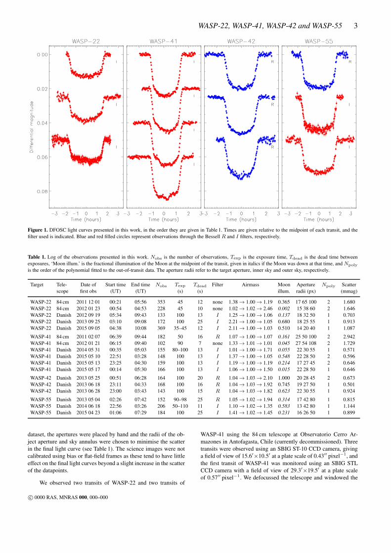
Figure 1. DFOSC light curves presented in this work, in the order they are given in Table 1. Times are given relative to the midpoint of each transit, and the

filter used is indicated. Blue and red filled circles represent observations through the Bessell R and I filters, respectively.

Table 1. Log of the observations presented in this work. Nobs is the number of observations, Texp is the exposure time, Tdead is the dead time between

exposures, ‘Moon illum.’ is the fractional illumination of the Moon at the midpoint of the transit, given in italics if the Moon was down at that time, and Npoly

is the order of the polynomial fitted to the out-of-transit data. The aperture radii refer to the target aperture, inner sky and outer sky, respectively.

Target Tele- Date of Start time End time Nobs Texp Tdead Filter Airmass Moon Aperture Npoly Scatter

scope first obs (UT) (UT) (s) (s) illum. radii (px) (mmag)

WASP-22 84 cm 2011 12 01 00:21 05:56 353 45 12 none 1.38 → 1.00 → 1.19 0.365 17 65 100 2 1.680

WASP-22 84 cm 2012 01 23 00:54 04:53 228 45 10 none 1.02 → 1.02 → 2.46 0.002 15 38 60 2 1.646

WASP-22 Danish 2012 09 19 05:34 09:43 133 100 13 I 1.25 → 1.00 → 1.06 0.137 18 32 50 1 0.703

WASP-22 Danish 2013 09 25 03:10 09:08 172 100 25 I 2.21 → 1.00 → 1.05 0.680 18 25 55 1 0.913

WASP-22 Danish 2015 09 05 04:38 10:08 369 35–45 12 I 2.11 → 1.00 → 1.03 0.510 14 20 40 1 1.087

WASP-41 84 cm 2011 02 07 06:39 09:44 182 50 16 R 1.07 → 1.00 → 1.07 0.161 25 50 100 2 2.942

WASP-41 84 cm 2012 01 21 06:15 09:40 102 90 7 none 1.33 → 1.01 → 1.01 0.045 27 54 108 2 1.729

WASP-41 Danish 2014 05 31 00:35 05:03 155 80–100 13 I 1.01 → 1.00 → 1.71 0.055 22 30 55 1 0.571

WASP-41 Danish 2015 05 10 22:51 03:28 148 100 13 I 1.37 → 1.00 → 1.05 0.548 22 28 50 2 0.596

WASP-41 Danish 2015 05 13 23:25 04:30 159 100 13 I 1.19 → 1.00 → 1.19 0.214 17 27 45 2 0.646

WASP-41 Danish 2015 05 17 00:14 05:30 166 100 13 I 1.06 → 1.00 → 1.50 0.015 22 28 50 1 0.646

WASP-42 Danish 2013 05 25 00:51 06:28 164 100 20 R 1.04 → 1.03 → 2.10 1.000 20 28 45 2 0.673

WASP-42 Danish 2013 06 18 23:11 04:33 168 100 16 R 1.04 → 1.03 → 1.92 0.745 19 27 50 1 0.501

WASP-42 Danish 2013 06 28 23:00 03:43 143 100 15 R 1.04 → 1.03 → 1.82 0.623 22 30 55 1 0.924

WASP-55 Danish 2013 05 04 02:26 07:42 152 90–98 25 R 1.05 → 1.02 → 1.94 0.314 17 42 80 1 0.815

WASP-55 Danish 2014 06 18 22:56 03:26 206 50–110 11 I 1.10 → 1.02 → 1.35 0.583 13 42 80 1 1.144

WASP-55 Danish 2015 04 23 01:06 07:29 184 100 25 I 1.41 → 1.02 → 1.45 0.231 16 26 50 1 0.899

dataset, the apertures were placed by hand and the radii of the ob-

ject aperture and sky annulus were chosen to minimise the scatter

in the final light curve (see Table 1). The science images were not

calibrated using bias or flat-field frames as these tend to have little

effect on the final light curves beyond a slight increase in the scatter

of the datapoints.

We observed two transits of WASP-22 and two transits of

WASP-41 using the 84 cm telescope at Observatorio Cerro Ar-

mazones in Antofagasta, Chile (currently decommissioned). Three

transits were observed using an SBIG ST-10 CCD camera, giving

a field of view of 15.6′×10.5′ at a plate scale of 0.43′′ pixel−1, and

the first transit of WASP-41 was monitored using an SBIG STL

CCD camera with a field of view of 29.3′×19.5′ at a plate scale

of 0.57′′ pixel−1. We defocussed the telescope and windowed the

c© 0000 RAS, MNRAS 000, 000–000

4 Southworth et al.

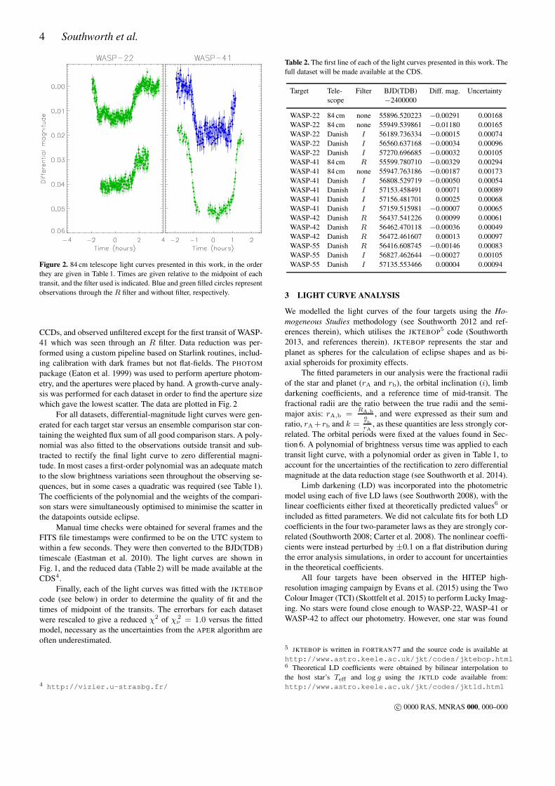
Figure 2. 84 cm telescope light curves presented in this work, in the order

they are given in Table 1. Times are given relative to the midpoint of each

transit, and the filter used is indicated. Blue and green filled circles represent

observations through the R filter and without filter, respectively.

CCDs, and observed unfiltered except for the first transit of WASP-

41 which was seen through an R filter. Data reduction was per-

formed using a custom pipeline based on Starlink routines, includ-

ing calibration with dark frames but not flat-fields. The PHOTOM

package (Eaton et al. 1999) was used to perform aperture photom-

etry, and the apertures were placed by hand. A growth-curve analy-

sis was performed for each dataset in order to find the aperture size

which gave the lowest scatter. The data are plotted in Fig. 2

For all datasets, differential-magnitude light curves were gen-

erated for each target star versus an ensemble comparison star con-

taining the weighted flux sum of all good comparison stars. A poly-

nomial was also fitted to the observations outside transit and sub-

tracted to rectify the final light curve to zero differential magni-

tude. In most cases a first-order polynomial was an adequate match

to the slow brightness variations seen throughout the observing se-

quences, but in some cases a quadratic was required (see Table 1).

The coefficients of the polynomial and the weights of the compari-

son stars were simultaneously optimised to minimise the scatter in

the datapoints outside eclipse.

Manual time checks were obtained for several frames and the

FITS file timestamps were confirmed to be on the UTC system to

within a few seconds. They were then converted to the BJD(TDB)

timescale (Eastman et al. 2010). The light curves are shown in

Fig. 1, and the reduced data (Table 2) will be made available at the

CDS4.

Finally, each of the light curves was fitted with the JKTEBOP

code (see below) in order to determine the quality of fit and the

times of midpoint of the transits. The errorbars for each dataset

were rescaled to give a reduced χ2 of χ 2ν = 1.0 versus the fitted

model, necessary as the uncertainties from the APER algorithm are

often underestimated.

4 http://vizier.u-strasbg.fr/

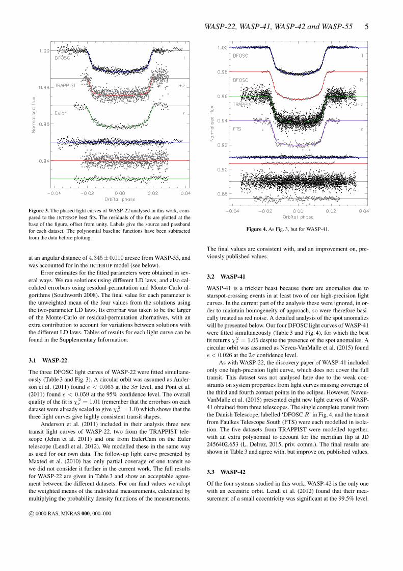
Table 2. The first line of each of the light curves presented in this work. The

full dataset will be made available at the CDS.

Target Tele- Filter BJD(TDB) Diff. mag. Uncertainty

scope −2400000

WASP-22 84 cm none 55896.520223 −0.00291 0.00168

WASP-22 84 cm none 55949.539861 −0.01180 0.00165

WASP-22 Danish I 56189.736334 −0.00015 0.00074

WASP-22 Danish I 56560.637168 −0.00034 0.00096

WASP-22 Danish I 57270.696685 −0.00032 0.00105

WASP-41 84 cm R 55599.780710 −0.00329 0.00294

WASP-41 84 cm none 55947.763186 −0.00187 0.00173

WASP-41 Danish I 56808.529719 −0.00050 0.00054

WASP-41 Danish I 57153.458491 0.00071 0.00089

WASP-41 Danish I 57156.481701 0.00025 0.00068

WASP-41 Danish I 57159.515981 −0.00007 0.00065

WASP-42 Danish R 56437.541226 0.00099 0.00061

WASP-42 Danish R 56462.470118 −0.00036 0.00049

WASP-42 Danish R 56472.461607 0.00013 0.00097

WASP-55 Danish R 56416.608745 −0.00146 0.00083

WASP-55 Danish I 56827.462644 −0.00027 0.00105

WASP-55 Danish I 57135.553466 0.00004 0.00094

3 LIGHT CURVE ANALYSIS

We modelled the light curves of the four targets using the Ho-

mogeneous Studies methodology (see Southworth 2012 and ref-

erences therein), which utilises the JKTEBOP5 code (Southworth

2013, and references therein). JKTEBOP represents the star and

planet as spheres for the calculation of eclipse shapes and as bi-

axial spheroids for proximity effects.

The fitted parameters in our analysis were the fractional radii

of the star and planet (rA and rb), the orbital inclination (i), limb

darkening coefficients, and a reference time of mid-transit. The

fractional radii are the ratio between the true radii and the semi-

major axis: rA,b =RA,b

a, and were expressed as their sum and

ratio, rA+rb and k = rbrA

, as these quantities are less strongly cor-

related. The orbital periods were fixed at the values found in Sec-

tion 6. A polynomial of brightness versus time was applied to each

transit light curve, with a polynomial order as given in Table 1, to

account for the uncertainties of the rectification to zero differential

magnitude at the data reduction stage (see Southworth et al. 2014).

Limb darkening (LD) was incorporated into the photometric

model using each of five LD laws (see Southworth 2008), with the

linear coefficients either fixed at theoretically predicted values6 or

included as fitted parameters. We did not calculate fits for both LD

coefficients in the four two-parameter laws as they are strongly cor-

related (Southworth 2008; Carter et al. 2008). The nonlinear coeffi-

cients were instead perturbed by ±0.1 on a flat distribution during

the error analysis simulations, in order to account for uncertainties

in the theoretical coefficients.

All four targets have been observed in the HITEP high-

resolution imaging campaign by Evans et al. (2015) using the Two

Colour Imager (TCI) (Skottfelt et al. 2015) to perform Lucky Imag-

ing. No stars were found close enough to WASP-22, WASP-41 or

WASP-42 to affect our photometry. However, one star was found

5 JKTEBOP is written in FORTRAN77 and the source code is available at

http://www.astro.keele.ac.uk/jkt/codes/jktebop.html6 Theoretical LD coefficients were obtained by bilinear interpolation to

the host star’s Teff and log g using the JKTLD code available from:

http://www.astro.keele.ac.uk/jkt/codes/jktld.html

c© 0000 RAS, MNRAS 000, 000–000


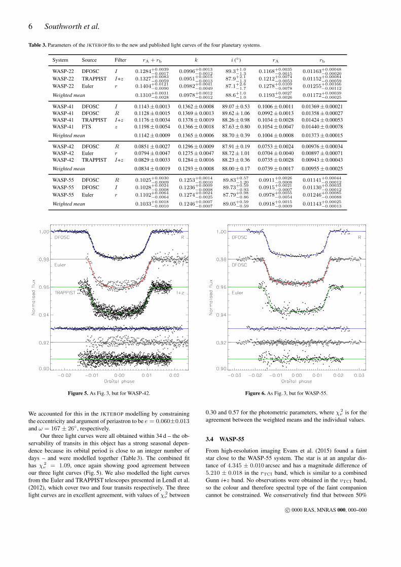
Figure 3. The phased light curves of WASP-22 analysed in this work, com-

pared to the JKTEBOP best fits. The residuals of the fits are plotted at the

base of the figure, offset from unity. Labels give the source and passband

for each dataset. The polynomial baseline functions have been subtracted

from the data before plotting.

at an angular distance of 4.345±0.010 arcsec from WASP-55, and

was accounted for in the JKTEBOP model (see below).

Error estimates for the fitted parameters were obtained in sev-

eral ways. We ran solutions using different LD laws, and also cal-

culated errorbars using residual-permutation and Monte Carlo al-

gorithms (Southworth 2008). The final value for each parameter is

the unweighted mean of the four values from the solutions using

the two-parameter LD laws. Its errorbar was taken to be the larger

of the Monte-Carlo or residual-permutation alternatives, with an

extra contribution to account for variations between solutions with

the different LD laws. Tables of results for each light curve can be

found in the Supplementary Information.

3.1 WASP-22

The three DFOSC light curves of WASP-22 were fitted simultane-

ously (Table 3 and Fig. 3). A circular orbit was assumed as Ander-

son et al. (2011) found e < 0.063 at the 3σ level, and Pont et al.

(2011) found e < 0.059 at the 95% confidence level. The overall

quality of the fit is χ 2ν = 1.01 (remember that the errorbars on each

dataset were already scaled to give χ 2ν = 1.0) which shows that the

three light curves give highly consistent transit shapes.

Anderson et al. (2011) included in their analysis three new

transit light curves of WASP-22, two from the TRAPPIST tele-

scope (Jehin et al. 2011) and one from EulerCam on the Euler

telescope (Lendl et al. 2012). We modelled these in the same way

as used for our own data. The follow-up light curve presented by

Maxted et al. (2010) has only partial coverage of one transit so

we did not consider it further in the current work. The full results

for WASP-22 are given in Table 3 and show an acceptable agree-

ment between the different datasets. For our final values we adopt

the weighted means of the individual measurements, calculated by

multiplying the probability density functions of the measurements.

Figure 4. As Fig. 3, but for WASP-41.

The final values are consistent with, and an improvement on, pre-

viously published values.

3.2 WASP-41

WASP-41 is a trickier beast because there are anomalies due to

starspot-crossing events in at least two of our high-precision light

curves. In the current part of the analysis these were ignored, in or-

der to maintain homogeneity of approach, so were therefore basi-

cally treated as red noise. A detailed analysis of the spot anomalies

will be presented below. Our four DFOSC light curves of WASP-41

were fitted simultaneously (Table 3 and Fig. 4), for which the best

fit returns χ 2ν = 1.05 despite the presence of the spot anomalies. A

circular orbit was assumed as Neveu-VanMalle et al. (2015) found

e < 0.026 at the 2σ confidence level.

As with WASP-22, the discovery paper of WASP-41 included

only one high-precision light curve, which does not cover the full

transit. This dataset was not analysed here due to the weak con-

straints on system properties from light curves missing coverage of

the third and fourth contact points in the eclipse. However, Neveu-

VanMalle et al. (2015) presented eight new light curves of WASP-

41 obtained from three telescopes. The single complete transit from

the Danish Telescope, labelled ‘DFOSC R’ in Fig. 4, and the transit

from Faulkes Telescope South (FTS) were each modelled in isola-

tion. The five datasets from TRAPPIST were modelled together,

with an extra polynomial to account for the meridian flip at JD

2456402.653 (L. Delrez, 2015, priv. comm.). The final results are

shown in Table 3 and agree with, but improve on, published values.

3.3 WASP-42

Of the four systems studied in this work, WASP-42 is the only one

with an eccentric orbit. Lendl et al. (2012) found that their mea-

surement of a small eccentricity was significant at the 99.5% level.

c© 0000 RAS, MNRAS 000, 000–000

6 Southworth et al.

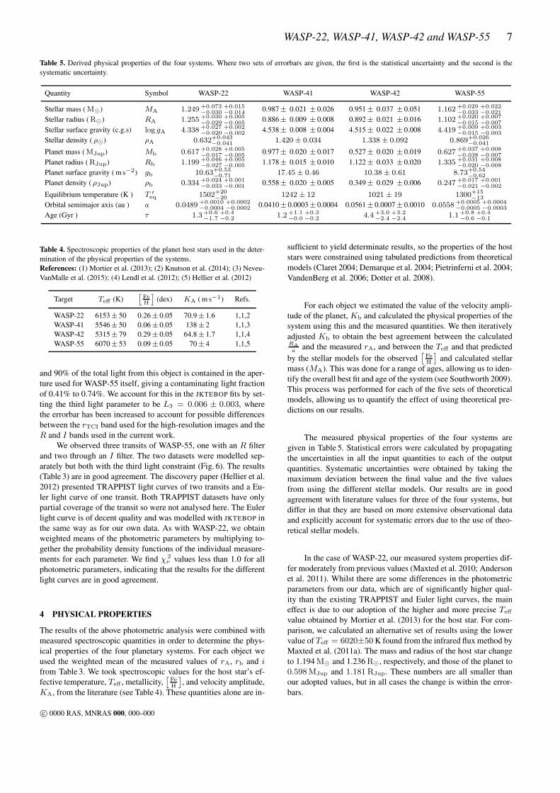
Table 3. Parameters of the JKTEBOP fits to the new and published light curves of the four planetary systems.

System Source Filter rA + rb k i (◦) rA rb

WASP-22 DFOSC I 0.1284+0.0039−0.0017

0.0996+0.0013−0.0012

89.3+1.0−1.3

0.1168+0.0035−0.0015

0.01163+0.00048−0.00020

WASP-22 TRAPPIST I+z 0.1327+0.0083−0.0059 0.0951+0.0015

−0.0013 87.9+2.1−1.3 0.1212+0.0074

−0.0053 0.01152+0.00084−0.00059

WASP-22 Euler r 0.1404+0.0121−0.0090

0.0982+0.0041−0.0049

87.1+2.6−1.7

0.1278+0.0109−0.0078

0.01255+0.00166−0.00112

Weighted mean 0.1310+0.0031−0.0028 0.0978+0.0012

−0.0012 88.6+1.0−1.0 0.1193+0.0027

−0.0026 0.01172+0.00039−0.00025

WASP-41 DFOSC I 0.1143± 0.0013 0.1362± 0.0008 89.07± 0.53 0.1006± 0.0011 0.01369± 0.00021

WASP-41 DFOSC R 0.1128± 0.0015 0.1369± 0.0013 89.62± 1.06 0.0992± 0.0013 0.01358± 0.00027

WASP-41 TRAPPIST I+z 0.1176± 0.0034 0.1378± 0.0019 88.26± 0.98 0.1034± 0.0028 0.01424± 0.00053

WASP-41 FTS z 0.1198± 0.0054 0.1366± 0.0018 87.63± 0.80 0.1054± 0.0047 0.01440± 0.00078

Weighted mean 0.1142± 0.0009 0.1365± 0.0006 88.70± 0.39 0.1004± 0.0008 0.01373± 0.00015

WASP-42 DFOSC R 0.0851± 0.0027 0.1296± 0.0009 87.91± 0.19 0.0753± 0.0024 0.00976± 0.00034

WASP-42 Euler r 0.0794± 0.0047 0.1275± 0.0047 88.72± 1.01 0.0704± 0.0040 0.00897± 0.00071

WASP-42 TRAPPIST I+z 0.0829± 0.0033 0.1284± 0.0016 88.23± 0.36 0.0735± 0.0028 0.00943± 0.00043

Weighted mean 0.0834± 0.0019 0.1293± 0.0008 88.00± 0.17 0.0739± 0.0017 0.00955± 0.00025

WASP-55 DFOSC R 0.1025+0.0030−0.0009 0.1253+0.0014

−0.0010 89.83+0.57−1.20 0.0911+0.0026

−0.0008 0.01141+0.00044−0.00012

WASP-55 DFOSC I 0.1028+0.0024−0.0008

0.1236+0.0009−0.0008

89.73+0.59−0.93

0.0915+0.0021−0.0007

0.01130+0.00033−0.00012

WASP-55 Euler r 0.1102+0.0064−0.0064 0.1274+0.0024

−0.0025 87.79+0.98−0.86 0.0978+0.0055

−0.0054 0.01246+0.00085−0.00088

Weighted mean 0.1033+0.0018−0.0010

0.1246+0.0007−0.0007

89.05+0.59−0.59

0.0918+0.0015−0.0009

0.01143+0.00025−0.00013


We accounted for this in the JKTEBOP modelling by constraining

the eccentricity and argument of periastron to be e = 0.060±0.013and ω = 167 ± 26◦, respectively.

Our three light curves were all obtained within 34 d – the ob-

servability of transits in this object has a strong seasonal depen-

dence because its orbital period is close to an integer number of

days – and were modelled together (Table 3). The combined fit

has χ 2ν = 1.09, once again showing good agreement between

our three light curves (Fig. 5). We also modelled the light curves

from the Euler and TRAPPIST telescopes presented in Lendl et al.

(2012), which cover two and four transits respectively. The three

light curves are in excellent agreement, with values of χ 2ν between


0.30 and 0.57 for the photometric parameters, where χ 2ν is for the

agreement between the weighted means and the individual values.

3.4 WASP-55

From high-resolution imaging Evans et al. (2015) found a faint

star close to the WASP-55 system. The star is at an angular dis-

tance of 4.345 ± 0.010 arcsec and has a magnitude difference of

5.210 ± 0.018 in the rTCI band, which is similar to a combined

Gunn i+z band. No observations were obtained in the vTCI band,

so the colour and therefore spectral type of the faint companion

cannot be constrained. We conservatively find that between 50%

c© 0000 RAS, MNRAS 000, 000–000


Table 5. Derived physical properties of the four systems. Where two sets of errorbars are given, the first is the statistical uncertainty and the second is the

systematic uncertainty.

Quantity Symbol WASP-22 WASP-41 WASP-42 WASP-55

Stellar mass (M⊙) MA 1.249+0.073−0.030

+0.015−0.014 0.987± 0.021 ± 0.026 0.951± 0.037 ± 0.051 1.162+0.029

−0.033+0.022−0.021

Stellar radius (R⊙) RA 1.255+0.030−0.029

+0.005−0.005

0.886± 0.009 ± 0.008 0.892± 0.021 ± 0.016 1.102+0.020−0.015

+0.007−0.007

Stellar surface gravity (c.g.s) log gA 4.338+0.027−0.020

+0.002−0.002 4.538± 0.008 ± 0.004 4.515± 0.022 ± 0.008 4.419+0.009

−0.015+0.003−0.003

Stellar density ( ρ⊙) ρA 0.632+0.043−0.041 1.420± 0.034 1.338 ± 0.092 0.869+0.026

−0.041

Planet mass (MJup) Mb 0.617+0.028−0.017

+0.005−0.005

0.977± 0.020 ± 0.017 0.527± 0.020 ± 0.019 0.627+0.037−0.038

+0.008−0.007

Planet radius (RJup) Rb 1.199+0.046−0.027

+0.005−0.005 1.178± 0.015 ± 0.010 1.122± 0.033 ± 0.020 1.335+0.031

−0.020+0.008−0.008

Planet surface gravity ( m s−2) gb 10.63+0.53−0.71 17.45± 0.46 10.38± 0.61 8.73+0.54

−0.62

Planet density ( ρJup) ρb 0.334+0.024−0.033

+0.001−0.001

0.558± 0.020 ± 0.005 0.349± 0.029 ± 0.006 0.247+0.017−0.021

+0.001−0.002

Equilibrium temperature (K ) T ′eq 1502

+20−20 1242 ± 12 1021 ± 19 1300

+15−13

Orbital semimajor axis (au ) a 0.0489+0.0010−0.0004

+0.0002−0.0002 0.0410± 0.0003± 0.0004 0.0561± 0.0007± 0.0010 0.0558+0.0005

−0.0005+0.0004−0.0003

Age (Gyr ) τ 1.3+0.6−1.7

+0.4−0.2

1.2+1.1−0.0

+0.3−0.2

4.4+3.0−2.4

+3.2−2.4

1.1+0.8−0.6

+0.4−0.1

Table 4. Spectroscopic properties of the planet host stars used in the deter-

mination of the physical properties of the systems.

References: (1) Mortier et al. (2013); (2) Knutson et al. (2014); (3) Neveu-

VanMalle et al. (2015); (4) Lendl et al. (2012); (5) Hellier et al. (2012)

Target Teff (K)[

FeH

]

(dex) KA ( m s−1) Refs.

WASP-22 6153± 50 0.26± 0.05 70.9± 1.6 1,1,2

WASP-41 5546± 50 0.06± 0.05 138± 2 1,1,3

WASP-42 5315± 79 0.29± 0.05 64.8± 1.7 1,1,4

WASP-55 6070± 53 0.09± 0.05 70± 4 1,1,5

and 90% of the total light from this object is contained in the aper-

ture used for WASP-55 itself, giving a contaminating light fraction

of 0.41% to 0.74%. We account for this in the JKTEBOP fits by set-

ting the third light parameter to be L3 = 0.006 ± 0.003, where

the errorbar has been increased to account for possible differences

between the rTCI band used for the high-resolution images and the

R and I bands used in the current work.

We observed three transits of WASP-55, one with an R filter

and two through an I filter. The two datasets were modelled sep-

arately but both with the third light constraint (Fig. 6). The results

(Table 3) are in good agreement. The discovery paper (Hellier et al.

2012) presented TRAPPIST light curves of two transits and a Eu-

ler light curve of one transit. Both TRAPPIST datasets have only

partial coverage of the transit so were not analysed here. The Euler

light curve is of decent quality and was modelled with JKTEBOP in

the same way as for our own data. As with WASP-22, we obtain

weighted means of the photometric parameters by multiplying to-

gether the probability density functions of the individual measure-

ments for each parameter. We find χ 2ν values less than 1.0 for all

photometric parameters, indicating that the results for the different

light curves are in good agreement.

4 PHYSICAL PROPERTIES

The results of the above photometric analysis were combined with

measured spectroscopic quantities in order to determine the phys-

ical properties of the four planetary systems. For each object we

used the weighted mean of the measured values of rA, rb and i

from Table 3. We took spectroscopic values for the host star’s ef-

fective temperature, Teff , metallicity,[

FeH

]

, and velocity amplitude,

KA, from the literature (see Table 4). These quantities alone are in-

sufficient to yield determinate results, so the properties of the host

stars were constrained using tabulated predictions from theoretical

models (Claret 2004; Demarque et al. 2004; Pietrinferni et al. 2004;

VandenBerg et al. 2006; Dotter et al. 2008).

For each object we estimated the value of the velocity ampli-

tude of the planet, Kb and calculated the physical properties of the

system using this and the measured quantities. We then iteratively

adjusted Kb to obtain the best agreement between the calculatedRA

aand the measured rA, and between the Teff and that predicted

by the stellar models for the observed[

FeH

]

and calculated stellar

mass (MA). This was done for a range of ages, allowing us to iden-

tify the overall best fit and age of the system (see Southworth 2009).

This process was performed for each of the five sets of theoretical

models, allowing us to quantify the effect of using theoretical pre-

dictions on our results.

The measured physical properties of the four systems are

given in Table 5. Statistical errors were calculated by propagating

the uncertainties in all the input quantities to each of the output

quantities. Systematic uncertainties were obtained by taking the

maximum deviation between the final value and the five values

from using the different stellar models. Our results are in good

agreement with literature values for three of the four systems, but

differ in that they are based on more extensive observational data

and explicitly account for systematic errors due to the use of theo-

retical stellar models.

In the case of WASP-22, our measured system properties dif-

fer moderately from previous values (Maxted et al. 2010; Anderson

et al. 2011). Whilst there are some differences in the photometric

parameters from our data, which are of significantly higher qual-

ity than the existing TRAPPIST and Euler light curves, the main

effect is due to our adoption of the higher and more precise Teff

value obtained by Mortier et al. (2013) for the host star. For com-

parison, we calculated an alternative set of results using the lower

value of Teff = 6020±50 K found from the infrared flux method by

Maxted et al. (2011a). The mass and radius of the host star change

to 1.194M⊙ and 1.236R⊙, respectively, and those of the planet to

0.598MJup and 1.181 RJup. These numbers are all smaller than

our adopted values, but in all cases the change is within the error-

bars.

c© 0000 RAS, MNRAS 000, 000–000

8 Southworth et al.

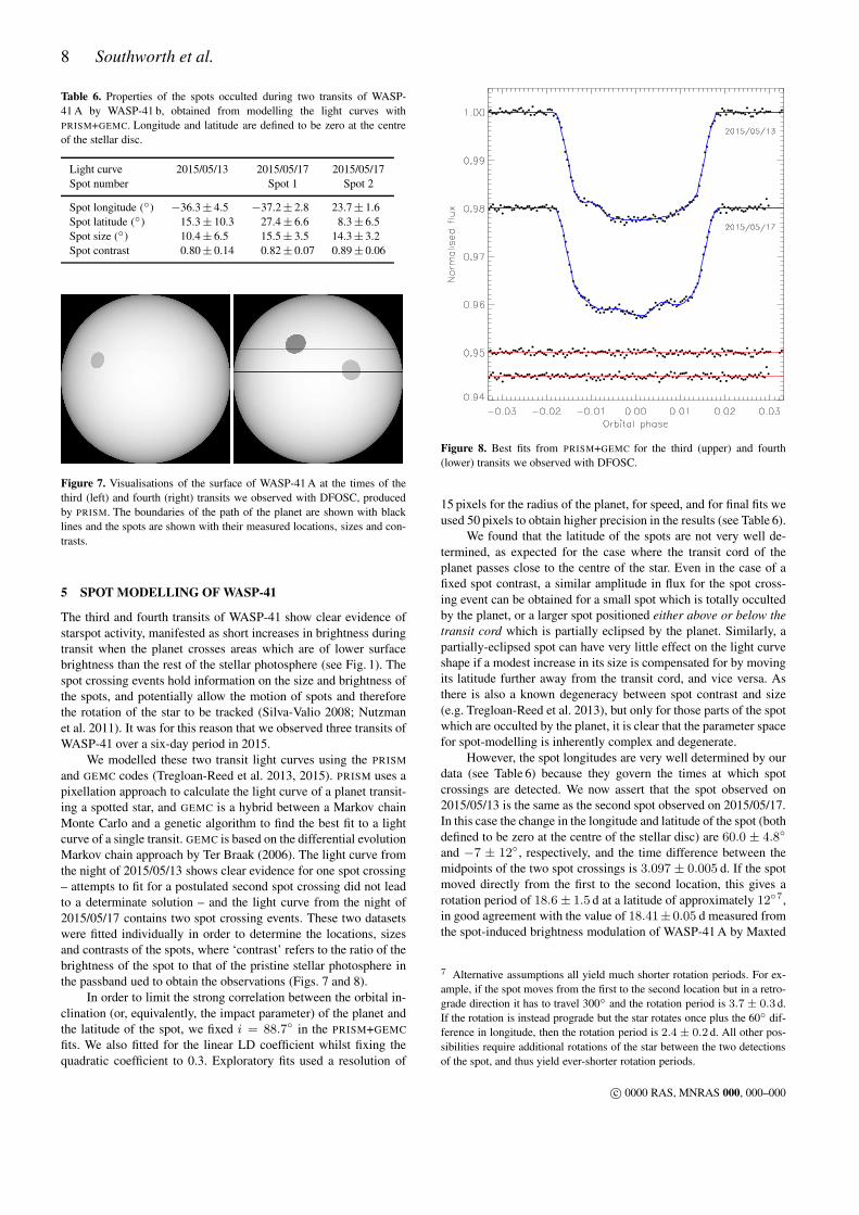
Table 6. Properties of the spots occulted during two transits of WASP-

41 A by WASP-41 b, obtained from modelling the light curves with

PRISM+GEMC. Longitude and latitude are defined to be zero at the centre

of the stellar disc.

Light curve 2015/05/13 2015/05/17 2015/05/17

Spot number Spot 1 Spot 2

Spot longitude (◦) −36.3± 4.5 −37.2± 2.8 23.7± 1.6

Spot latitude (◦) 15.3± 10.3 27.4± 6.6 8.3± 6.5

Spot size (◦) 10.4± 6.5 15.5± 3.5 14.3± 3.2

Spot contrast 0.80± 0.14 0.82± 0.07 0.89± 0.06

Figure 7. Visualisations of the surface of WASP-41 A at the times of the

third (left) and fourth (right) transits we observed with DFOSC, produced

by PRISM. The boundaries of the path of the planet are shown with black

lines and the spots are shown with their measured locations, sizes and con-

trasts.

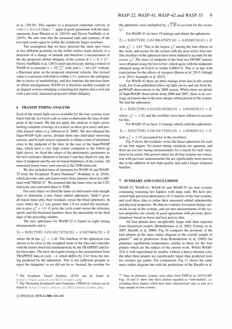
5 SPOT MODELLING OF WASP-41

The third and fourth transits of WASP-41 show clear evidence of

starspot activity, manifested as short increases in brightness during

transit when the planet crosses areas which are of lower surface

brightness than the rest of the stellar photosphere (see Fig. 1). The

spot crossing events hold information on the size and brightness of

the spots, and potentially allow the motion of spots and therefore

the rotation of the star to be tracked (Silva-Valio 2008; Nutzman

et al. 2011). It was for this reason that we observed three transits of

WASP-41 over a six-day period in 2015.

We modelled these two transit light curves using the PRISM

and GEMC codes (Tregloan-Reed et al. 2013, 2015). PRISM uses a

pixellation approach to calculate the light curve of a planet transit-

ing a spotted star, and GEMC is a hybrid between a Markov chain

Monte Carlo and a genetic algorithm to find the best fit to a light

curve of a single transit. GEMC is based on the differential evolution

Markov chain approach by Ter Braak (2006). The light curve from

the night of 2015/05/13 shows clear evidence for one spot crossing

– attempts to fit for a postulated second spot crossing did not lead

to a determinate solution – and the light curve from the night of

2015/05/17 contains two spot crossing events. These two datasets

were fitted individually in order to determine the locations, sizes

and contrasts of the spots, where ‘contrast’ refers to the ratio of the

brightness of the spot to that of the pristine stellar photosphere in

the passband ued to obtain the observations (Figs. 7 and 8).

In order to limit the strong correlation between the orbital in-

clination (or, equivalently, the impact parameter) of the planet and

the latitude of the spot, we fixed i = 88.7◦ in the PRISM+GEMC

fits. We also fitted for the linear LD coefficient whilst fixing the

quadratic coefficient to 0.3. Exploratory fits used a resolution of

Figure 8. Best fits from PRISM+GEMC for the third (upper) and fourth

(lower) transits we observed with DFOSC.

15 pixels for the radius of the planet, for speed, and for final fits we

used 50 pixels to obtain higher precision in the results (see Table 6).

We found that the latitude of the spots are not very well de-

termined, as expected for the case where the transit cord of the

planet passes close to the centre of the star. Even in the case of a

fixed spot contrast, a similar amplitude in flux for the spot cross-

ing event can be obtained for a small spot which is totally occulted

by the planet, or a larger spot positioned either above or below the

transit cord which is partially eclipsed by the planet. Similarly, a

partially-eclipsed spot can have very little effect on the light curve

shape if a modest increase in its size is compensated for by moving

its latitude further away from the transit cord, and vice versa. As

there is also a known degeneracy between spot contrast and size

(e.g. Tregloan-Reed et al. 2013), but only for those parts of the spot

which are occulted by the planet, it is clear that the parameter space

for spot-modelling is inherently complex and degenerate.

However, the spot longitudes are very well determined by our

data (see Table 6) because they govern the times at which spot

crossings are detected. We now assert that the spot observed on

2015/05/13 is the same as the second spot observed on 2015/05/17.

In this case the change in the longitude and latitude of the spot (both

defined to be zero at the centre of the stellar disc) are 60.0 ± 4.8◦

and −7 ± 12◦, respectively, and the time difference between the

midpoints of the two spot crossings is 3.097 ± 0.005 d. If the spot

moved directly from the first to the second location, this gives a

rotation period of 18.6± 1.5 d at a latitude of approximately 12◦7,

in good agreement with the value of 18.41±0.05 d measured from

the spot-induced brightness modulation of WASP-41 A by Maxted

7 Alternative assumptions all yield much shorter rotation periods. For ex-

ample, if the spot moves from the first to the second location but in a retro-

grade direction it has to travel 300◦ and the rotation period is 3.7 ± 0.3 d.

If the rotation is instead prograde but the star rotates once plus the 60◦ dif-

ference in longitude, then the rotation period is 2.4 ± 0.2 d. All other pos-

sibilities require additional rotations of the star between the two detections

of the spot, and thus yield ever-shorter rotation periods.

c© 0000 RAS, MNRAS 000, 000–000


et al. (2011b). This equates to a projected rotational velocity of

v sin i = 2.4± 0.2 km s−1, again in good agreement with the mea-

surements from Maxted et al. (2011b) and Neveu-VanMalle et al.

(2015). We also note that the measured radii and contrasts of the

two spot events agree to within the (relatively large) errorbars.

The assumption that we have detected the same spot twice

in two different positions on the stellar surface leads directly to a

detection of a change of latitude and therefore a measurement of

the sky-projected orbital obliquity of the system of λ = 6 ± 11◦.

Neveu-VanMalle et al. (2015) used spectroscopy during a transit of

WASP-41 to measure λ = 29+10−14

◦ with, and λ = 48±29◦ without,

a Bayesian prior on the projected rotational velocity. Our revised

value is consistent with both to within 1.3σ, removes the ambiguity

due to choice of methodology, and also banishes the previous hints

of orbital misalignment. WASP-41 is therefore another example of

an aligned system containing a transiting hot Jupiter and a cool star

with a precisely measured projected orbital obliquity.

6 TRANSIT TIMING ANALYSIS

Each of the transit light curves available for the four systems were

fitted with the JKTEBOP code in order to determine the time of mid-

point of the transit. We did not apply this analysis to light curves

lacking complete coverage of a transit, as these give noisy and pos-

sibly biased values (e.g. Gibson et al. 2009). We also obtained the

SuperWASP light curves, divided them into individual observing

seasons, and fit each season separately to obtain a time of minimum

close to the midpoint of the data. In the case of the SuperWASP

data, which have a very high scatter compared to the follow-up

light curves, we fixed the values of the photometric parameters to

the best estimates obtained in Section 3 and thus fitted for only the

time of midpoint and the out-of-transit brightness of the system. All

measured transit times were moved to the TDB timescale.

We also included times of minimum for WASP-41 and WASP-

55 from the Exoplanet Transit Database8 (Poddany et al. 2010),

which provides data and transit times from amateur observers affil-

iated with TRESCA9. We assumed that the times were on the UTC

timescale and converted them to TDB.

For each object we fitted the times of mid-transit with straight

lines to determine a new linear orbital ephemeris. Table 7 gives

all transit times plus their residuals versus the fitted ephemeris. In

cases where the χ 2ν was greater than 1.0 we scaled the uncertain-

ties to give χ 2ν = 1.0. E gives the cycle count versus the reference

epoch, and the bracketed numbers show the uncertainty in the final

digit of the preceding number.

The new ephemeris for WASP-22 is based on eight timing

measurements and is:

T0 = BJD(TDB) 2 455 532.72776(22) + 3.53273064(70)×E

where the fit has χ 2ν = 1.46. The timebase of the ephemeris was

chosen to be close to the weighted mean of the data and coincides

with the transit observed simultaneously by the TRAPPIST and Eu-

ler telescopes. The most discrepant timing is the measurement from

TRAPPIST data at cycle −4, which differs by 2.4σ from the tim-

ing predicted by the ephemeris. This is not sufficient grounds to

reject the datapoint, so we did not do so. Instead, the errorbar for

8 The Exoplanet Transit Database (ETD) can be found at:

http://var2.astro.cz/ETD/credit.php9 The TRansiting ExoplanetS and CAndidates (TRESCA) website can be

found at: http://var2.astro.cz/EN/tresca/index.php

the ephemeris were multiplied by√1.46 to account for the excess

χ 2ν .

For WASP-41 we have 19 timings and obtain the ephemeris:

T0 = BJD(TDB) 2 455 996.67927(10) + 3.05240154(41)×E

with χ 2ν = 2.67. This is the largest χ 2

ν among the four objects in

this work, and occurs for the system with the most active host star.

The errorbars of the ephemeris have been inflated to account for the

excess χ 2ν . The times of midpoint of the final two DFOSC transits

were obtained using PRISM+GEMC, which agree with the midpoints

obtained using JKTEBOP to within 0.00015 d. This is in line with

expectations for the effects of starspots (Barros et al. 2013; Oshagh

et al. 2013; Ioannidis et al. 2015)

For WASP-42 there are three timings from data in the current

work, five from published follow-up light curves and one from Su-

perWASP observations in the 2008 season. Whilst there are plenty

of SuperWASP observations from 2006 and 2007, there is no cov-

erage of transits due to the near-integer orbital period of the system.

We find the ephemeris:

T0 = BJD(TDB) 2 455 650.56728(15) + 4.9816819(11) × E

where χ 2ν = 1.35 and the errorbars have been inflated to account

for this.

For WASP-55 we have 11 timings which yield this ephemeris:

T0 = BJD(TDB) 2 456 416.71565(13) + 4.4656291(11) × E

with χ 2ν = 1.10 (accounted for in the errorbars).

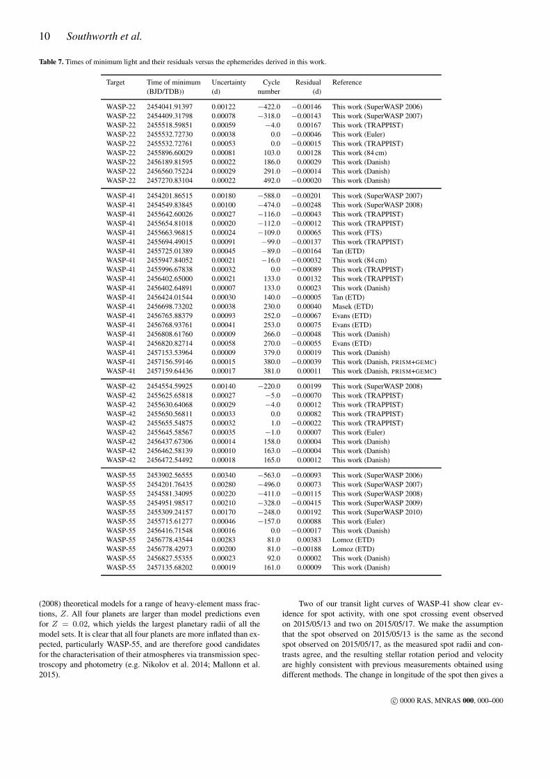
Fig. 9 shows the residuals versus the linear ephemeris for each

of our four targets. No transit timing variations are apparent, and

there are too few timing measurements for a search for such varia-

tions to be useful. Our period values for all four systems are consis-

tent with previous measurements but are significantly more precise

due to the addition of new high-quality data and a longer temporal

baseline.

7 SUMMARY AND CONCLUSIONS

WASP-22, WASP-41, WASP-42 and WASP-55 are four systems

containing transiting hot Jupiters with large radii. We have pre-

sented high-precision photometry of 13 transits of the four systems,

and used these data to refine their measured orbital ephemerides

and physical properties. We find no evidence for transit timing vari-

ations in any of the systems, and our new measurements of the sys-

tem properties are mostly in good agreement with previous deter-

minations based on fewer and less precise data.

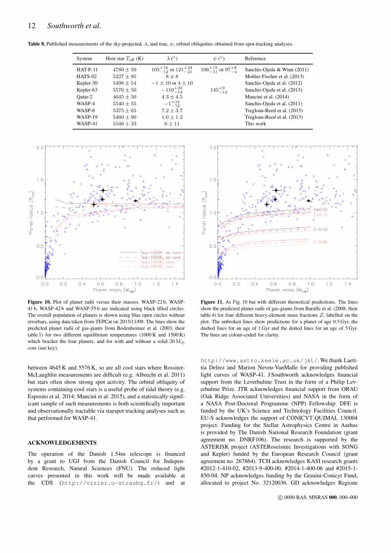
All four planets have inexplicably larger radii than expected

from theoretical models (Bodenheimer et al. 2003; Fortney et al.

2007; Baraffe et al. 2008). Fig. 10 compares the positions of the

four planets in the mass–radius diagram to the overall sample of

planets10 and to predictions from Bodenheimer et al. (2003) for

planetary equilibrium temperatures similar to those for the four

planets which are the subject of the current work. Whilst WASP-

22 b is well represented by models without a heavy-element core,

the other three planets are significantly larger than predicted even

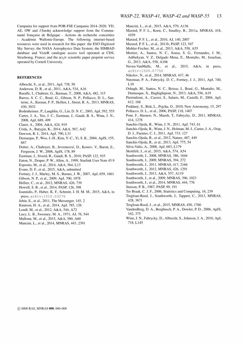
for coreless gas giants. For comparison, Fig. 11 shows the same

mass–radius diagram but with the predictions of the Baraffe et al.

10 Data on planetary systems were taken from TEPCat on 2015/11/09.

Figs. 10 and 11 show only those planets regarded as “well-studied”, i.e.

excluding those planets which have been characterised only as part of a

large sample of such systems.

c© 0000 RAS, MNRAS 000, 000–000

10 Southworth et al.

Table 7. Times of minimum light and their residuals versus the ephemerides derived in this work.

Target Time of minimum Uncertainty Cycle Residual Reference

(BJD/TDB)) (d) number (d)

WASP-22 2454041.91397 0.00122 −422.0 −0.00146 This work (SuperWASP 2006)


WASP-22 2455518.59851 0.00059 −4.0 0.00167 This work (TRAPPIST)

WASP-22 2455532.72730 0.00038 0.0 −0.00046 This work (Euler)

WASP-22 2455532.72761 0.00053 0.0 −0.00015 This work (TRAPPIST)

WASP-22 2455896.60029 0.00081 103.0 0.00128 This work (84 cm)

WASP-22 2456189.81595 0.00022 186.0 0.00029 This work (Danish)

WASP-22 2456560.75224 0.00029 291.0 −0.00014 This work (Danish)




WASP-41 2455642.60026 0.00027 −116.0 −0.00043 This work (TRAPPIST)


WASP-41 2455663.96815 0.00024 −109.0 0.00065 This work (FTS)


WASP-41 2455725.01389 0.00045 −89.0 −0.00164 Tan (ETD)

WASP-41 2455947.84052 0.00021 −16.0 −0.00032 This work (84 cm)


WASP-41 2456402.65000 0.00021 133.0 0.00132 This work (TRAPPIST)


WASP-41 2456424.01544 0.00030 140.0 −0.00005 Tan (ETD)

WASP-41 2456698.73202 0.00038 230.0 0.00040 Masek (ETD)

WASP-41 2456765.88379 0.00093 252.0 −0.00067 Evans (ETD)

WASP-41 2456768.93761 0.00041 253.0 0.00075 Evans (ETD)


WASP-41 2456820.82714 0.00058 270.0 −0.00055 Evans (ETD)


WASP-41 2457156.59146 0.00015 380.0 −0.00039 This work (Danish, PRISM+GEMC)

WASP-41 2457159.64436 0.00017 381.0 0.00011 This work (Danish, PRISM+GEMC)

WASP-42 2454554.59925 0.00140 −220.0 0.00199 This work (SuperWASP 2008)


WASP-42 2455630.64068 0.00029 −4.0 0.00012 This work (TRAPPIST)

WASP-42 2455650.56811 0.00033 0.0 0.00082 This work (TRAPPIST)


WASP-42 2455645.58567 0.00035 −1.0 0.00007 This work (Euler)









WASP-55 2455715.61277 0.00046 −157.0 0.00088 This work (Euler)


WASP-55 2456778.43544 0.00283 81.0 0.00383 Lomoz (ETD)

WASP-55 2456778.42973 0.00200 81.0 −0.00188 Lomoz (ETD)



(2008) theoretical models for a range of heavy-element mass frac-

tions, Z. All four planets are larger than model predictions even

for Z = 0.02, which yields the largest planetary radii of all the

model sets. It is clear that all four planets are more inflated than ex-

pected, particularly WASP-55, and are therefore good candidates

for the characterisation of their atmospheres via transmission spec-

troscopy and photometry (e.g. Nikolov et al. 2014; Mallonn et al.

2015).

Two of our transit light curves of WASP-41 show clear ev-

idence for spot activity, with one spot crossing event observed

on 2015/05/13 and two on 2015/05/17. We make the assumption

that the spot observed on 2015/05/13 is the same as the second

spot observed on 2015/05/17, as the measured spot radii and con-

trasts agree, and the resulting stellar rotation period and velocity

are highly consistent with previous measurements obtained using

different methods. The change in longitude of the spot then gives a

c© 0000 RAS, MNRAS 000, 000–000


Figure 9. Plot of the residuals of the timings of mid-transit versus a linear ephemeris. The results from this work are shown in blue and from amateur observers

in green. Our reanalysis of published data are shown in black for SuperWASP observations and in red for other sources. The grey-shaded regions show the 1σ

uncertainty in the ephemeris as a function of cycle number.

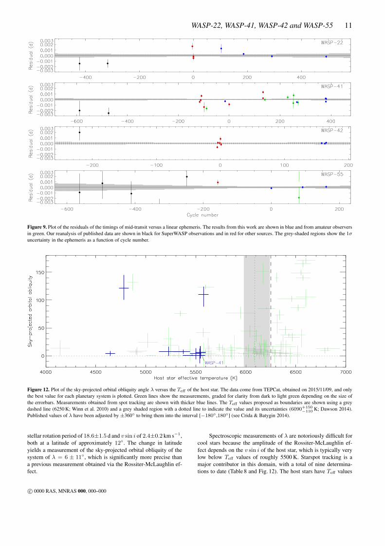
Figure 12. Plot of the sky-projected orbital obliquity angle λ versus the Teff of the host star. The data come from TEPCat, obtained on 2015/11/09, and only

the best value for each planetary system is plotted. Green lines show the measurements, graded for clarity from dark to light green depending on the size of

the errorbars. Measurements obtained from spot tracking are shown with thicker blue lines. The Teff values proposed as boundaries are shown using a grey

dashed line (6250 K; Winn et al. 2010) and a grey shaded region with a dotted line to indicate the value and its uncertainties (6090+150−110

K; Dawson 2014).

Published values of λ have been adjusted by ±360◦ to bring them into the interval [−180◦ ,180◦] (see Crida & Batygin 2014).

stellar rotation period of 18.6±1.5 d and v sin i of 2.4±0.2 km s−1,

both at a latitude of approximately 12◦. The change in latitude

yields a measurement of the sky-projected orbital obliquity of the

system of λ = 6 ± 11◦, which is significantly more precise than

a previous measurement obtained via the Rossiter-McLaughlin ef-

fect.

Spectroscopic measurements of λ are notoriously difficult for

cool stars because the amplitude of the Rossiter-McLaughlin ef-

fect depends on the v sin i of the host star, which is typically very

low below Teff values of roughly 5500 K. Starspot tracking is a

major contributor in this domain, with a total of nine determina-

tions to date (Table 8 and Fig. 12). The host stars have Teff values

c© 0000 RAS, MNRAS 000, 000–000

12 Southworth et al.

Table 8. Published measurements of the sky-projected, λ, and true, ψ, orbital obliquities obtained from spot-tracking analyses.

System Host star Teff (K) λ (◦) ψ (◦) Reference

HAT-P-11 4780 ± 50 105+16−12 or 121+24

−21 106+15−11 or 97+8

−4 Sanchis-Ojeda & Winn (2011)

HATS-02 5227 ± 95 8± 8 Mohler-Fischer et al. (2013)

Kepler-30 5498 ± 54 −1± 10 or 4± 10 Sanchis-Ojeda et al. (2012)

Kepler-63 5576 ± 50 −110+22−14

145+9−14

Sanchis-Ojeda et al. (2013)

Qatar-2 4645 ± 50 4.3± 4.5 Mancini et al. (2014)

WASP-4 5540 ± 55 −1+14−12

Sanchis-Ojeda et al. (2011)

WASP-6 5375 ± 65 7.2± 3.7 Tregloan-Reed et al. (2015)

WASP-19 5460 ± 90 1.0± 1.2 Tregloan-Reed et al. (2013)

WASP-41 5546 ± 33 6± 11 This work

Figure 10. Plot of planet radii versus their masses. WASP-22 b, WASP-

41 b, WASP-42 b and WASP-55 b are indicated using black filled circles.

The overall population of planets is shown using blue open circles without

errorbars, using data taken from TEPCat on 2015/11/09. The lines show the

predicted planet radii of gas-giants from Bodenheimer et al. (2003, their

table 1) for two different equilibrium temperatures (1000 K and 1500 K)

which bracket the four planets, and for with and without a solid 20M⊕

core (see key).

between 4645 K and 5576 K, so are all cool stars where Rossiter-

McLaughlin measurements are difficult (e.g. Albrecht et al. 2011)

but stars often show strong spot activity. The orbital obliquity of

systems containing cool stars is a useful probe of tidal theory (e.g.

Esposito et al. 2014; Mancini et al. 2015), and a statistically signif-

icant sample of such measurements is both scientifically important

and observationally tractable via starspot tracking analyses such as

that performed for WASP-41.

ACKNOWLEDGEMENTS

The operation of the Danish 1.54m telescope is financed

by a grant to UGJ from the Danish Council for Indepen-

dent Research, Natural Sciences (FNU). The reduced light

curves presented in this work will be made available at

the CDS (http://vizier.u-strasbg.fr/) and at

Figure 11. As Fig. 10 but with different theoretical predictions. The lines

show the predicted planet radii of gas-giants from Baraffe et al. (2008, their

table 4) for four different heavy-element mass fractions Z , labelled on the

plot. The unbroken lines show predictions for a planet of age 0.5 Gyr, the

dashed lines for an age of 1 Gyr and the dotted lines for an age of 5 Gyr.

The lines are colour-coded for clarity.

http://www.astro.keele.ac.uk/jkt/. We thank Laeti-

tia Delrez and Marion Neveu-VanMalle for providing published

light curves of WASP-41. J Southworth acknowledges financial

support from the Leverhulme Trust in the form of a Philip Lev-

erhulme Prize. JTR acknowledges financial support from ORAU

(Oak Ridge Associated Universities) and NASA in the form of

a NASA Post-Doctoral Programme (NPP) Fellowship. DFE is

funded by the UK’s Science and Technology Facilities Council.

EU-S acknowledges the support of CONICYT QUIMAL 130004

project. Funding for the Stellar Astrophysics Centre in Aarhus

is provided by The Danish National Research Foundation (grant

agreement no. DNRF106). The research is supported by the

ASTERISK project (ASTERoseismic Investigations with SONG

and Kepler) funded by the European Research Council (grant

agreement no. 267864). TCH acknowledges KASI research grants

#2012-1-410-02, #2013-9-400-00, #2014-1-400-06 and #2015-1-

850-04. NP acknowledges funding by the Gemini-Conicyt Fund,

allocated to project No. 32120036. GD acknowledges Regione

c© 0000 RAS, MNRAS 000, 000–000


Campania for support from POR-FSE Campania 2014–2020. YD,

AE, OW and J Surdej acknowledge support from the Commu-

naute francaise de Belgique - Actions de recherche concertees

- Academie Wallonie-Europe. The following internet-based

resources were used in research for this paper: the ESO Digitized

Sky Survey; the NASA Astrophysics Data System; the SIMBAD

database and VizieR catalogue access tool operated at CDS,

Strasbourg, France; and the arχiv scientific paper preprint service

operated by Cornell University.

REFERENCES

Albrecht, S., et al., 2011, ApJ, 738, 50

Anderson, D. R., et al., 2011, A&A, 534, A16

Baraffe, I., Chabrier, G., Barman, T., 2008, A&A, 482, 315

Barros, S. C. C., Boue, G., Gibson, N. P., Pollacco, D. L., San-

terne, A., Keenan, F. P., Skillen, I., Street, R. A., 2013, MNRAS,

430, 3032

Bodenheimer, P., Laughlin, G., Lin, D. N. C., 2003, ApJ, 592, 555

Carter, J. A., Yee, J. C., Eastman, J., Gaudi, B. S., Winn, J. N.,

2008, ApJ, 689, 499

Claret, A., 2004, A&A, 424, 919

Crida, A., Batygin, K., 2014, A&A, 567, A42

Dawson, R. I., 2014, ApJ, 790, L31

Demarque, P., Woo, J.-H., Kim, Y.-C., Yi, S. K., 2004, ApJS, 155,

667

Dotter, A., Chaboyer, B., Jevremovic, D., Kostov, V., Baron, E.,

Ferguson, J. W., 2008, ApJS, 178, 89

Eastman, J., Siverd, R., Gaudi, B. S., 2010, PASP, 122, 935

Eaton, N., Draper, P. W., Allen, A., 1999, Starlink User Note 45.9

Esposito, M., et al., 2014, A&A, 564, L13

Evans, D. F., et al., 2015, A&A, submitted

Fortney, J. J., Marley, M. S., Barnes, J. W., 2007, ApJ, 659, 1661

Gibson, N. P., et al., 2009, ApJ, 700, 1078

Hellier, C., et al., 2012, MNRAS, 426, 739

Howell, S. B., et al., 2014, PASP, 126, 398

Ioannidis, P., Huber, K. F., Schmitt, J. H. M. M., 2015, A&A, in

press, arXiv:1510.03276

Jehin, E., et al., 2011, The Messenger, 145, 2

Knutson, H. A., et al., 2014, ApJ, 785, 126

Lendl, M., et al., 2012, A&A, 544, A72

Lucy, L. B., Sweeney, M. A., 1971, AJ, 76, 544

Mallonn, M., et al., 2015, A&A, 580, A60

Mancini, L., et al., 2014, MNRAS, 443, 2391

Mancini, L., et al., 2015, A&A, 579, A136

Maxted, P. F. L., Koen, C., Smalley, B., 2011a, MNRAS, 418,

1039

Maxted, P. F. L., et al., 2010, AJ, 140, 2007

Maxted, P. F. L., et al., 2011b, PASP, 123, 547

Mohler-Fischer, M., et al., 2013, A&A, 558, A55

Mortier, A., Santos, N. C., Sousa, S. G., Fernandes, J. M.,

Adibekyan, V. Z., Delgado Mena, E., Montalto, M., Israelian,

G., 2013, A&A, 558, A106

Neveu-VanMalle, M., et al., 2015, A&A, in press,

arXiv:1509.07750

Nikolov, N., et al., 2014, MNRAS, 437, 46

Nutzman, P. A., Fabrycky, D. C., Fortney, J. J., 2011, ApJ, 740,

L10

Oshagh, M., Santos, N. C., Boisse, I., Boue, G., Montalto, M.,

Dumusque, X., Haghighipour, N., 2013, A&A, 556, A19

Pietrinferni, A., Cassisi, S., Salaris, M., Castelli, F., 2004, ApJ,

612, 168

Poddany, S., Brat, L., Pejcha, O., 2010, New Astronomy, 15, 297

Pollacco, D. L., et al., 2006, PASP, 118, 1407

Pont, F., Husnoo, N., Mazeh, T., Fabrycky, D., 2011, MNRAS,

414, 1278

Sanchis-Ojeda, R., Winn, J. N., 2011, ApJ, 743, 61

Sanchis-Ojeda, R., Winn, J. N., Holman, M. J., Carter, J. A., Osip,

D. J., Fuentes, C. I., 2011, ApJ, 733, 127

Sanchis-Ojeda, R., et al., 2012, Nature, 487, 449

Sanchis-Ojeda, R., et al., 2013, ApJ, 775, 54

Silva-Valio, A., 2008, ApJ, 683, L179

Skottfelt, J., et al., 2015, A&A, 574, A54

Southworth, J., 2008, MNRAS, 386, 1644




Southworth, J., 2013, A&A, 557, A119

Southworth, J., et al., 2009, MNRAS, 396, 1023

Southworth, J., et al., 2014, MNRAS, 444, 776

Stetson, P. B., 1987, PASP, 99, 191

Ter Braak, C. J. F., 2006, Statistics and Computing, 16, 239

Tregloan-Reed, J., Southworth, J., Tappert, C., 2013, MNRAS,

428, 3671

Tregloan-Reed, J., et al., 2015, MNRAS, 450, 1760

VandenBerg, D. A., Bergbusch, P. A., Dowler, P. D., 2006, ApJS,

162, 375

Winn, J. N., Fabrycky, D., Albrecht, S., Johnson, J. A., 2010, ApJ,

718, L145

c© 0000 RAS, MNRAS 000, 000–000

High-precision photometry by telescope defocussing. VIII…€¦ · · 2015-12-18High-precision...

Documents

Transcript of High-precision photometry by telescope defocussing. VIII…€¦ · · 2015-12-18High-precision...