Hedging with Options - Jan Römanjanroman.dhis.org/stud/I2008/Hedging/Hedging.pdf · Gamma (Γ)...

School of Education, Culture and Communication Tutor: Jan Röman

Hedging with Options (MMA707)

Authors:

Chiamruchikun Benchaphon 800530-4129 Klongprateepphol Chutima 820708-6722

Pongpala Apiwat 801228-4975 Suntayodom Thanasunun 831224-9264

October 6, 2008 Västerås

CONTENTS

Abstract…………………………………………………………………………. (i)

Introduction…………………………………………………………………….. 1

Definition………………………………………………………………………... 1Hedging……………………………………………………………….…… 1Option……………………………………………………………………… 2

Hedge Parameters……………………………………………………………… 4Delta……………………………………………………………………….. 4Gamma…………………………………………………………………….. 5Theta………………………………………………………………………. 6Vega……………………………………………………………………….. 7Rho………………………………………………………………………… 9

Hedging with Options………………………………………………………….. 9Delta-Hedge……………………………………………………………….. 10Delta-Gamma-Hedge……………………………………………………… 12

Example…………………………………………………………………………. 12

Appendix - Visual Basic Code………………………………………………….. 16

Bibliography……………………………………………………………………. 20

(i)

ABSTRACT

Hedging is a method helping an investor reduces risk in a portfolio. There are many ways under hedging method, one of the most famous methods is hedging by using options as its tool. In this report we introduce you some way how to hedge with option by using delta-hedge and gamma-hedge, moreover we built a VBA application to calculate all important hedging parameters according to our hedging method.

INTRODUCTION

Hedging with option is an investment to reduce or cancel out the risk, from fluctuations in the prices of the securities, by using option to take a position that neutralizes the risk as far as possible. To hedge the portfolio, we have to find the optimal number of securities which make the gain (loss) of the security and option offset each other. In the other word, the gain (loss) on the option position will be offset by the loss (gain) of the security position. To do this, we can use delta and delta-gamma hedge as tools.

In our report, before we understand how to use these tools to reduce the risks, in order to understand deeply we should know some knowledge about option such as option pricing and option factors. So we introduce them in the first part. Next we introduce what the hedging is. After this part the reader can understand how to use option to hedge. Next, we introduce five hedge parameters which are the measure the sensitivity of the option prices with respect to the dependent variables which are stock price (S), time to maturity (T), interest rate (r) and volatility (σ). This part consists of their definition, formulas to calculate and meanings. Then, we introduce how to use delta hedge and delta gamma hedge. The last part, we present the example which we built an application in Visual Basic Application (VBA) to use Black-Scholes to find the optimal hedge for a given number of shares. Moreover, we illustrate using delta and delta-gamma to hedge. We use graphics to show the result of the total portfolio value.

DEFINITION

What is Hedging? (http://www.answers.com/topic/hedging, 29/09/08)

1. Insurance Dictionary Method of transferring Risk to permit the Risk Bearer to assume two offsetting positions at the same time so that, regardless of the outcome of an event, the risk bearer is left in a no win/no lose position. For example, in the options market, a stock owner of an underlying stock can write calls or buy puts. In the same options market, the short sellers of the underlying stock can buy calls or write puts.

2. Britannica Concise Encyclopedia Hedging is a method of reducing the risk of loss caused by price fluctuation. It consists of the purchase or sale of equal quantities of the same or very similar commodities in two different markets at approximately the same time, with the expectation that a future change in price in one market will be offset by an opposite change in the other market. For example, a grain-elevator operator may agree to buy a ton of wheat and at the same time sell a futures contract for the same quantity of wheat; when the wheat is sold, he buys back the futures contract. If the grain price has dropped, he can buy back the futures contract for less than he sold it for; his profit

from doing so will be offset by his loss on the grain. Hedging is also common in the securities and foreign-exchange markets.

3. Columbia Encyclopedia In commerce, method by which traders use two counterbalancing investment strategies so as to minimize any losses caused by price fluctuations. It is generally used by traders on the commodities market. Typically, hedging involves a trader contracting to buy or sell one particular good at the time of the contract and also to buy or sell the same (or similar) commodity at a later date. In a simple example, a miller may buy wheat that is to be converted into flour. At the same time, the miller will contract to sell an equal amount of wheat, which the miller does not presently own, to another trader. The miller agrees to deliver the second lot of wheat at the time the flour is ready for market and at the price current at the time of the agreement. If the price of wheat declines during the period between the miller's purchase of the grain and the flour's entrance onto the market, there will also be a resulting drop in the price of flour. That loss must be sustained by the miller. However, since the miller has a contract to sell wheat at the older, higher price, the miller makes up for this loss on the flour sale by the gain on the wheat sale. Hedging is also employed by stock and bond traders, export-import traders, and some manufacturers.

As you can see from the above, there are many definition of hedging but we can summarize in a short meaning is that hedging is about some methods to reduce the risk that the company face.

What is option?

An option is a contract giving its owner the right to buy or sell an asset at a fixed price on or before a giving date. Options are a unique type of financial contract because they give the buyer the right, but not the obligation, to do something. (Ross, Westerfield, Jaffe, 2005, p.618) There are two types of options, call option and put option.

1. Call Option is a contract gives the holder the right to buy the underlying asset by a certain date (maturity) for a certain price (exercise price).

2. Put Option is a contract gives the holder the right to sell the underlying asset by a certain date for a certain price.

In this report we will scope only in hedging with options especially; how we can use options to hedge. To do this we have to understand more about how to value the option. There are six factors affecting the price of a stock option prices.

- The current price of the underlying asset, which for stock option is the price of a share of common stock. 0S

- The exercise price. K - The time to expiration date. t - The volatility of the underlying asset. σ

The risk-free interest rate. r - The dividends expected during the life of the option. q

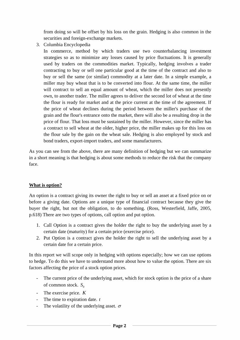
The table below shows the effect of each factor to the value of each type of option.

Variable European call

European put

+ -- +? ?+ ++ -- +

+ indicates that an increase in the variable causes the option price to increase.- indicates that an increase in the variable causes the option price to decrease.? Indicates that the relationship is uncertain.

Risk-free rateAmount of future dividends

Summary of the effect on the price of a stock option of increasing one variable while keeping all others fixed.

Current stock priceStrike priceTime to expirationVolatility

(John C. Hull, p.206)

One of the most famous formulas to valuation the option is Black-Scholes model. It shows us that the value of the option is the function of such factors. The Black-Scholes model is as follow:-

20

1ln( / ) ( / 2)S K r q Td

Tσ

σ+ − + ×

=

20

2ln( / ) ( / 2)S K r q Td

Tσ

σ+ − − ×

=

0 1 2( ) ( )qT rTc S e N d Ke N d− −= −

2 0 1( ) ( )rT qTp Ke N d S e N d− −= − − −

(http://finance.bi.no/~bernt/gcc_prog/recipes/recipes/node9.html, 16/05/08)

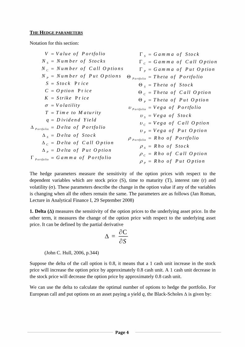
THE HEDGE PARAMETERS

Notation for this section:

P r P r

P r

S

C

P

P o r t fo l io

V V a lu e o f P o r t fo l ioN N u m b e r o f S to c k sN N u m b e r o f C a l l O p t io n sN N u m b e r o f P u t O p t io n s

S S to c k ic eC O p tio n ic eK S tr ik e ic e

V o la t i l i tyT T im e to M a tu r i tyq D iv id e n d Y ie ld

D e l ta o f P o r t f

σ

==

========

Δ =

S

C

P

P o r t fo l io

o l io

D e l ta o f S to c kD e l ta o f C a l l O p t io nD e l ta o f P u t O p t io nG a m m a o f P o r t fo l io

Δ =Δ =Δ =

Γ =

S

C

P

P o r tfo l io

S

C

P

P o r tfo l io

S

C

G a m m a o f S to c kG a m m a o f C a l l O p tio nG a m m a o f P u t O p t io nT h e ta o f P o r t fo l io

T h e ta o f S to c kT h e ta o f C a l l O p t io nT h e ta o f P u t O p t io nV e g a o f P o r t fo l io

V e g a o f S to c k

υ

υυ

Γ =

Γ =

Γ =Θ =

Θ =

Θ =

Θ ==

=

=

P

P o r tfo l io

S

C

P

V e g a o f C a l l O p t io nV e g a o f P u t O p t io nR h o o f P o r t fo l io

R h o o f S to c kR h o o f C a l l O p t io nR h o o f P u t O p t io n

υρ

ρρρ

==

=

=

=

The hedge parameters measure the sensitivity of the option prices with respect to the dependent variables which are stock price (S), time to maturity (T), interest rate (r) and volatility (σ). These parameters describe the change in the option value if any of the variables is changing when all the others remain the same. The parameters are as follows (Jan Roman, Lecture in Analytical Finance I, 29 September 2008)

1. Delta (Δ) measures the sensitivity of the option prices to the underlying asset price. In the other term, it measures the change of the option price with respect to the underlying asset price. It can be defined by the partial derivative

C= S

∂Δ

∂

(John C. Hull, 2006, p.344)

Suppose the delta of the call option is 0.8, it means that a 1 cash unit increase in the stock price will increase the option price by approximately 0.8 cash unit. A 1 cash unit decrease in the stock price will decrease the option price by approximately 0.8 cash unit.

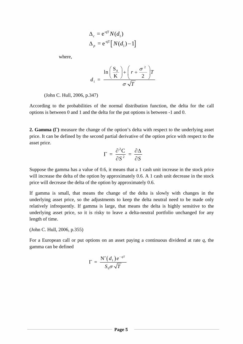
We can use the delta to calculate the optimal number of options to hedge the portfolio. For European call and put options on an asset paying a yield q, the Black-Scholes Δ is given by:

[ ]

-qT1

-qT1

= e ( )

= e ( ) 1c

p

N d

N d

Δ

Δ −

where,

20

1

SlnK 2

= r T

dT

σ

σ

⎛ ⎞⎛ ⎞ + +⎜ ⎟⎜ ⎟⎝ ⎠ ⎝ ⎠

(John C. Hull, 2006, p.347)

According to the probabilities of the normal distribution function, the delta for the call options is between 0 and 1 and the delta for the put options is between -1 and 0.

2. Gamma (Γ) measure the change of the option’s delta with respect to the underlying asset price. It can be defined by the second partial derivative of the option price with respect to the asset price.

2

2

C= = S S

∂ ∂ΔΓ

∂ ∂

Suppose the gamma has a value of 0.6, it means that a 1 cash unit increase in the stock price will increase the delta of the option by approximately 0.6. A 1 cash unit decrease in the stock price will decrease the delta of the option by approximately 0.6.

If gamma is small, that means the change of the delta is slowly with changes in the underlying asset price, so the adjustments to keep the delta neutral need to be made only relatively infrequently. If gamma is large, that means the delta is highly sensitive to the underlying asset price, so it is risky to leave a delta-neutral portfolio unchanged for any length of time.

(John C. Hull, 2006, p.355)

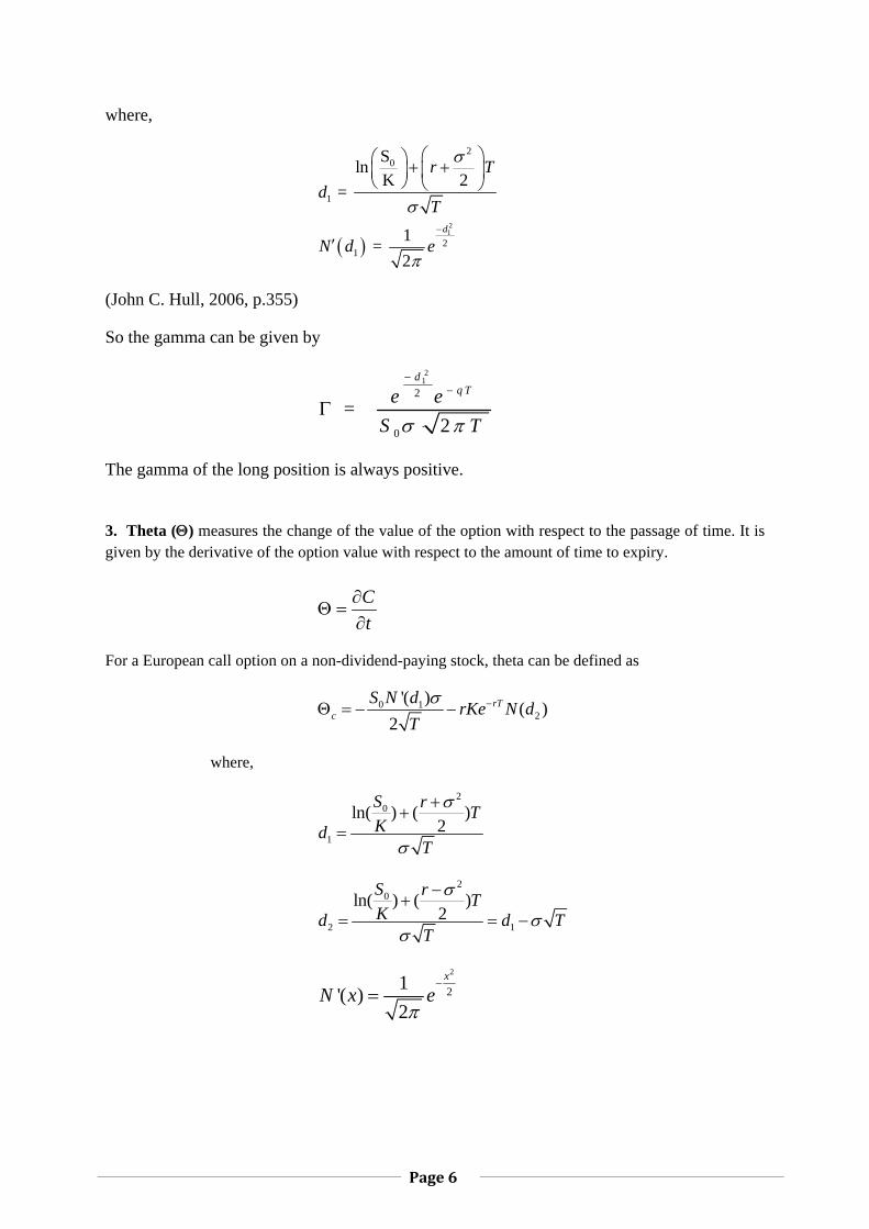
For a European call or put options on an asset paying a continuous dividend at rate q, the gamma can be defined

( )1

0

N =

qTd eS Tσ

−′Γ

where,

( )21

20

1

21

SlnK 2

=

1 = 2

d

r Td

T

N d e

σ

σ

π

−

⎛ ⎞⎛ ⎞ + +⎜ ⎟⎜ ⎟⎝ ⎠ ⎝ ⎠

′

(John C. Hull, 2006, p.355)

So the gamma can be given by

21

2

0

= 2

dq Te e

S Tσ π

−−

Γ

The gamma of the long position is always positive.

3. Theta (Θ) measures the change of the value of the option with respect to the passage of time. It is given by the derivative of the option value with respect to the amount of time to expiry.

Ct

∂Θ =

∂

For a European call option on a non-dividend-paying stock, theta can be defined as

0 12

'( ) ( )2

rTc

S N d rKe N dT

σ −Θ = − −

where,

20

1

ln( ) ( )2

S r TKd

T

σ

σ

++

=

20

2 1

ln( ) ( )2

S r TKd d T

T

σ

σσ

−+

= = −

2

21'( )2

x

N x eπ

−=

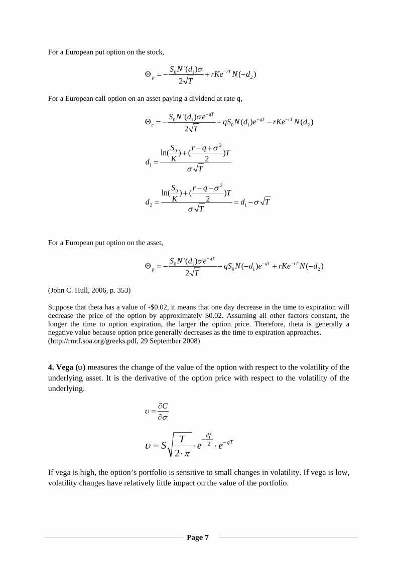
For a European put option on the stock,

0 12

'( ) ( )2

rTp

S N d rKe N dT

σ −Θ = − + −

For a European call option on an asset paying a dividend at rate q,

0 10 1 2

'( ) ( ) ( )2

qTqT rT

cS N d e qS N d e rKe N d

Tσ −

− −Θ = − + −

20

1

ln( ) ( )2

S r q TKd

T

σ

σ

− ++

=

20

2 1

ln( ) ( )2

S r q TKd d T

T

σ

σσ

− −+

= = −

For a European put option on the asset,

0 10 1 2

'( ) ( ) ( )2

qTqT rT

pS N d e qS N d e rKe N d

Tσ −

− −Θ = − − − + −

(John C. Hull, 2006, p. 353) Suppose that theta has a value of -$0.02, it means that one day decrease in the time to expiration will decrease the price of the option by approximately $0.02. Assuming all other factors constant, the longer the time to option expiration, the larger the option price. Therefore, theta is generally a negative value because option price generally decreases as the time to expiration approaches. (http://rmtf.soa.org/greeks.pdf, 29 September 2008) 4. Vega (υ) measures the change of the value of the option with respect to the volatility of the underlying asset. It is the derivative of the option price with respect to the volatility of the underlying.

Cυσ∂

=∂

212

2

dqTTS e eυ

π− −= ⋅ ⋅

⋅

If vega is high, the option’s portfolio is sensitive to small changes in volatility. If vega is low, volatility changes have relatively little impact on the value of the portfolio.

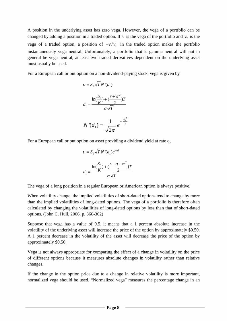
A position in the underlying asset has zero vega. However, the vega of a portfolio can be changed by adding a position in a traded option. If v is the vega of the portfolio and Tv is the

vega of a traded option, a position of / Tv v− in the traded option makes the portfolio instantaneously vega neutral. Unfortunately, a portfolio that is gamma neutral will not in general be vega neutral, at least two traded derivatives dependent on the underlying asset must usually be used.

For a European call or put option on a non-dividend-paying stock, vega is given by

0 1'( )S T N dυ =

20

1

ln( ) ( )2

S r TKd

T

σ

σ

++

=

212

11'( )2

d

N d eπ

−=

For a European call or put option on asset providing a dividend yield at rate q,

0 1'( ) qTS T N d eυ −=

20

1

ln( ) ( )2

S r q TKd

T

σ

σ

− ++

=

The vega of a long position in a regular European or American option is always positive.

When volatility change, the implied volatilities of short-dated options tend to change by more than the implied volatilities of long-dated options. The vega of a portfolio is therefore often calculated by changing the volatilities of long-dated options by less than that of short-dated options. (John C. Hull, 2006, p. 360-362)

Suppose that vega has a value of 0.5, it means that a 1 percent absolute increase in the volatility of the underlying asset will increase the price of the option by approximately $0.50. A 1 percent decrease in the volatility of the asset will decrease the price of the option by approximately $0.50.

Vega is not always appropriate for comparing the effect of a change in volatility on the price of different options because it measures absolute changes in volatility rather than relative changes.

If the change in the option price due to a change in relative volatility is more important, normalized vega should be used. “Normalized vega” measures the percentage change in an

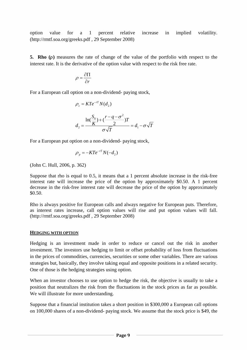
option value for a 1 percent relative increase in implied volatility. (http://rmtf.soa.org/greeks.pdf , 29 September 2008)

5. Rho (ρ) measures the rate of change of the value of the portfolio with respect to the interest rate. It is the derivative of the option value with respect to the risk free rate.

r

ρ ∂Π=∂

For a European call option on a non-dividend- paying stock,

2( )rTc KTe N dρ −=

20

2 1

ln( ) ( )2

S r q TKd d T

T

σ

σσ

− −+

= = −

For a European put option on a non-dividend- paying stock,

2( )rTp KTe N dρ −= − −

(John C. Hull, 2006, p. 362)

Suppose that rho is equal to 0.5, it means that a 1 percent absolute increase in the risk-free interest rate will increase the price of the option by approximately $0.50. A 1 percent decrease in the risk-free interest rate will decrease the price of the option by approximately $0.50. Rho is always positive for European calls and always negative for European puts. Therefore, as interest rates increase, call option values will rise and put option values will fall. (http://rmtf.soa.org/greeks.pdf , 29 September 2008)

HEDGING WITH OPTION

Hedging is an investment made in order to reduce or cancel out the risk in another investment. The investors use hedging to limit or offset probability of loss from fluctuations in the prices of commodities, currencies, securities or some other variables. There are various strategies but, basically, they involve taking equal and opposite positions in a related security. One of those is the hedging strategies using option.

When an investor chooses to use option to hedge the risk, the objective is usually to take a position that neutralizes the risk from the fluctuations in the stock prices as far as possible. We will illustrate for more understanding.

Suppose that a financial institution takes a short position in $300,000 a European call options on 100,000 shares of a non-dividend- paying stock. We assume that the stock price is $49, the

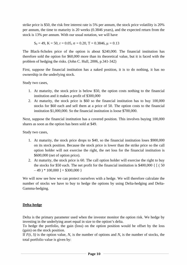
strike price is $50, the risk free interest rate is 5% per annum, the stock price volatility is 20% per annum, the time to maturity is 20 weeks (0.3846 years), and the expected return from the stock is 13% per annum. With our usual notation, we will have

S0 = 49, K = 50, r = 0.05, σ = 0.20, T = 0.3846, μ = 0.13

The Black-Scholes price of the option is about $240,000. The financial institution has therefore sold the option for $60,000 more than its theoretical value, but it is faced with the problem of hedging the risks. (John C. Hull, 2006, p.341-342)

First, suppose the financial institution has a naked position, it is to do nothing, it has no ownership in the underlying stock.

Study two cases,

1. At maturity, the stock price is below $50, the option costs nothing to the financial institution and it makes a profit of $300,000

2. At maturity, the stock price is $60 so the financial institution has to buy 100,000 stocks for $60 each and sell them at a price of 50. The option costs to the financial institution $1,000,000. So the financial institution is loose $700,000.

Next, suppose the financial institution has a covered position. This involves buying 100,000 shares as soon as the option has been sold at $49.

Study two cases,

1. At maturity, the stock price drops to $40, so the financial institution loses $900,000 on its stock position. Because the stock price is lower than the strike price so the call option holder will not exercise the right, the net loss for the financial institution is $600,000 (net of option price).

2. At maturity, the stock price is 60. The call option holder will exercise the right to buy the stocks for $50 each. The net profit for the financial institution is $400,000 { [ ( 50 – 49 ) * 100,000 ] + $300,000 }

We will now see how we can protect ourselves with a hedge. We will therefore calculate the number of stocks we have to buy to hedge the options by using Delta-hedging and Delta- Gamma-hedging.

Delta-hedge

Delta is the primary parameter used when the investor monitor the option risk. We hedge by investing in the underlying asset equal in size to the option’s delta. To hedge the portfolio, the gain (loss) on the option position would be offset by the loss (gain) on the stock position. If F(t, S) is the option value, Nc is the number of options and Ns is the number of stocks, the total portfolio value is given by:

( )

( ) ( )1 1

= , with a delta hedge:

( , ) = +

( , ) = 0, = =

=

= =

c s

c s

s c c c

sc

c

sc

c

V N F t S N S

V F t S SN NS S SdV F t SN N NdS S

NN

NN d N dN

− +

∂ ∂ ∂−

∂ ∂ ∂∂

⇒ Δ∂

Δ

Δ ⇒

∵

∵

The delta for the call options is always positive. Using delta hedging for a short position in a European call option involves keeping a long position in the underlying asset at any given time. Similarly, using delta hedging for a long position in a European call option involves maintaining a short position in the underlying asset at any given time.

The delta for the put options is always negative, which means that a long position in a European put option should be hedged with a long position in the underlying asset, and a short position in a European put option should be hedged with a short position in the underlying asset.

(John C. Hull, 2006, p.346)

From the above example,

( ) ( )

( )

2 20

1

1

1

S 49 0.2ln ln 0.05 0.3846K 2 50 2

= = = 0.05420.2 0.3846

= 0.0542 = 0.52161

so we need = = 0.52161 100,000 =

s c

r Td

T

N d N

N N d N

σ

σ

⎛ ⎞ ⎛ ⎞⎛ ⎞ ⎛ ⎞+ + + +⎜ ⎟⎜ ⎟ ⎜ ⎟⎜ ⎟⎝ ⎠⎝ ⎠ ⎝ ⎠ ⎝ ⎠

∗

∗52,161 stocks to hedge the options

It is important to realize that, because delta changes, the investor’s position remains delta hedged for only a relatively short period of time. So the hedge has to be adjusted periodically.

(John C. Hull, 2006, p.345)

Delta-Gamma-Hedge

In this part, we are talking about how to apply delta-gamma for hedging stock. The sense of this method is about neutralΓ− and neutralΔ− . The value of the hedging portfolio is equal to:-

( , ) ( , )s c c p pV N S N F t S N F t S= ⋅ − ⋅ + ⋅

To make the portfolio Γand Δbe neutral, we give the first and second derivatives of the value of the portfolio with respect to Asset price equal to zero.

2

2 0V VS S∂ ∂

= =∂ ∂

Since 0PortfolioΓ = , we have to use one more option to remove the sensitivity in Δ . Then we have:

0

0Portfolio S C C P P

Portfolio S C C P P

S N N

S N N

Δ = Δ ⋅ −Δ ⋅ + Δ ⋅ =⎧⎪⎨Γ = Γ ⋅ −Γ ⋅ +Γ ⋅ =⎪⎩

We know that 0sΓ = and 1sΔ = then we have:

00

C C P P

P P C C

S N NN N

−Δ ⋅ + Δ ⋅ =⎧⎨Γ ⋅ −Γ ⋅ =⎩

By solving these two equations we can find the number of Call and Put options as:

S PC

P C C P

S CP

P C C P

NN

NN

⋅Γ=Γ ⋅Δ −Γ ⋅Δ

⋅Γ=Γ ⋅Δ −Γ ⋅Δ

The above is the way using delta-gamma-hedge to reduce the risk in our portfolio. For more understanding please see the example in Visual Basis part.

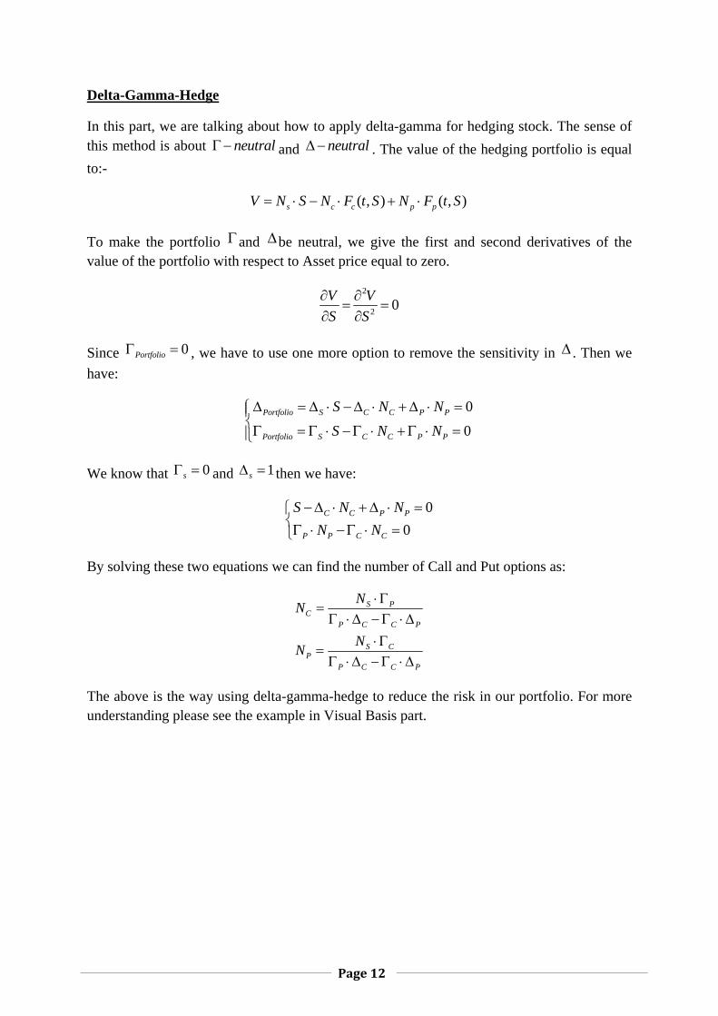
EXAMPLE ( John C. Hull, p.341)

A financial institution has sold a European call option on 100,000 shares of a non-dividend-paying stock for $300,000. Assume that the stock price is $49, the strike price is $50, the risk-free interest rate is 5% per annum, the stock price volatility is 20% per annum and the time to maturity is 20 weeks (0.3846 years). We can summarize as:

0 49500.3846

SKT

===

0.050.20.13

rσμ

===

(For delta-gamma-hedge, we introduce a put option for such stock with strike price at $47.)

We calculate the hedge parameters by using VBA application, Delta Hedging. Firstly, we have to fill our data in the Input box in the application, shown as follow.

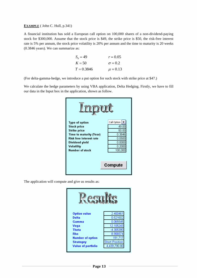
The application will compute and give us results as:

The option price for this option is equal to $2.400461. The sensitivity of the option prices to the underlying asset price is 0.5216. This means when the asset price changes by one unit of dollar the call price will change by 0.5216, in the same way. Next, the change of the option’s delta with respect to the underlying asset price is 0.0655, making us know that the speed of change in options compare with the change in its underlying asset is quite slow. For vega equals 12.1052, means increasing in 1% (or 0.01) of volatility of the underlying asset will be effected to the increasing of this call option price $0.1211. The next parameter is theta from the application this option theta is -4.3054 per year or -0.0118(-4.3054 divided by 365) per calendar day. The meaning is that 1 day decrease in the time to expiration will decrease the price of the option by approximately $0.0118. The last parameter we calculate is rho which is equal to 8.9066. It means that the change in 1% (or 0.01) of interest rate will make the call price change by $0.0891.

Now consider the number of call options we have to make contract to hedge the 100,000 stocks, the result tell us to short 191,717 call options. Doing so will make the portfolio value equal to $4,439,790.80.

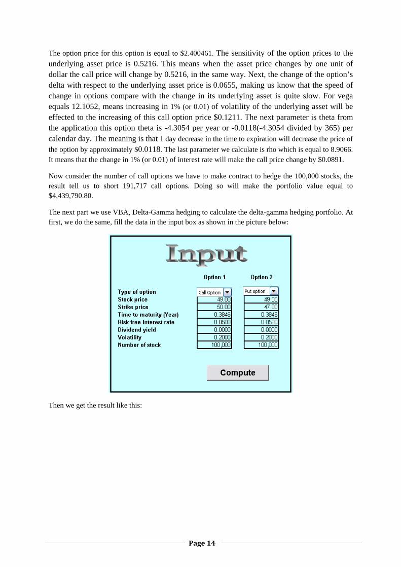
The next part we use VBA, Delta-Gamma hedging to calculate the delta-gamma hedging portfolio. At first, we do the same, fill the data in the input box as shown in the picture below:

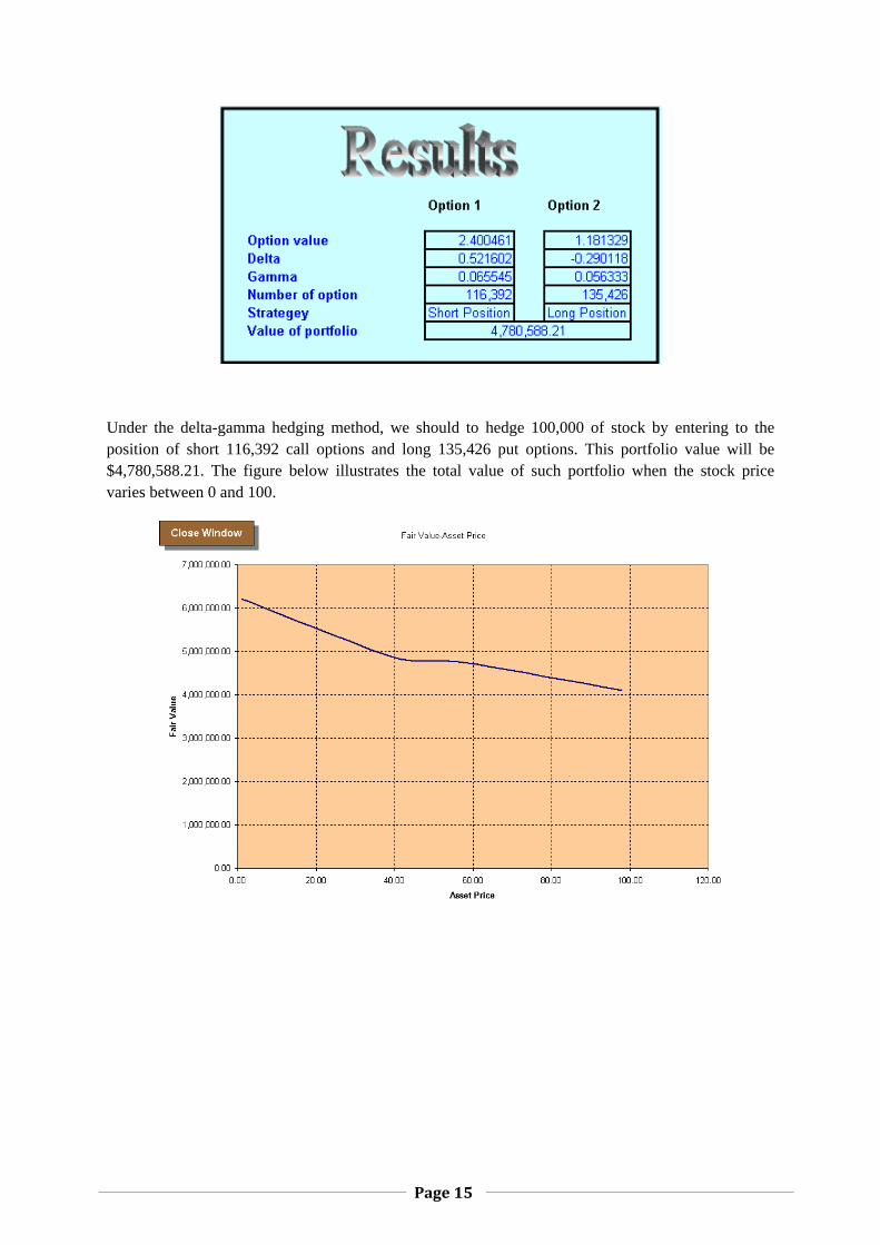
Then we get the result like this:

Under the delta-gamma hedging method, we should to hedge 100,000 of stock by entering to the position of short 116,392 call options and long 135,426 put options. This portfolio value will be $4,780,588.21. The figure below illustrates the total value of such portfolio when the stock price varies between 0 and 100.

APPENDIX

VBA Code

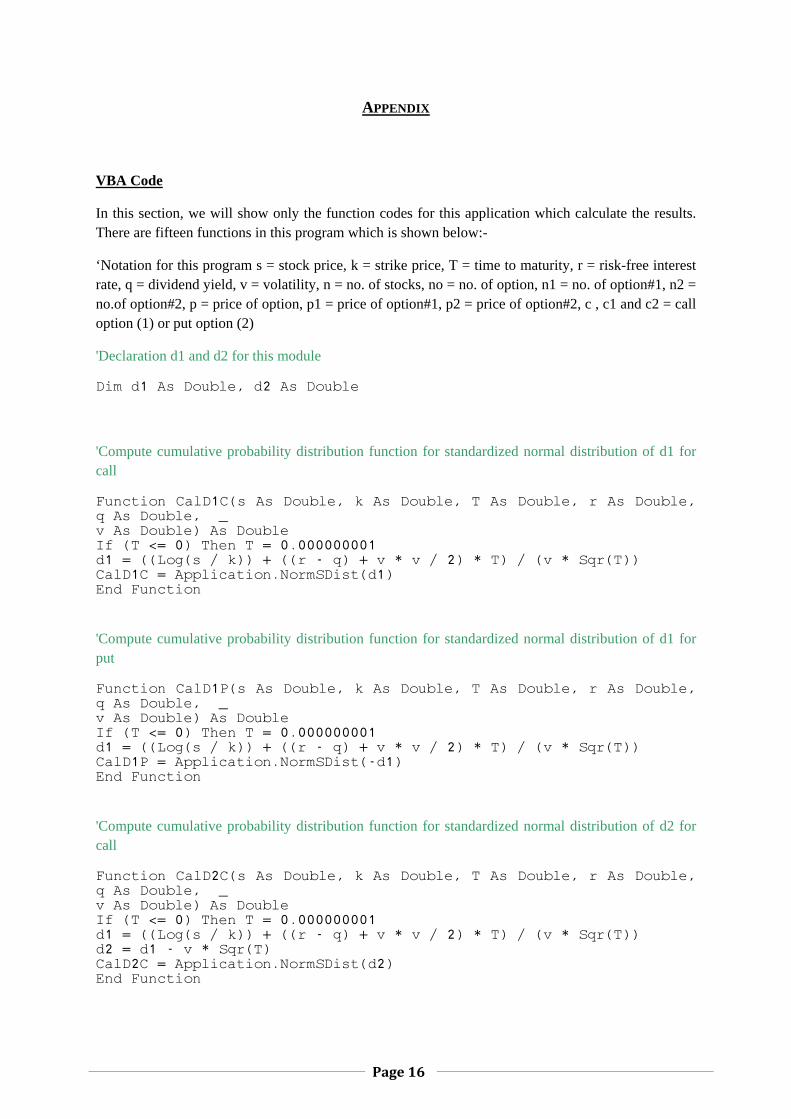
In this section, we will show only the function codes for this application which calculate the results. There are fifteen functions in this program which is shown below:-

‘Notation for this program s = stock price, k = strike price, T = time to maturity, r = risk-free interest rate, q = dividend yield, v = volatility, n = no. of stocks, no = no. of option, n1 = no. of option#1, n2 = no.of option#2, p = price of option, p1 = price of option#1, p2 = price of option#2, c , c1 and c2 = call option (1) or put option (2)

'Declaration d1 and d2 for this module

Dim d1 As Double, d2 As Double

'Compute cumulative probability distribution function for standardized normal distribution of d1 for call

Function CalD1C(s As Double, k As Double, T As Double, r As Double, q As Double, _ v As Double) As Double If (T <= 0) Then T = 0.000000001 d1 = ((Log(s / k)) + ((r - q) + v * v / 2) * T) / (v * Sqr(T)) CalD1C = Application.NormSDist(d1) End Function

'Compute cumulative probability distribution function for standardized normal distribution of d1 for put

Function CalD1P(s As Double, k As Double, T As Double, r As Double, q As Double, _ v As Double) As Double If (T <= 0) Then T = 0.000000001 d1 = ((Log(s / k)) + ((r - q) + v * v / 2) * T) / (v * Sqr(T)) CalD1P = Application.NormSDist(-d1) End Function

'Compute cumulative probability distribution function for standardized normal distribution of d2 for call

Function CalD2C(s As Double, k As Double, T As Double, r As Double, q As Double, _ v As Double) As Double If (T <= 0) Then T = 0.000000001 d1 = ((Log(s / k)) + ((r - q) + v * v / 2) * T) / (v * Sqr(T)) d2 = d1 - v * Sqr(T) CalD2C = Application.NormSDist(d2) End Function

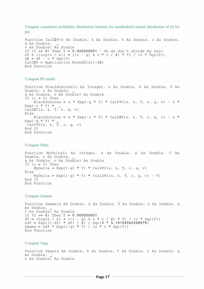
'Compute cumulative probability distribution function for standardized normal distribution of d2 for put

Function CalD2P(s As Double, k As Double, T As Double, r As Double, q As Double, _ v As Double) As Double If (T <= 0) Then T = 0.000000001 ' So we don't divide by zero d1 = ((Log(s / k)) + ((r - q) + v * v / 2) * T) / (v * Sqr(T)) d2 = d1 - v * Sqr(T) CalD2P = Application.NormSDist(-d2) End Function

'Compute BS model

Function BlackScholes(c As Integer, s As Double, k As Double, T As Double, r As Double, _ q As Double, v As Double) As Double If (c = 1) Then BlackScholes = s * Exp(-q * T) * CalD1C(s, k, T, r, q, v) - k * Exp(-r * T) * _ CalD2C(s, k, T, r, q, v) Else BlackScholes = k * Exp(-r * T) * CalD2P(s, k, T, r, q, v) - s * Exp(-q * T) * _ CalD1P(s, k, T, r, q, v) End If End Function

'Compute Delta

Function MyDelta(c As Integer, s As Double, k As Double, T As Double, r As Double, _ q As Double, v As Double) As Double If (c = 1) Then MyDelta = Exp((-q) * T) * CalD1C(s, k, T, r, q, v) Else MyDelta = Exp((-q) * T) * (CalD1C(s, k, T, r, q, v) - 1) End If End Function

'Compute Gamma

Function Gamma(s As Double, k As Double, T As Double, r As Double, q As Double, _ v As Double) As Double If (T <= 0) Then T = 0.000000001 d1 = (Log(s / k) + ((r - q) + v * v / 2) * T) / (v * Sqr(T)) nd1 = Exp(((-d1) * d1) / 2) / Sqr(2 * 3.14159265358979) Gamma = nd1 * Exp((-q) * T) / (s * v * Sqr(T)) End Function

'Compute Vega

Function Vega(s As Double, k As Double, T As Double, r As Double, q As Double, _ v As Double) As Double

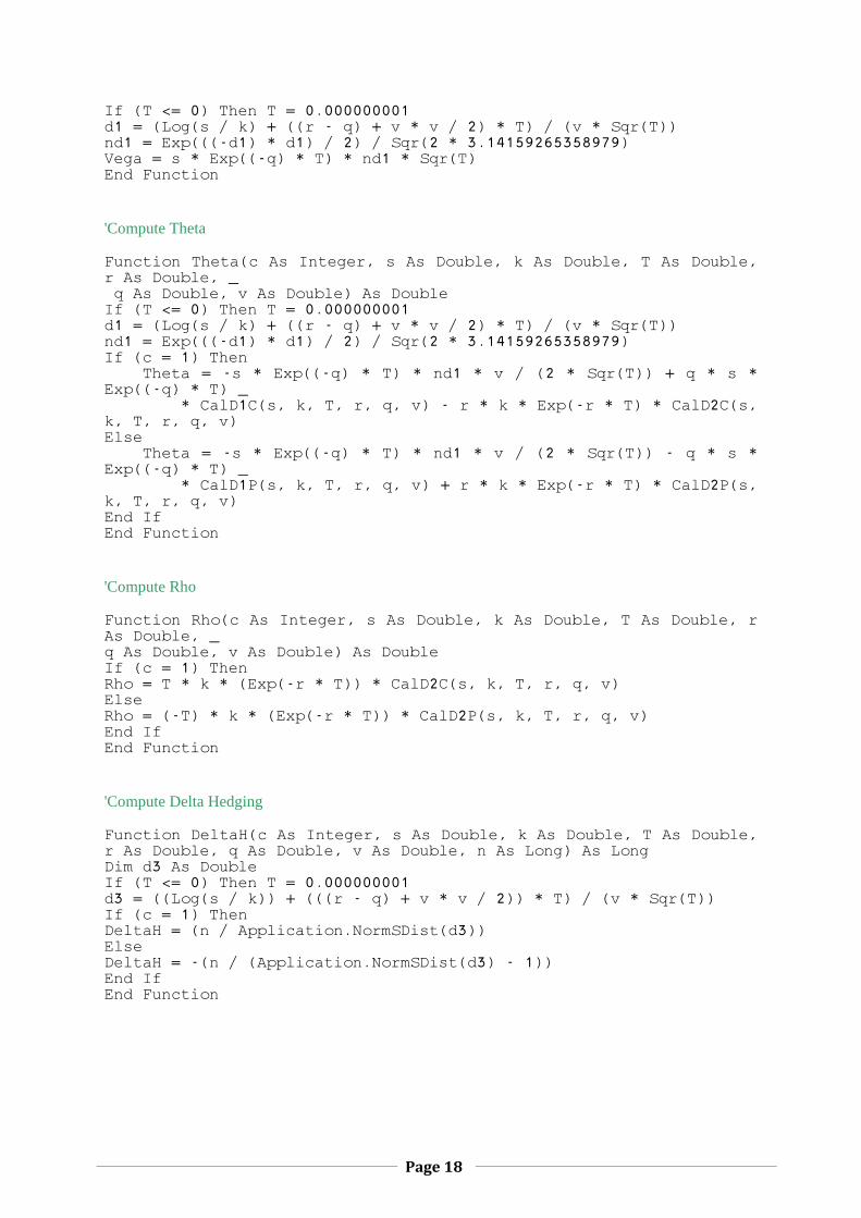
If (T <= 0) Then T = 0.000000001 d1 = (Log(s / k) + ((r - q) + v * v / 2) * T) / (v * Sqr(T)) nd1 = Exp(((-d1) * d1) / 2) / Sqr(2 * 3.14159265358979) Vega = s * Exp((-q) * T) * nd1 * Sqr(T) End Function

'Compute Theta

Function Theta(c As Integer, s As Double, k As Double, T As Double, r As Double, _ q As Double, v As Double) As Double If (T <= 0) Then T = 0.000000001 d1 = (Log(s / k) + ((r - q) + v * v / 2) * T) / (v * Sqr(T)) nd1 = Exp(((-d1) * d1) / 2) / Sqr(2 * 3.14159265358979) If (c = 1) Then Theta = -s * Exp((-q) * T) * nd1 * v / (2 * Sqr(T)) + q * s * Exp((-q) * T) _ * CalD1C(s, k, T, r, q, v) - r * k * Exp(-r * T) * CalD2C(s, k, T, r, q, v) Else Theta = -s * Exp((-q) * T) * nd1 * v / (2 * Sqr(T)) - q * s * Exp((-q) * T) _ * CalD1P(s, k, T, r, q, v) + r * k * Exp(-r * T) * CalD2P(s, k, T, r, q, v) End If End Function

'Compute Rho

Function Rho(c As Integer, s As Double, k As Double, T As Double, r As Double, _ q As Double, v As Double) As Double If (c = 1) Then Rho = T * k * (Exp(-r * T)) * CalD2C(s, k, T, r, q, v) Else Rho = (-T) * k * (Exp(-r * T)) * CalD2P(s, k, T, r, q, v) End If End Function

'Compute Delta Hedging

Function DeltaH(c As Integer, s As Double, k As Double, T As Double, r As Double, q As Double, v As Double, n As Long) As Long Dim d3 As Double If (T <= 0) Then T = 0.000000001 d3 = ((Log(s / k)) + (((r - q) + v * v / 2)) * T) / (v * Sqr(T)) If (c = 1) Then DeltaH = (n / Application.NormSDist(d3)) Else DeltaH = -(n / (Application.NormSDist(d3) - 1)) End If End Function

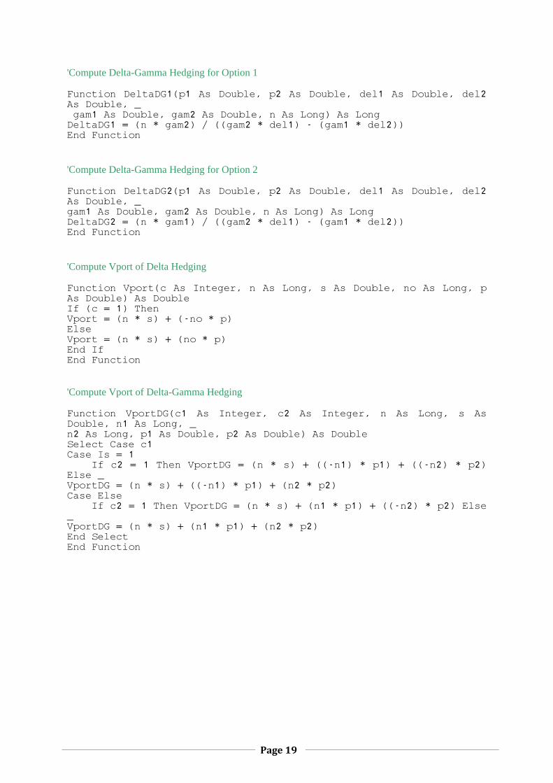
'Compute Delta-Gamma Hedging for Option 1

Function DeltaDG1(p1 As Double, p2 As Double, del1 As Double, del2 As Double, _ gam1 As Double, gam2 As Double, n As Long) As Long DeltaDG1 = (n * gam2) / ((gam2 * del1) - (gam1 * del2)) End Function

'Compute Delta-Gamma Hedging for Option 2

Function DeltaDG2(p1 As Double, p2 As Double, del1 As Double, del2 As Double, _ gam1 As Double, gam2 As Double, n As Long) As Long DeltaDG2 = (n * gam1) / ((gam2 * del1) - (gam1 * del2)) End Function

'Compute Vport of Delta Hedging

Function Vport(c As Integer, n As Long, s As Double, no As Long, p As Double) As Double If (c = 1) Then Vport = (n * s) + (-no * p) Else Vport = (n * s) + (no * p) End If End Function 'Compute Vport of Delta-Gamma Hedging

Function VportDG(c1 As Integer, c2 As Integer, n As Long, s As Double, n1 As Long, _ n2 As Long, p1 As Double, p2 As Double) As Double Select Case c1 Case Is = 1 If c2 = 1 Then VportDG = (n * s) + ((-n1) * p1) + ((-n2) * p2) Else _ VportDG = (n * s) + ((-n1) * p1) + (n2 * p2) Case Else If c2 = 1 Then VportDG = (n * s) + (n1 * p1) + ((-n2) * p2) Else _ VportDG = (n * s) + (n1 * p1) + (n2 * p2) End Select End Function

BIBLIOGRAPHY

Hull, C. John, 2006, Options, Futures, and Other Derivatives, 6th Edition, Pearson Education, New Jersey

Ross, S., Westerfield, R., Jaffe, J., 2005, Corporate Finance, 7th Edition, McGraw-Hill/Irwin, New York

Angstman and G. Geoffrey Alaishuski, The “Greeks”, http://rmtf.soa.org/greeks.pdf, 9 May 2002

‘Extending the Black Scholes formula ‘http://finance.bi.no/~bernt/gcc_prog/recipes/recipes/node9.html, 16/05/08.

(http://www.answers.com/topic/hedging, 29/09/08)

Hedging with Options - Jan Römanjanroman.dhis.org/stud/I2008/Hedging/Hedging.pdf · Gamma (Γ)...

Documents

Transcript of Hedging with Options - Jan Römanjanroman.dhis.org/stud/I2008/Hedging/Hedging.pdf · Gamma (Γ)...