Hartree-Fock Theoryteaching:...Hartree-Fock Theory Alston J. Misquitta Centre for Condensed Matter...

Hartree-Fock Theory

Alston J. Misquitta

Centre for Condensed Matter and Materials PhysicsQueen Mary, University of London

February 18, 2020

Intr Matrix Elements HF Funcs Derivation of HF equations

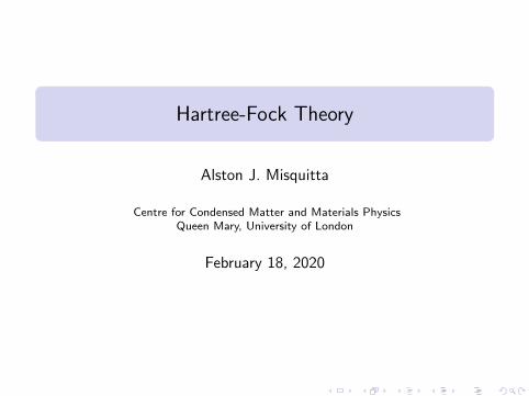
HF in brief I

For an N-electron Slater determinant wavefunction:

Ψ(x1, x2, · · · , xN) =1√N!

∣∣∣∣∣∣∣∣∣χi (x1) χj(x1) · · · χk(x1)χi (x2) χj(x2) · · · χk(x2)

......

. . ....

χi (xN) χj(xN) · · · χk(xN)

∣∣∣∣∣∣∣∣∣≡ |χiχj · · ·χk〉

we will show that the energy is written as:

〈Ψ|H|Ψ〉 =∑i

〈i |h|i〉+∑i>j

[〈ij |ij〉 − 〈ij |ji〉]


HF in brief II

The Hartree–Fock approximation to the ground state energy isfound by varying the spin-orbitals {χi} to minimize the energy:

E0 ≤ EHF = min〈Ψ|H|Ψ〉

subject to the conditions that the spin-orbitals are orthonormal.As before, but with many more steps, the variational principleleads to the following equations for the spin-orbitals

f (i)χ(xi ) = εχ(xi )

where f (i) is an effective operator called the Fock operator

f (i) = −1

2∇2

i −∑α

Zαriα

+ vHF(i)


HF in brief III

where vHF(i) is the Hartree–Fock effective potential that dependson the solutions to the above equations. So we must solve theseequations self-consistently: Make a guess for the solutions;construct the potential vHF(i) from this guess; solve the Fockequations; get new solutions; and repeat till convergence.


Matrix Elements I

We will require a number of matrix elements for Hartree–Fock andpost-HF methods. You have already seen these when we workedthrough the H2 system. The rules for general N-electron matrixelements are very similar to those for the 2-electron case; the onlycomplication is the added complication brought out by the algebriccomplexity of the N-electron Slater determinants.

Szabo & Ostlund describes the calculation of these matrixelements in some detail and I expect you to look through thosederivations in case the ones presented here are not clear enough foryou. A problem with the S&O derivations is that they are too long.More on this soon.


Matrix Elements II

We are after matrix elements of the form

〈K |O1|L〉 and 〈K |O2|L〉

where |K/L〉 are N-electron Slater determinant wavefunctions. Ingeneral, the N-electron determinant |Ψ〉 can be written as

|Ψ〉 =1√N!

N!∑u=1

σuPu{χ1(1)χ2(2) · · ·χN(N)}

Here Pu is a permutation operator that can be expressed as aproduct of binary permutations:

Pu = PijPkl · · ·

and σu is phase factor that is +1 if Pu contains an even number ofbinary permutations and is −1 otherwise.


Matrix Elements III

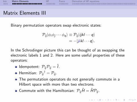
Binary permutation operators swap electronic states:

Pij |φiφj · · ·φq〉 ≡ Pij |ijkl · · · q〉= −|jikl · · · q〉.

In the Schrodinger picture this can be thought of as swapping theelectronic labels 1 and 2. Here are some useful properties of theseoperators:

Idempotent: PijPij = I .

Hermitian: Pij † = Pij .The permutation operators do not generally commute in aHilbert space with more than two electrons.

Commute with the Hamiltonian: Pij H = HPij .


Matrix Elements IV

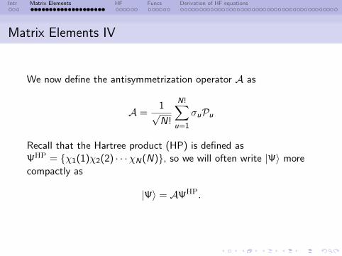
We now define the antisymmetrization operator A as

A =1√N!

N!∑u=1

σuPu

Recall that the Hartree product (HP) is defined asΨHP = {χ1(1)χ2(2) · · ·χN(N)}, so we will often write |Ψ〉 morecompactly as

|Ψ〉 = AΨHP.


Matrix Elements V

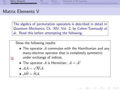
The algebra of permutation operators is described in detail inQuantum Mechanics, Ch. XIV, Vol. 2, by Cohen-Tannoudji etal.. Read this before attempting the following.

Q:

Show the following results:

The operator A commutes with the Hamiltonian and anymany-electron operator that is completely symmetricunder exchange of indices.

The operator A is Hermitian: A = A†

AA =√

N!A.

AH = HA.


Matrix Elements VI

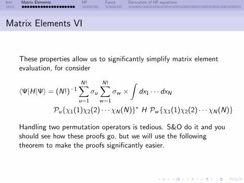
These properties allow us to significantly simplify matrix elementevaluation, for consider

〈Ψ|H|Ψ〉 = (N!)−1N!∑u=1

σu

N!∑w=1

σw ×∫

dx1 · · · dxN

Pu{χ1(1)χ2(2) · · ·χN(N)}∗ H Pw{χ1(1)χ2(2) · · ·χN(N)}

Handling two permutation operators is tedious. S&O do it and youshould see how these proofs go, but we will use the followingtheorem to make the proofs significantly easier.


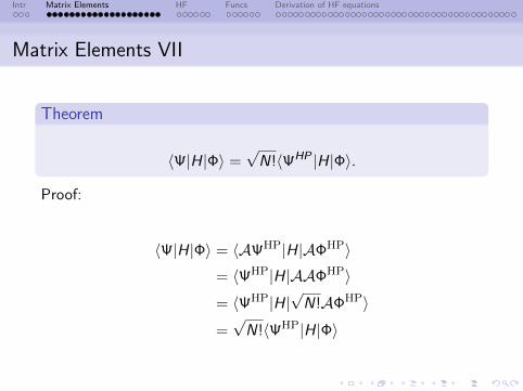
Matrix Elements VII

Theorem

〈Ψ|H|Φ〉 =√

N!〈ΨHP |H|Φ〉.

Proof:

〈Ψ|H|Φ〉 = 〈AΨHP|H|AΦHP〉= 〈ΨHP|H|AAΦHP〉

= 〈ΨHP|H|√

N!AΦHP〉

=√

N!〈ΨHP|H|Φ〉


Matrix Elements VIII

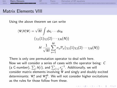
Using the above theorem we can write

〈Ψ|H|Ψ〉 =√

N!

∫dx1 · · · dxN

{χ1(1)χ2(2) · · ·χN(N)}

H1√N!

N!∑u=1

σuPu{χ1(1)χ2(2) · · ·χN(N)}

There is only one permutation operator to deal with here.Now we will consider a series of cases with the operator being: C(a C-number),

∑i h(i), and

∑i>j r−1ij . Additionally, we will

consider matrix elements involving Ψ and singly and doubly exciteddeterminants: Ψa

i and Ψabij . We will not consider higher excitations

as the rules for those follow from these.


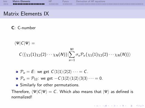
Matrix Elements IX

C: C-number

〈Ψ|C |Ψ〉 =

C 〈{χ1(1)χ2(2) · · ·χN(N)}|N!∑u=1

σuPu{χ1(1)χ2(2) · · ·χN(N)}〉

Pu = E : we get C 〈1|1〉〈2|2〉 · · · = C .

Pu = P12: we get −C 〈1|2〉〈1|2〉〈3|3〉 · · · = 0.

Similarly for other permutations.

Therefore, 〈Ψ|C |Ψ〉 = C . Which also means that |Ψ〉 as defined isnormalized!


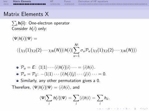
Matrix Elements X∑i h(i): One-electron operator

Consider h(i) only:

〈Ψ|h(i)|Ψ〉 =

〈{χ1(1)χ2(2) · · ·χN(N)}|h(i)|N!∑u=1

σuPu{χ1(1)χ2(2) · · ·χN(N)}〉

Pu = E : 〈1|1〉 · · · 〈i |h(i)|i〉 · · · = 〈i |h|i〉.Pu = Pij : −〈1|1〉 · · · 〈i |h(i)|j〉 · · · 〈j |i〉 · · · = 0.

Similarly, any other permutation gives a 0.

Therefore, 〈Ψ|h(i)|Ψ〉 = 〈i |h|i〉, and

〈Ψ|∑i

h(i)|Ψ〉 =∑i

〈i |h|i〉 =∑i

hii .


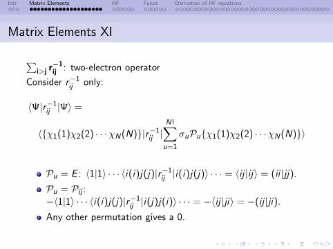
Matrix Elements XI

∑i>j r

−1ij : two-electron operator

Consider r−1ij only:

〈Ψ|r−1ij |Ψ〉 =

〈{χ1(1)χ2(2) · · ·χN(N)}|r−1ij |N!∑u=1

σuPu{χ1(1)χ2(2) · · ·χN(N)}〉

Pu = E : 〈1|1〉 · · · 〈i(i)j(j)|r−1ij |i(i)j(j)〉 · · · = 〈ij |ij〉 = (ii |jj).

Pu = Pij :−〈1|1〉 · · · 〈i(i)j(j)|r−1ij |i(j)j(i)〉 · · · = −〈ij |ji〉 = −(ij |ji).

Any other permutation gives a 0.


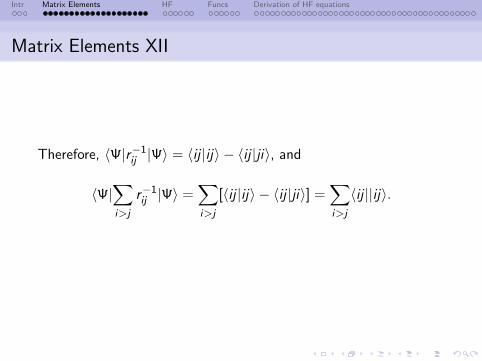
Matrix Elements XII

Therefore, 〈Ψ|r−1ij |Ψ〉 = 〈ij |ij〉 − 〈ij |ji〉, and

〈Ψ|∑i>j

r−1ij |Ψ〉 =∑i>j

[〈ij |ij〉 − 〈ij |ji〉] =∑i>j

〈ij ||ij〉.


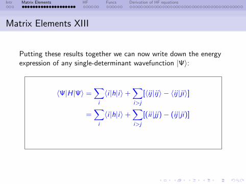
Matrix Elements XIII

Putting these results together we can now write down the energyexpression of any single-determinant wavefunction |Ψ〉:

〈Ψ|H|Ψ〉 =∑i

〈i |h|i〉+∑i>j

[〈ij |ij〉 − 〈ij |ji〉]

=∑i

〈i |h|i〉+∑i>j

[(ii |jj)− (ij |ji)]


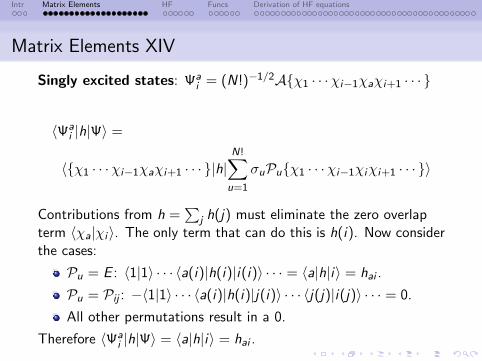
Matrix Elements XIV

Singly excited states: Ψai = (N!)−1/2A{χ1 · · ·χi−1χaχi+1 · · · }

〈Ψai |h|Ψ〉 =

〈{χ1 · · ·χi−1χaχi+1 · · · }|h|N!∑u=1

σuPu{χ1 · · ·χi−1χiχi+1 · · · }〉

Contributions from h =∑

j h(j) must eliminate the zero overlapterm 〈χa|χi 〉. The only term that can do this is h(i). Now considerthe cases:

Pu = E : 〈1|1〉 · · · 〈a(i)|h(i)|i(i)〉 · · · = 〈a|h|i〉 = hai .

Pu = Pij : −〈1|1〉 · · · 〈a(i)|h(i)|j(i)〉 · · · 〈j(j)|i(j)〉 · · · = 0.

All other permutations result in a 0.

Therefore 〈Ψai |h|Ψ〉 = 〈a|h|i〉 = hai .


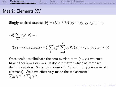
Matrix Elements XV

Singly excited states: Ψai = (N!)−1/2A{χ1 · · ·χi−1χaχi+1 · · · }

〈Ψai |∑kl

r−1kl |Ψ〉 =

〈{χ1 · · ·χi−1χaχi+1 · · · }|∑kl

r−1kl |N!∑u=1

σuPu{χ1 · · ·χi−1χiχi+1 · · · }〉

Once again, to eliminate the zero overlap term 〈χa|χi 〉 we musthave either k = i or l = i . It doesn’t matter which as these aredummy variables. So let us choose k = i and l = j (j goes over allelectrons). We have effectively made the replacement:∑

kl r−1kl →∑

j r−1ij .


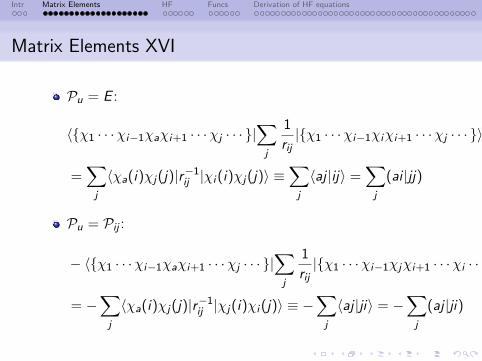
Matrix Elements XVI

Pu = E :

〈{χ1 · · ·χi−1χaχi+1 · · ·χj · · · }|∑j

1

rij|{χ1 · · ·χi−1χiχi+1 · · ·χj · · · }〉

=∑j

〈χa(i)χj(j)|r−1ij |χi (i)χj(j)〉 ≡∑j

〈aj |ij〉 =∑j

(ai |jj)

Pu = Pij :

− 〈{χ1 · · ·χi−1χaχi+1 · · ·χj · · · }|∑j

1

rij|{χ1 · · ·χi−1χjχi+1 · · ·χi · · · }〉

= −∑j

〈χa(i)χj(j)|r−1ij |χj(i)χi (j)〉 ≡ −∑j

〈aj |ji〉 = −∑j

(aj |ji)


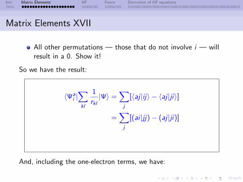
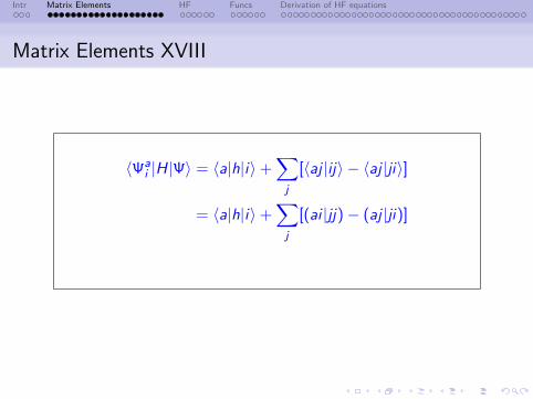
Matrix Elements XVIII

〈Ψai |H|Ψ〉 = 〈a|h|i〉+

∑j

[〈aj |ij〉 − 〈aj |ji〉]

= 〈a|h|i〉+∑j

[(ai |jj)− (aj |ji)]


Matrix Elements XIX

Doubly excited states:Ψab

ij = (N!)−1/2A{χ1 · · ·χi−1χaχi+1 · · ·χj−1χbχj+1 · · · }

Q:

Show that

There are no contributions from the one-electronoperator h =

∑i h(i).

The two-electron operator∑

kl1rkl

results in singlecontribution: (ai |bj)− (aj |bi). No summations here.

Consequently,

〈Ψabij |∑kl

1

rkl|Ψ〉 = 〈ab|ij〉 − 〈ab|ji〉 = (ai |bj)− (aj |bi)


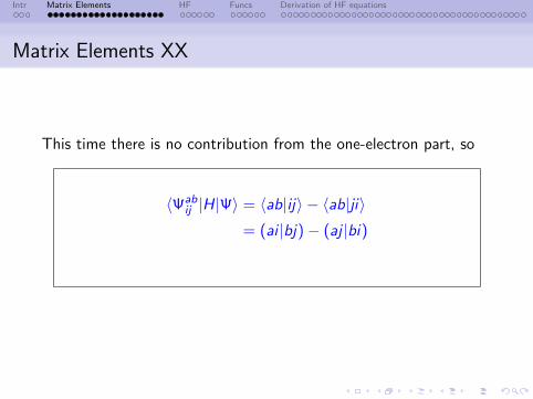
Matrix Elements XX

This time there is no contribution from the one-electron part, so

〈Ψabij |H|Ψ〉 = 〈ab|ij〉 − 〈ab|ji〉

= (ai |bj)− (aj |bi)


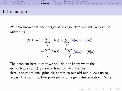
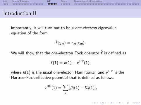
Introduction II

importantly, it will turn out to be a one-electron eigenvalueequation of the form

f |χm〉 = εm|χm〉.

We will show that the one-electron Fock operator f is defined as

f (1) = h(1) + vHF(1),

where h(1) is the usual one-electon Hamiltonian and vHF is theHartree–Fock effective potential that is defined as follows:

vHF(1) =∑i

[Ji (1)−Ki (1)],


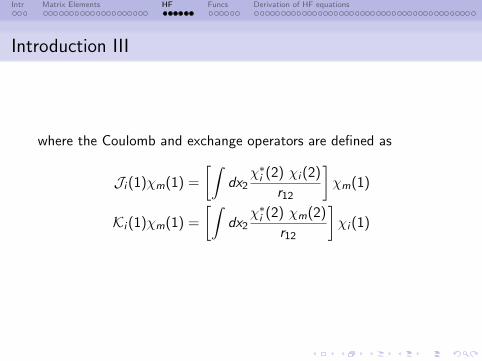
Introduction III

where the Coulomb and exchange operators are defined as

Ji (1)χm(1) =

[∫dx2

χ∗i (2) χi (2)

r12

]χm(1)

Ki (1)χm(1) =

[∫dx2

χ∗i (2) χm(2)

r12

]χi (1)


Introduction IV

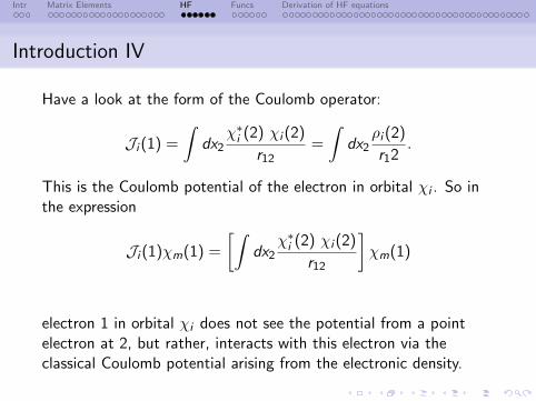
Have a look at the form of the Coulomb operator:

Ji (1) =

∫dx2

χ∗i (2) χi (2)

r12=

∫dx2

ρi (2)

r12.

This is the Coulomb potential of the electron in orbital χi . So inthe expression

Ji (1)χm(1) =

[∫dx2

χ∗i (2) χi (2)

r12

]χm(1)

electron 1 in orbital χi does not see the potential from a pointelectron at 2, but rather, interacts with this electron via theclassical Coulomb potential arising from the electronic density.


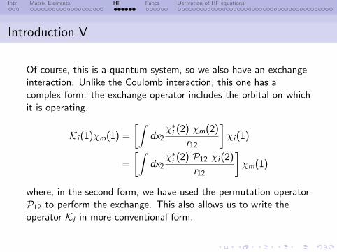
Introduction V

Of course, this is a quantum system, so we also have an exchangeinteraction. Unlike the Coulomb interaction, this one has acomplex form: the exchange operator includes the orbital on whichit is operating.

Ki (1)χm(1) =

[∫dx2

χ∗i (2) χm(2)

r12

]χi (1)

=

[∫dx2

χ∗i (2) P12 χi (2)

r12

]χm(1)

where, in the second form, we have used the permutation operatorP12 to perform the exchange. This also allows us to write theoperator Ki in more conventional form.


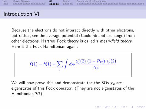
Introduction VI

Because the electrons do not interact directly with other electrons,but rather, see the average potential (Coulomb and exchange) fromother electrons, Hartree–Fock theory is called a mean-field theory.Here is the Fock Hamiltonian again:

f (1) = h(1) +∑i

∫dx2

χ∗i (2) (1− P12) χi (2)

r12

We will now prove this and demonstrate the the SOs χa areeigenstates of this Fock operator. (They are not eigenstates of theHamiltonian H!)


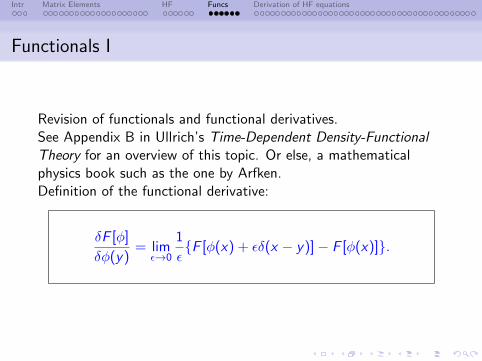
Functionals I

Revision of functionals and functional derivatives.See Appendix B in Ullrich’s Time-Dependent Density-FunctionalTheory for an overview of this topic. Or else, a mathematicalphysics book such as the one by Arfken.Definition of the functional derivative:

δF [φ]

δφ(y)= lim

ε→0

1

ε{F [φ(x) + εδ(x − y)]− F [φ(x)]}.


Functionals II

Alternative definition:If F [y ] is a functional of y(x), and if δy(x) is some arbitraryvariation in y , then we may define dF = F [y + δy ]− F [y ]. Thefunctional derivative of F [y ] w.r.t. y(x) is then defined via

dF =

∫dxδF [y ]

δy(x)δy(x).

The latter definition is often more useful than the first, though thefirst is the one we should fall back on in case of doubt.


Functionals III

Q:

F [y ] =

∫y(x)2dx .

Show that

δF [y ]

δy(x)= 2y(x).

Use both definitions to do this.


Functionals IV

Useful results:

F [φ] = g(φ(x))

δF [φ]

δφ(y)=δg(φ(x))

δφ(y)= g ′(φ(x))δ(x − y).

F [φ] =∫

g(φ(x))dx

δF [φ]

δφ(y)= g ′(φ(y)).

F [φ] =∫

g(∇φ(x))dx

δF [φ]

δφ(y)= −∇g ′(∇φ(y)).

The last result follows using integration by parts. Using the aboveyou can derive the Euler–Lagrange equations for the functionalF [x , y(x), y ′(x)]. Try it.


Functionals V

Product Rule:

δF [φ]G [φ]

δφ(y)= F [φ]

δG [φ]

δφ(y)+δF [φ]

δφ(y)G [φ].

Chain Rule:

δF [γ[φ]]

δφ(y)=

∫dy ′

δF [γ]

δγ(y ′)

δγ(y ′)

δφ(y).


Functionals VI

When we write the energy in terms of the spin-orbitals we will endup with expressions that involve both χi and its complex conjugateχ∗i . Mathematically these are independent functions. One way oflooking at this is to consider that the real and imaginary parts ofthe spin-orbitals can be varied independently.A consequence of this is that the energy functional can be thoughtof as being a functional of both χi and χ∗i . So the variation can becarried out w.r.t. either, or both. But as the Hamiltonian isHermitian, only one need be considered, and it is usually moreconvenient to conduct the variation w.r.t. χ∗i .


HF: Derivation I

We need to minimize:

E0[{χi}] = 〈Ψ|H|Ψ〉 =∑i

〈i |h|i〉+1

2

∑i ,j

[〈ij |ij〉 − 〈ij |ji〉]

w.r.t. the {χi} subject to the conditions 〈χi |χj〉 = δij . Theorthonormality condition can be included using the method ofLagrange multipliers, i.e., we minimize the functional

L[{χi}] = E0[{χi}]−N∑ij

εji (〈χi |χj〉 − δij)


HF: Derivation II

First a result we will need:

Q:

We will impose the condition that L is real. This is reasonableas the energy is real. Show that this condition implies εji = ε∗ij ,i.e., the Lagrange multiplier matrix is Hermitian.

Hint: Set sij = 〈χi |χj〉−δij and consider the real sum∑

ij εji sij .Use the fact that sij = s∗ji to show the required result.


HF: Derivation III

L[{χi}] =∑i

〈i |h|i〉+1

2

∑i ,j

[〈ij |ij〉 − 〈ij |ji〉]−N∑ij

εji (〈χi |χj〉 − δij)

0 =δLδ〈k |

= h|k〉+1

2

∑j

〈j | 1

r12|j〉|k〉+

1

2

∑i

〈i | 1

r12|i〉|k〉

− 1

2

∑j

〈j | 1

r12|k〉|j〉 − 1

2

∑i

〈i | 1

r12|k〉|i〉 −

∑j

εjk |j〉

= h|k〉+∑i

〈i | 1

r12|i〉|k〉 −

∑i

〈i | 1

r12|k〉|i〉 −

∑i

εik |i〉


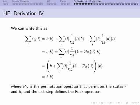
HF: Derivation IV

We can write this as∑i

εik |i〉 = h|k〉+∑i

〈i | 1

r12|i〉|k〉 −

∑i

〈i | 1

r12|k〉|i〉

= h|k〉+∑i

〈i | 1

r12(1− Pik)|i〉|k〉

=

(h +

∑i

〈i | 1

r12(1− Pik)|i〉

)|k〉

= f |k〉

where Pik is the permutation operator that permutes the states iand k , and the last step defines the Fock operator.


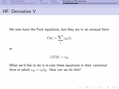
HF: Derivation V

We now have the Fock equations, but they are in an unusual form:

f |k〉 =∑i

εik |i〉,

or

〈i |f |k〉 = εik .

What we’d like to do is re-cast these equations in their canonicalform in which εik = εkδik . How can we do this?


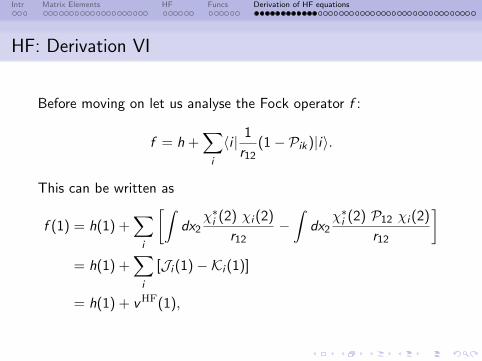
HF: Derivation VI

Before moving on let us analyse the Fock operator f :

f = h +∑i

〈i | 1

r12(1− Pik)|i〉.

This can be written as

f (1) = h(1) +∑i

[∫dx2

χ∗i (2) χi (2)

r12−∫

dx2χ∗i (2) P12 χi (2)

r12

]= h(1) +

∑i

[Ji (1)−Ki (1)]

= h(1) + vHF(1),


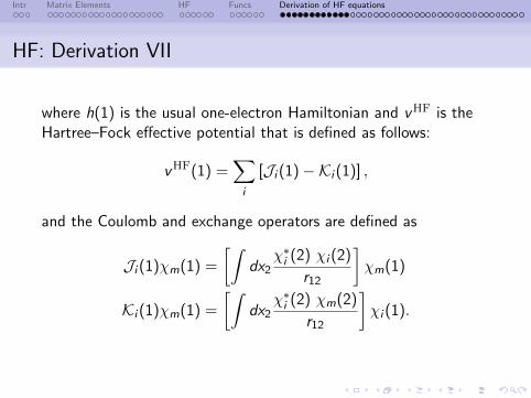
HF: Derivation VII

where h(1) is the usual one-electron Hamiltonian and vHF is theHartree–Fock effective potential that is defined as follows:

vHF(1) =∑i

[Ji (1)−Ki (1)] ,

and the Coulomb and exchange operators are defined as

Ji (1)χm(1) =

[∫dx2

χ∗i (2) χi (2)

r12

]χm(1)

Ki (1)χm(1) =

[∫dx2

χ∗i (2) χm(2)

r12

]χi (1).


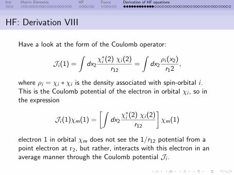
HF: Derivation VIII

Have a look at the form of the Coulomb operator:

Ji (1) =

∫dx2

χ∗i (2) χi (2)

r12=

∫dx2

ρi (x2)

r12,

where ρi = χi ∗ χi is the density associated with spin-orbital i .This is the Coulomb potential of the electron in orbital χi , so inthe expression

Ji (1)χm(1) =

[∫dx2

χ∗i (2) χi (2)

r12

]χm(1)

electron 1 in orbital χm does not see the 1/r12 potential from apoint electron at r2, but rather, interacts with this electron in anaverage manner through the Coulomb potential Ji .


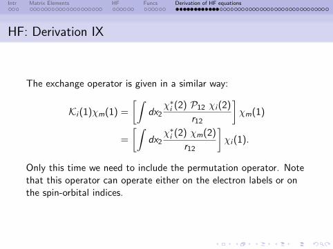
HF: Derivation IX

The exchange operator is given in a similar way:

Ki (1)χm(1) =

[∫dx2

χ∗i (2) P12 χi (2)

r12

]χm(1)

=

[∫dx2

χ∗i (2) χm(2)

r12

]χi (1).

Only this time we need to include the permutation operator. Notethat this operator can operate either on the electron labels or onthe spin-orbital indices.


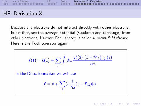
HF: Derivation X

Because the electrons do not interact directly with other electrons,but rather, see the average potential (Coulomb and exchange) fromother electrons, Hartree–Fock theory is called a mean-field theory.Here is the Fock operator again:

f (1) = h(1) +∑i

∫dx2

χ∗i (2) (1− P12) χi (2)

r12

In the Dirac formalism we will use

f = h +∑i

〈i | 1

r12(1− Pik)|i〉.


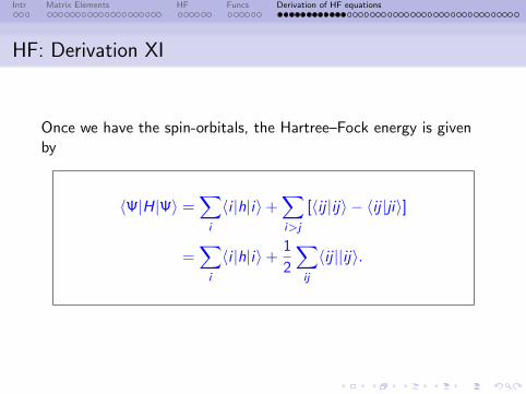
HF: Derivation XI

Once we have the spin-orbitals, the Hartree–Fock energy is givenby

〈Ψ|H|Ψ〉 =∑i

〈i |h|i〉+∑i>j

[〈ij |ij〉 − 〈ij |ji〉]

=∑i

〈i |h|i〉+1

2

∑ij

〈ij ||ij〉.


HF: Derivation XII

Q:What does the sum over i go over in the Fock operator? Allspin-orbitals? Only some sub-set of them?

Q:In the Dirac notation we have the permutation operator Pik .What is k here?

Q:In what sense is the permutation operator Pik that acts on spin-orbital labels equivalent to the operator P12 that exchangeselectron labels?

Q:How many solutions to the Fock equation are there? I.e., whatis the dimension of the energy matrix ε?


Canonical form I

The Fock equations in their non-canonical form are given by

f |i〉 =∑i

εji |j〉.

This implies that we can define the energy matrix:

εij =〈i |f |j〉.

We have shown that ε is an Hermitian matrix, so we can alwaysfind a Unitary matrix, U that diagonalises it giving the diagonalmatrix ε′. That is

ε′ = U†εU,


Canonical form III

In this basis of what are called the canonical orbitals, the energymatrix is diagonal so the Fock equations become

f |i ′〉 =∑i

ε′ji |j ′〉

=∑i

ε′iδij |j ′〉

= ε′i |i ′〉.

Equivalently we can write this as

f χ′i = ε′iχ′i .

This is the usual form of an eigenvalue equation. When codes likeNWChem present the spin-orbitals they present them in this,canonical, form.


Canonical form IV

There is one complication with the previous derivation: the Fockoperator is defined in terms of the spin orbitals {χi}, so when wetransform to the canonical orbitals {χ′i} we will have also changed

f to f ′. This would seem to imply that we have made afundamental change to the problem we were trying to solve.However, as we will now show, the form of the Fock operatorimplies that it remains invariant under a unitary transformation.

f (1) = h(1) +∑i

∫dx2

χ∗i (2) (1− P12) χi (2)

r12

The one-electron Hamiltonian h(1) does not depend on thespin-orbitals so the unitary transformation has no effect on thisterm.


Canonical form V

Consider the Coulomb operator:∑i

J ′i (1) =∑i

∫dx2

χ′i∗(2) χ′i (2)

r12

=∑kl

∑i

[U∗kiUli ]

∫dx2

χ∗k(2) χl(2)

r12

=∑kl

[δkl ]

∫dx2

χ∗k(2) χl(2)

r12

=∑k

∫dx2

χ∗k(2) χk(2)

r12

=∑i

Ji (2) change of dummy index.

Here, the indices i , k , l all go over occupied orbitals only.


Canonical form VI

Q:

Show that the exchange operator is also unchanged under aunitary transformation of the occupied orbitals. I.e. show that∑

i K′i =∑

i Ki .

Hence we get our result: f ′(1) = f (1): the Fock operator isinvariant under a unitary transformation of the occupiedspin-orbitals. Henceforth we always deal with canonicalspin-orbitals and drop the primes to write:

f χi = εiχi .


Canonical form VII

Pause here: Why does the unitary transformation apply to theoccupied spin-orbitals only? Better yet, what do we mean byoccupied?

The Fock operator yields an infinite number of solutions.

The ground-state is usually obtained by placing theelectron in the lowest energy spin-orbitals. These will bethe occupied orbitals.

The remaining will be the un-occupied or virtual orbitals.

The Fock operator itself contains only the occupiedorbitals.

Q: What is meant by the last statement?


Canonical form VIII

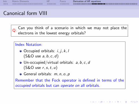
Q:Can you think of a scenario in which we may not place theelectrons in the lowest energy orbitals?

Index Notation:

Occupied orbitals: i , j , k , l(S&O use a, b, c , d)

Un-occupied/virtual orbitals: a, b, c , d(S&O use r , s, t, u)

General orbitals: m, n, o, p

Remember that the Fock operator is defined in terms of theoccupied orbitals but can operate on all orbitals.


Canonical form IX

Notes:

The canonical spin orbitals are generally delocalised.

Like the non-canonical SOs, they are orthonormal.

We have proved that we can obtain a set of canonical SOs forthe occupied orbitals. It turns out that this can be done forthe virtual (un-occupied) SOs too.


Orbital Energies I

What do the spin orbitals and orbitals energies mean? When wesolve the Fock equations we formally obtain an infinity of solutions(any partial differential equation has an infinity of solutions). Weplace the N electrons in the N lowest energy SOs. These are ouroccupied orbitals. The others, the un-occupied ones, are called thevirtual SOs. There are an infinity of these (formally!). We will nowtry to understand what these orbitals mean. But first, somethingto think about

Q:

Why have we assumed (as we will) that the putting the elec-trons in the N lowest energy SOs is the correct thing to do?After all, our goal is to minimize the energy E0 which, as wewill soon see, is not the same as the sum of the energies of theoccupied SOs.


Orbital Energies II

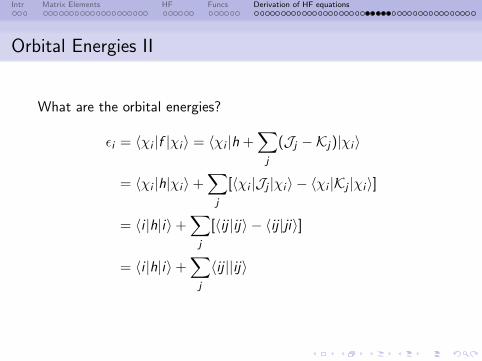
What are the orbital energies?

εi = 〈χi |f |χi 〉 = 〈χi |h +∑j

(Jj −Kj)|χi 〉

= 〈χi |h|χi 〉+∑j

[〈χi |Jj |χi 〉 − 〈χi |Kj |χi 〉]

= 〈i |h|i〉+∑j

[〈ij |ij〉 − 〈ij |ji〉]

= 〈i |h|i〉+∑j

〈ij ||ij〉


Orbital Energies III

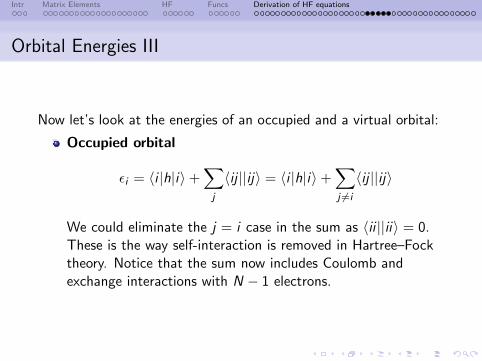
Now let’s look at the energies of an occupied and a virtual orbital:

Occupied orbital

εi = 〈i |h|i〉+∑j

〈ij ||ij〉 = 〈i |h|i〉+∑j 6=i

〈ij ||ij〉

We could eliminate the j = i case in the sum as 〈ii ||ii〉 = 0.These is the way self-interaction is removed in Hartree–Focktheory. Notice that the sum now includes Coulomb andexchange interactions with N − 1 electrons.


Orbital Energies IV

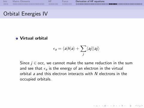
Virtual orbital

εa = 〈a|h|a〉+∑j

〈aj ||aj〉

Since j ∈ occ, we cannot make the same reduction in the sumand see that εa is the energy of an electron in the virtualorbital a and this electron interacts with N electrons in theoccupied orbitals.


Orbital Energies V

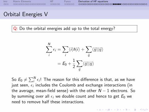
Q: Do the orbital energies add up to the total energy?

N∑i

εi =∑i

〈i |h|i〉+∑ij

〈ij ||ij〉

= E0 +1

2

∑ij

〈ij ||ij〉

So E0 6=∑N

i εi ! The reason for this difference is that, as we havejust seen, εi includes the Coulomb and exchange interactions (inthe average, mean-field sense) with the other N − 1 electrons. Soby summing over all εi we double count and hence to get E0 weneed to remove half these interactions.


Koopman’s Theorem I

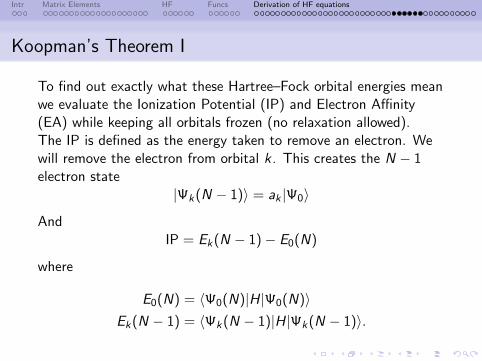
To find out exactly what these Hartree–Fock orbital energies meanwe evaluate the Ionization Potential (IP) and Electron Affinity(EA) while keeping all orbitals frozen (no relaxation allowed).The IP is defined as the energy taken to remove an electron. Wewill remove the electron from orbital k . This creates the N − 1electron state

|Ψk(N − 1)〉 = ak |Ψ0〉

AndIP = Ek(N − 1)− E0(N)

where

E0(N) = 〈Ψ0(N)|H|Ψ0(N)〉Ek(N − 1) = 〈Ψk(N − 1)|H|Ψk(N − 1)〉.


Koopman’s Theorem II

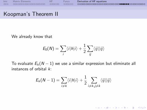
We already know that

E0(N) =∑i

〈i |h|i〉+1

2

∑ij

〈ij ||ij〉

To evaluate Ek(N − 1) we use a similar expression but eliminate allinstances of orbital k:

Ek(N − 1) =∑i 6=k

〈i |h|i〉+1

2

∑i 6=k,j 6=k

〈ij ||ij〉


Koopman’s Theorem III

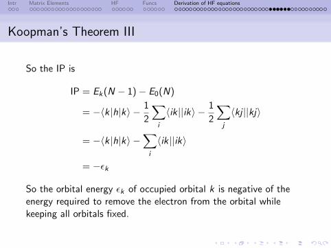
So the IP is

IP = Ek(N − 1)− E0(N)

= −〈k |h|k〉 − 1

2

∑i

〈ik ||ik〉 − 1

2

∑j

〈kj ||kj〉

= −〈k |h|k〉 −∑i

〈ik ||ik〉

= −εk

So the orbital energy εk of occupied orbital k is negative of theenergy required to remove the electron from the orbital whilekeeping all orbitals fixed.


Koopman’s Theorem IV

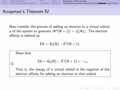
Now consider the process of adding an electron to a virtual orbitala of the system to generate |Ψa(N + 1)〉 = a†a|Ψ0〉. The electronaffinity is defined as

EA = E0(N)− E a(N + 1).

Q:

Show that

EA = E0(N)− E a(N + 1) = −εa

That is, the energy of a virtual orbital is the negative of theelectron affinity for adding an electron to that orbital.


Koopman’s Theorem V

This now explains why an electron in a virtual orbital has anenergies that is consistent with it interacting with N otherelectrons. From the above we see that this is so because theenergy of a virtual orbital is (minus) the energy required to createan N + 1 state.


Koopman’s Theorem VI

Koopmans’ TheoremGiven an N-electron Hartree–Fock single determinant with oc-cupied and virtual spin orbital energues εi and εa, the ionizationpotential to produce an N − 1-electron state with all orbitalsfrozen and the electron removed from orbital i is −εi , and theelectron affinity to produce a N + 1-electron state with an ad-ditional electron in virtual orbital a is −εa.


Brillioun’s Theorem I

Brillioun’s theorem deals with the stability of the Hartree–Focksolution w.r.t. first-order changes to the wavefunction (the Focksingle-determinant).We have derived the Fock equations using the variational principle,so, the solutions to the Fock equations should be stable in thevariational sense, that is, the Hartree–Fock energy should notchange (to first order) with small changes to the wavefunction.What Brillioun’s Theorem tells us is that this is indeed true if bysmall changes we mean single excitations: that is, singleexcitations will not change the Hartree–Fock energy.


Brillioun’s Theorem II

Brillioun’s theorem states that a singly-excited determinant Ψai

does not connect to the HF solution Ψ0 via the Hamiltonian.I.e.,

〈Ψai |H|Ψ0〉 = 0.

To demonstrate this we need a couple of results:

〈Ψai |H|Ψ0〉 = 〈a|h|i〉+

∑j

[〈aj |ij〉 − 〈aj |ji〉]

= 〈a|h|i〉+∑j

〈aj ||ij〉


Brillioun’s Theorem III

and we need the general form of matrix elements of the Fockoperator:

fmn = 〈χm|f |χn〉 = 〈χm|h +∑j

(Jj −Kj)|χn〉

= 〈χm|h|χn〉+∑j

[〈χm|Jj |χn〉 − 〈χm|Kj |χn〉]

= 〈m|h|n〉+∑j

[〈mj |nj〉 − 〈mj |jn〉]

= 〈m|h|n〉+∑j

〈mj ||nj〉

Since the SOs χm are eigenstates of the Fock operator, we have

fmn = 〈χm|f |χn〉 = εn〈χm|χn〉 = εnδmn.


Brillioun’s Theorem IV

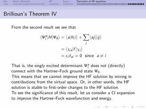
From the second result we see that

〈Ψai |H|Ψ0〉 = 〈a|h|i〉+

∑j

〈aj ||ij〉

= 〈χa|f |χi 〉= εiδai = 0 since a 6= i

That is, the singly excited determinant Ψai does not (directly)

connect with the Hartree–Fock ground state Ψ0.This means that we cannot improve the HF solution by mixing incontributions from the virtual space. Or, in other words, the HFsolution is stable to first-order changes to the HF solution.To see the significance of this result, let us consider a CI expansionto improve the Hartree–Fock wavefunction and energy.


Brillioun’s Theorem V

1

2

n

n + 1

n + m

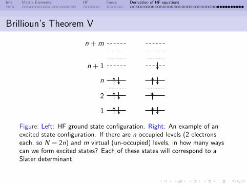
Figure: Left: HF ground state configuration. Right: An example of anexcited state configuration. If there are n occupied levels (2 electronseach, so N = 2n) and m virtual (un-occupied) levels, in how many wayscan we form excited states? Each of these states will correspond to aSlater determinant.


Brillioun’s Theorem VI

We generate the full CI (FCI) wavefunction by including all kindsof single determinants in a linear expansion:

|Ψ〉 = c0|Ψ0〉+∑ia

cai |Ψa

i 〉+∑ij ,ab

cabij |Ψab

ij 〉+ · · ·

= c0|Ψ0〉+ cS |S〉+ cD |D〉+ · · ·

where electrons are excited from the occupied orbitals i , j , k , · · · tothe virtual orbitals a, b, c , · · · .We may think that the simplest way to improve the HF solution|Ψ0〉 is to include the single excitations |S〉. This is a reasonableassumption that proves to be wrong because of Brillouin’stheorem. To see this, consider the simple case where we have only


Brillioun’s Theorem VII

one singly excited determinant |Ψai 〉. So the CI — call it CIS for

configuration interaction with single excitations — expansion is

|Ψ〉 = |Ψ0〉+ cai |Ψa

i 〉

Using the usual variational methods we have discussed before todetermine the coefficients c0 and cab

ij we convert this problem intothe set of linear equations(

〈Ψ0|H|Ψ0〉〈Ψ0|H|Ψai 〉

〈Ψai |H|Ψ0〉〈Ψa

i |H|Ψai 〉

)(c0cai

)= E

(c0cai

)From Brillouin’s theorem 〈Ψa

i |H|Ψ0〉 = 0 and 〈Ψ0|H|Ψ0〉 = E0,therefore we get(

E0 00 〈Ψa

i |H|Ψai 〉

)(c0cai

)= E

(c0cai

)


Brillioun’s Theorem VIII

The ground-state solution is simply E = E0 with c0 = 1 andcai = 0. I.e., the ground-state of the CIS variational expansion is

the Hartree–Fock solution. That is, singly excited determinants(on their own) cannot improve the Hartree–Fock solution. I.e.,Hartree–Fock is stable to perturbations that take the form of singleexcitations.

This does not mean that single excitation can never contribute.They can if we also include double excitations. Can you seehow?


Brillioun’s Theorem IX

An elaboration on the above:If we have a wavefunction Ψ0 and wish to add a small change δΨto it, what are the allowed kinds of δΨ? Not all choices will bephysically valid as the following conditions must be satisfied:

δΨ must be anti-symmetric in an N-electron Hilbert space.

It must be integrable.

It should be orthogonal to Ψ0 for it to be a change to Ψ0.

The easiest way to satisfy these conditions is to construct δΨ outof Slater determinants, and these are going to be the determinantsformed by single-excitations, double-excitations, etc. formed bystarting from the HF wavefunction Ψ0. That is

|δΨ〉 =∑ia

cai |Ψa

i 〉+∑ij ,ab

cabij |Ψab

ij 〉+ · · ·


Brillioun’s Theorem X

What Brillioun’s theorem implies is that if we construct thesimplest change δΨ =

∑ia ca

i |Ψai 〉 formed only of single excitations

from the HF wavefunction, then there will be no change to theground-state energy.

Hartree-Fock Theoryteaching:...Hartree-Fock Theory Alston J. Misquitta Centre for Condensed Matter...

Documents

Transcript of Hartree-Fock Theoryteaching:...Hartree-Fock Theory Alston J. Misquitta Centre for Condensed Matter...