Making Coverslips by Steve Smith, Cheng-Zhong Zhang and Amy Xu.
Harmonic analysis on quantum tori
Quanhua Xu
Wuhan Universityand
Universite de Besancon
Shanghai - July 2012
Joint work with Zeqian Chen and Yin Zhi
Quantum tori
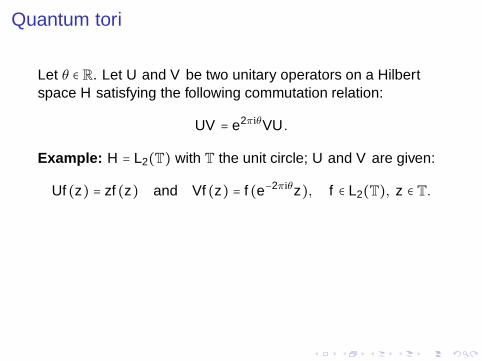
Let θ ∈ R. Let U and V be two unitary operators on a Hilbertspace H satisfying the following commutation relation:
UV = e2πiθVU.
Example: H = L2(T) with T the unit circle; U and V are given:
Uf (z) = zf (z) and Vf (z) = f (e−2πiθz), f ∈ L2(T), z ∈ T.
Quantum tori
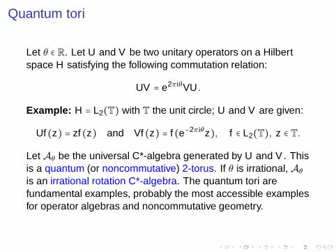
Let θ ∈ R. Let U and V be two unitary operators on a Hilbertspace H satisfying the following commutation relation:
UV = e2πiθVU.
Example: H = L2(T) with T the unit circle; U and V are given:
Uf (z) = zf (z) and Vf (z) = f (e−2πiθz), f ∈ L2(T), z ∈ T.
Let Aθ be the universal C*-algebra generated by U and V . Thisis a quantum (or noncommutative) 2-torus. If θ is irrational, Aθ
is an irrational rotation C*-algebra. The quantum tori arefundamental examples, probably the most accessible examplesfor operator algebras and noncommutative geometry.
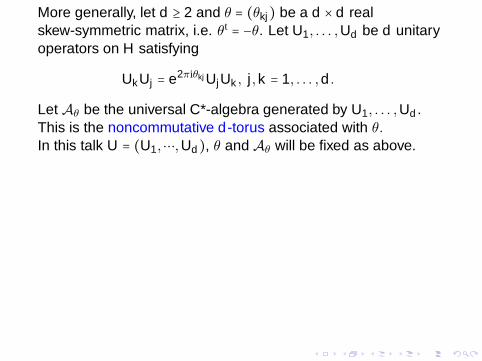
More generally, let d ≥ 2 and θ = (θkj) be a d × d realskew-symmetric matrix, i.e. θt = −θ. Let U1, . . . ,Ud be d unitaryoperators on H satisfying
UkUj = e2πiθkj UjUk , j ,k = 1, . . . ,d .
Let Aθ be the universal C*-algebra generated by U1, . . . ,Ud .This is the noncommutative d -torus associated with θ.
In this talk U = (U1,⋯,Ud), θ and Aθ will be fixed as above.
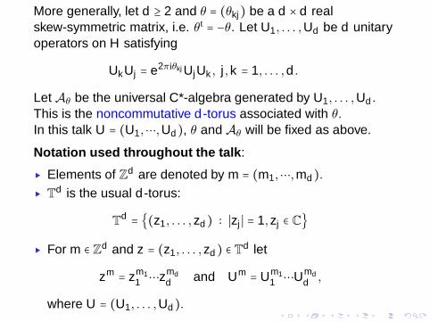
Notation used throughout the talk :
▸ Elements of Zd are denoted by m = (m1,⋯,md).▸ T
d is the usual d -torus:
Td = {(z1, . . . ,zd) ∶ ∣zj ∣ = 1,zj ∈ C}
▸ For m ∈ Zd and z = (z1, . . . ,zd) ∈ Td let
zm = zm11 ⋯zmd
d and Um = Um11 ⋯Umd
d ,
where U = (U1, . . . ,Ud).
Trace - noncommutative measure
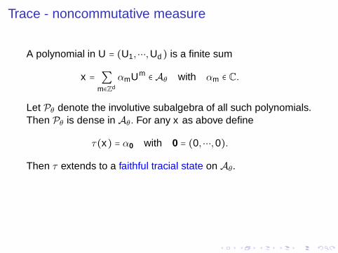
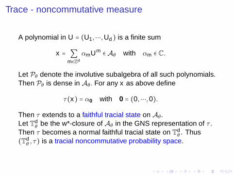
A polynomial in U = (U1,⋯,Ud) is a finite sum
x = ∑m∈Zd
αmUm ∈ Aθ with αm ∈ C.
Let Pθ denote the involutive subalgebra of all such polynomials.Then Pθ is dense in Aθ. For any x as above define
τ(x) = α0 with 0 = (0,⋯,0).
Then τ extends to a faithful tracial state on Aθ.
Trace - noncommutative measure
A polynomial in U = (U1,⋯,Ud) is a finite sum
x = ∑m∈Zd
αmUm ∈ Aθ with αm ∈ C.
Let Pθ denote the involutive subalgebra of all such polynomials.Then Pθ is dense in Aθ. For any x as above define
τ(x) = α0 with 0 = (0,⋯,0).
Then τ extends to a faithful tracial state on Aθ.Let Td
θ be the w*-closure of Aθ in the GNS representation of τ .Then τ becomes a normal faithful tracial state on T
dθ . Thus
(Tdθ , τ) is a tracial noncommutative probability space.
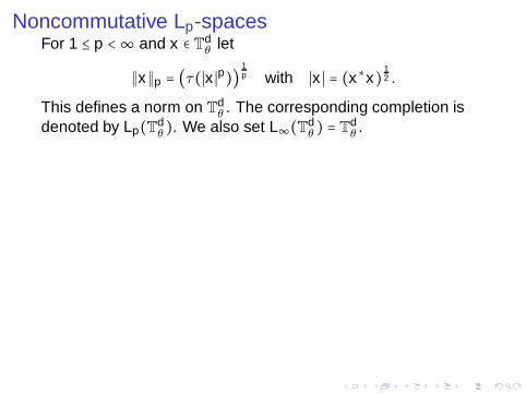
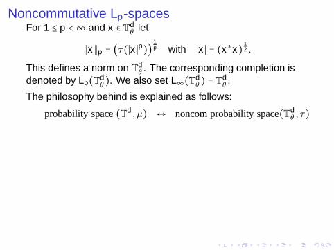
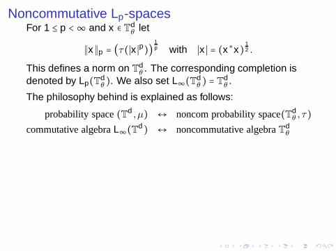
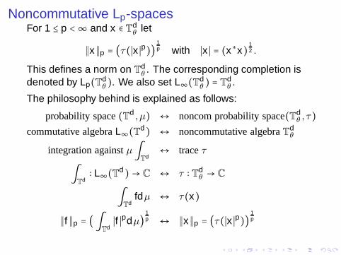
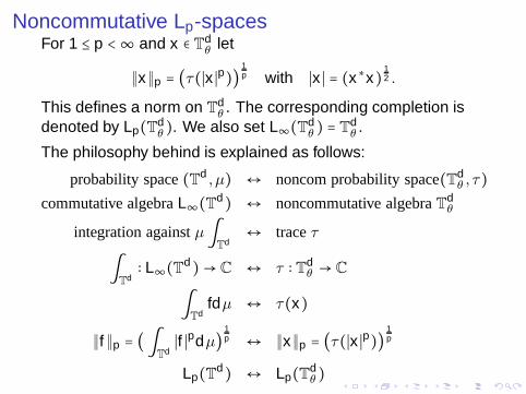
Noncommutative Lp-spacesFor 1 ≤ p < ∞ and x ∈ Td
θ let
∥x∥p = (τ(∣x ∣p))1p with ∣x ∣ = (x∗x)
12 .
This defines a norm on Tdθ . The corresponding completion is
denoted by Lp(Tdθ ). We also set L∞(Td
θ ) = Tdθ .
Noncommutative Lp-spacesFor 1 ≤ p < ∞ and x ∈ Td
θ let
∥x∥p = (τ(∣x ∣p))1p with ∣x ∣ = (x∗x)
12 .
This defines a norm on Tdθ . The corresponding completion is
denoted by Lp(Tdθ ). We also set L∞(Td
θ ) = Tdθ .
The philosophy behind is explained as follows:
probability space (Td , µ) ↔ noncom probability space(Tdθ , τ)
commutative algebra L∞(Td) ↔ noncommutative algebra Tdθ
Noncommutative Lp-spacesFor 1 ≤ p < ∞ and x ∈ Td
θ let
∥x∥p = (τ(∣x ∣p))1p with ∣x ∣ = (x∗x)
12 .
This defines a norm on Tdθ . The corresponding completion is
denoted by Lp(Tdθ ). We also set L∞(Td
θ ) = Tdθ .
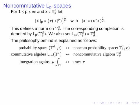
The philosophy behind is explained as follows:
probability space (Td , µ) ↔ noncom probability space(Tdθ , τ)
commutative algebra L∞(Td) ↔ noncommutative algebra Tdθ
integration against µ∫Td↔ trace τ
Noncommutative Lp-spacesFor 1 ≤ p < ∞ and x ∈ Td
θ let
∥x∥p = (τ(∣x ∣p))1p with ∣x ∣ = (x∗x)
12 .
This defines a norm on Tdθ . The corresponding completion is
denoted by Lp(Tdθ ). We also set L∞(Td
θ ) = Tdθ .
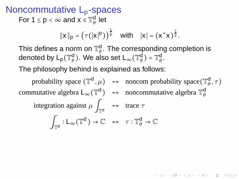
The philosophy behind is explained as follows:
probability space (Td , µ) ↔ noncom probability space(Tdθ , τ)
commutative algebra L∞(Td) ↔ noncommutative algebra Tdθ
integration against µ∫Td↔ trace τ
∫Td∶ L∞(Td)→ C ↔ τ ∶ Td
θ → C
Noncommutative Lp-spacesFor 1 ≤ p < ∞ and x ∈ Td
θ let
∥x∥p = (τ(∣x ∣p))1p with ∣x ∣ = (x∗x)
12 .
This defines a norm on Tdθ . The corresponding completion is
denoted by Lp(Tdθ ). We also set L∞(Td
θ ) = Tdθ .
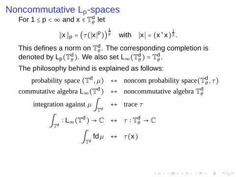
The philosophy behind is explained as follows:
probability space (Td , µ) ↔ noncom probability space(Tdθ , τ)
commutative algebra L∞(Td) ↔ noncommutative algebra Tdθ
integration against µ∫Td↔ trace τ
∫Td∶ L∞(Td)→ C ↔ τ ∶ Td
θ → C
∫Td
fdµ ↔ τ(x)
Noncommutative Lp-spacesFor 1 ≤ p < ∞ and x ∈ Td
θ let
∥x∥p = (τ(∣x ∣p))1p with ∣x ∣ = (x∗x)
12 .
This defines a norm on Tdθ . The corresponding completion is
denoted by Lp(Tdθ ). We also set L∞(Td
θ ) = Tdθ .
The philosophy behind is explained as follows:
probability space (Td , µ) ↔ noncom probability space(Tdθ , τ)
commutative algebra L∞(Td) ↔ noncommutative algebra Tdθ
integration against µ∫Td↔ trace τ
∫Td∶ L∞(Td)→ C ↔ τ ∶ Td
θ → C
∫Td
fdµ ↔ τ(x)
∥f ∥p = (∫Td∣f ∣pdµ)
1p ↔ ∥x∥p = (τ(∣x ∣p))
1p
Lp(Td) ↔ Lp(Tdθ )
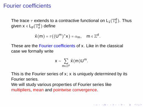
Fourier coefficients
The trace τ extends to a contractive functional on L1(Tdθ ). Thus
given x ∈ Lp(Tdθ ) define
x(m) = τ((Um)∗x) = αm, m ∈ Zd .
These are the Fourier coefficients of x . Like in the classicalcase we formally write
x ∼ ∑m∈Zd
x(m)Um.
This is the Fourier series of x ; x is uniquely determined by itsFourier series.We will study various properties of Fourier series likemultipliers, mean and pointwise convergence.
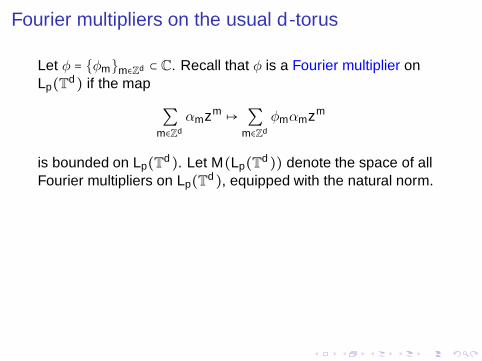
Fourier multipliers on the usual d-torus
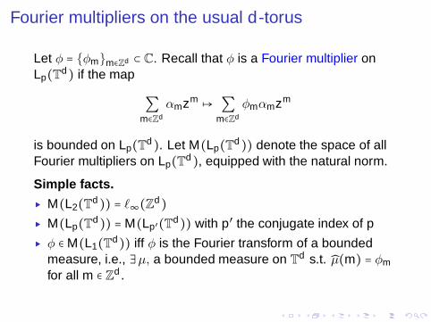
Let φ = {φm}m∈Zd ⊂ C. Recall that φ is a Fourier multiplier onLp(Td) if the map
∑m∈Zd
αmzm ↦ ∑m∈Zd
φmαmzm
is bounded on Lp(Td). Let M(Lp(Td)) denote the space of allFourier multipliers on Lp(Td), equipped with the natural norm.
Fourier multipliers on the usual d-torus
Let φ = {φm}m∈Zd ⊂ C. Recall that φ is a Fourier multiplier onLp(Td) if the map
∑m∈Zd
αmzm ↦ ∑m∈Zd
φmαmzm
is bounded on Lp(Td). Let M(Lp(Td)) denote the space of allFourier multipliers on Lp(Td), equipped with the natural norm.
Simple facts.
▸ M(L2(Td)) = ℓ∞(Zd)▸ M(Lp(Td)) =M(Lp′(Td)) with p′ the conjugate index of p
▸ φ ∈M(L1(Td)) iff φ is the Fourier transform of a boundedmeasure, i.e., ∃µ, a bounded measure on T
d s.t. µ(m) = φm
for all m ∈ Zd .
Completely bounded multipliers
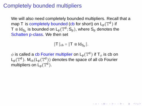
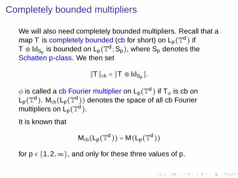
We will also need completely bounded multipliers. Recall that amap T is completely bounded (cb for short) on Lp(Td) ifT ⊗ IdSp is bounded on Lp(Td ;Sp), where Sp denotes theSchatten p-class. We then set
∥T ∥cb = ∥T ⊗ IdSp∥.
φ is called a cb Fourier multiplier on Lp(Td) if Tφ is cb onLp(Td). Mcb(Lp(Td)) denotes the space of all cb Fouriermultipliers on Lp(Td).
Completely bounded multipliers
We will also need completely bounded multipliers. Recall that amap T is completely bounded (cb for short) on Lp(Td) ifT ⊗ IdSp is bounded on Lp(Td ;Sp), where Sp denotes theSchatten p-class. We then set
∥T ∥cb = ∥T ⊗ IdSp∥.
φ is called a cb Fourier multiplier on Lp(Td) if Tφ is cb onLp(Td). Mcb(Lp(Td)) denotes the space of all cb Fouriermultipliers on Lp(Td).
It is known that
Mcb(Lp(Td)) =M(Lp(Td))
for p ∈ {1,2,∞}, and only for these three values of p.
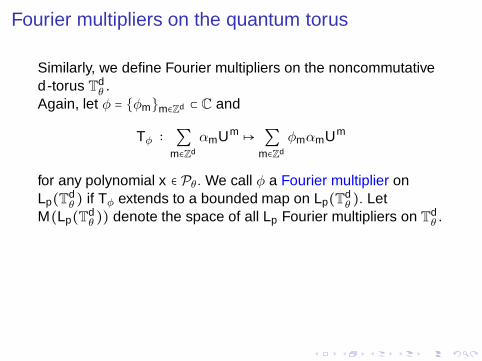
Fourier multipliers on the quantum torus
Similarly, we define Fourier multipliers on the noncommutatived -torus T
dθ .
Again, let φ = {φm}m∈Zd ⊂ C and
Tφ ∶ ∑m∈Zd
αmUm ↦ ∑m∈Zd
φmαmUm
for any polynomial x ∈ Pθ. We call φ a Fourier multiplier onLp(Td
θ ) if Tφ extends to a bounded map on Lp(Tdθ ). Let
M(Lp(Tdθ )) denote the space of all Lp Fourier multipliers on T
dθ .
Similarly, we define cb Fourier multipliers on Lp(Tdθ ) and
introduce the corresponding space Mcb(Lp(Tdθ )).
Recall that Tφ is cb on Lp(Tdθ ) if Id⊗ T is bounded on
Lp(B(ℓ2)⊗Tdθ ).
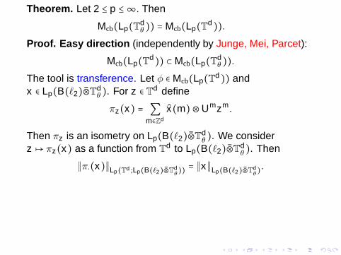
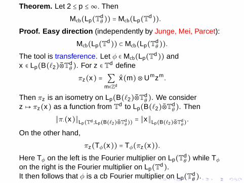
Theorem. Let 2 ≤ p ≤ ∞. Then
Mcb(Lp(Tdθ )) =Mcb(Lp(Td)).
Theorem. Let 2 ≤ p ≤ ∞. Then
Mcb(Lp(Tdθ )) =Mcb(Lp(Td)).
Proof. Easy direction (independently by Junge, Mei, Parcet):
Mcb(Lp(Td)) ⊂Mcb(Lp(Tdθ )).
The tool is transference.
Theorem. Let 2 ≤ p ≤ ∞. Then
Mcb(Lp(Tdθ )) =Mcb(Lp(Td)).
Proof. Easy direction (independently by Junge, Mei, Parcet):
Mcb(Lp(Td)) ⊂Mcb(Lp(Tdθ )).
The tool is transference. Let φ ∈Mcb(Lp(Td)) andx ∈ Lp(B(ℓ2)⊗Td
θ ). For z ∈ Td define
πz(x) = ∑m∈Zd
x(m) ⊗Umzm.
Then πz is an isometry on Lp(B(ℓ2)⊗Tdθ ).
Theorem. Let 2 ≤ p ≤ ∞. Then
Mcb(Lp(Tdθ )) =Mcb(Lp(Td)).
Proof. Easy direction (independently by Junge, Mei, Parcet):
Mcb(Lp(Td)) ⊂Mcb(Lp(Tdθ )).
The tool is transference. Let φ ∈Mcb(Lp(Td)) andx ∈ Lp(B(ℓ2)⊗Td
θ ). For z ∈ Td define
πz(x) = ∑m∈Zd
x(m) ⊗Umzm.
Then πz is an isometry on Lp(B(ℓ2)⊗Tdθ ). We consider
z ↦ πz(x) as a function from Td to Lp(B(ℓ2)⊗Td
θ ). Then
∥π⋅(x)∥Lp(Td ;Lp(B(ℓ2)⊗Tdθ)) = ∥x∥Lp(B(ℓ2)⊗T
dθ).
On the other hand,
πz(Tφ(x)) = Tφ(πz(x)).
Here Tφ on the left is the Fourier multiplier on Lp(Tdθ ) while Tφ
on the right is the Fourier multiplier on Lp(Td).It then follows that φ is a cb Fourier multiplier on Lp(Td
θ ).
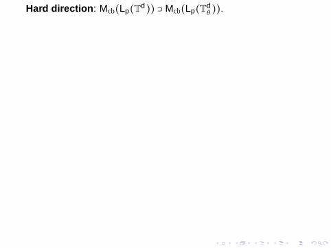
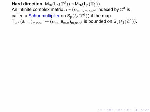
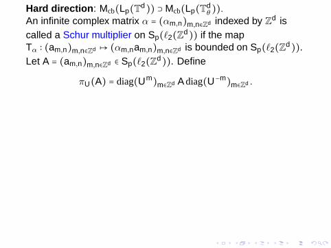
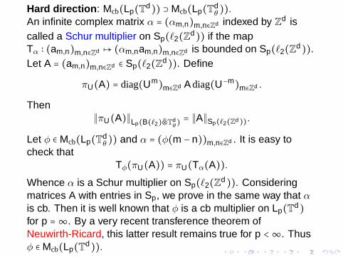
Hard direction : Mcb(Lp(Td)) ⊃Mcb(Lp(Tdθ )).
Hard direction : Mcb(Lp(Td)) ⊃Mcb(Lp(Tdθ )).
An infinite complex matrix α = (αm,n)m,n∈Zd indexed by Zd is
called a Schur multiplier on Sp(ℓ2(Zd)) if the mapTα ∶ (am,n)m,n∈Zd ↦ (αm,nam,n)m,n∈Zd is bounded on Sp(ℓ2(Zd)).
Hard direction : Mcb(Lp(Td)) ⊃Mcb(Lp(Tdθ )).
An infinite complex matrix α = (αm,n)m,n∈Zd indexed by Zd is
called a Schur multiplier on Sp(ℓ2(Zd)) if the mapTα ∶ (am,n)m,n∈Zd ↦ (αm,nam,n)m,n∈Zd is bounded on Sp(ℓ2(Zd)).Let A = (am,n)m,n∈Zd ∈ Sp(ℓ2(Zd)). Define
πU(A) = diag(Um)m∈Zd A diag(U−m)m∈Zd .
Hard direction : Mcb(Lp(Td)) ⊃Mcb(Lp(Tdθ )).
An infinite complex matrix α = (αm,n)m,n∈Zd indexed by Zd is
called a Schur multiplier on Sp(ℓ2(Zd)) if the mapTα ∶ (am,n)m,n∈Zd ↦ (αm,nam,n)m,n∈Zd is bounded on Sp(ℓ2(Zd)).Let A = (am,n)m,n∈Zd ∈ Sp(ℓ2(Zd)). Define
πU(A) = diag(Um)m∈Zd A diag(U−m)m∈Zd .
Then∥πU(A)∥Lp(B(ℓ2)⊗T
dθ) = ∥A∥Sp(ℓ2(Zd)).
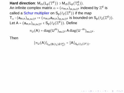
Let φ ∈Mcb(Lp(Tdθ )) and α = (φ(m − n))m,n∈Zd . It is easy to
check thatTφ(πU(A)) = πU(Tα(A)).
Whence α is a Schur multiplier on Sp(ℓ2(Zd)).
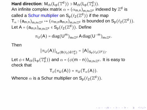
Hard direction : Mcb(Lp(Td)) ⊃Mcb(Lp(Tdθ )).
An infinite complex matrix α = (αm,n)m,n∈Zd indexed by Zd is
called a Schur multiplier on Sp(ℓ2(Zd)) if the mapTα ∶ (am,n)m,n∈Zd ↦ (αm,nam,n)m,n∈Zd is bounded on Sp(ℓ2(Zd)).Let A = (am,n)m,n∈Zd ∈ Sp(ℓ2(Zd)). Define
πU(A) = diag(Um)m∈Zd A diag(U−m)m∈Zd .
Then∥πU(A)∥Lp(B(ℓ2)⊗T
dθ) = ∥A∥Sp(ℓ2(Zd)).
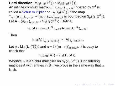
Let φ ∈Mcb(Lp(Tdθ )) and α = (φ(m − n))m,n∈Zd . It is easy to
check thatTφ(πU(A)) = πU(Tα(A)).
Whence α is a Schur multiplier on Sp(ℓ2(Zd)). Consideringmatrices A with entries in Sp, we prove in the same way that αis cb.
Hard direction : Mcb(Lp(Td)) ⊃Mcb(Lp(Tdθ )).
An infinite complex matrix α = (αm,n)m,n∈Zd indexed by Zd is
called a Schur multiplier on Sp(ℓ2(Zd)) if the mapTα ∶ (am,n)m,n∈Zd ↦ (αm,nam,n)m,n∈Zd is bounded on Sp(ℓ2(Zd)).Let A = (am,n)m,n∈Zd ∈ Sp(ℓ2(Zd)). Define
πU(A) = diag(Um)m∈Zd A diag(U−m)m∈Zd .
Then∥πU(A)∥Lp(B(ℓ2)⊗T
dθ) = ∥A∥Sp(ℓ2(Zd)).
Let φ ∈Mcb(Lp(Tdθ )) and α = (φ(m − n))m,n∈Zd . It is easy to
check thatTφ(πU(A)) = πU(Tα(A)).
Whence α is a Schur multiplier on Sp(ℓ2(Zd)). Consideringmatrices A with entries in Sp, we prove in the same way that αis cb. Then it is well known that φ is a cb multiplier on Lp(Td)for p = ∞. By a very recent transference theorem ofNeuwirth-Ricard, this latter result remains true for p < ∞. Thusφ ∈Mcb(Lp(Td)).
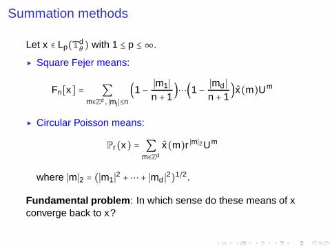
Summation methods
Let x ∈ Lp(Tdθ ) with 1 ≤ p ≤ ∞.
▸ Square Fejer means:
Fn[x] = ∑m∈Zd , ∣mj ∣≤n
(1 − ∣m1∣n + 1
)⋯(1 − ∣md ∣n + 1
)x(m)Um
▸ Circular Poisson means:
Pr(x) = ∑m∈Zd
x(m)r ∣m∣2Um
where ∣m∣2 = (∣m1∣2 +⋯+ ∣md ∣2)1/2.
Fundamental problem : In which sense do these means of xconverge back to x?
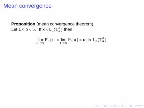
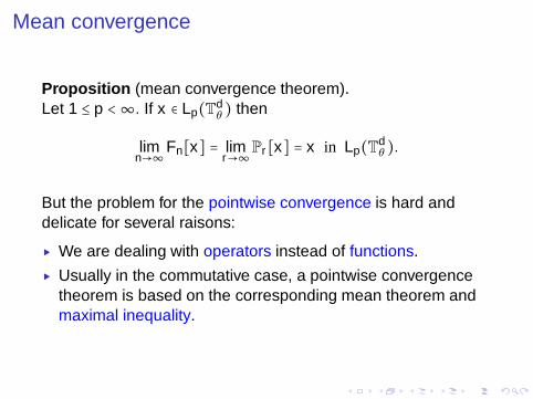
Mean convergence
Proposition (mean convergence theorem).Let 1 ≤ p < ∞. If x ∈ Lp(Td
θ ) then
limn→∞
Fn[x] = limr→∞
Pr [x] = x in Lp(Tdθ ).
Mean convergence
Proposition (mean convergence theorem).Let 1 ≤ p < ∞. If x ∈ Lp(Td
θ ) then
limn→∞
Fn[x] = limr→∞
Pr [x] = x in Lp(Tdθ ).
But the problem for the pointwise convergence is hard anddelicate for several raisons:
▸ We are dealing with operators instead of functions.
▸ Usually in the commutative case, a pointwise convergencetheorem is based on the corresponding mean theorem andmaximal inequality.
Pointwise convergence
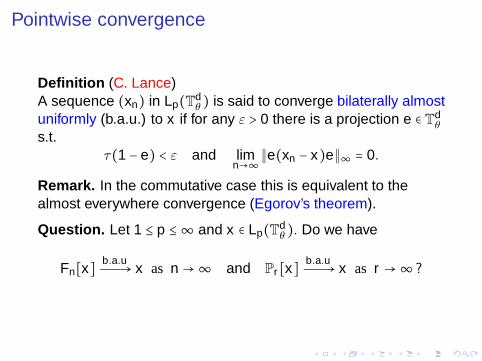
Definition (C. Lance)A sequence (xn) in Lp(Td
θ ) is said to converge bilaterally almostuniformly (b.a.u.) to x if for any ε > 0 there is a projection e ∈ Td
θ
s.t.τ(1 − e) < ε and lim
n→∞∥e(xn − x)e∥∞ = 0.
Remark. In the commutative case this is equivalent to thealmost everywhere convergence (Egorov’s theorem).
Question. Let 1 ≤ p ≤ ∞ and x ∈ Lp(Tdθ ). Do we have
Fn[x] b.a.uÐÐ→ x as n →∞ and Pr [x] b.a.uÐÐ→ x as r →∞?
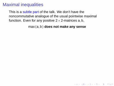
Maximal inequalities
This is a subtle part of the talk. We don’t have thenoncommutative analogue of the usual pointwise maximalfunction. Even for any positive 2 × 2-matrices a,b,
max(a,b) does not make any sense
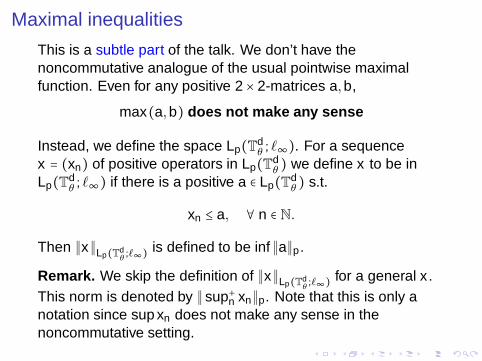
Maximal inequalities
This is a subtle part of the talk. We don’t have thenoncommutative analogue of the usual pointwise maximalfunction. Even for any positive 2 × 2-matrices a,b,
max(a,b) does not make any sense
Instead, we define the space Lp(Tdθ ; ℓ∞). For a sequence
x = (xn) of positive operators in Lp(Tdθ ) we define x to be in
Lp(Tdθ ; ℓ∞) if there is a positive a ∈ Lp(Td
θ ) s.t.
xn ≤ a, ∀ n ∈ N.
Then ∥x∥Lp(Tdθ;ℓ∞)
is defined to be inf ∥a∥p.
Remark. We skip the definition of ∥x∥Lp(Tdθ;ℓ∞)
for a general x .This norm is denoted by ∥sup+n xn∥p. Note that this is only anotation since sup xn does not make any sense in thenoncommutative setting.
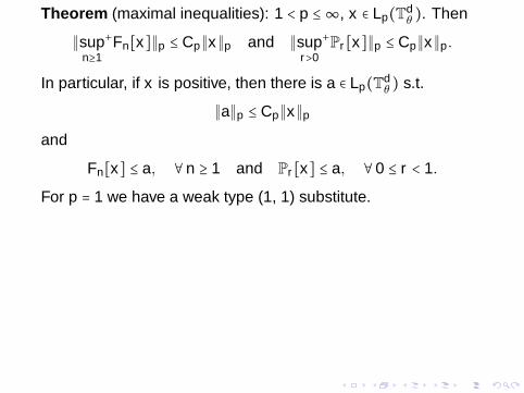
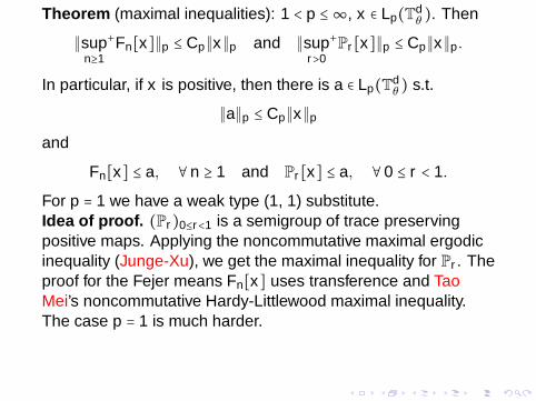
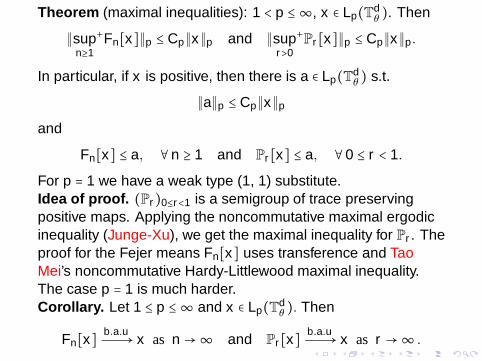
Theorem (maximal inequalities): 1 < p ≤ ∞, x ∈ Lp(Tdθ ). Then
∥supn≥1
+Fn[x]∥p ≤ Cp∥x∥p and ∥supr>0
+Pr [x]∥p ≤ Cp∥x∥p.
In particular, if x is positive, then there is a ∈ Lp(Tdθ ) s.t.
∥a∥p ≤ Cp∥x∥pand
Fn[x] ≤ a, ∀n ≥ 1 and Pr [x] ≤ a, ∀0 ≤ r < 1.
For p = 1 we have a weak type (1, 1) substitute.
Theorem (maximal inequalities): 1 < p ≤ ∞, x ∈ Lp(Tdθ ). Then
∥supn≥1
+Fn[x]∥p ≤ Cp∥x∥p and ∥supr>0
+Pr [x]∥p ≤ Cp∥x∥p.
In particular, if x is positive, then there is a ∈ Lp(Tdθ ) s.t.
∥a∥p ≤ Cp∥x∥pand
Fn[x] ≤ a, ∀n ≥ 1 and Pr [x] ≤ a, ∀0 ≤ r < 1.
For p = 1 we have a weak type (1, 1) substitute.Idea of proof. (Pr)0≤r<1 is a semigroup of trace preservingpositive maps. Applying the noncommutative maximal ergodicinequality (Junge-Xu), we get the maximal inequality for Pr . Theproof for the Fejer means Fn[x] uses transference and TaoMei’s noncommutative Hardy-Littlewood maximal inequality.The case p = 1 is much harder.
Theorem (maximal inequalities): 1 < p ≤ ∞, x ∈ Lp(Tdθ ). Then
∥supn≥1
+Fn[x]∥p ≤ Cp∥x∥p and ∥supr>0
+Pr [x]∥p ≤ Cp∥x∥p.
In particular, if x is positive, then there is a ∈ Lp(Tdθ ) s.t.
∥a∥p ≤ Cp∥x∥pand
Fn[x] ≤ a, ∀n ≥ 1 and Pr [x] ≤ a, ∀0 ≤ r < 1.
For p = 1 we have a weak type (1, 1) substitute.Idea of proof. (Pr)0≤r<1 is a semigroup of trace preservingpositive maps. Applying the noncommutative maximal ergodicinequality (Junge-Xu), we get the maximal inequality for Pr . Theproof for the Fejer means Fn[x] uses transference and TaoMei’s noncommutative Hardy-Littlewood maximal inequality.The case p = 1 is much harder.Corollary. Let 1 ≤ p ≤ ∞ and x ∈ Lp(Td
θ ). Then
Fn[x] b.a.uÐÐ→ x as n →∞ and Pr [x] b.a.uÐÐ→ x as r →∞ .
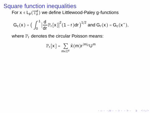
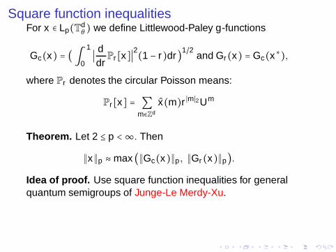
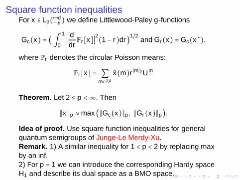
Square function inequalitiesFor x ∈ Lp(Td
θ ) we define Littlewood-Paley g-functions
Gc(x) = (∫1
0∣ ddr
Pr [x]∣2(1 − r)dr)1/2 and Gr(x) = Gc(x∗),
where Pr denotes the circular Poisson means:
Pr [x] = ∑m∈Zd
x(m)r ∣m∣2Um
Square function inequalitiesFor x ∈ Lp(Td
θ ) we define Littlewood-Paley g-functions
Gc(x) = (∫1
0∣ ddr
Pr [x]∣2(1 − r)dr)1/2 and Gr(x) = Gc(x∗),
where Pr denotes the circular Poisson means:
Pr [x] = ∑m∈Zd
x(m)r ∣m∣2Um
Theorem. Let 2 ≤ p < ∞. Then
∥x∥p ≈max (∥Gc(x)∥p, ∥Gr(x)∥p).
Idea of proof. Use square function inequalities for generalquantum semigroups of Junge-Le Merdy-Xu.
Square function inequalitiesFor x ∈ Lp(Td
θ ) we define Littlewood-Paley g-functions
Gc(x) = (∫1
0∣ ddr
Pr [x]∣2(1 − r)dr)1/2 and Gr(x) = Gc(x∗),
where Pr denotes the circular Poisson means:
Pr [x] = ∑m∈Zd
x(m)r ∣m∣2Um
Theorem. Let 2 ≤ p < ∞. Then
∥x∥p ≈max (∥Gc(x)∥p, ∥Gr(x)∥p).
Idea of proof. Use square function inequalities for generalquantum semigroups of Junge-Le Merdy-Xu.Remark. 1) A similar inequality for 1 < p < 2 by replacing maxby an inf.2) For p = 1 we can introduce the corresponding Hardy spaceH1 and describe its dual space as a BMO space.


![HITCHIN HARMONIC MAPS ARE IMMERSIONShomepages.math.uic.edu › ~andysan › HitImmersion.pdf · HITCHIN HARMONIC MAPS ARE IMMERSIONS ANDREW SANDERS ... [SY78] about harmonic maps](https://static.fdocument.org/doc/165x107/5f13addc3b5c9d385756c3dc/hitchin-harmonic-maps-are-a-andysan-a-hitimmersionpdf-hitchin-harmonic-maps.jpg)