Hardy inequalities and applications Maria J. ESTEBAN …castro/Esteban.pdf · Hardy inequalities...
56
Hardy inequalities and applications Maria J. ESTEBAN C.N.R.S. & Université Paris-Dauphine In collaboration with : Adimurthi, Roberta Bosi, Jean Dolbeault, MIchael Loss, Luis Vega Cartagena de Indias, July 2007 – p.1/18
Transcript of Hardy inequalities and applications Maria J. ESTEBAN …castro/Esteban.pdf · Hardy inequalities...
Hardy inequalities and applications
Maria J. ESTEBAN
C.N.R.S. & Université Paris-Dauphine
In collaboration with : Adimurthi, Roberta Bosi, Jean Dolbeault, MIchael Loss, Luis Vega
Cartagena de Indias, July 2007 – p.1/18
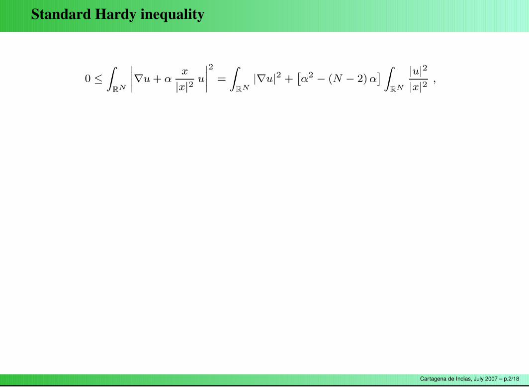
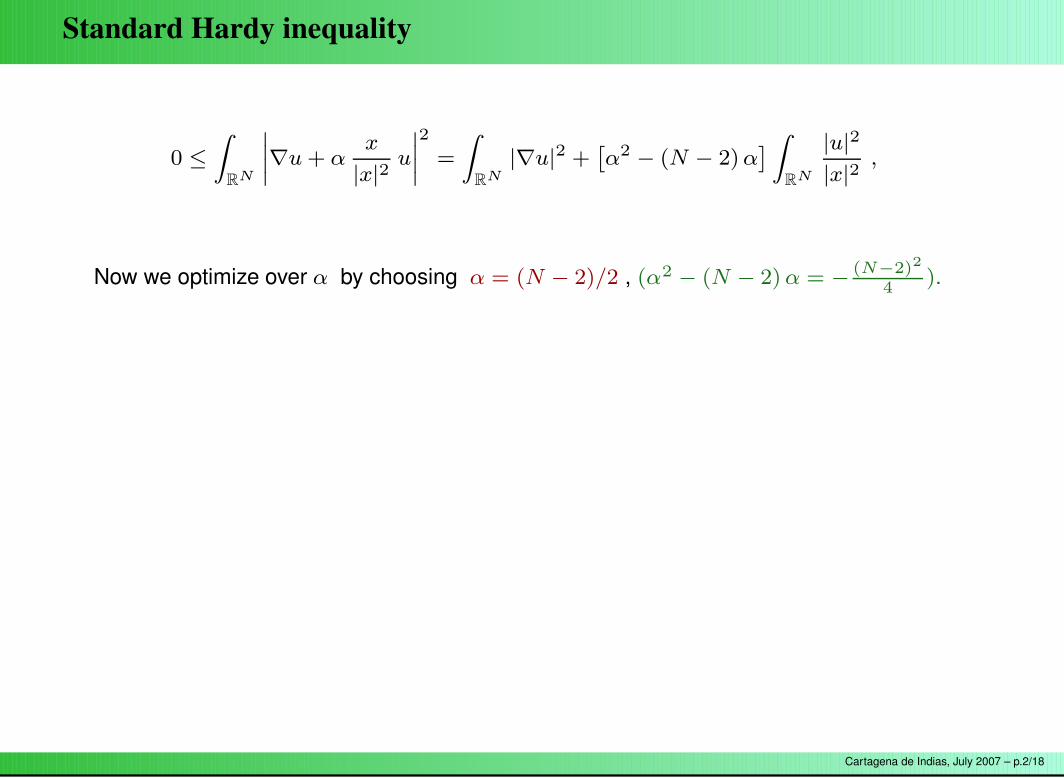
Standard Hardy inequality
0 ≤
Z
RN
˛
˛
˛
˛
∇u + αx
|x|2u
˛
˛
˛
˛
2
=
Z
RN
|∇u|2 +ˆ
α2 − (N − 2) α˜
Z
RN
|u|2
|x|2,
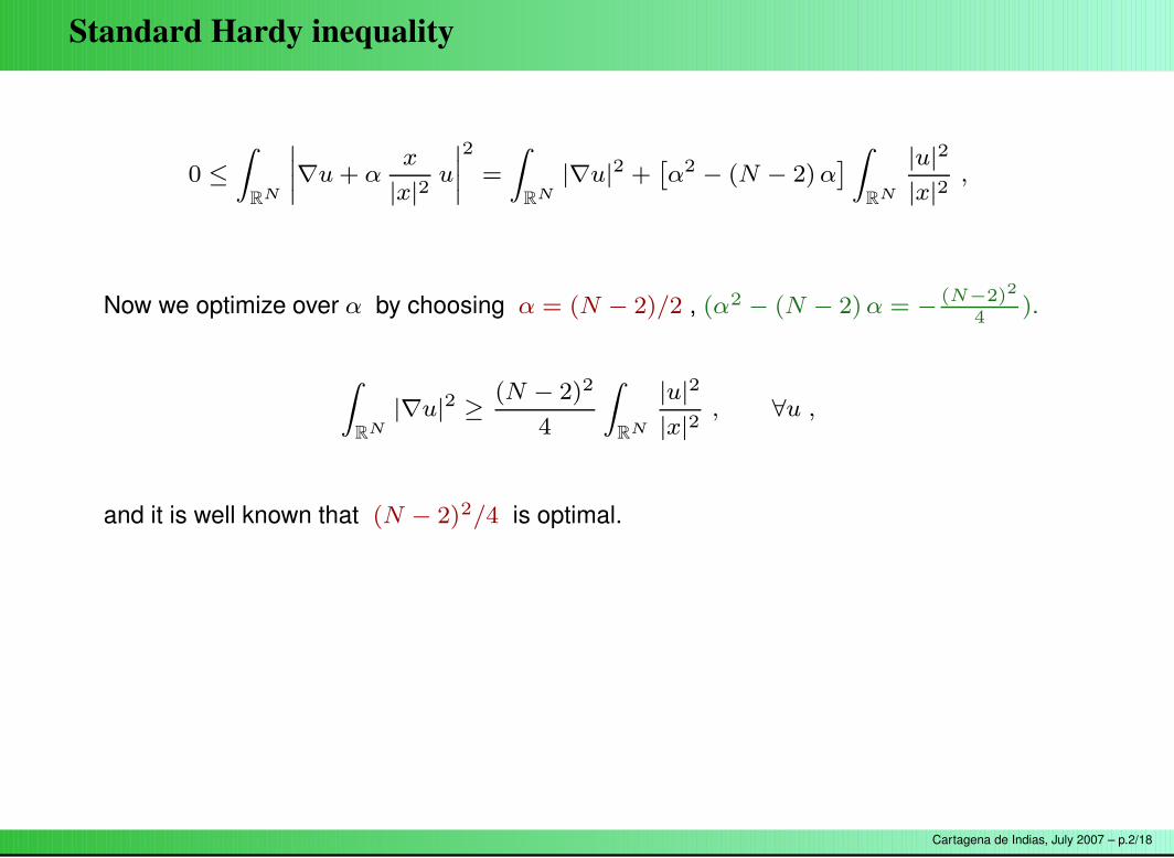
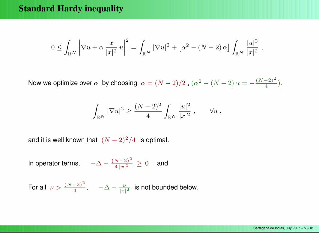
Now we optimize over α by choosing α = (N − 2)/2 , (α2 − (N − 2) α = − (N−2)2
4).
Z
RN
|∇u|2 ≥(N − 2)2
4
Z
RN
|u|2
|x|2, ∀u ,
and it is well known that (N − 2)2/4 is optimal.
In operator terms, −∆ − (N−2)2
4 |x|2≥ 0 and
For all ν >(N−2)2
4, −∆ − ν
|x|2is not bounded below.
Cartagena de Indias, July 2007 – p.2/18
Standard Hardy inequality
0 ≤
Z
RN
˛
˛
˛
˛
∇u + αx
|x|2u
˛
˛
˛
˛
2
=
Z
RN
|∇u|2 +ˆ
α2 − (N − 2) α˜
Z
RN
|u|2
|x|2,
Now we optimize over α by choosing α = (N − 2)/2 , (α2 − (N − 2) α = − (N−2)2
4).
Z
RN
|∇u|2 ≥(N − 2)2
4
Z
RN
|u|2
|x|2, ∀u ,
and it is well known that (N − 2)2/4 is optimal.
In operator terms, −∆ − (N−2)2
4 |x|2≥ 0 and
For all ν >(N−2)2
4, −∆ − ν
|x|2is not bounded below.
Cartagena de Indias, July 2007 – p.2/18
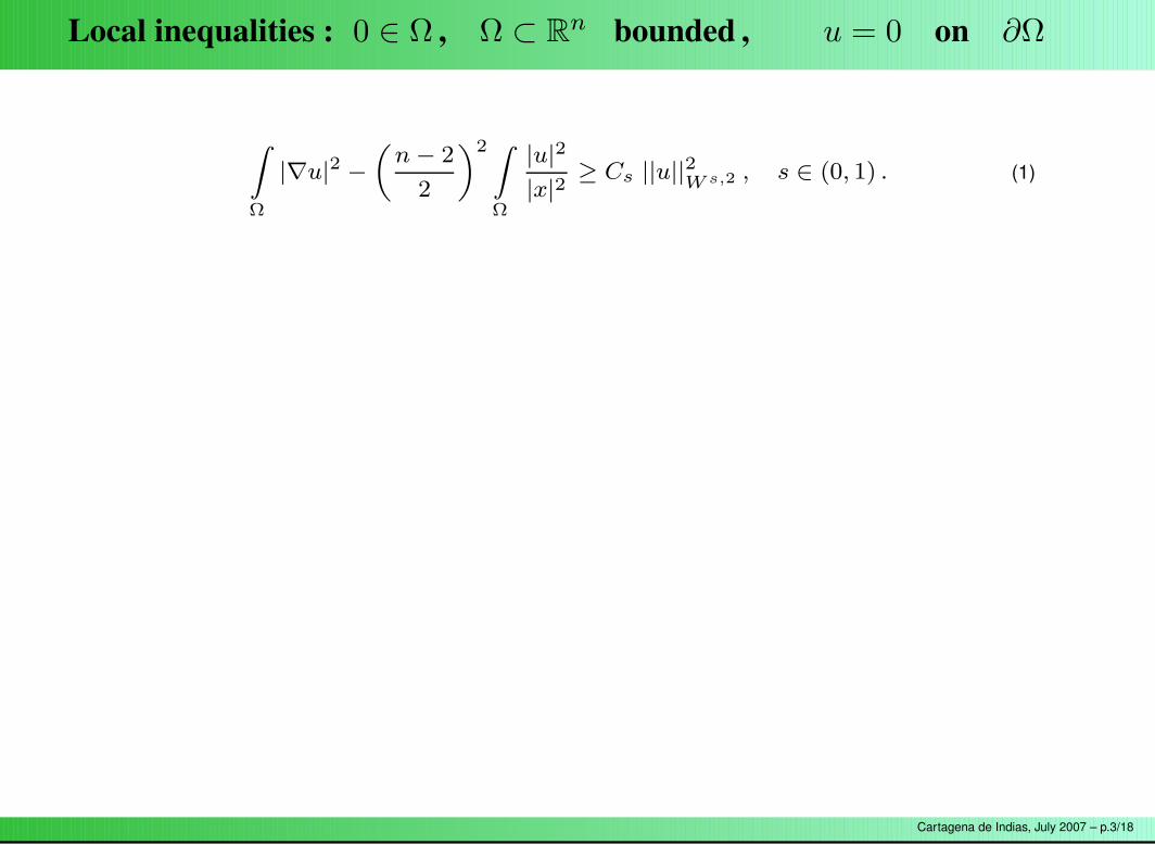
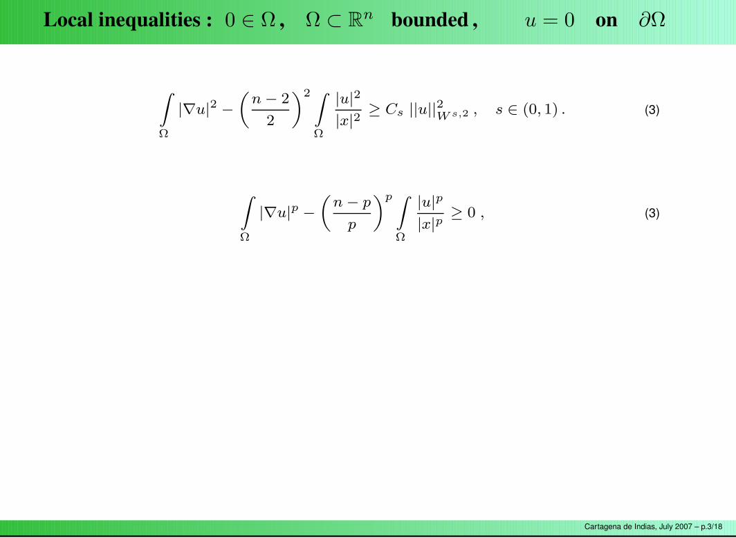
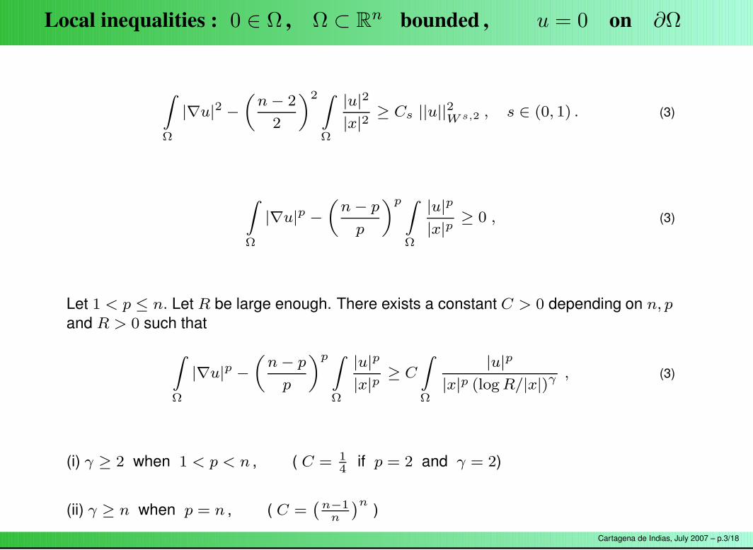
Local inequalities : 0 ∈ Ω , Ω ⊂ Rn bounded , u = 0 on ∂Ω
Z
Ω
|∇u|2 −
„
n − 2
2
«2 Z
Ω
|u|2
|x|2≥ Cs ||u||2
W s,2 , s ∈ (0, 1) . (1)
Z
Ω
|∇u|p −
„
n − p
p
«p Z
Ω
|u|p
|x|p≥ 0 , (2)
Let 1 < p ≤ n. Let R be large enough. There exists a constant C > 0 depending on n, pand R > 0 such that
Z
Ω
|∇u|p −
„
n − p
p
«p Z
Ω
|u|p
|x|p≥ C
Z
Ω
|u|p
|x|p (log R/|x|)γ , (3)
(i) γ ≥ 2 when 1 < p < n , ( C = 14
if p = 2 and γ = 2)
(ii) γ ≥ n when p = n , ( C =`
n−1n
´n )
Cartagena de Indias, July 2007 – p.3/18
Local inequalities : 0 ∈ Ω , Ω ⊂ Rn bounded , u = 0 on ∂Ω
Z
Ω
|∇u|2 −
„
n − 2
2
«2 Z
Ω
|u|2
|x|2≥ Cs ||u||2
W s,2 , s ∈ (0, 1) . (3)
Z
Ω
|∇u|p −
„
n − p
p
«p Z
Ω
|u|p
|x|p≥ 0 , (3)
Let 1 < p ≤ n. Let R be large enough. There exists a constant C > 0 depending on n, pand R > 0 such that
Z
Ω
|∇u|p −
„
n − p
p
«p Z
Ω
|u|p
|x|p≥ C
Z
Ω
|u|p
|x|p (log R/|x|)γ , (3)
(i) γ ≥ 2 when 1 < p < n , ( C = 14
if p = 2 and γ = 2)
(ii) γ ≥ n when p = n , ( C =`
n−1n
´n )
Cartagena de Indias, July 2007 – p.3/18
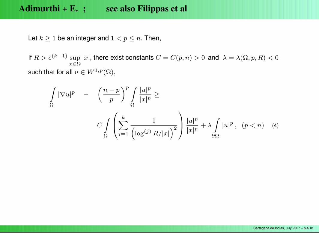
Adimurthi + E. ; see also Filippas et al
Let k ≥ 1 be an integer and 1 < p ≤ n. Then,
If R > e(k−1) supx∈Ω
|x|, there exist constants C = C(p, n) > 0 and λ = λ(Ω, p, R) < 0
such that for all u ∈ W 1,p(Ω),
Z
Ω
|∇u|p −
„
n − p
p
«p Z
Ω
|u|p
|x|p≥
C
Z
Ω
0
B
@
kX
j=1
1“
log(j) R/|x|”2
1
C
A
|u|p
|x|p+ λ
Z
∂Ω
|u|p , (p < n) (4)
Z
Ω
|∇u|n −
„
n − 1
n
«Z
Ω
|u|n“
|x| log R|x|
”n ≥
C
Z
Ω
0
@
kX
j=2
1“
log(j) R/|x|”n
1
A
|u|n
|x|n+ λ
Z
∂Ω
|u|n , (p = n) (5)
Cartagena de Indias, July 2007 – p.4/18
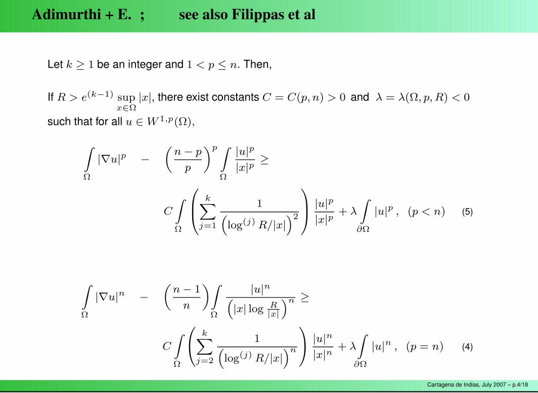
Adimurthi + E. ; see also Filippas et al
Let k ≥ 1 be an integer and 1 < p ≤ n. Then,
If R > e(k−1) supx∈Ω
|x|, there exist constants C = C(p, n) > 0 and λ = λ(Ω, p, R) < 0
such that for all u ∈ W 1,p(Ω),
Z
Ω
|∇u|p −
„
n − p
p
«p Z
Ω
|u|p
|x|p≥
C
Z
Ω
0
B
@
kX
j=1
1“
log(j) R/|x|”2
1
C
A
|u|p
|x|p+ λ
Z
∂Ω
|u|p , (p < n) (5)
Z
Ω
|∇u|n −
„
n − 1
n
«Z
Ω
|u|n“
|x| log R|x|
”n ≥
C
Z
Ω
0
@
kX
j=2
1“
log(j) R/|x|”n
1
A
|u|n
|x|n+ λ
Z
∂Ω
|u|n , (p = n) (4)
Cartagena de Indias, July 2007 – p.4/18
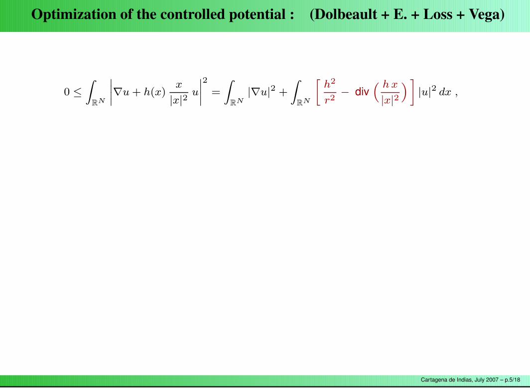
Optimization of the controlled potential : (Dolbeault + E. + Loss + Vega)
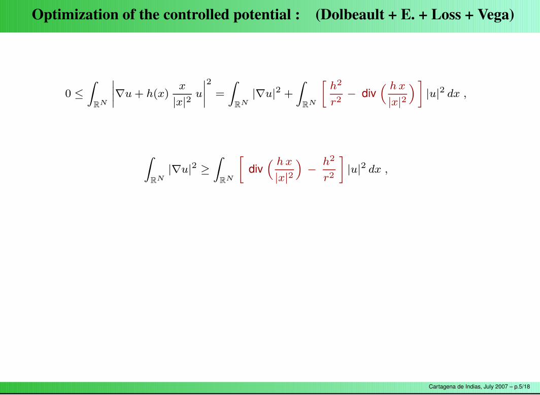
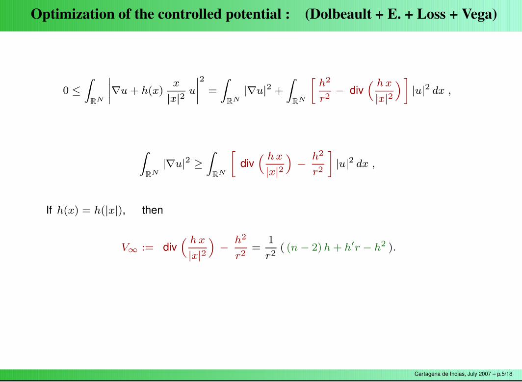
0 ≤
Z
RN
˛
˛
˛
˛
∇u + h(x)x
|x|2u
˛
˛
˛
˛
2
=
Z
RN
|∇u|2 +
Z
RN
»
h2
r2− div
“ h x
|x|2
”
–
|u|2 dx ,
Z
RN
|∇u|2 ≥
Z
RN
»
div“ h x
|x|2
”
−h2
r2
–
|u|2 dx ,
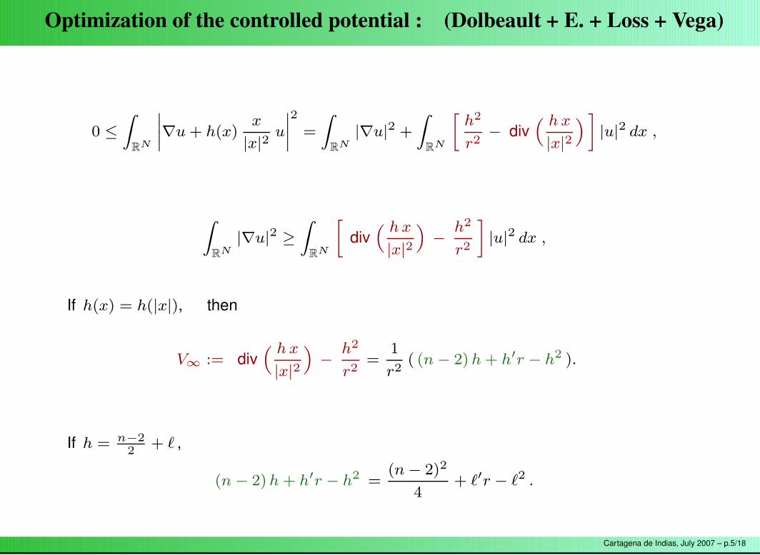
If h(x) = h(|x|), then
V∞ := div“ h x
|x|2
”
−h2
r2=
1
r2( (n − 2) h + h′r − h2 ).
If h = n−22
+ ` ,
(n − 2) h + h′r − h2 =(n − 2)2
4+ `′r − `2 .
Cartagena de Indias, July 2007 – p.5/18
Optimization of the controlled potential : (Dolbeault + E. + Loss + Vega)
0 ≤
Z
RN
˛
˛
˛
˛
∇u + h(x)x
|x|2u
˛
˛
˛
˛
2
=
Z
RN
|∇u|2 +
Z
RN
»
h2
r2− div
“ h x
|x|2
”
–
|u|2 dx ,
Z
RN
|∇u|2 ≥
Z
RN
»
div“ h x
|x|2
”
−h2
r2
–
|u|2 dx ,
If h(x) = h(|x|), then
V∞ := div“ h x
|x|2
”
−h2
r2=
1
r2( (n − 2) h + h′r − h2 ).
If h = n−22
+ ` ,
(n − 2) h + h′r − h2 =(n − 2)2
4+ `′r − `2 .
Cartagena de Indias, July 2007 – p.5/18
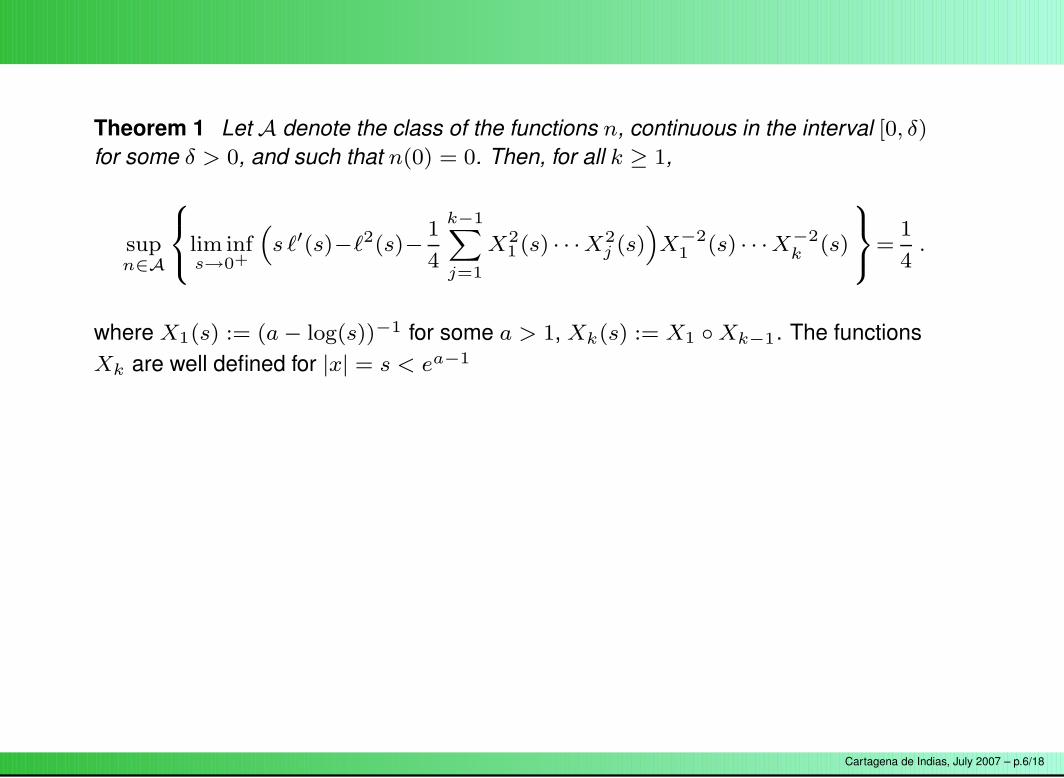
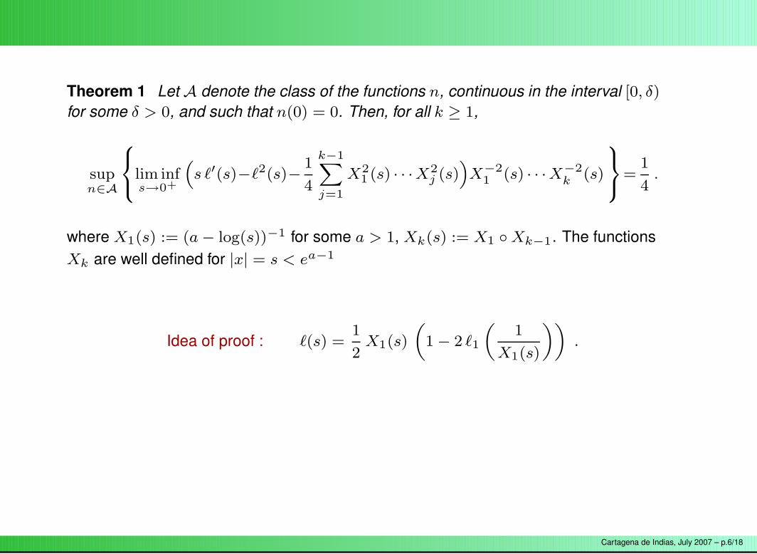
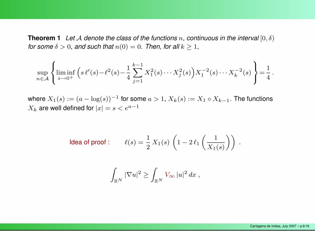
Theorem 1 Let A denote the class of the functions n, continuous in the interval [0, δ)
for some δ > 0, and such that n(0) = 0. Then, for all k ≥ 1,
supn∈A
8
<
:
lim infs→0+
“
s `′(s)−`2(s)−1
4
k−1X
j=1
X21 (s) · · ·X2
j (s)”
X−21 (s) · · ·X−2
k (s)
9
=
;
=1
4.
where X1(s) := (a − log(s))−1 for some a > 1, Xk(s) := X1 Xk−1. The functionsXk are well defined for |x| = s < ea−1
Idea of proof : `(s) =1
2X1(s)
„
1 − 2 `1
„
1
X1(s)
««
.
Z
RN
|∇u|2 ≥
Z
RN
V∞ |u|2 dx ,
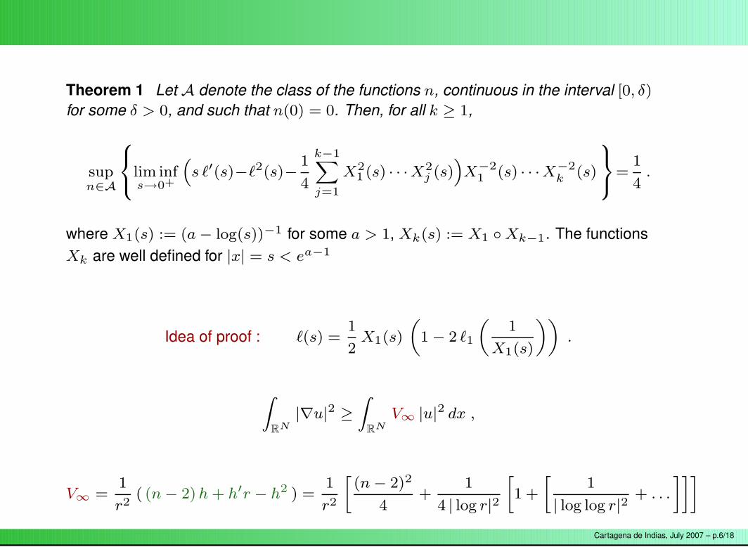
V∞ =1
r2( (n − 2) h + h′r − h2 ) =
1
r2
»
(n − 2)2
4+
1
4 | log r|2
»
1 +
»
1
| log log r|2+ . . .
–––
V∞(s) =1
4
“
1 +
+∞X
j=1
X21 (s) · · ·X2
j (s)”
. (4)
Cartagena de Indias, July 2007 – p.6/18
Theorem 1 Let A denote the class of the functions n, continuous in the interval [0, δ)
for some δ > 0, and such that n(0) = 0. Then, for all k ≥ 1,
supn∈A
8
<
:
lim infs→0+
“
s `′(s)−`2(s)−1
4
k−1X
j=1
X21 (s) · · ·X2
j (s)”
X−21 (s) · · ·X−2
k (s)
9
=
;
=1
4.
where X1(s) := (a − log(s))−1 for some a > 1, Xk(s) := X1 Xk−1. The functionsXk are well defined for |x| = s < ea−1
Idea of proof : `(s) =1
2X1(s)
„
1 − 2 `1
„
1
X1(s)
««
.
Z
RN
|∇u|2 ≥
Z
RN
V∞ |u|2 dx ,
V∞ =1
r2( (n − 2) h + h′r − h2 ) =
1
r2
»
(n − 2)2
4+
1
4 | log r|2
»
1 +
»
1
| log log r|2+ . . .
–––
V∞(s) =1
4
“
1 +
+∞X
j=1
X21 (s) · · ·X2
j (s)”
. (4)
Cartagena de Indias, July 2007 – p.6/18
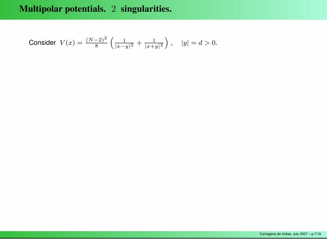
Multipolar potentials. 2 singularities.
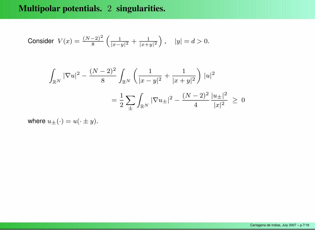
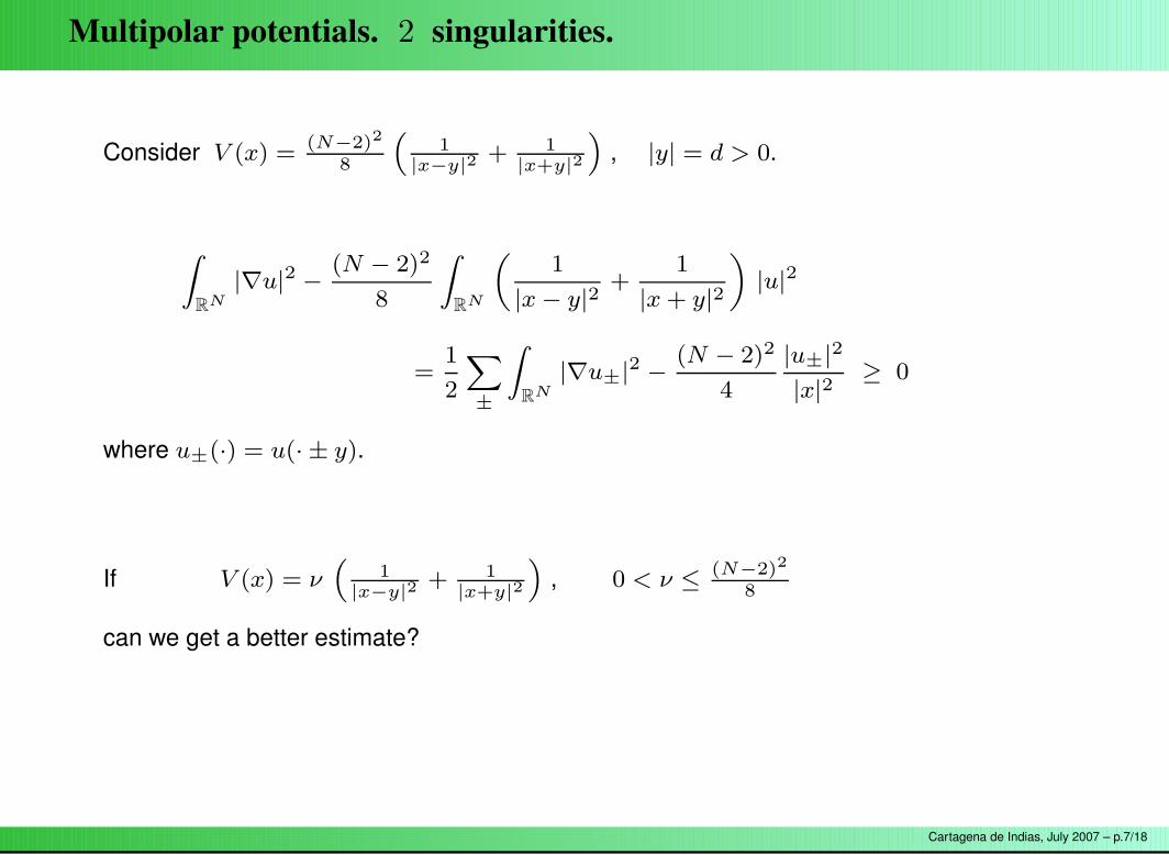
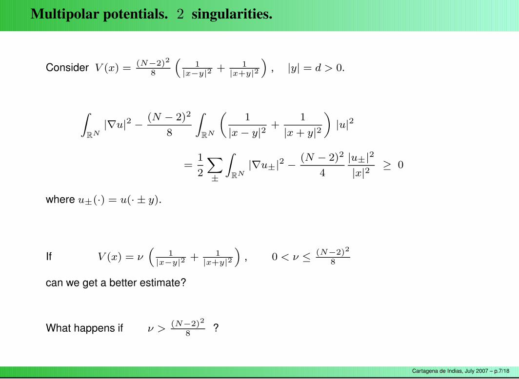
Consider V (x) =(N−2)2
8
“
1|x−y|2
+ 1|x+y|2
”
, |y| = d > 0.
Z
RN
|∇u|2 −(N − 2)2
8
Z
RN
„
1
|x − y|2+
1
|x + y|2
«
|u|2
=1
2
X
±
Z
RN
|∇u±|2 −(N − 2)2
4
|u±|2
|x|2≥ 0
where u±(·) = u(· ± y).
If V (x) = ν“
1|x−y|2
+ 1|x+y|2
”
, 0 < ν ≤ (N−2)2
8
can we get a better estimate?
What happens if ν >(N−2)2
8?
Cartagena de Indias, July 2007 – p.7/18
Multipolar potentials. 2 singularities.
Consider V (x) =(N−2)2
8
“
1|x−y|2
+ 1|x+y|2
”
, |y| = d > 0.
Z
RN
|∇u|2 −(N − 2)2
8
Z
RN
„
1
|x − y|2+
1
|x + y|2
«
|u|2
=1
2
X
±
Z
RN
|∇u±|2 −(N − 2)2
4
|u±|2
|x|2≥ 0
where u±(·) = u(· ± y).
If V (x) = ν“
1|x−y|2
+ 1|x+y|2
”
, 0 < ν ≤ (N−2)2
8
can we get a better estimate?
What happens if ν >(N−2)2
8?
Cartagena de Indias, July 2007 – p.7/18
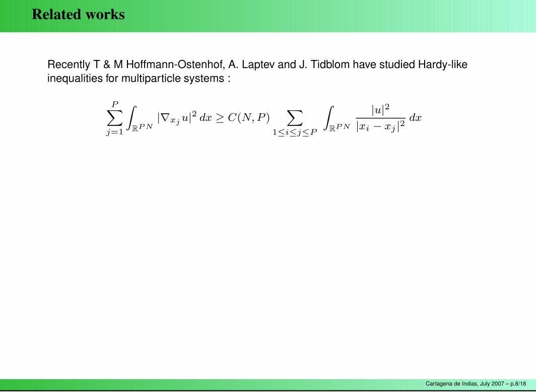
Related works
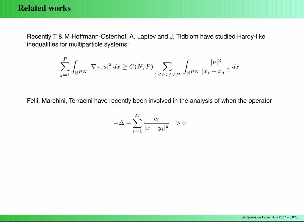
Recently T & M Hoffmann-Ostenhof, A. Laptev and J. Tidblom have studied Hardy-likeinequalities for multiparticle systems :
PX
j=1
Z
RP N
|∇xju|2 dx ≥ C(N, P )
X
1≤i≤j≤P
Z
RP N
|u|2
|xi − xj |2dx
Felli, Marchini, Terracini have recently been involved in the analysis of when the operator
−∆ −MX
i=1
ci
|x − yi|2> 0
Cartagena de Indias, July 2007 – p.8/18
Related works
Recently T & M Hoffmann-Ostenhof, A. Laptev and J. Tidblom have studied Hardy-likeinequalities for multiparticle systems :
PX
j=1
Z
RP N
|∇xju|2 dx ≥ C(N, P )
X
1≤i≤j≤P
Z
RP N
|u|2
|xi − xj |2dx
Felli, Marchini, Terracini have recently been involved in the analysis of when the operator
−∆ −MX
i=1
ci
|x − yi|2> 0
Cartagena de Indias, July 2007 – p.8/18

Spectral meaning of the inequalities
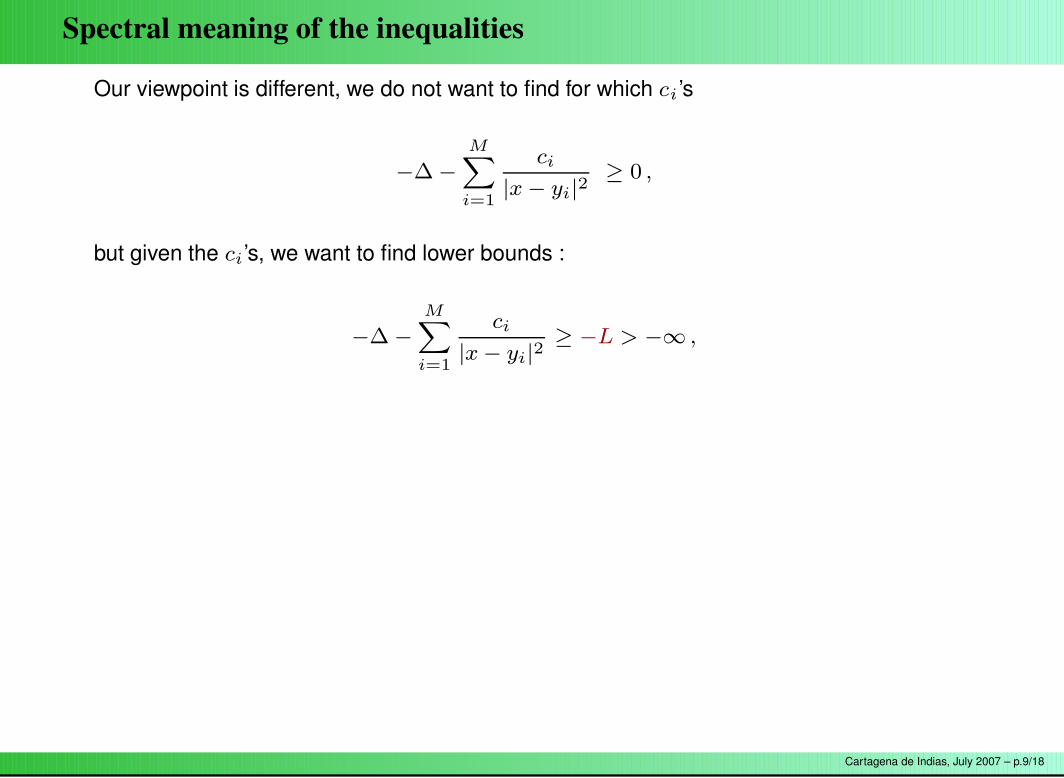
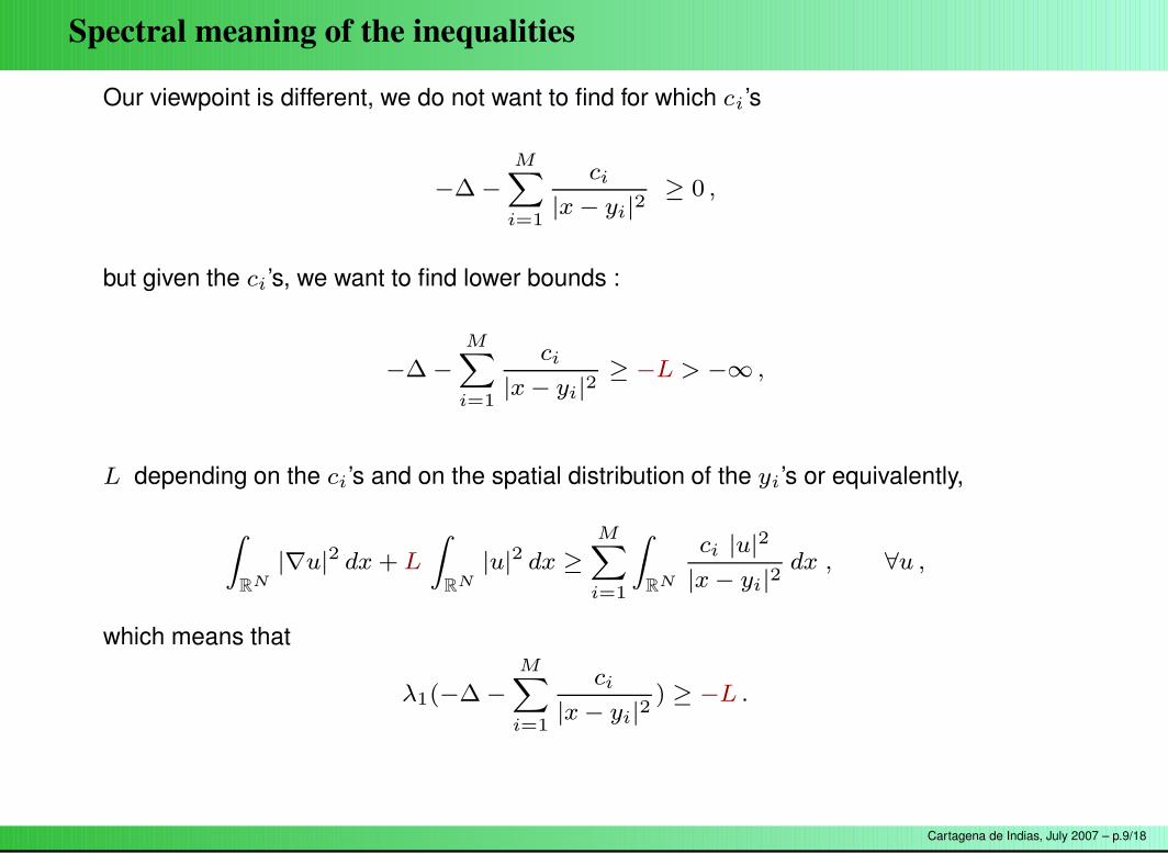
Our viewpoint is different, we do not want to find for which ci ’s
−∆ −MX
i=1
ci
|x − yi|2≥ 0 ,
but given the ci’s, we want to find lower bounds :
−∆ −MX
i=1
ci
|x − yi|2≥ −L > −∞ ,
L depending on the ci’s and on the spatial distribution of the yi’s or equivalently,
Z
RN
|∇u|2 dx + L
Z
RN
|u|2 dx ≥MX
i=1
Z
RN
ci |u|2
|x − yi|2dx , ∀u ,
which means that
λ1(−∆ −MX
i=1
ci
|x − yi|2) ≥ −L .
Cartagena de Indias, July 2007 – p.9/18
Spectral meaning of the inequalities
Our viewpoint is different, we do not want to find for which ci ’s
−∆ −MX
i=1
ci
|x − yi|2≥ 0 ,
but given the ci’s, we want to find lower bounds :
−∆ −MX
i=1
ci
|x − yi|2≥ −L > −∞ ,
L depending on the ci’s and on the spatial distribution of the yi’s or equivalently,
Z
RN
|∇u|2 dx + L
Z
RN
|u|2 dx ≥MX
i=1
Z
RN
ci |u|2
|x − yi|2dx , ∀u ,
which means that
λ1(−∆ −MX
i=1
ci
|x − yi|2) ≥ −L .
Cartagena de Indias, July 2007 – p.9/18

Why is this issue interesting?
1) In the study of crystalline matter.
2) In the study of stability of matter.
3) In general, in solid state physics problems, band gaps, etc.
But of course, only as an intermediate technical tool, since the problem we look atcorresponds to only 1 electron.
Cartagena de Indias, July 2007 – p.10/18
Scaling properties
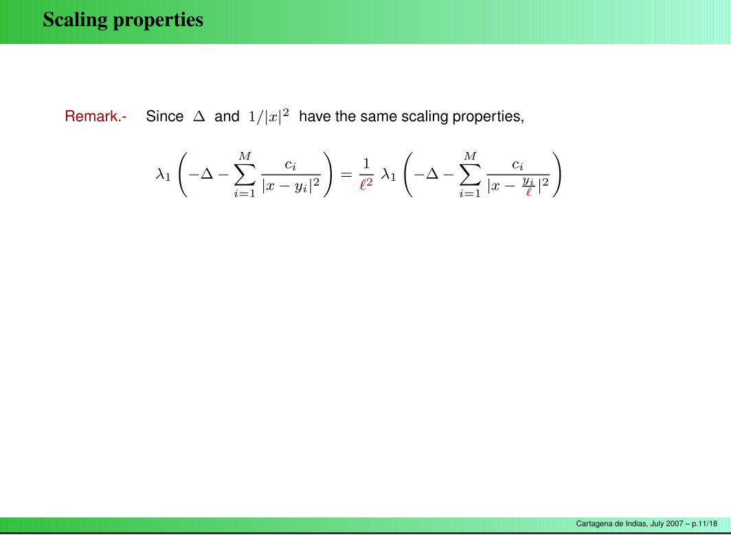
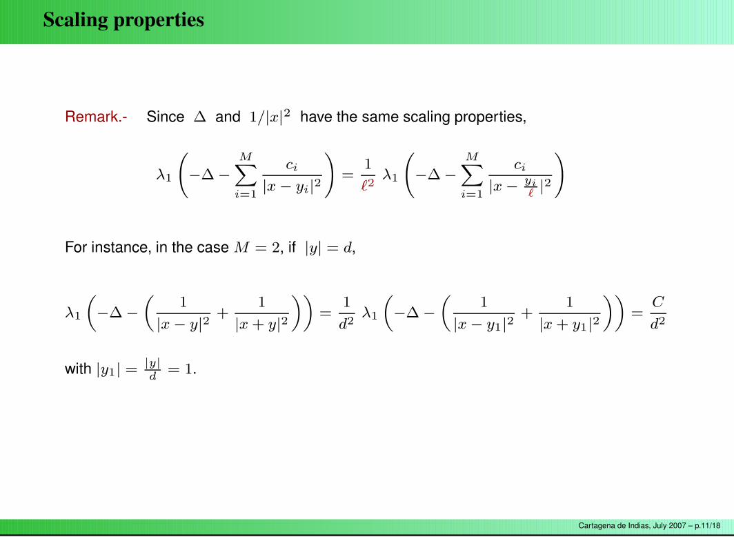
Remark.- Since ∆ and 1/|x|2 have the same scaling properties,
λ1
−∆ −MX
i=1
ci
|x − yi|2
!
=1
`2λ1
−∆ −MX
i=1
ci
|x − yi
`|2
!
For instance, in the case M = 2, if |y| = d,
λ1
„
−∆ −
„
1
|x − y|2+
1
|x + y|2
««
=1
d2λ1
„
−∆ −
„
1
|x − y1|2+
1
|x + y1|2
««
=C
d2
with |y1| =|y|d
= 1.
Cartagena de Indias, July 2007 – p.11/18
Scaling properties
Remark.- Since ∆ and 1/|x|2 have the same scaling properties,
λ1
−∆ −MX
i=1
ci
|x − yi|2
!
=1
`2λ1
−∆ −MX
i=1
ci
|x − yi
`|2
!
For instance, in the case M = 2, if |y| = d,
λ1
„
−∆ −
„
1
|x − y|2+
1
|x + y|2
««
=1
d2λ1
„
−∆ −
„
1
|x − y1|2+
1
|x + y1|2
««
=C
d2
with |y1| =|y|d
= 1.
Cartagena de Indias, July 2007 – p.11/18

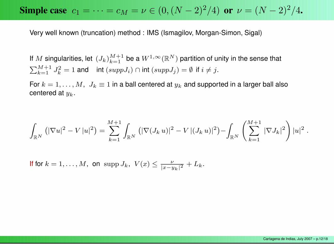
Simple case c1 = · · · = cM = ν ∈ (0, (N − 2)2/4) or ν = (N − 2)2/4.
Very well known (truncation) method : IMS (Ismagilov, Morgan-Simon, Sigal)
If M singularities, let (Jk)M+1k=1 be a W 1,∞(RN ) partition of unity in the sense that
PM+1k=1 J2
k = 1 and int (suppJi) ∩ int (suppJj) = ∅ if i 6= j.
For k = 1, . . . , M , Jk ≡ 1 in a ball centered at yk and supported in a larger ball alsocentered at yk .
Z
RN
`
|∇u|2 − V |u|2´
=
M+1X
k=1
Z
RN
`
|∇(Jk u)|2 − V |(Jk u)|2´
−
Z
RN
M+1X
k=1
|∇Jk|2
!
|u|2 .
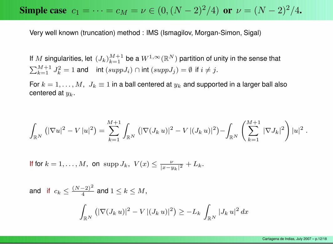
If for k = 1, . . . , M , on supp Jk, V (x) ≤ ν|x−yk|2
+ Lk.
and if ck ≤ (N−2)2
4and 1 ≤ k ≤ M ,
Z
RN
`
|∇(Jk u)|2 − V |(Jk u)|2´
≥ −Lk
Z
RN
|Jk u|2 dx
Cartagena de Indias, July 2007 – p.12/18

Simple case c1 = · · · = cM = ν ∈ (0, (N − 2)2/4) or ν = (N − 2)2/4.
Very well known (truncation) method : IMS (Ismagilov, Morgan-Simon, Sigal)
If M singularities, let (Jk)M+1k=1 be a W 1,∞(RN ) partition of unity in the sense that
PM+1k=1 J2
k = 1 and int (suppJi) ∩ int (suppJj) = ∅ if i 6= j.
For k = 1, . . . , M , Jk ≡ 1 in a ball centered at yk and supported in a larger ball alsocentered at yk .
Z
RN
`
|∇u|2 − V |u|2´
=
M+1X
k=1
Z
RN
`
|∇(Jk u)|2 − V |(Jk u)|2´
−
Z
RN
M+1X
k=1
|∇Jk|2
!
|u|2 .
If for k = 1, . . . , M , on supp Jk, V (x) ≤ ν|x−yk|2
+ Lk.
and if ck ≤ (N−2)2
4and 1 ≤ k ≤ M ,
Z
RN
`
|∇(Jk u)|2 − V |(Jk u)|2´
≥ −Lk
Z
RN
|Jk u|2 dx
Cartagena de Indias, July 2007 – p.12/18
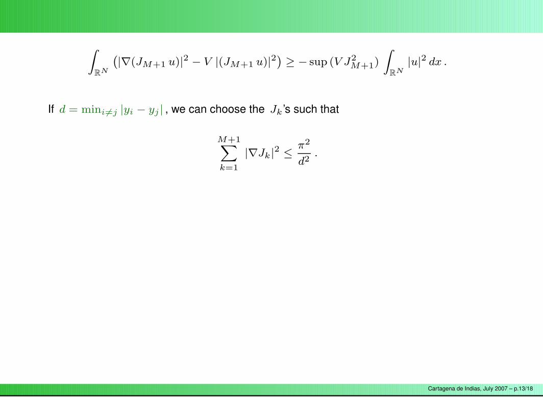
Z
RN
`
|∇(JM+1 u)|2 − V |(JM+1 u)|2´
≥ − sup (V J2M+1)
Z
RN
|u|2 dx .
If d = mini6=j |yi − yj | , we can choose the Jk ’s such that
M+1X
k=1
|∇Jk|2 ≤
π2
d2.
Finally, controlling the remainder a little bit more carefully than above, one obtains
Z
RN
|∇u|2 dx +“M ν
d2+
π2
d2
”
Z
RN
|u|2 dx ≥MX
i=1
Z
RN
ν |u|2
|x − yi|2dx ≥ 0 , ∀u ,
. . . and that implies that
λ1
“
− ∆ −MX
i=1
ν
|x − yi|2
”
≥ −M ν
d2−
π2
d2.
Cartagena de Indias, July 2007 – p.13/18

Z
RN
`
|∇(JM+1 u)|2 − V |(JM+1 u)|2´
≥ − sup (V J2M+1)
Z
RN
|u|2 dx .
If d = mini6=j |yi − yj | , we can choose the Jk ’s such that
M+1X
k=1
|∇Jk|2 ≤
π2
d2.
Finally, controlling the remainder a little bit more carefully than above, one obtains
Z
RN
|∇u|2 dx +“M ν
d2+
π2
d2
”
Z
RN
|u|2 dx ≥MX
i=1
Z
RN
ν |u|2
|x − yi|2dx ≥ 0 , ∀u ,
. . . and that implies that
λ1
“
− ∆ −MX
i=1
ν
|x − yi|2
”
≥ −M ν
d2−
π2
d2.
Cartagena de Indias, July 2007 – p.13/18
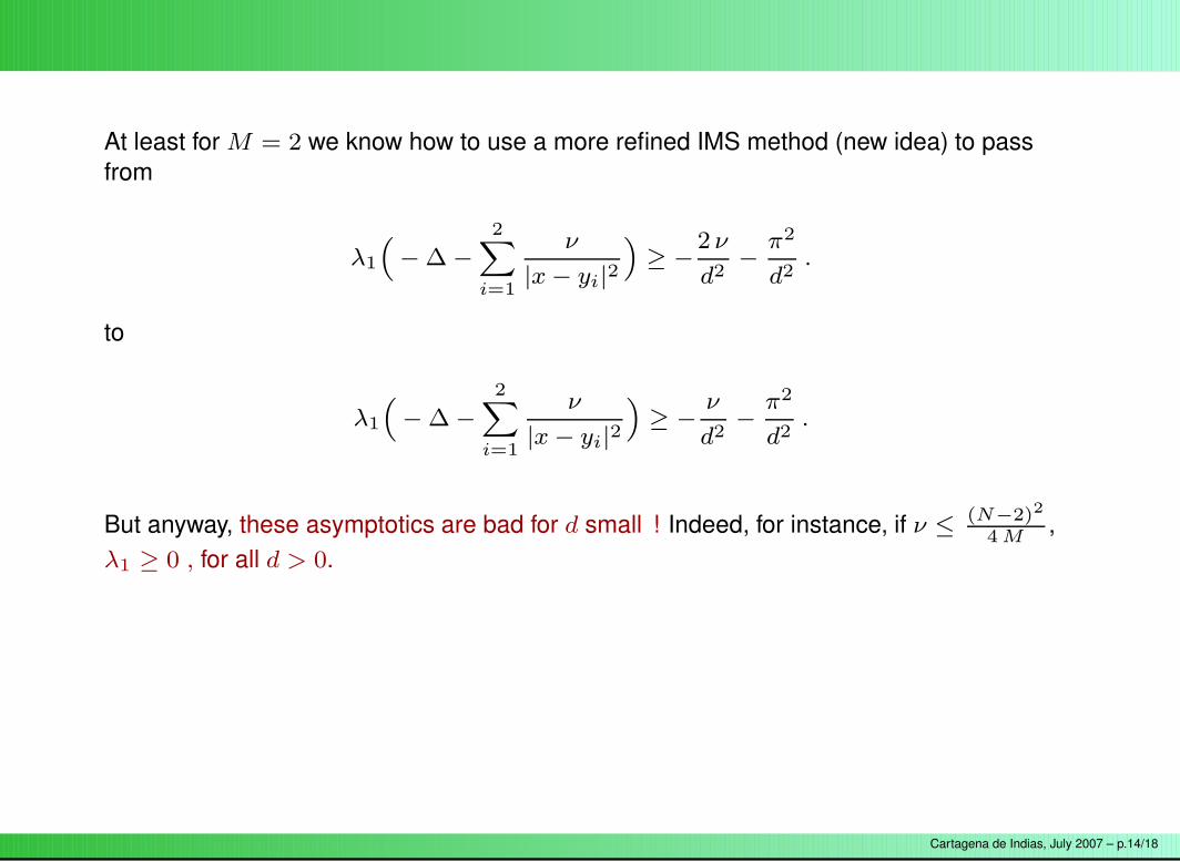
At least for M = 2 we know how to use a more refined IMS method (new idea) to passfrom
λ1
“
− ∆ −2X
i=1
ν
|x − yi|2
”
≥ −2 ν
d2−
π2
d2.
to
λ1
“
− ∆ −2X
i=1
ν
|x − yi|2
”
≥ −ν
d2−
π2
d2.
But anyway, these asymptotics are bad for d small ! Indeed, for instance, if ν ≤ (N−2)2
4 M,
λ1 ≥ 0 , for all d > 0.
Let us go back to the idea that Hardy inequalities can be obtained by expanding squares.
Cartagena de Indias, July 2007 – p.14/18
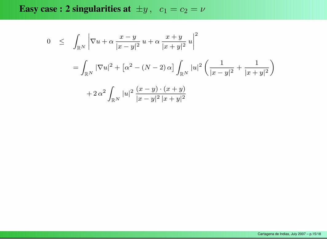
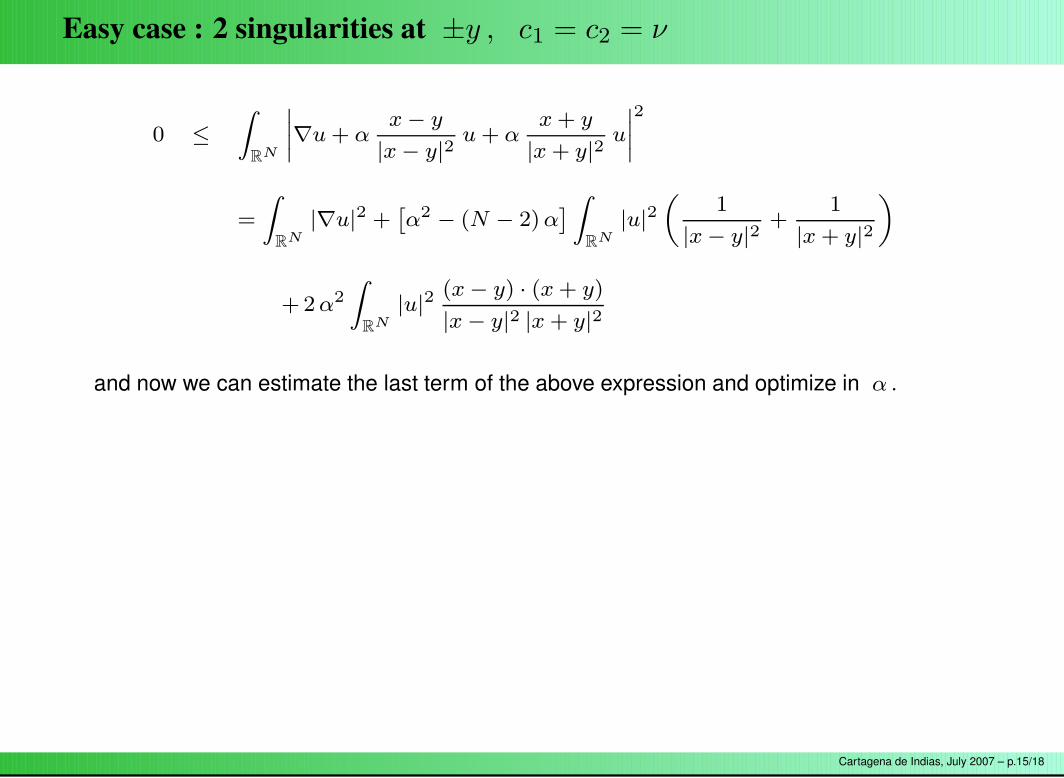
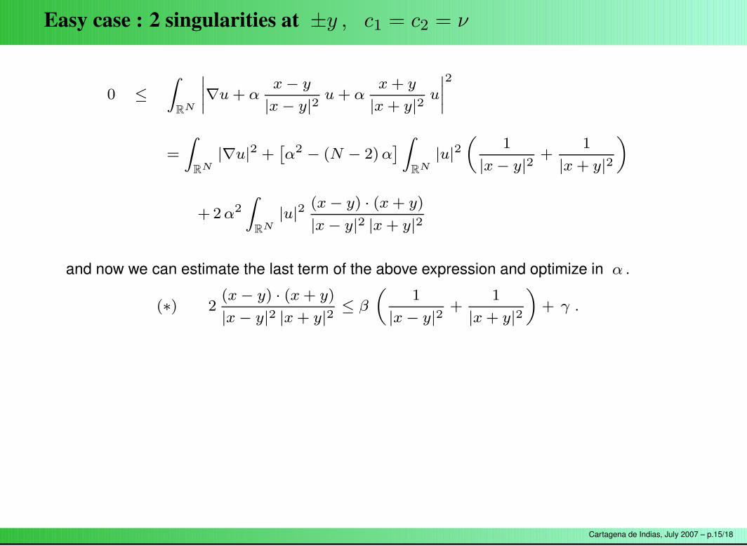
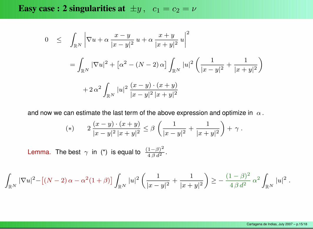
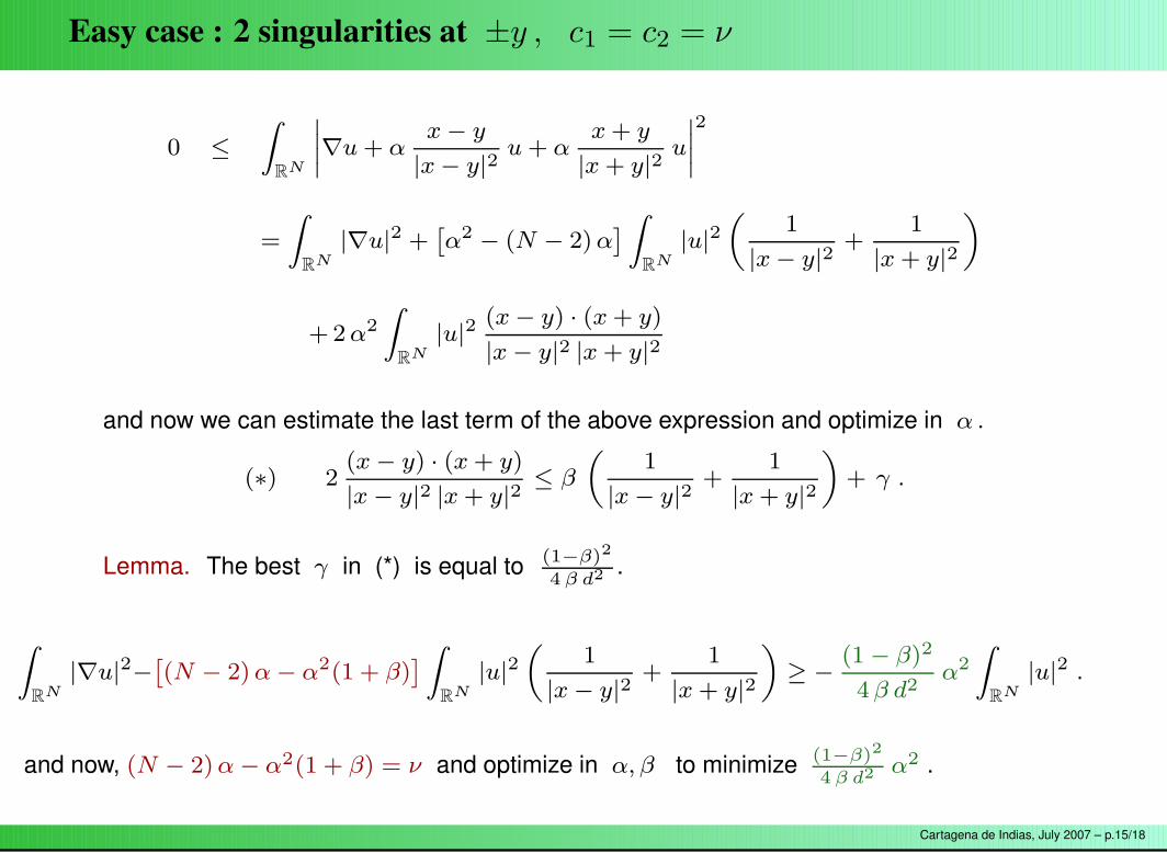
Easy case : 2 singularities at ±y , c1 = c2 = ν
0 ≤
Z
RN
˛
˛
˛
˛
∇u + αx − y
|x − y|2u + α
x + y
|x + y|2u
˛
˛
˛
˛
2
=
Z
RN
|∇u|2 +ˆ
α2 − (N − 2) α˜
Z
RN
|u|2„
1
|x − y|2+
1
|x + y|2
«
+2 α2
Z
RN
|u|2(x − y) · (x + y)
|x − y|2 |x + y|2
and now we can estimate the last term of the above expression and optimize in α .
(∗) 2(x − y) · (x + y)
|x − y|2 |x + y|2≤ β
„
1
|x − y|2+
1
|x + y|2
«
+ γ .
Lemma. The best γ in (*) is equal to (1−β)2
4 β d2 .
Z
RN
|∇u|2−ˆ
(N − 2) α − α2(1 + β)˜
Z
RN
|u|2„
1
|x − y|2+
1
|x + y|2
«
≥ −(1 − β)2
4 β d2α2
Z
RN
|u|2 .
and now, (N − 2) α − α2(1 + β) = ν and optimize in α, β to minimize (1−β)2
4 β d2 α2 .
Cartagena de Indias, July 2007 – p.15/18

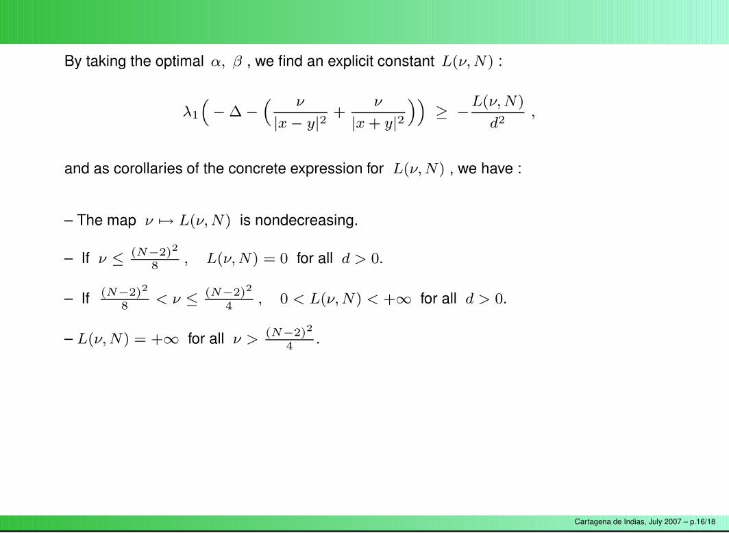
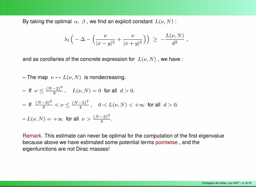
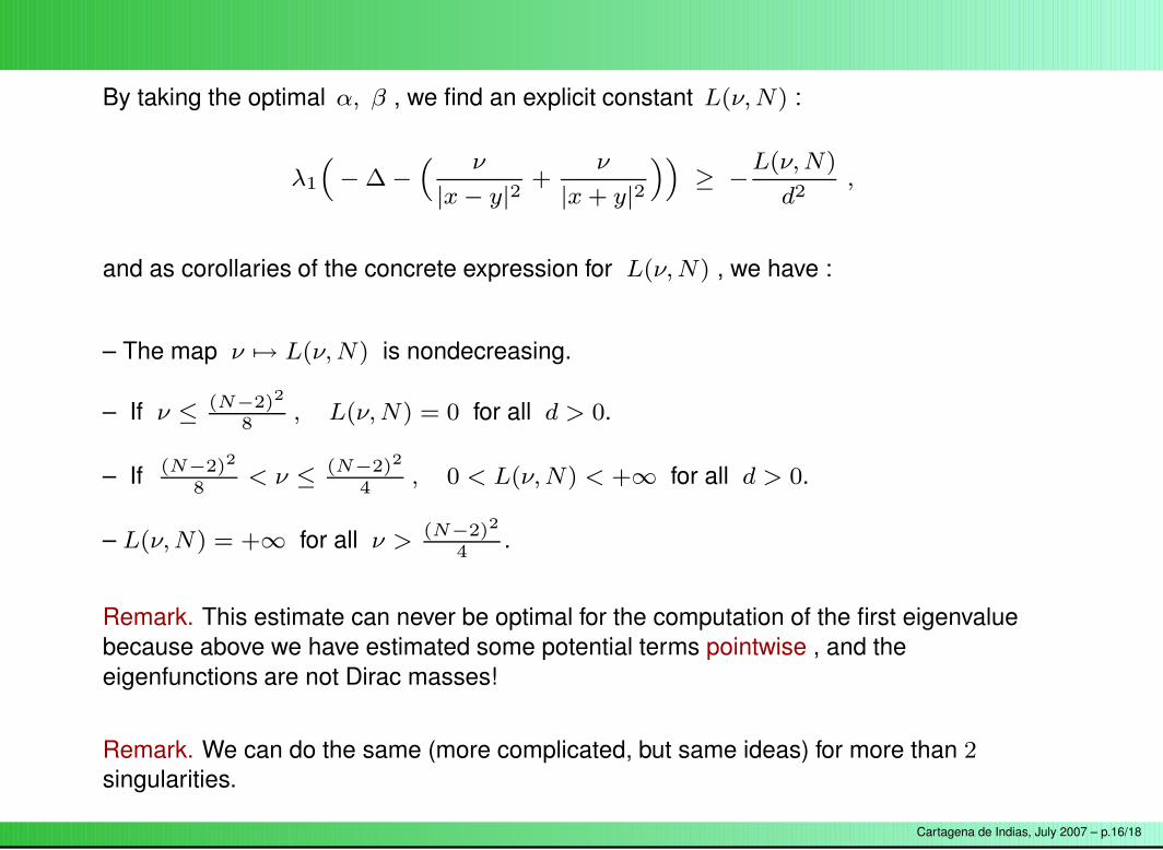
By taking the optimal α, β , we find an explicit constant L(ν, N) :
λ1
“
− ∆ −“ ν
|x − y|2+
ν
|x + y|2
””
≥ −L(ν, N)
d2,
and as corollaries of the concrete expression for L(ν, N) , we have :
– The map ν 7→ L(ν, N) is nondecreasing.
– If ν ≤ (N−2)2
8, L(ν, N) = 0 for all d > 0.
– If (N−2)2
8< ν ≤ (N−2)2
4, 0 < L(ν, N) < +∞ for all d > 0.
– L(ν, N) = +∞ for all ν >(N−2)2
4.
Remark. This estimate can never be optimal for the computation of the first eigenvaluebecause above we have estimated some potential terms pointwise , and theeigenfunctions are not Dirac masses!
Remark. We can do the same (more complicated, but same ideas) for more than 2singularities.
Cartagena de Indias, July 2007 – p.16/18

Comparison between the two methods
IMS, which is the method traditionally used in this kind of business, is good for distantsingularities, but the square expanding method gives much better estimates for nearbysingularities.
In a recent work Javier Duoandikoetxea and Luis Vega have explored a new(geometrical) method to compute the lowest eigenvalues of −∆ − V in R
N for anonnegative potential V in MN/2(RN ) with only one singularity.
Even more recently, we have extended it to the Dirac case together with Jean Dolbeault,Javier Duoandikoetxea and Luis Vega.
Right now we are working on the extension of this new method to the case of severalsingularities, and we are optimistic about getting much better estimates for d small thanwith the other 2 methods. To follow...
Cartagena de Indias, July 2007 – p.17/18

Same kind of things can be done for other operators... like the Dirac operator (first orderand unbounded from below !).
THE END
Cartagena de Indias, July 2007 – p.18/18

Same kind of things can be done for other operators... like the Dirac operator (first orderand unbounded from below !).
THE END
Cartagena de Indias, July 2007 – p.18/18