
Hamilton-Jacobi-Bellman Equation of an Optimal Consumption ...shuenn-jyi.pdf ·...
61
Hamilton-Jacobi-Bellman Equation of an Optimal Consumption Problem Shuenn-Jyi Sheu Institute of Mathematics, Academia Sinica WSAF, CityU HK June 29-July 3, 2009
Transcript of Hamilton-Jacobi-Bellman Equation of an Optimal Consumption ...shuenn-jyi.pdf ·...
Hamilton-Jacobi-Bellman Equation of anOptimal Consumption Problem
Shuenn-Jyi Sheu
Institute of Mathematics, Academia Sinica
WSAF, CityU HK
June 29-July 3, 2009
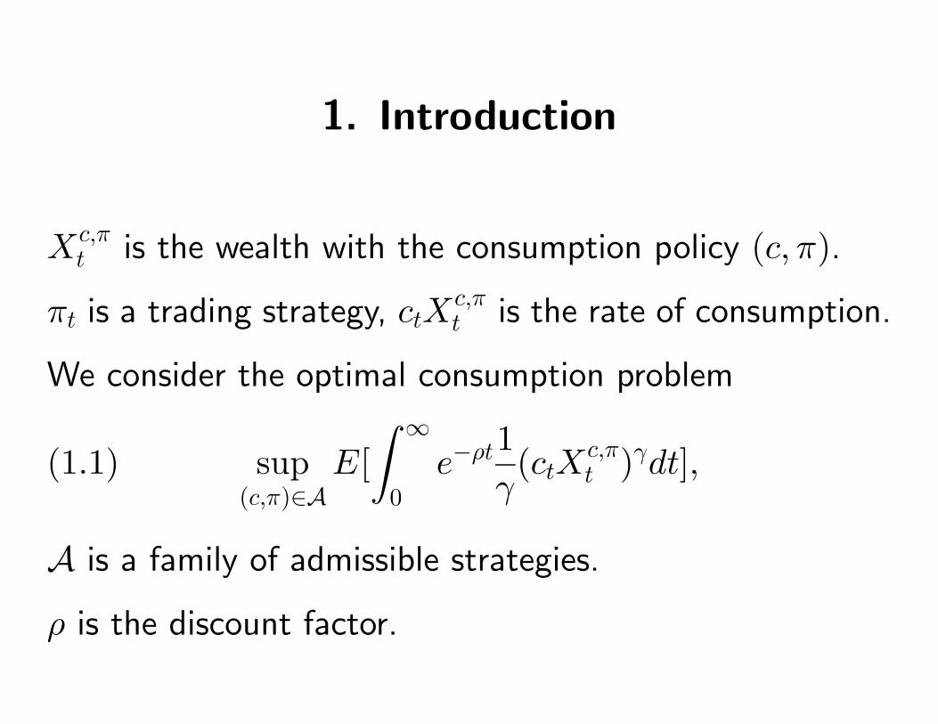
1. Introduction
Xc,πt is the wealth with the consumption policy (c, π).
πt is a trading strategy, ctXc,πt is the rate of consumption.
We consider the optimal consumption problem
(1.1) sup(c,π)∈A
E[∫ ∞
0e−ρt
1γ(ctX
c,πt )γdt],
A is a family of admissible strategies.
ρ is the discount factor.
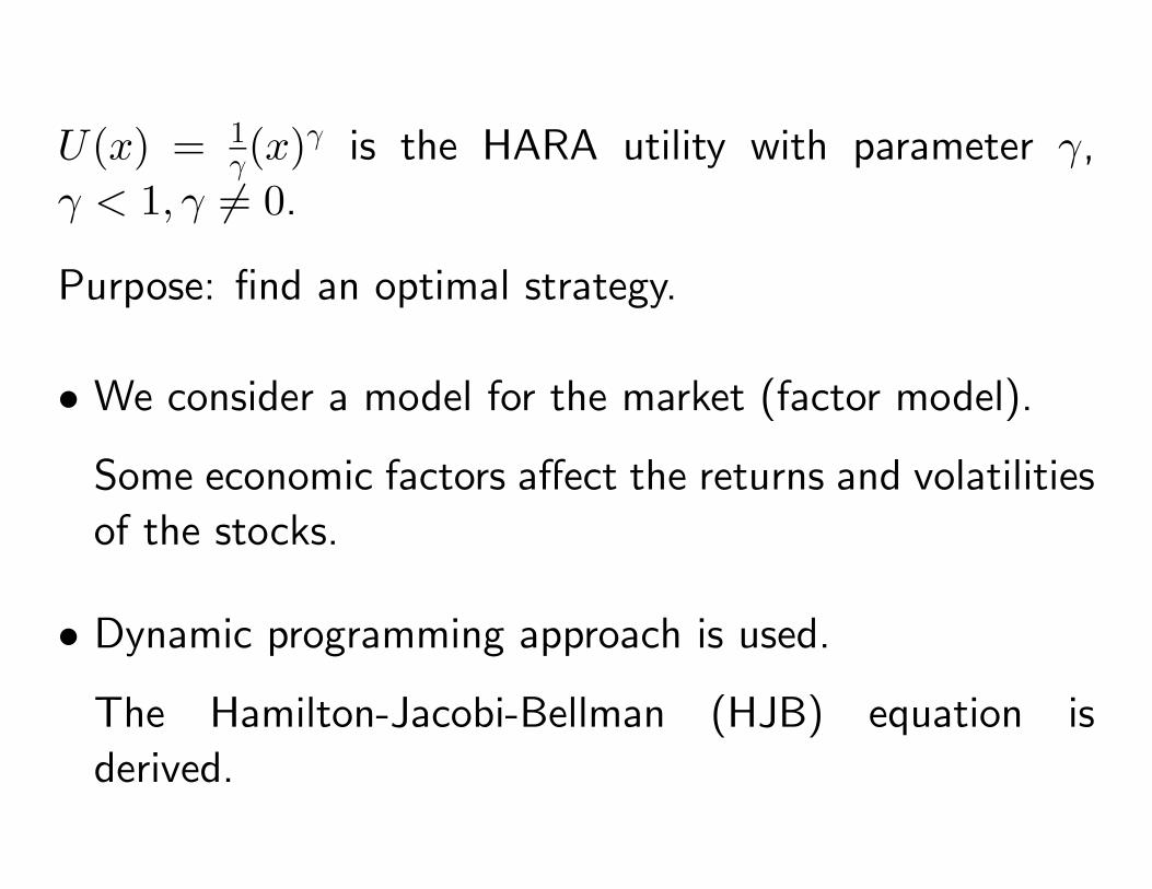
U(x) = 1γ(x)
γ is the HARA utility with parameter γ,
γ < 1, γ 6= 0.
Purpose: find an optimal strategy.
• We consider a model for the market (factor model).
Some economic factors affect the returns and volatilities
of the stocks.
• Dynamic programming approach is used.
The Hamilton-Jacobi-Bellman (HJB) equation is
derived.
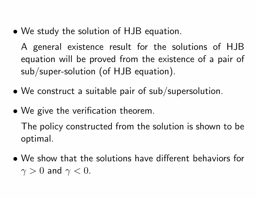
• We study the solution of HJB equation.
A general existence result for the solutions of HJB
equation will be proved from the existence of a pair of
sub/super-solution (of HJB equation).
• We construct a suitable pair of sub/supersolution.
• We give the verification theorem.
The policy constructed from the solution is shown to be
optimal.
• We show that the solutions have different behaviors for
γ > 0 and γ < 0.
References
H.Hata and S.J.Sheu (2009), Hamilton-Jacobi-Bellman
equation for an optimal consumption problem, preprint.
H.Hata and S.J.Sheu (2009), An optimal consumption
and investment problem with linear Gaussian model,
preprint.
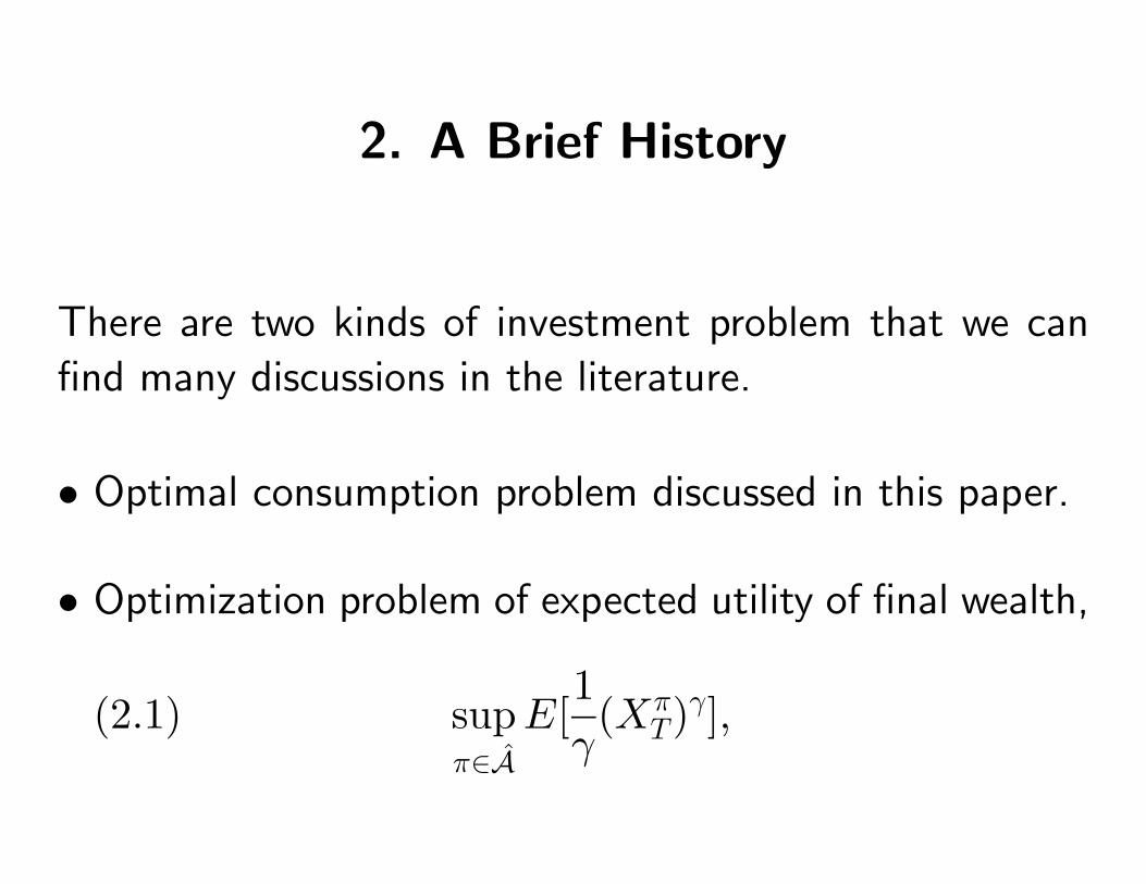
2. A Brief History
There are two kinds of investment problem that we can
find many discussions in the literature.
• Optimal consumption problem discussed in this paper.
• Optimization problem of expected utility of final wealth,
(2.1) supπ∈A
E[1γ(Xπ
T)γ],
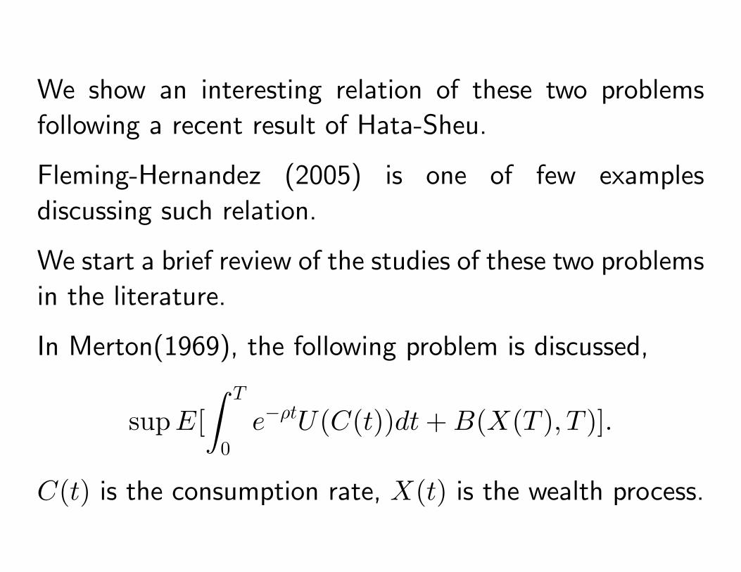
We show an interesting relation of these two problems
following a recent result of Hata-Sheu.
Fleming-Hernandez (2005) is one of few examples
discussing such relation.
We start a brief review of the studies of these two problems
in the literature.
In Merton(1969), the following problem is discussed,
supE[∫ T
0e−ρtU(C(t))dt+B(X(T ), T )].
C(t) is the consumption rate, X(t) is the wealth process.
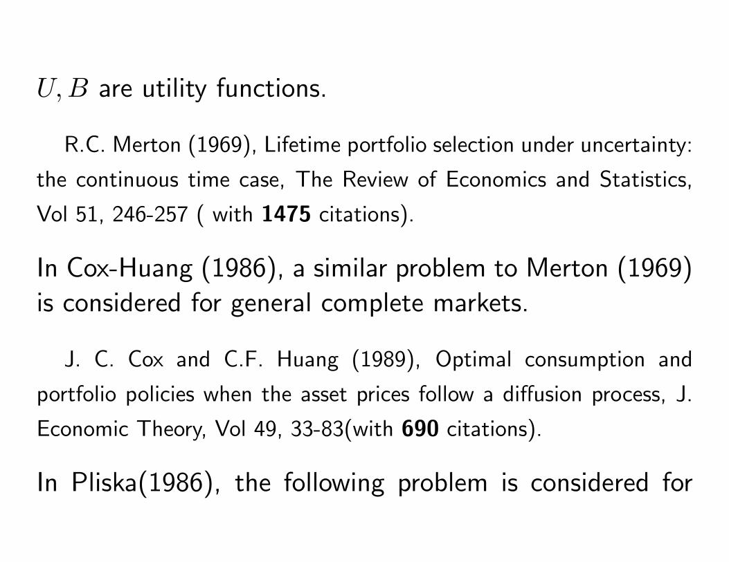
U,B are utility functions.
R.C. Merton (1969), Lifetime portfolio selection under uncertainty:
the continuous time case, The Review of Economics and Statistics,
Vol 51, 246-257 ( with 1475 citations).
In Cox-Huang (1986), a similar problem to Merton (1969)
is considered for general complete markets.
J. C. Cox and C.F. Huang (1989), Optimal consumption and
portfolio policies when the asset prices follow a diffusion process, J.
Economic Theory, Vol 49, 33-83(with 690 citations).
In Pliska(1986), the following problem is considered for
the complete market with general diffusion model,
supπE[U(Xπ(T ))].
S. Pliska(1986), A stochastic calculus model of continuous trading:
optimal portfolios, Math. Operation Research Vol.11, 371-382 (with
218 citations)
The developments in Pliska(1986) and Cox-Huang
(1989) start the use of stochastic calculus, martingale
representation theorem and duality argument.
Using their approach, the optimal solution can be explicitly
calculated without solving PDE.
This is very interesting and is also a reason for receiving
so many citations.
Their method is different from the approach in Merton
(1969).
In Merton (1969), the solution is obtained by solving the
HJB (Hamilton-Jacobi-Bellman) equation. HJB is a PDE
(partial differential equation). For a simple model, the
equation can be solved explicitly. In general, it is difficult
to calculate the solution.
The idea in Pliska, Cox-Huang can not be applied to
incomplete markets.
Previous studies have suggested some possible directions
for research:
• Obtain an explicit solution by generalizing the idea of
Pliska and Cox-Huang.
• Study HJB equation.
In practice, it is also important to solve the equation
numerically, if an analytical solution is not possible.
In addition to these, there are also a huge number
of possible applications can suggest many interesting
problems.
The following show some models which have analytical
solution, Wachter(2002),Chacko-Viceira(2005),Jun Liu
(2007)
An initial attempt to use HJB equation in more
complicated models is first proposed in Fleming (1995).
The idea is to reformulate the investment problem
as a stochastic control problem. Then the dynamic
programming approach can be used to derive the HJB
equation. Solving HJB equation will provide a candidate
of optimal investment strategy.
This suggests several interesting questions for the solutions
of such HJB equations.
• Study the regularity, growth conditions of the solutions.
• Obtain suitable estimates for the solutions.
This is needed when we want to prove the candidate
of optimal portfolio derived from a solution is indeed
optimal (verification theorem).
To show how this works, Fleming-Sheu(1999) study a
simple model different from that of Merton(1969) and
provides a detailed analysis.
The model can be briefly described as follows
There is one stock and one banking account that an
investor can trade.
The interest rate for the banking account is constant
r > 0.
The price of stock is given by
Pt = exp(Lt),
dLt = c(µt+ α0 − Lt)dt+ σdWt.
It turns out that the model in Fleming-Sheu (1999), after
reformulation, becomes a special case of factor model.
y(t) = Lt − µt− (α0 −µ
c)
plays the role of factor.
Using this approach, the risk-sensitive portfolio
optimization problem for more general factor models have
been considered in a list of papers:
Fleming-Sheu (1999a, b), Fleming-Sheu(2002),
Kuroda-Nagai(2002), Nagai-Peng(2002), Nagai(2003),
Kaise-Sheu(2004), Hata-Sekine(2005), Bilecki-Pliska-
Sheu(2005)
An useful theorem about the structure of the solutions of
HJB equation is given in Kaise-Sheu(2006).
The studies mentioned above have interesting applications
to the minimization of down-side risk probabilities,
(2.2) minP (logXπ
T
T≤ k).
There is a duality relation between (2.2) and the risk
sensitive portfolio optimization problem (2.1) with a
particular risk sensitive parameter γ = γ(k) < 0.
The following is a list of papers,
Hata-Nagai-Sheu(2009), Hata-Sheu(2008), Hata(2008),
Nagai(2008, 2009)
The result is interesting because of the following reasons.
• The problem (2.2) is not a conventional optimization
problem and a direct solution is not available.
The result shows that we can solve (2.2) using a solution
of (2.1).
• HARA utility appears naturally from (2.2). Although
(2.2) seems to not have relation with utilty function at
the first look.
For this connection, see also works of Pham (2003) on
the maximization problem of up-side chance probabilities,
maxP (logXπ
T
T≥ c).
We remark that a recent work of Follmer-Schachermayer
(2008) seems to also relate to our study,
In this talk, we will discuss another application of the
study of the risk sensitive portfolio optimization problem
(2.1) to the consumption problem in (1.1).
This application seems to not be expected from the results
in the literature.
We are motivated by the three recent papers, Fleming-
Hernandez(2003, 2005), Fleming-Pang(2004).
Fleming-Pang (2004) considers a model that the stock
price is geometric Brownian motion and interest rate of
the banking account is random and is an ergodic 1-d
diffusion process.
We also use an approach similar to Fleming-Pang (2004).
We show that a solution of HJB for (2.1) can be used to
construct a supersolution for the HJB of (1.1). Then a
nice solution of the HJB for (1.1) can be obtained. From
this, (1.1) can be solved.
We develop some useful ideas for general factor models
with multiple stocks.
An attempt to use the duality argument similar to
that in Pliska(1986)and Cox-Huang(1989) is proposed
in Castaneda-Hernandez (2005)for general factor models.
A solution is given in the case of HARA utility. However,
the result for general utilities is not satisfactory.
References
Analytical Solution
• J.A. Wachter(2002), Portfolio and consumption decisions under
mean-reverting ruturns: an exact solution for complete markets, J.
Financ. Quant. Anal. 37, 63-91.
• Chacko, G. and Viceira, L.M.(2005), Dynamic consumption and
portfolio choice with stochastic volatility in incomplete markets,
Rev. Financ. Stud. 18, 1369-1402.
• Jun Liu (2007), Portfolio selection in stochastic enviroments, Rev.
Financ. Stud. 20, 1-39.
Risk Sensitive Portfolio Optimization
• Fleming, W.H.(1995),Optimal investment models and risk-sensitive
stochastic control. Mathematical Finance (Davis M, et al,ed),
Spring-Verlag, Berlin.
• W.H. Fleming and S. J. Sheu (1999), optimal long term growth
rate of expected utility of wealth, Ann. Appl. Probab., Vol 9,
871-903
• W.H. Fleming and S.J. Sheu (1999), Risk sensitive control and an
optimal investment model, Math. Finance 10, 197-213.
• W.H. Fleming and S.J. Sheu (2002), Risk sensitive control and an
optimal investment model II, Ann. Appl. Probab. 12, 730-767.
• K. Kuroda and H. Nagai (2002), risk sensitive portfolio optimization
on infinite time horizon, Stoch. Stoch. Report, 73, 309-331
• H. Nagai and S. Peng (2002), Risk sensitive portfolio optimization
with partial information on infinite time horizon, Ann. Appl.
Probab. 12, 173-195.
• H. Nagai (2003), Optimal strategies for risk-sensitive portfolio
optimization problems for general models, SIAM J. Cont. Optim.
41, 1779-1800.
• H. Kaise and S.J. Sheu (2004), Risk sensitive optimal investment:
solutions of the dynamical programming equation. In Mathematics
of Finance, Contemp. Math. 351, 217-230.
• H. Hata and J. Sekine (2005), Solving long term optimal
investment problems with Cox-Ingersol-Ross interest rates, Advance
in Mathematical Economics 8, 231-255.
• T.R. Bielecki, S. Pliska and S.J. Sheu (2005), Risk-sensitive
portfolio management with Cox-Ingersol-Ross interest rates:HJB
equation, SIAM J. Cont. Optim. 44, 1811-1843.
• H. Kaise and S. J. Sheu (2006), On the structure of solutions of
ergodic type Bellman equations related to risk-sensitive control,
Ann. Probab. 34, 284-320.
Down-side Risk probability
• H. Hata, H. Nagai and S.J. Sheu (2009), Asymptotics of probability
minimizing a down-side risk, to appear in Ann. Appl. Probab.
• H. Hata and S.J. Sheu (2008), Down-side risk probability
minimization problem for a multidimensional model with stochastic
volatility, preprint.
• H. Hata (2008), Down-side risk large deviations control problem
with Cox-Ingersoll-Ross interest rates, preprint.
• H. Nagai (2008), Asymptotics of the probability minimizing a
”down-side” risk under partial information, preprint.
• H. Nagai (2009), Down-side risk minimization as large deviation
control, preprint.
• H. Follmer and W. Schachermayer (2008), Asymptotic arbitrage
and large deviations, preprint.
Optimal Consumption
• W.H. Fleming and D. Hernandez-Hernandez (2003), An optimal
consumption model with stochastic volatility, Finance Stochastics,
7, 245-262.
• W.H. Fleming and T. Pang (2004), An application of stochastic
control theory to financial economics, SIAM J. Control Optim., 43,
502-531
• W.H. Fleming and D. Hernandez-Hernandez (2005), The tradeoff
between consumption and investment in incomplete markets, Appl.
Math. Optim., 52, 219-235.
• N. Castaneda, D. Hernandez-Hernandez (2005), Optimal
consumption-investment problems in incomplete markets with
stochastic coefficients, SIAM J. Cont. Optim., 44, 1322-1344.
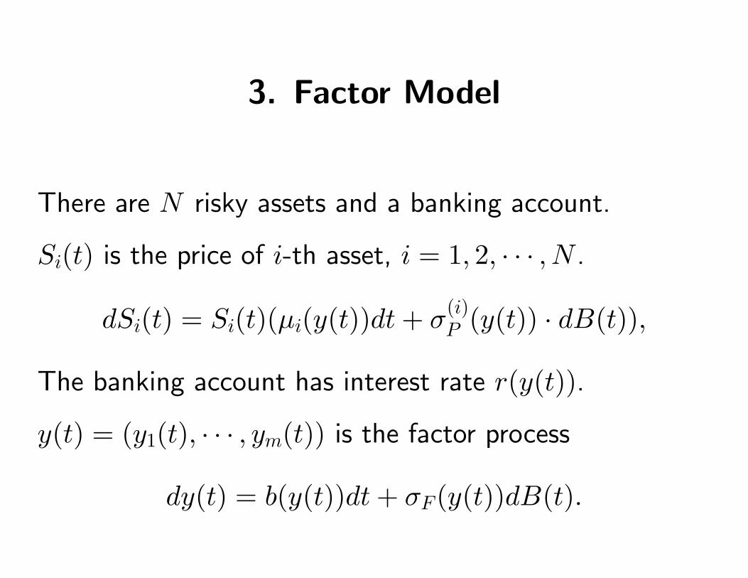
3. Factor Model
There are N risky assets and a banking account.
Si(t) is the price of i-th asset, i = 1, 2, · · · , N .
dSi(t) = Si(t)(µi(y(t))dt+ σ(i)P (y(t)) · dB(t)),
The banking account has interest rate r(y(t)).
y(t) = (y1(t), · · · , ym(t)) is the factor process
dy(t) = b(y(t))dt+ σF(y(t))dB(t).
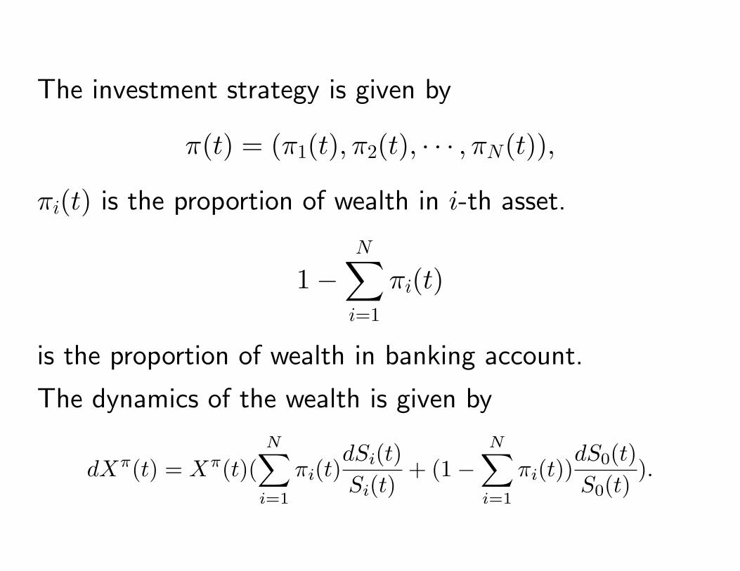
The investment strategy is given by
π(t) = (π1(t), π2(t), · · · , πN(t)),
πi(t) is the proportion of wealth in i-th asset.
1−N∑i=1
πi(t)
is the proportion of wealth in banking account.
The dynamics of the wealth is given by
dXπ(t) = Xπ(t)(N∑
i=1
πi(t)dSi(t)Si(t)
+ (1−N∑
i=1
πi(t))dS0(t)S0(t)
).
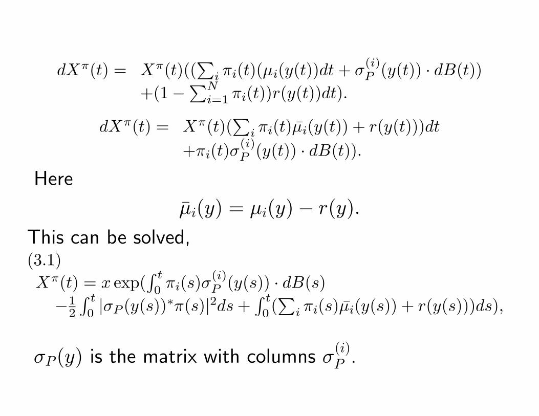
dXπ(t) = Xπ(t)((∑
i πi(t)(µi(y(t))dt+ σ(i)P (y(t)) · dB(t))
+(1−∑N
i=1 πi(t))r(y(t))dt).
dXπ(t) = Xπ(t)(∑
i πi(t)µi(y(t)) + r(y(t)))dt+πi(t)σ
(i)P (y(t)) · dB(t)).
Here
µi(y) = µi(y)− r(y).This can be solved,(3.1)Xπ(t) = x exp(
∫ t
0πi(s)σ
(i)P (y(s)) · dB(s)
−12
∫ t
0|σP (y(s))∗π(s)|2ds+
∫ t
0(∑
i πi(s)µi(y(s)) + r(y(s)))ds),
σP(y) is the matrix with columns σ(i)P .
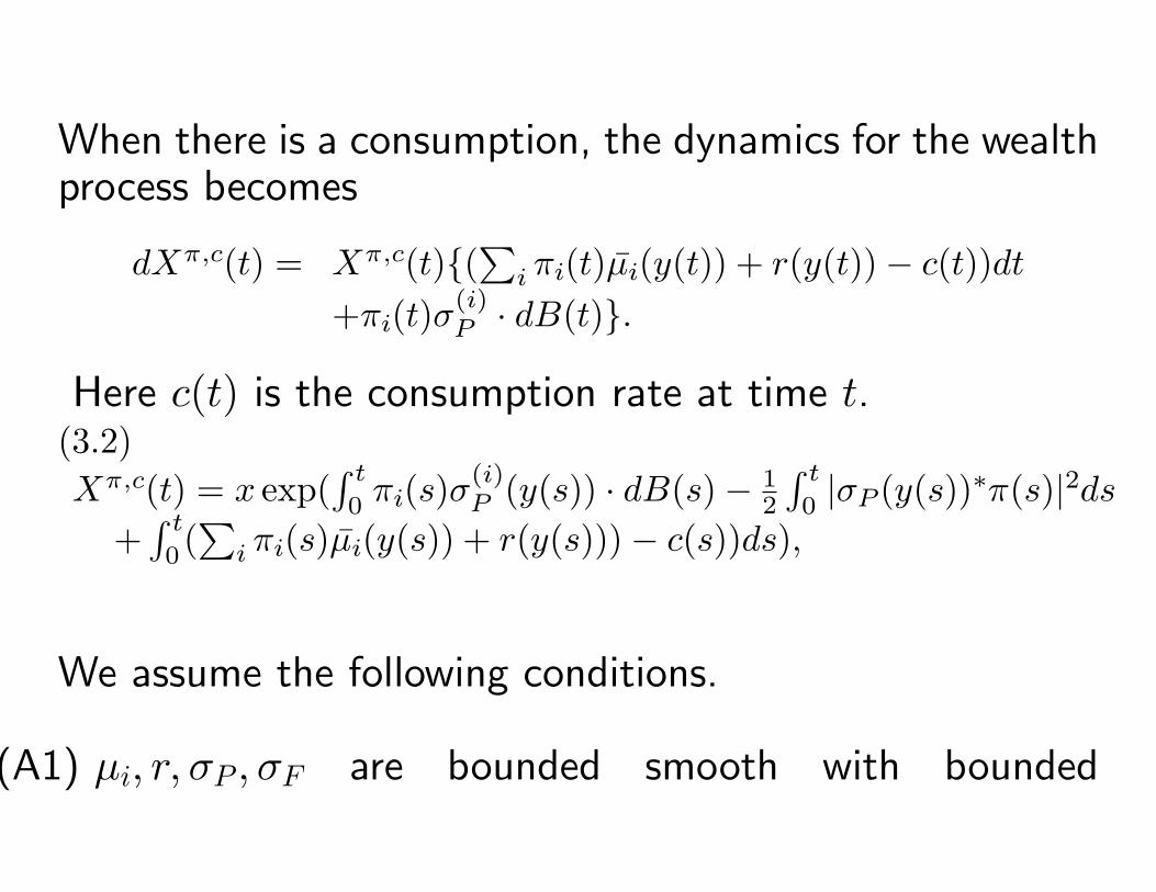
When there is a consumption, the dynamics for the wealthprocess becomes
dXπ,c(t) = Xπ,c(t){(∑
i πi(t)µi(y(t)) + r(y(t))− c(t))dt+πi(t)σ
(i)P · dB(t)}.
Here c(t) is the consumption rate at time t.(3.2)Xπ,c(t) = x exp(
∫ t
0πi(s)σ
(i)P (y(s)) · dB(s)− 1
2
∫ t
0|σP (y(s))∗π(s)|2ds
+∫ t
0(∑
i πi(s)µi(y(s)) + r(y(s)))− c(s))ds),
We assume the following conditions.
(A1) µi, r, σP , σF are bounded smooth with bounded
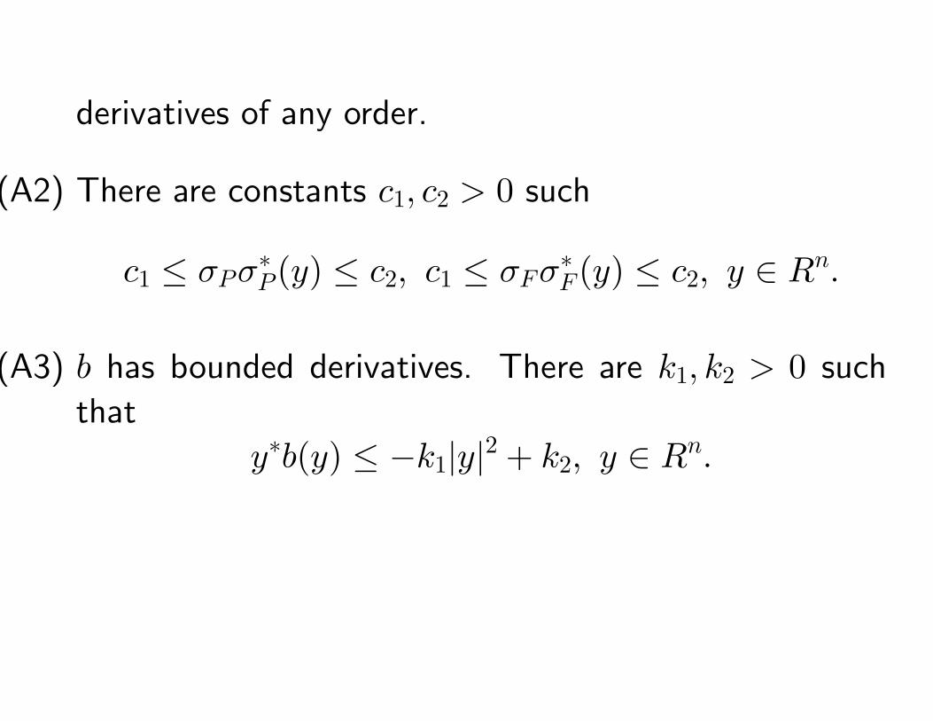
derivatives of any order.
(A2) There are constants c1, c2 > 0 such
c1 ≤ σPσ∗P(y) ≤ c2, c1 ≤ σFσ
∗F(y) ≤ c2, y ∈ Rn.
(A3) b has bounded derivatives. There are k1, k2 > 0 such
that
y∗b(y) ≤ −k1|y|2 + k2, y ∈ Rn.
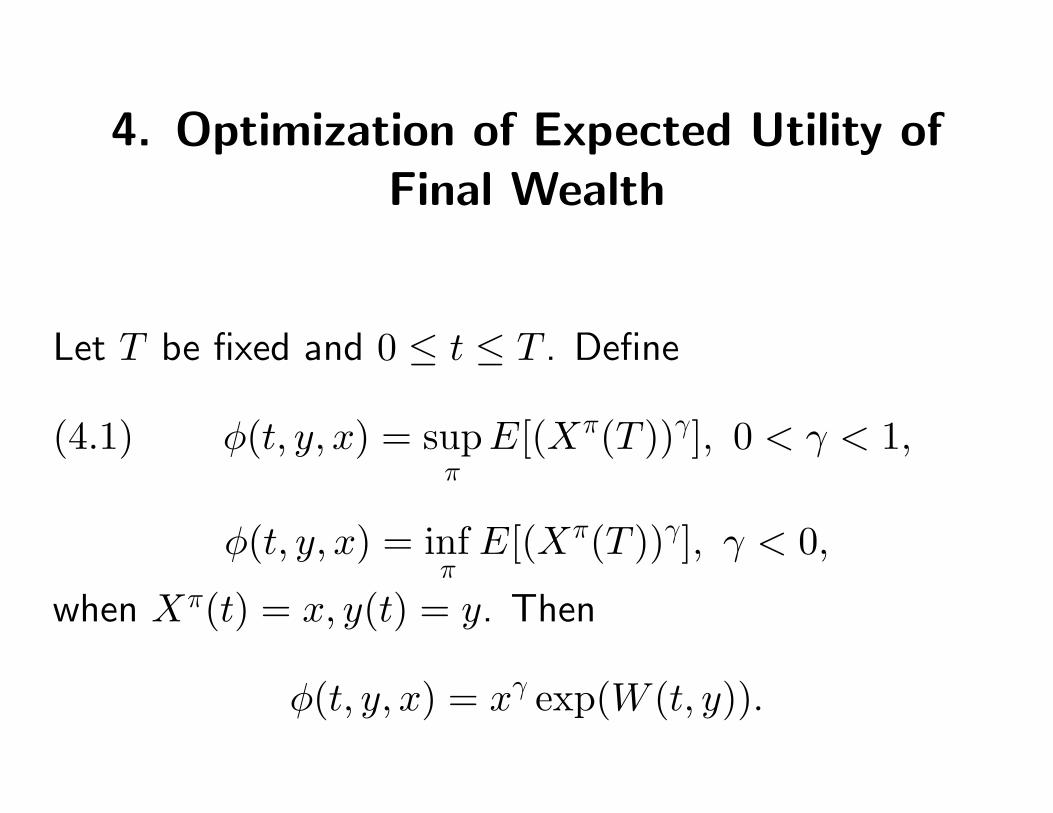
4. Optimization of Expected Utility ofFinal Wealth
Let T be fixed and 0 ≤ t ≤ T . Define
(4.1) φ(t, y, x) = supπE[(Xπ(T ))γ], 0 < γ < 1,
φ(t, y, x) = infπE[(Xπ(T ))γ], γ < 0,
when Xπ(t) = x, y(t) = y. Then
φ(t, y, x) = xγ exp(W (t, y)).
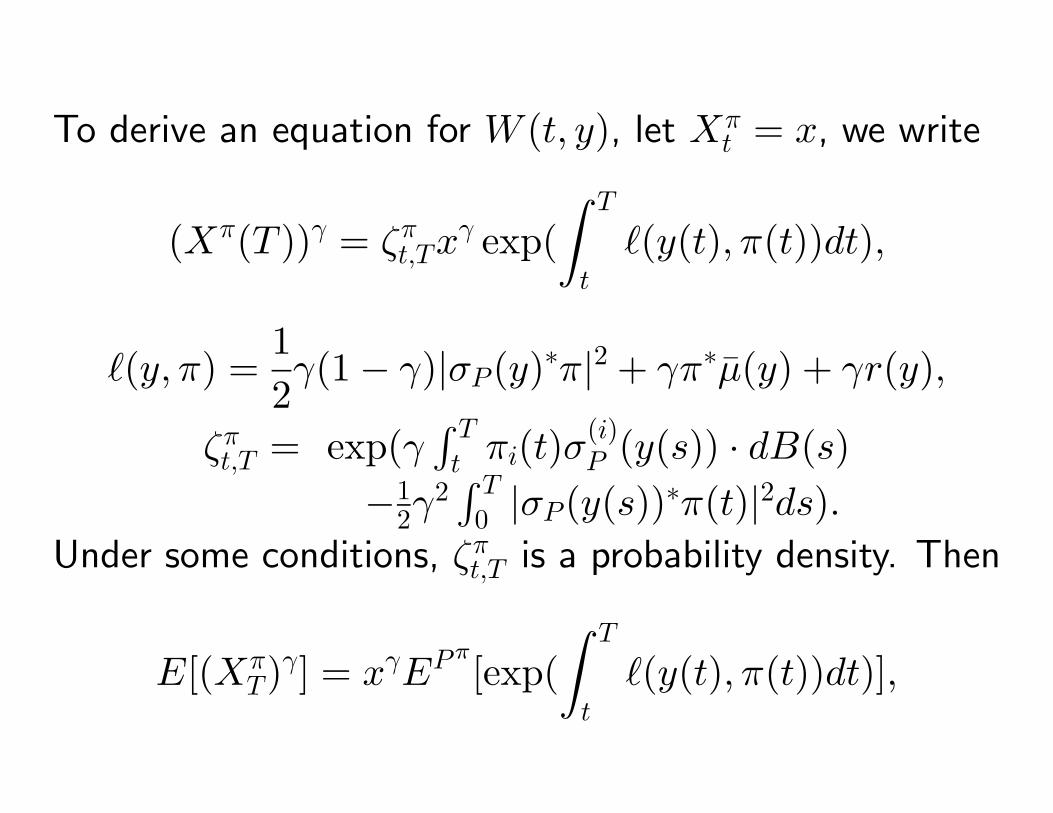
To derive an equation for W (t, y), let Xπt = x, we write
(Xπ(T ))γ = ζπt,Txγ exp(
∫ T
t
`(y(t), π(t))dt),
`(y, π) =12γ(1− γ)|σP(y)∗π|2 + γπ∗µ(y) + γr(y),
ζπt,T = exp(γ∫ T
t πi(t)σ(i)P (y(s)) · dB(s)
−12γ
2∫ T
0 |σP(y(s))∗π(t)|2ds).Under some conditions, ζπt,T is a probability density. Then
E[(XπT)
γ] = xγEPπ[exp(
∫ T
t
`(y(t), π(t))dt)],
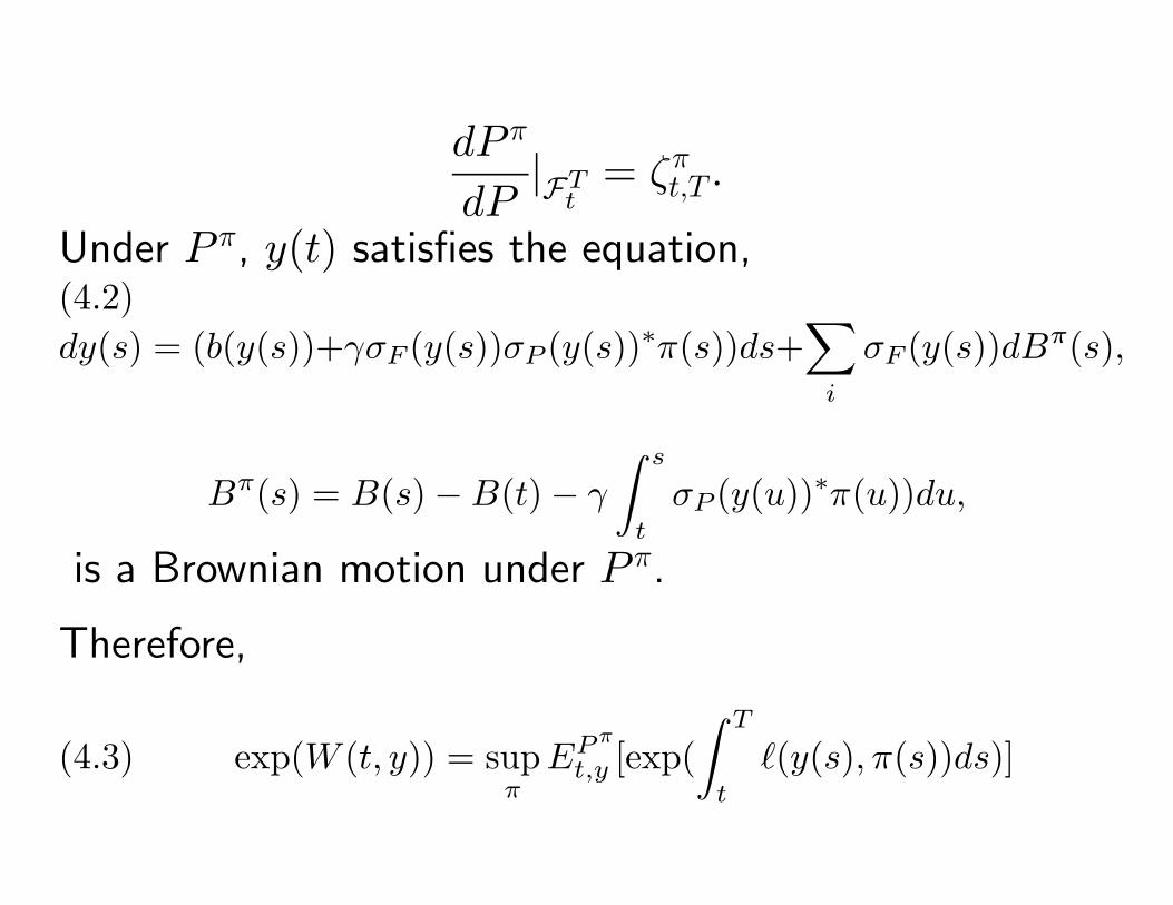
dP π
dP|FT
t= ζπt,T .
Under P π, y(t) satisfies the equation,(4.2)dy(s) = (b(y(s))+γσF (y(s))σP (y(s))∗π(s))ds+
∑i
σF (y(s))dBπ(s),
Bπ(s) = B(s)−B(t)− γ
∫ s
t
σP (y(u))∗π(u))du,
is a Brownian motion under P π.
Therefore,
(4.3) exp(W (t, y)) = supπEP π
t,y [exp(∫ T
t
`(y(s), π(s))ds)]
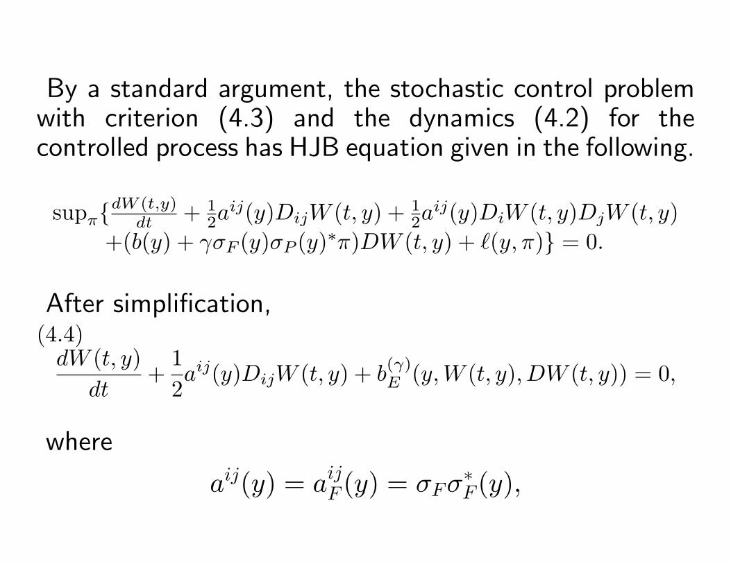
By a standard argument, the stochastic control problemwith criterion (4.3) and the dynamics (4.2) for thecontrolled process has HJB equation given in the following.
supπ{dW (t,y)
dt + 12a
ij(y)DijW (t, y) + 12a
ij(y)DiW (t, y)DjW (t, y)+(b(y) + γσF (y)σP (y)∗π)DW (t, y) + `(y, π)} = 0.
After simplification,(4.4)dW (t, y)
dt+
12aij(y)DijW (t, y) + b
(γ)E (y,W (t, y), DW (t, y)) = 0,
where
aij(y) = aijF (y) = σFσ∗F(y),
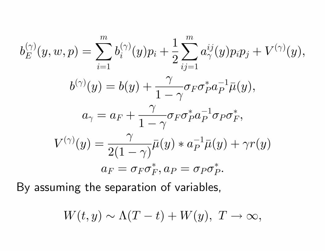
b(γ)E (y, w, p) =
m∑i=1
b(γ)i (y)pi +
12
m∑ij=1
aijγ (y)pipj + V (γ)(y),
b(γ)(y) = b(y) +γ
1− γσFσ
∗Pa
−1P µ(y),
aγ = aF +γ
1− γσFσ
∗Pa
−1P σPσ
∗F ,
V (γ)(y) =γ
2(1− γ)µ(y) ∗ a−1
P µ(y) + γr(y)
aF = σFσ∗F , aP = σPσ
∗P .
By assuming the separation of variables,
W (t, y) ∼ Λ(T − t) +W (y), T →∞,
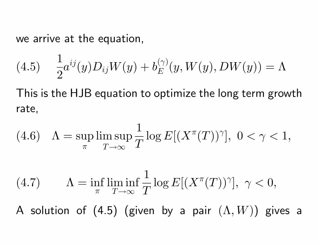
we arrive at the equation,
(4.5)12aij(y)DijW (y) + b
(γ)E (y,W (y), DW (y)) = Λ
This is the HJB equation to optimize the long term growth
rate,
(4.6) Λ = supπ
lim supT→∞
1T
logE[(Xπ(T ))γ], 0 < γ < 1,
(4.7) Λ = infπ
lim infT→∞
1T
logE[(Xπ(T ))γ], γ < 0,
A solution of (4.5) (given by a pair (Λ,W )) gives a
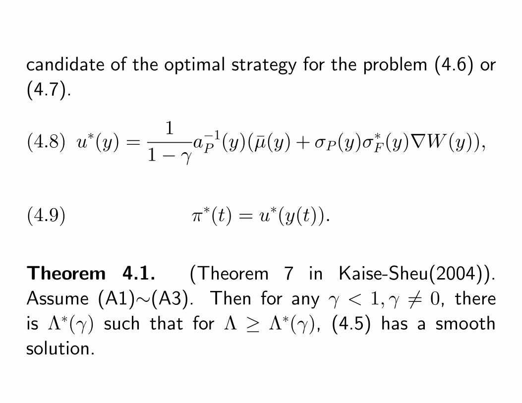
candidate of the optimal strategy for the problem (4.6) or
(4.7).
(4.8) u∗(y) =1
1− γa−1P (y)(µ(y) + σP(y)σ∗F(y)∇W (y)),
(4.9) π∗(t) = u∗(y(t)).
Theorem 4.1. (Theorem 7 in Kaise-Sheu(2004)).
Assume (A1)∼(A3). Then for any γ < 1, γ 6= 0, there
is Λ∗(γ) such that for Λ ≥ Λ∗(γ), (4.5) has a smooth
solution.
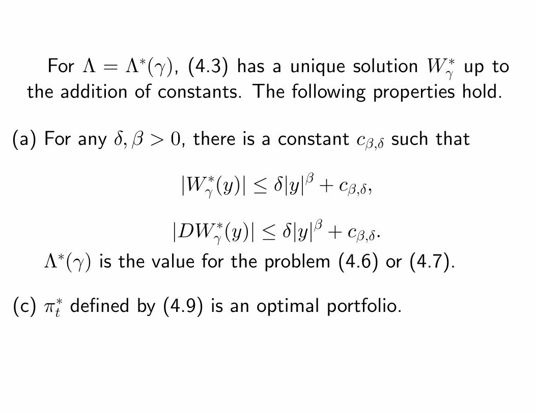
For Λ = Λ∗(γ), (4.3) has a unique solution W ∗γ up to
the addition of constants. The following properties hold.
(a) For any δ, β > 0, there is a constant cβ,δ such that
|W ∗γ (y)| ≤ δ|y|β + cβ,δ,
|DW ∗γ (y)| ≤ δ|y|β + cβ,δ.
Λ∗(γ) is the value for the problem (4.6) or (4.7).
(c) π∗t defined by (4.9) is an optimal portfolio.
5. Optimal Consumption Problem
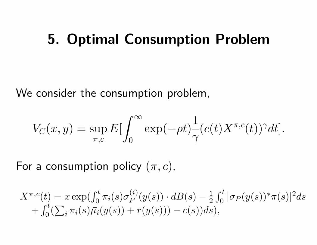
We consider the consumption problem,
VC(x, y) = supπ,c
E[∫ ∞
0exp(−ρt)1
γ(c(t)Xπ,c(t))γdt].
For a consumption policy (π, c),
Xπ,c(t) = x exp(∫ t
0πi(s)σ
(i)P (y(s)) · dB(s)− 1
2
∫ t
0|σP (y(s))∗π(s)|2ds
+∫ t
0(∑
i πi(s)µi(y(s)) + r(y(s)))− c(s))ds),
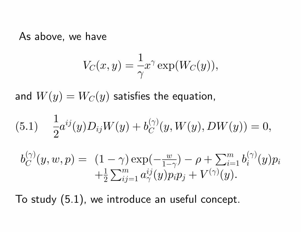
As above, we have
VC(x, y) =1γxγ exp(WC(y)),
and W (y) = WC(y) satisfies the equation,
(5.1)12aij(y)DijW (y) + b
(γ)C (y,W (y), DW (y)) = 0,
b(γ)C (y, w, p) = (1− γ) exp(− w
1−γ)− ρ+∑m
i=1 b(γ)i (y)pi
+12
∑mij=1 a
ijγ (y)pipj + V (γ)(y).
To study (5.1), we introduce an useful concept.
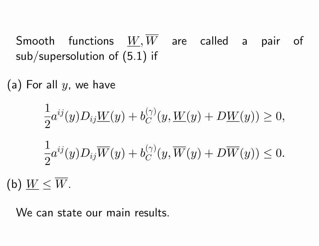
Smooth functions W,W are called a pair of
sub/supersolution of (5.1) if
(a) For all y, we have
12aij(y)DijW (y) + b
(γ)C (y,W (y) +DW (y)) ≥ 0,
12aij(y)DijW (y) + b
(γ)C (y,W (y) +DW (y)) ≤ 0.
(b) W ≤W .
We can state our main results.
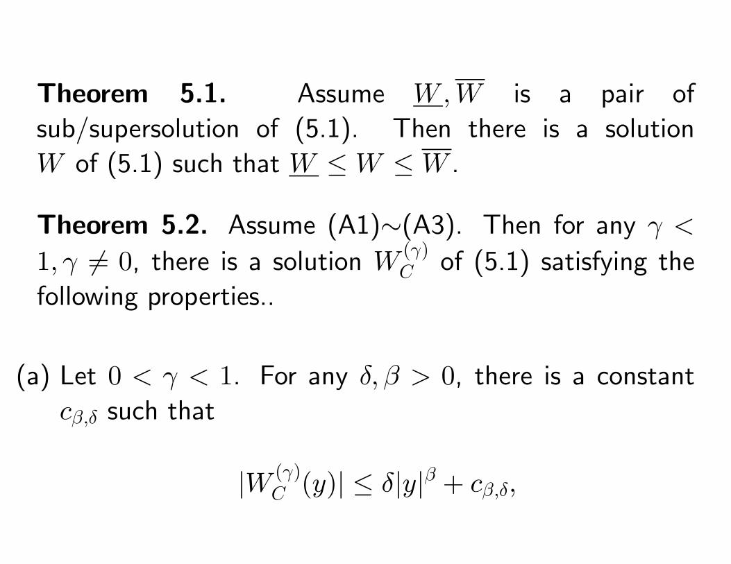
Theorem 5.1. Assume W,W is a pair of
sub/supersolution of (5.1). Then there is a solution
W of (5.1) such that W ≤W ≤W .
Theorem 5.2. Assume (A1)∼(A3). Then for any γ <
1, γ 6= 0, there is a solution W(γ)C of (5.1) satisfying the
following properties..
(a) Let 0 < γ < 1. For any δ, β > 0, there is a constant
cβ,δ such that
|W (γ)C (y)| ≤ δ|y|β + cβ,δ,
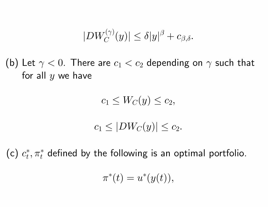
|DW (γ)C (y)| ≤ δ|y|β + cβ,δ.
(b) Let γ < 0. There are c1 < c2 depending on γ such that
for all y we have
c1 ≤WC(y) ≤ c2,
c1 ≤ |DWC(y)| ≤ c2.
(c) c∗t , π∗t defined by the following is an optimal portfolio.
π∗(t) = u∗(y(t)),
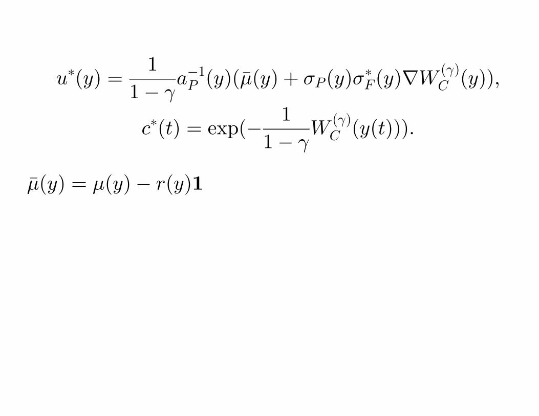
u∗(y) =1
1− γa−1P (y)(µ(y) + σP(y)σ∗F(y)∇W (γ)
C (y)),
c∗(t) = exp(− 11− γ
W(γ)C (y(t))).
µ(y) = µ(y)− r(y)1
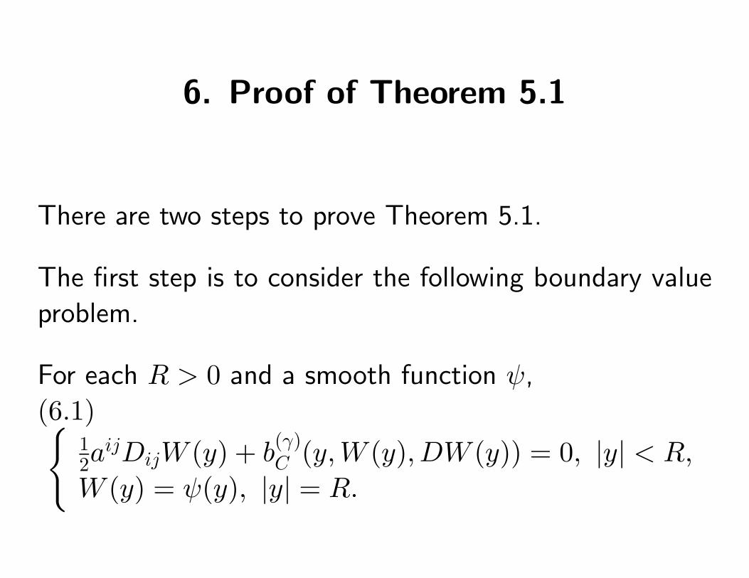
6. Proof of Theorem 5.1
There are two steps to prove Theorem 5.1.
The first step is to consider the following boundary value
problem.
For each R > 0 and a smooth function ψ,
(6.1){12a
ijDijW (y) + b(γ)C (y,W (y), DW (y)) = 0, |y| < R,
W (y) = ψ(y), |y| = R.
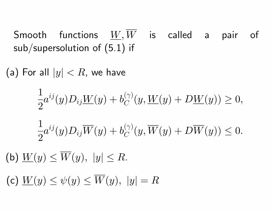
Smooth functions W,W is called a pair of
sub/supersolution of (5.1) if
(a) For all |y| < R, we have
12aij(y)DijW (y) + b
(γ)C (y,W (y) +DW (y)) ≥ 0,
12aij(y)DijW (y) + b
(γ)C (y,W (y) +DW (y)) ≤ 0.
(b) W (y) ≤W (y), |y| ≤ R.
(c) W (y) ≤ ψ(y) ≤W (y), |y| = R
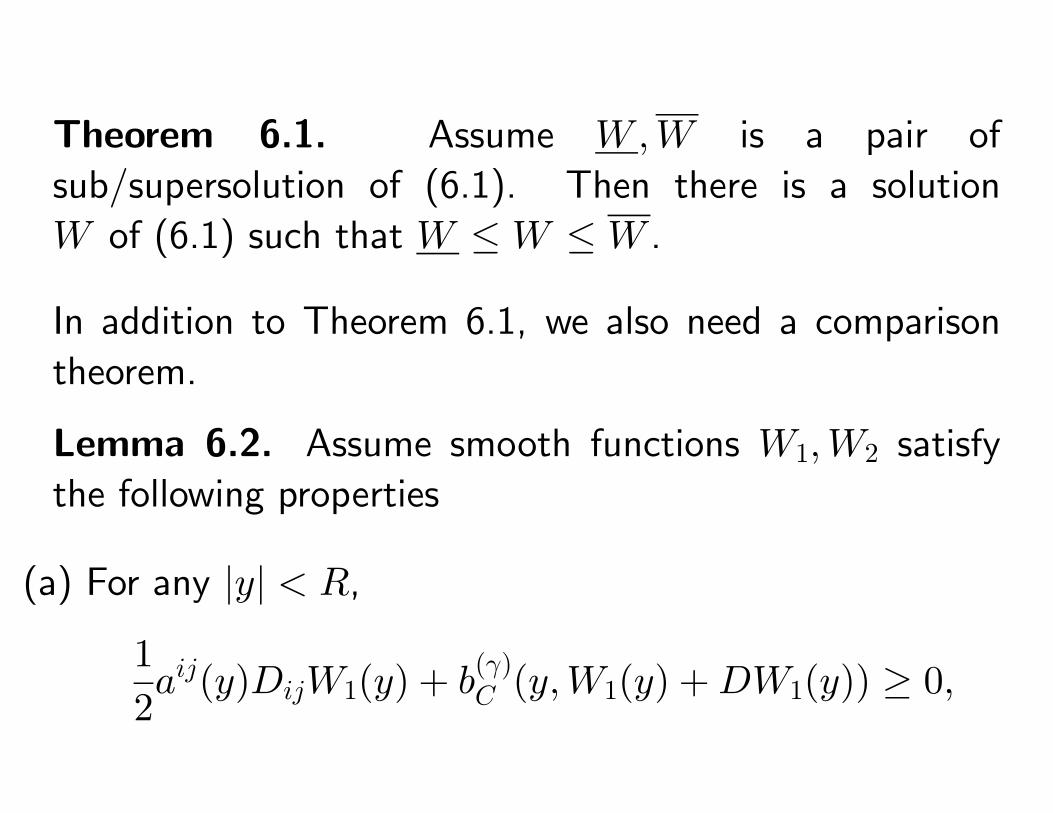
Theorem 6.1. Assume W,W is a pair of
sub/supersolution of (6.1). Then there is a solution
W of (6.1) such that W ≤W ≤W .
In addition to Theorem 6.1, we also need a comparison
theorem.
Lemma 6.2. Assume smooth functions W1,W2 satisfy
the following properties
(a) For any |y| < R,
12aij(y)DijW1(y) + b
(γ)C (y,W1(y) +DW1(y)) ≥ 0,
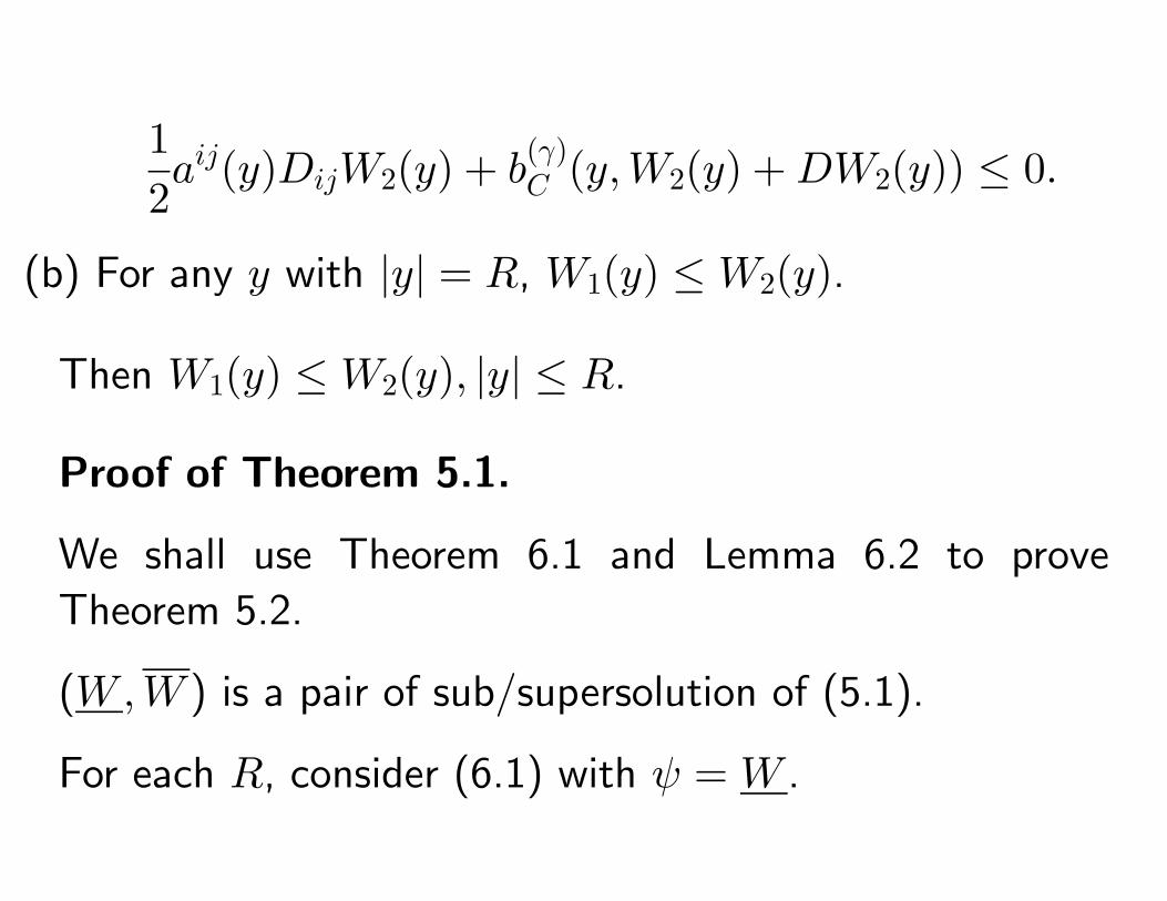
12aij(y)DijW2(y) + b
(γ)C (y,W2(y) +DW2(y)) ≤ 0.
(b) For any y with |y| = R, W1(y) ≤W2(y).
Then W1(y) ≤W2(y), |y| ≤ R.
Proof of Theorem 5.1.
We shall use Theorem 6.1 and Lemma 6.2 to prove
Theorem 5.2.
(W,W ) is a pair of sub/supersolution of (5.1).
For each R, consider (6.1) with ψ = W .
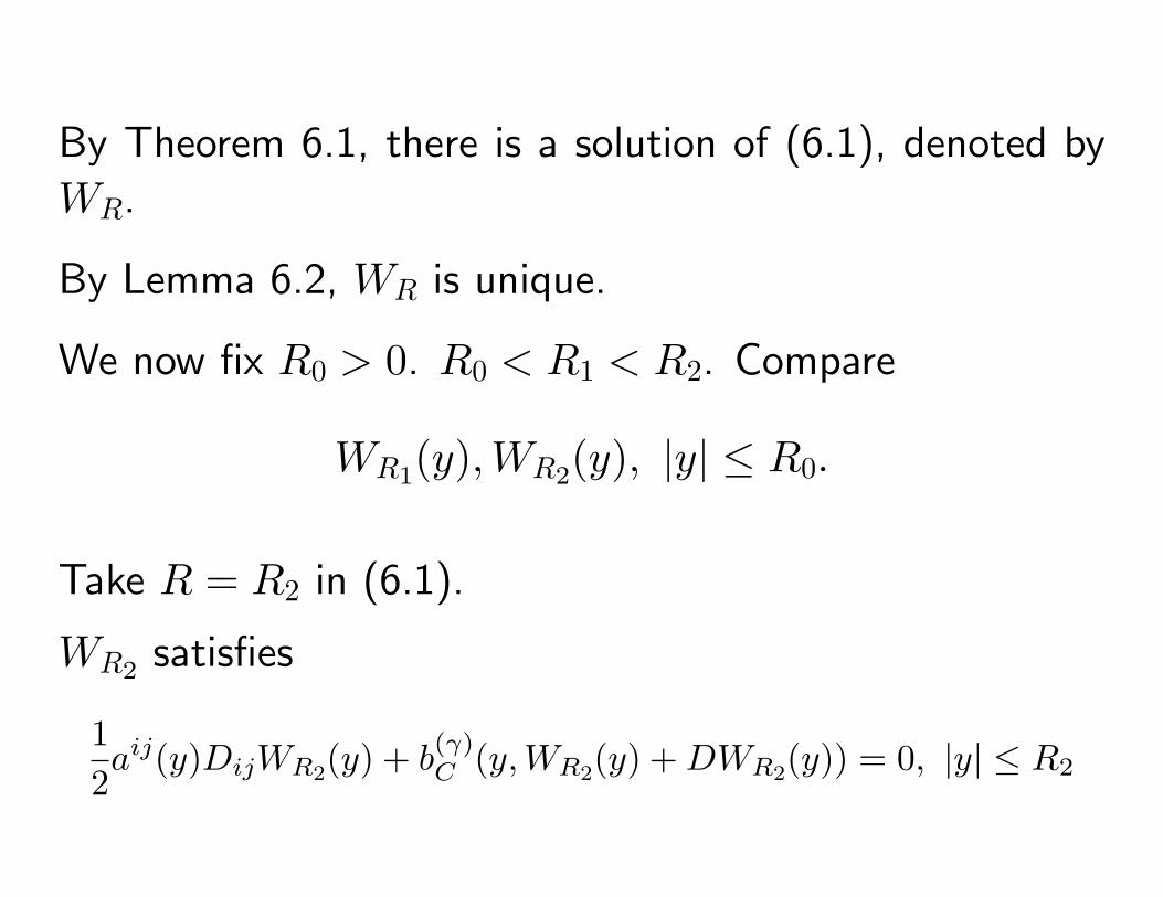
By Theorem 6.1, there is a solution of (6.1), denoted by
WR.
By Lemma 6.2, WR is unique.
We now fix R0 > 0. R0 < R1 < R2. Compare
WR1(y),WR2(y), |y| ≤ R0.
Take R = R2 in (6.1).
WR2 satisfies
12aij(y)DijWR2(y) + b
(γ)C (y,WR2(y) +DWR2(y)) = 0, |y| ≤ R2
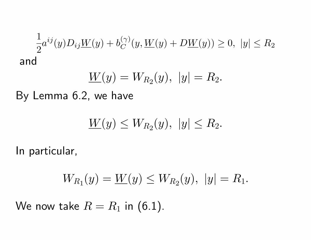
12aij(y)DijW (y) + b
(γ)C (y,W (y) +DW (y)) ≥ 0, |y| ≤ R2
and
W (y) = WR2(y), |y| = R2.
By Lemma 6.2, we have
W (y) ≤WR2(y), |y| ≤ R2.
In particular,
WR1(y) = W (y) ≤WR2(y), |y| = R1.
We now take R = R1 in (6.1).
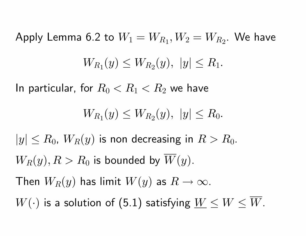
Apply Lemma 6.2 to W1 = WR1,W2 = WR2. We have
WR1(y) ≤WR2(y), |y| ≤ R1.
In particular, for R0 < R1 < R2 we have
WR1(y) ≤WR2(y), |y| ≤ R0.
|y| ≤ R0, WR(y) is non decreasing in R > R0.
WR(y), R > R0 is bounded by W (y).
Then WR(y) has limit W (y) as R→∞.
W (·) is a solution of (5.1) satisfying W ≤W ≤W .
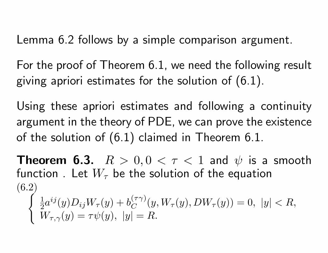
Lemma 6.2 follows by a simple comparison argument.
For the proof of Theorem 6.1, we need the following result
giving apriori estimates for the solution of (6.1).
Using these apriori estimates and following a continuity
argument in the theory of PDE, we can prove the existence
of the solution of (6.1) claimed in Theorem 6.1.
Theorem 6.3. R > 0, 0 < τ < 1 and ψ is a smoothfunction . Let Wτ be the solution of the equation(6.2){
12a
ij(y)DijWτ(y) + b(τγ)C (y,Wτ(y), DWτ(y)) = 0, |y| < R,
Wτ,γ(y) = τψ(y), |y| = R.
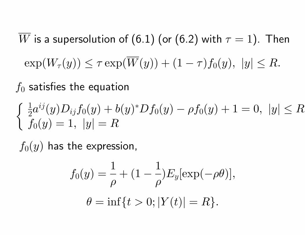
W is a supersolution of (6.1) (or (6.2) with τ = 1). Then
exp(Wτ(y)) ≤ τ exp(W (y)) + (1− τ)f0(y), |y| ≤ R.
f0 satisfies the equation{ 12a
ij(y)Dijf0(y) + b(y)∗Df0(y)− ρf0(y) + 1 = 0, |y| ≤ R,
f0(y) = 1, |y| = R
f0(y) has the expression,
f0(y) =1ρ
+ (1− 1ρ)Ey[exp(−ρθ)],
θ = inf{t > 0; |Y (t)| = R}.
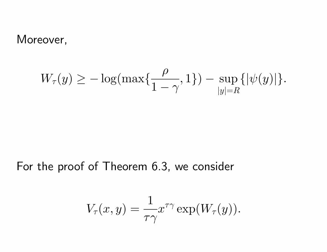
Moreover,
Wτ(y) ≥ − log(max{ ρ
1− γ, 1})− sup
|y|=R{|ψ(y)|}.
For the proof of Theorem 6.3, we consider
Vτ(x, y) =1τγxτγ exp(Wτ(y)).
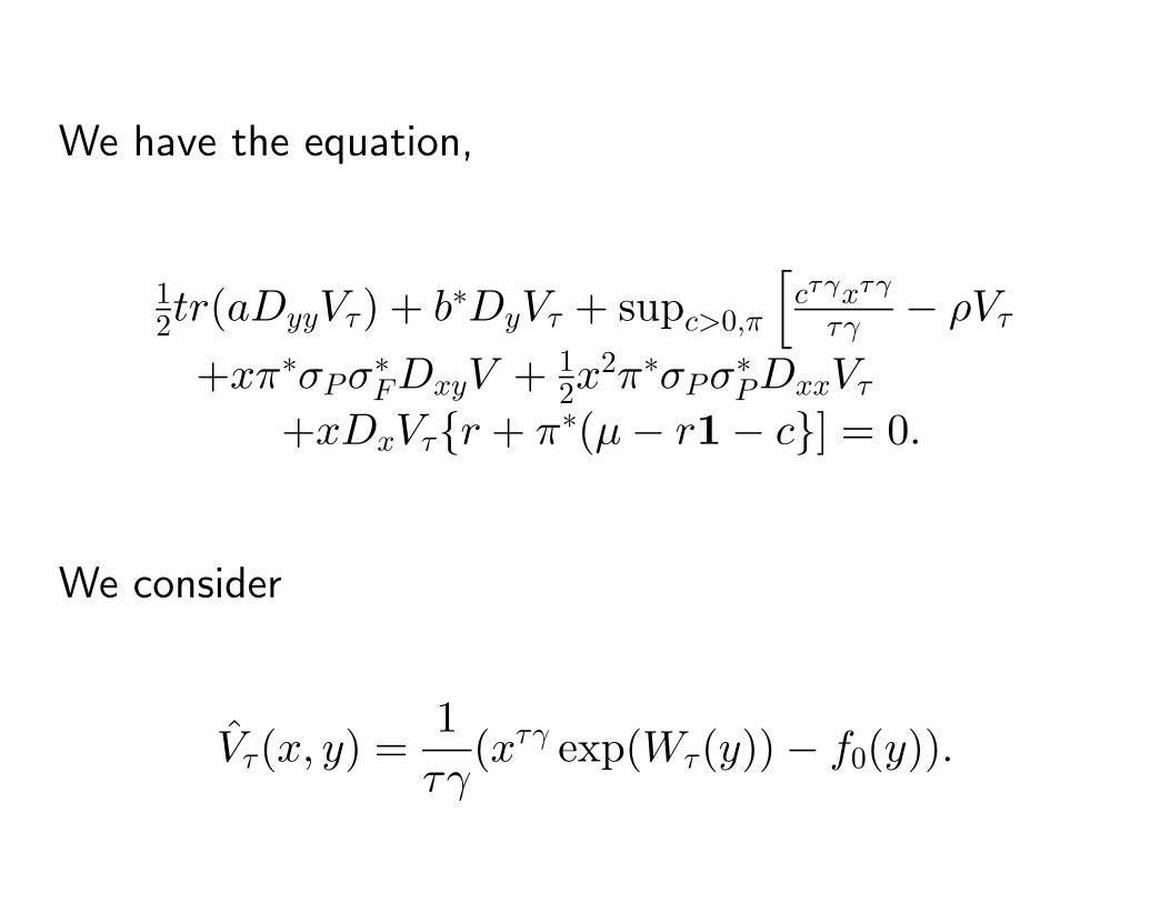
We have the equation,
12tr(aDyyVτ) + b∗DyVτ + supc>0,π
[cτγxτγ
τγ − ρVτ
+xπ∗σPσ∗FDxyV + 12x
2π∗σPσ∗PDxxVτ
+xDxVτ{r + π∗(µ− r1− c}] = 0.
We consider
Vτ(x, y) =1τγ
(xτγ exp(Wτ(y))− f0(y)).
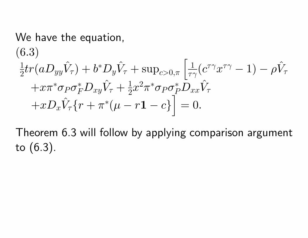
We have the equation,
(6.3)12tr(aDyyVτ) + b∗DyVτ + supc>0,π
[1τγ(c
τγxτγ − 1)− ρVτ
+xπ∗σPσ∗FDxyVτ + 12x
2π∗σPσ∗PDxxVτ
+xDxVτ{r + π∗(µ− r1− c}]
= 0.
Theorem 6.3 will follow by applying comparison argument
to (6.3).
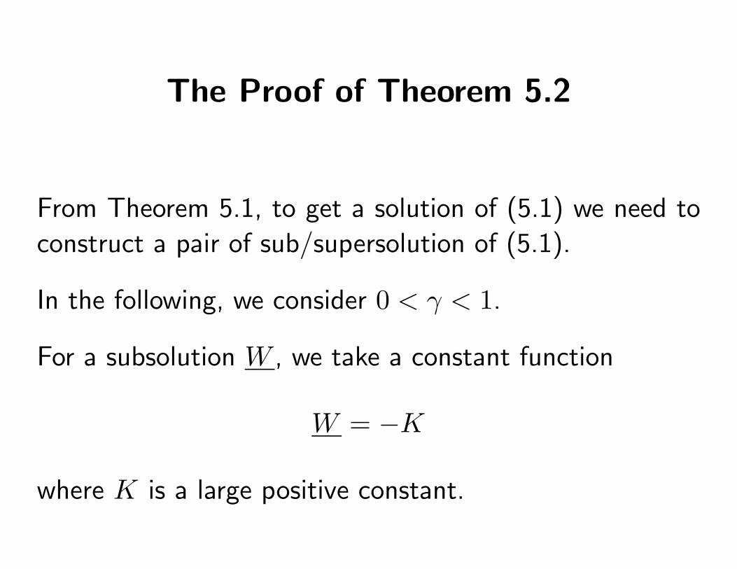
The Proof of Theorem 5.2
From Theorem 5.1, to get a solution of (5.1) we need to
construct a pair of sub/supersolution of (5.1).
In the following, we consider 0 < γ < 1.
For a subsolution W , we take a constant function
W = −K
where K is a large positive constant.
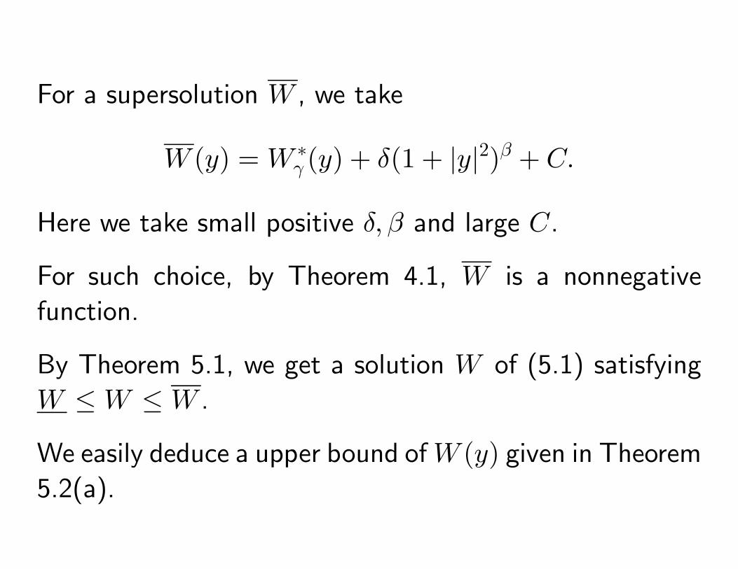
For a supersolution W , we take
W (y) = W ∗γ (y) + δ(1 + |y|2)β + C.
Here we take small positive δ, β and large C.
For such choice, by Theorem 4.1, W is a nonnegative
function.
By Theorem 5.1, we get a solution W of (5.1) satisfying
W ≤W ≤W .
We easily deduce a upper bound ofW (y) given in Theorem
5.2(a).
Using an idea in Kaise-Sheu (2004) and the upper estimate
of W , we can get an upper estimate of DW (y) as shown
in Theorem 5.2 (a).
Using the estimate in Theorem 5.2(a), we can prove the
verification theorem stated in Theorem 5.2(c).
The analysis for the case γ < 0 will be similar.