H-likelihood approach to high-dimensional multiple test

28 March 2015London, UK

Youngjo LeeSeoul National University

with Jan F. Bjϕrnstad, Donghwan Lee, Peirong Xu, Chris Frost,Gerard R. Ridgway, Mike Kenward, Rachael Scahill, Jianqing Shi

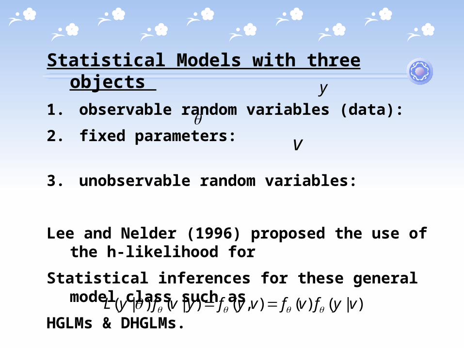
Statistical Models with three objects

1. observable random variables (data):

2. fixed parameters:

3. unobservable random variables:

Lee and Nelder (1996) proposed the use of the h-likelihood for

Statistical inferences for these general model class such as

HGLMs & DHGLMs.

y

v

)|()(),()|()|( vyfvfvyfyvfyL

Bj rnstad (1996)

The information in the data about unobservables, and parameters are in the extended likelihood such as the h-likelihood.

The h-likelihood gives inferences for both 1. parameters and 2. unobservables.

Multiple testing is a prediction problem of whether a null hypothesis is true or not!

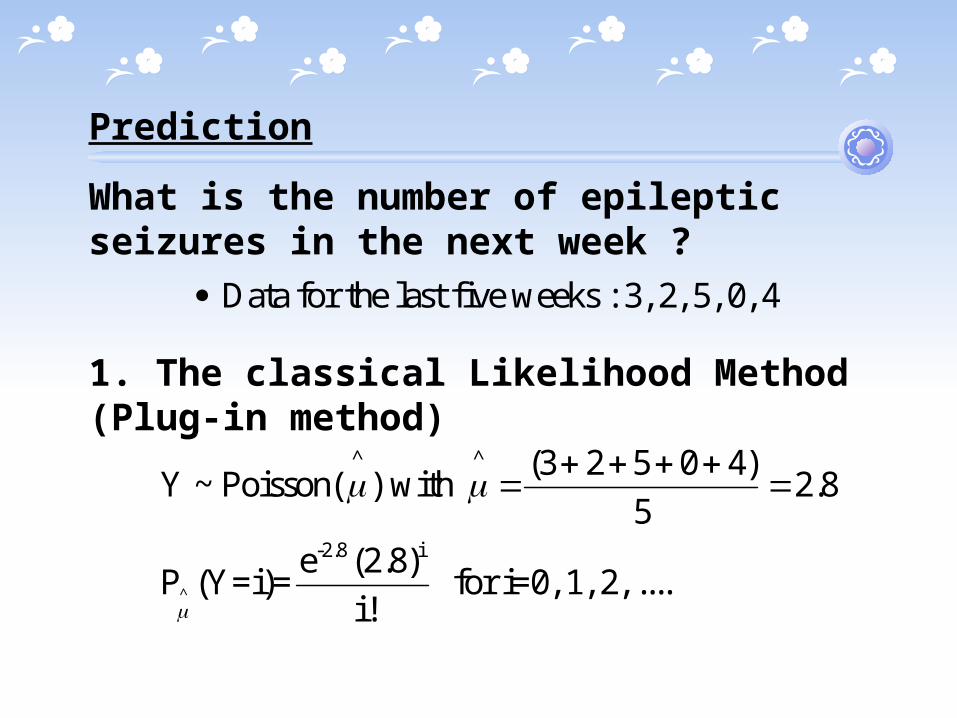
Prediction

What is the number of epileptic seizures in the next week ?

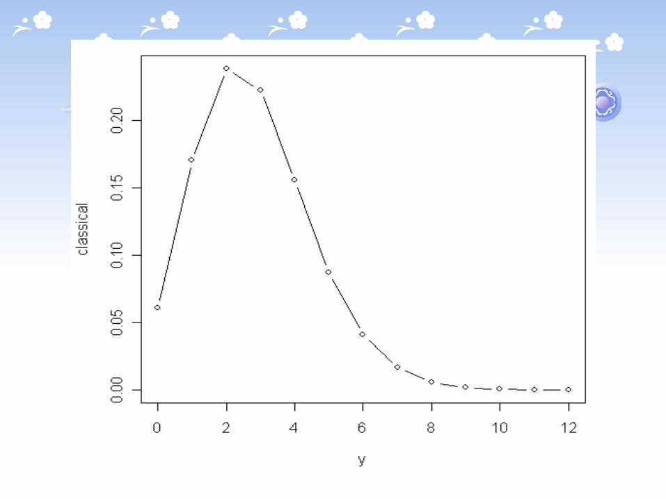
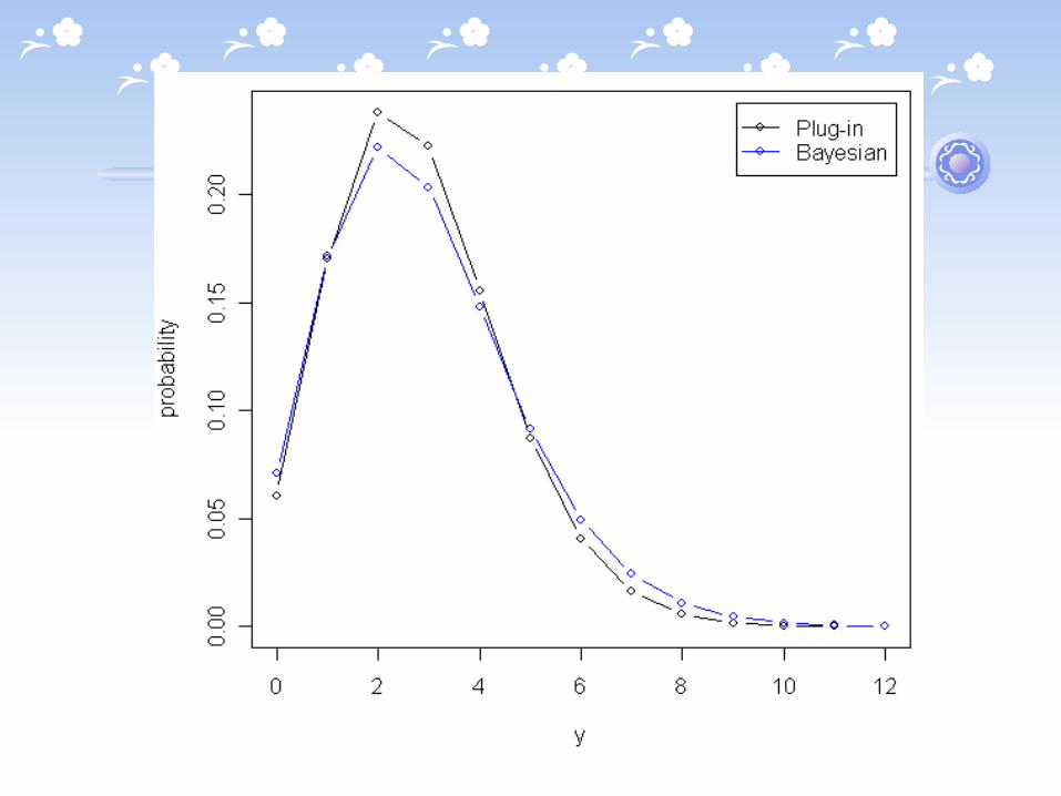
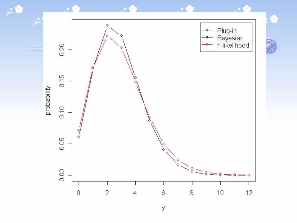
1. The classical Likelihood Method (Plug-in method)

Data for the last five weeks : 3, 2, 5, 0, 4

^

^ ^

-2.8 i

(3 2 5 0 4)Y ~ Poisson( ) with 2.8

5

e (2.8)P (Y=i)= for i=0, 1, 2, ....

i!

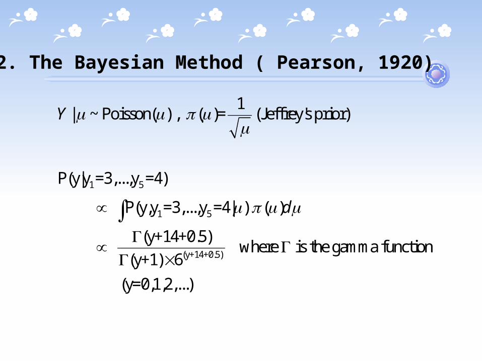
2. The Bayesian Method ( Pearson, 1920)

1 5

1 5

(y+14+0.5)

1| ~ Poisson( ) , ( )= (Jeffrey's prior)

P(y|y =3,...,y =4)

P(y,y =3,...,y =4| ) ( )

(y+14+0.5) where is the gamma function

(y+1) 6

Y

d

(y=0,1,2,...)

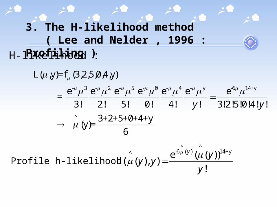
3. The H-likelihood method ( Lee and Nelder , 1996 : Profiling )

H-likelihood :

Profile h-likelihood :

^ ^-6 ( ) 14+y^ e ( ( ))

L( ( ), ) !

y yy y

y

- 3 - 2 - 5 - 0 - 4 - y -6 14+y

^

L( ,y)=f (3,2,5,0,4,y)

e e e e e e e =

3! 2! 5! 0! 4! ! 3!2!5!0!4! !

3+2+5+0+4+y (y)=

6

y y

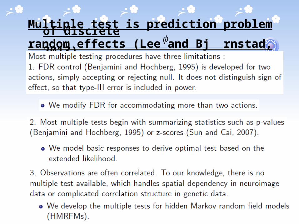
Multiple test is prediction problem of discreterandom effects (Lee and Bj rnstad, 2013)

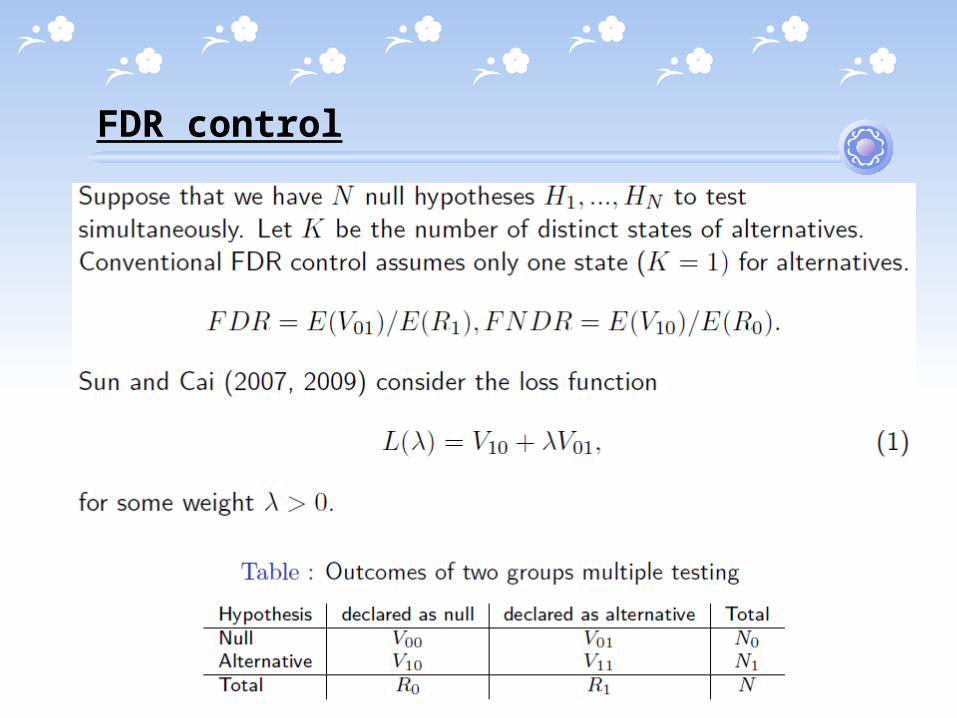
FDR control

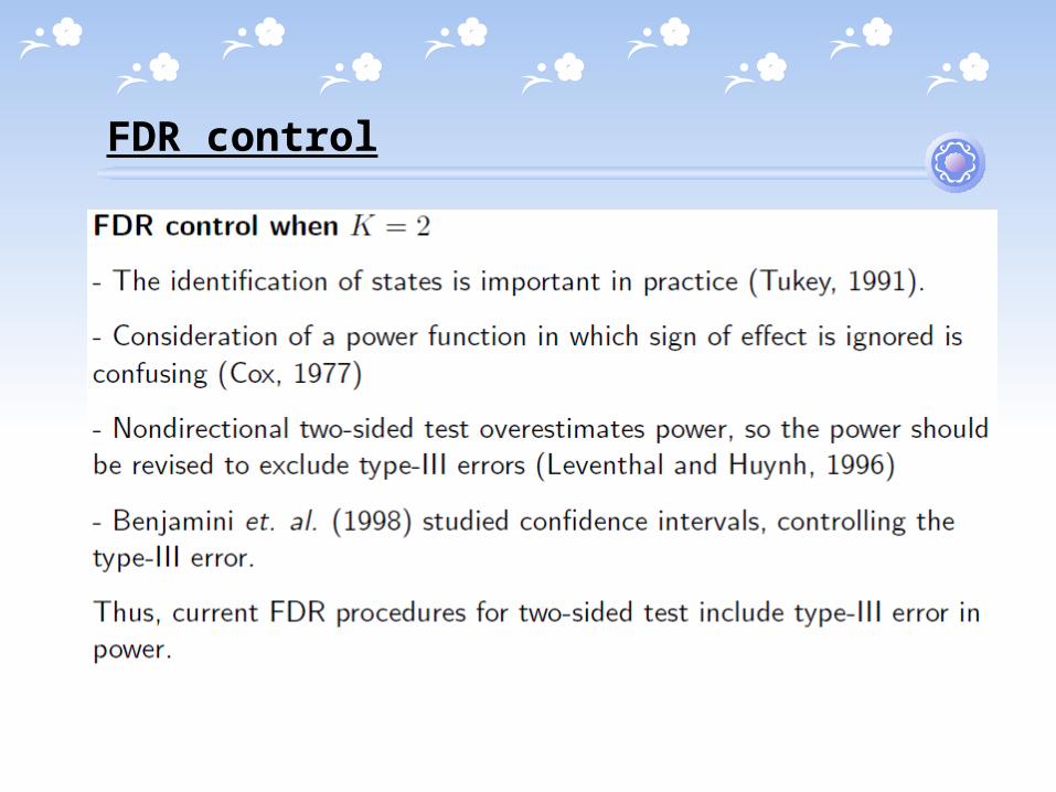
FDR control

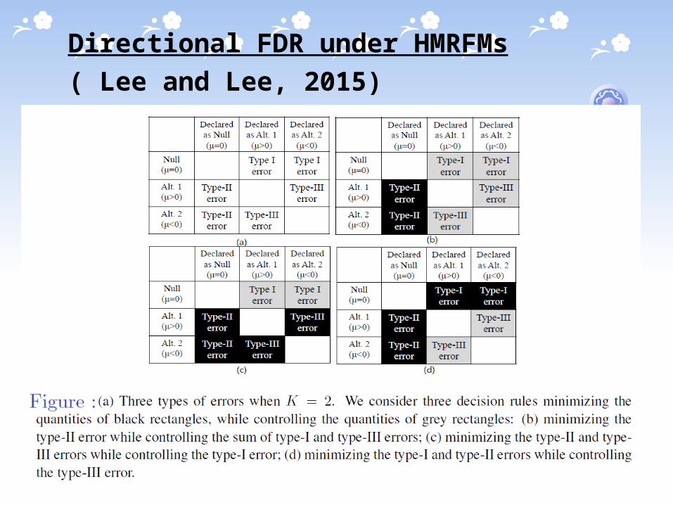
Directional FDR under HMRFMs

( Lee and Lee, 2015)

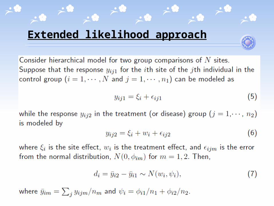
Extended likelihood approach

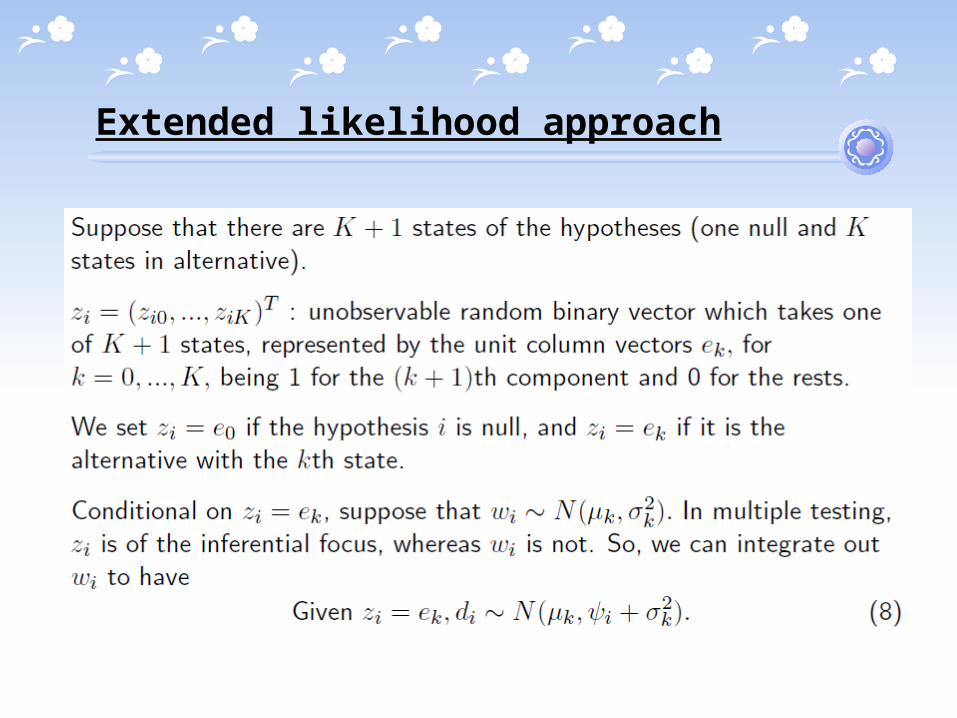
Extended likelihood approach

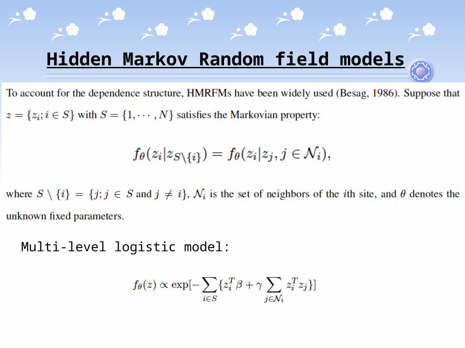
Hidden Markov Random field models

Multi-level logistic model:

Extended likelihood approach

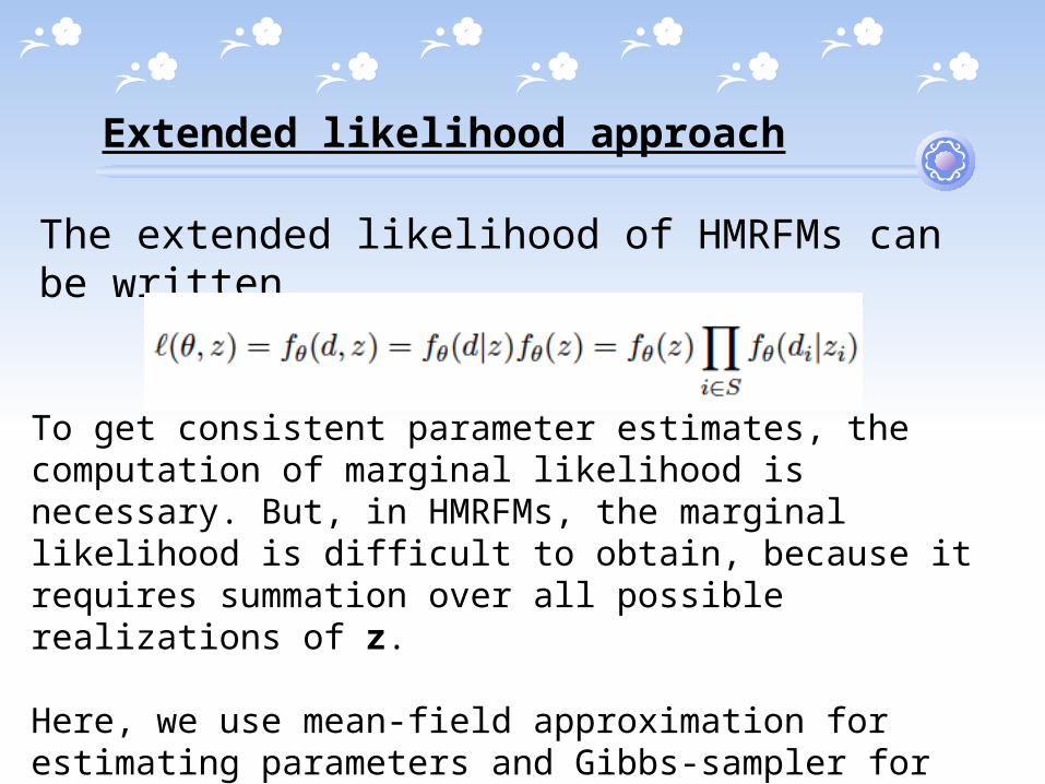
To get consistent parameter estimates, the computation of marginal likelihood is necessary. But, in HMRFMs, the marginal likelihood is difficult to obtain, because it requires summation over all possible realizations of z.

Here, we use mean-field approximation for estimating parameters and Gibbs-sampler for calculating directional error rates.

The extended likelihood of HMRFMs can be written

Extended likelihood approach

Extended likelihood approach

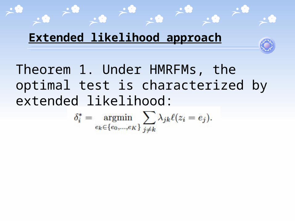
Theorem 1. Under HMRFMs, the optimal test is characterized by extended likelihood:

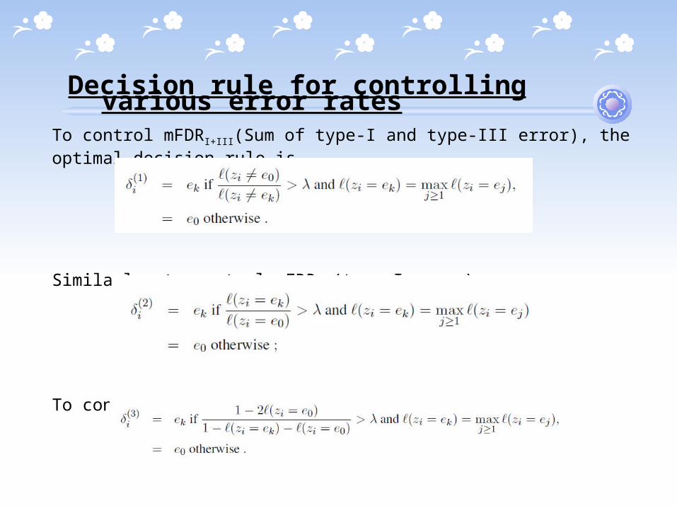
Decision rule for controlling various error rates

To control mFDRI+III(Sum of type-I and type-III error), the optimal decision rule is

Similarly, to control mFDRI (type-I error),

To control mFDRIII (type-III error),

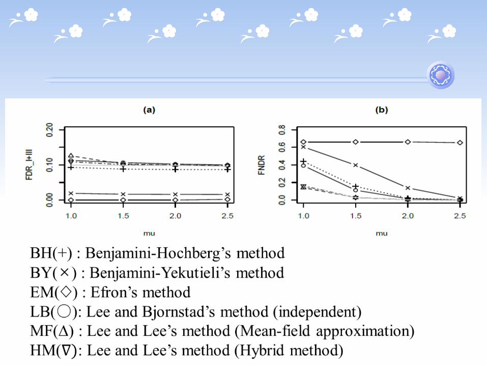
Numerical studies

One-sided test for Two-state hidden Markov models (1-dimensional)

 

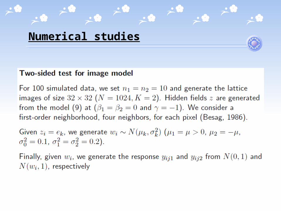
Numerical studies

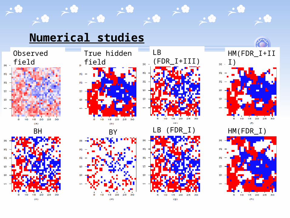
Numerical studiesObserved field True hidden field LB (FDR_I+III) HM(FDR_I+III)

LB (FDR_I) HM(FDR_I)BH BY

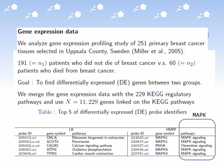
MAPK

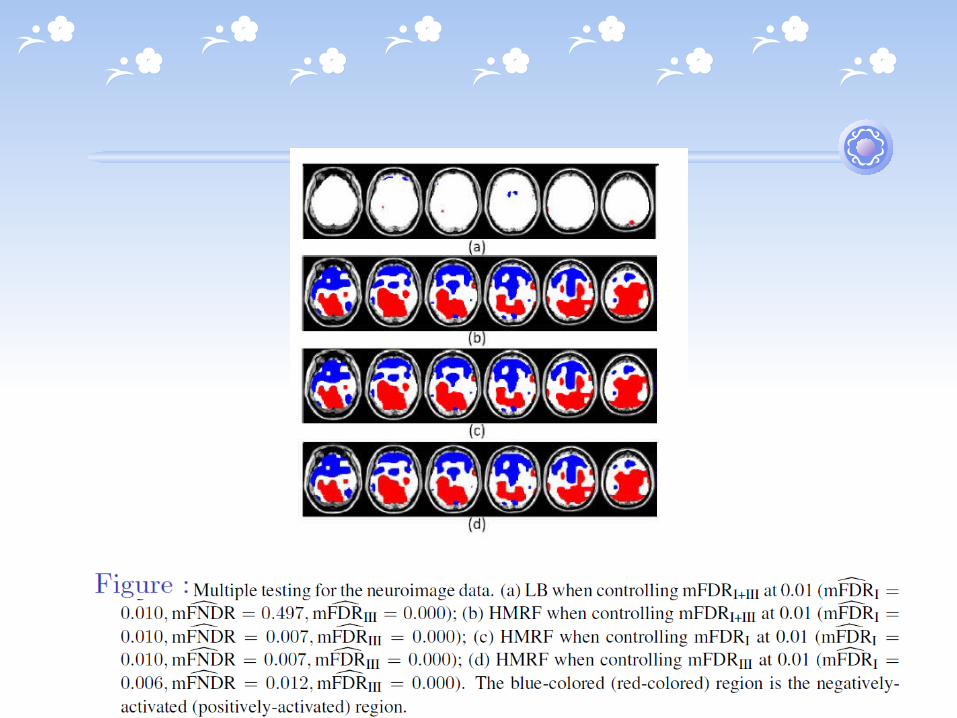
Neuroimage data example

Positron emission tomography (PET) data (Lee and Bjornstad, 2013)

28 healthy males v.s. 22 females.

Each PET images have N= 189,201 voxels.

Goal : To find the significantly different regions (voxels) of the brain between males and females.

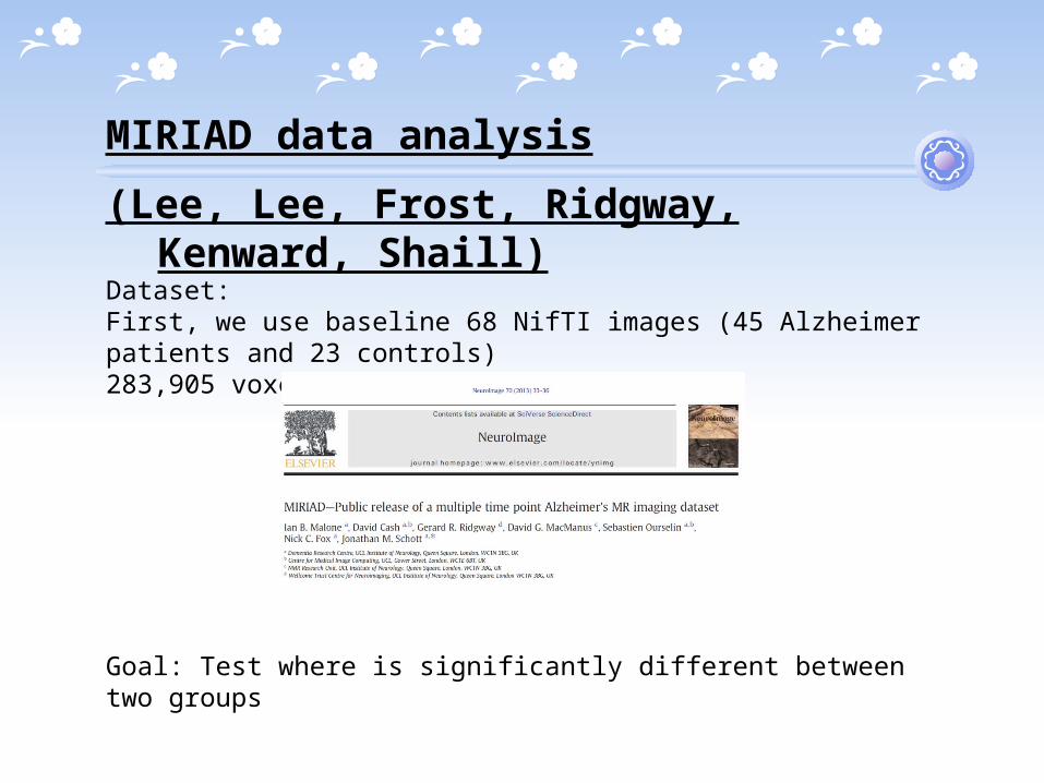
MIRIAD data analysis

(Lee, Lee, Frost, Ridgway, Kenward, Shaill)

Dataset: First, we use baseline 68 NifTI images (45 Alzheimer patients and 23 controls)283,905 voxels per image

Goal: Test where is significantly different between two groups

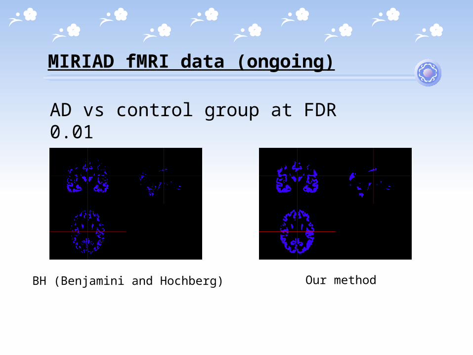
MIRIAD fMRI data (ongoing)

AD vs control group at FDR 0.01

BH (Benjamini and Hochberg) Our method

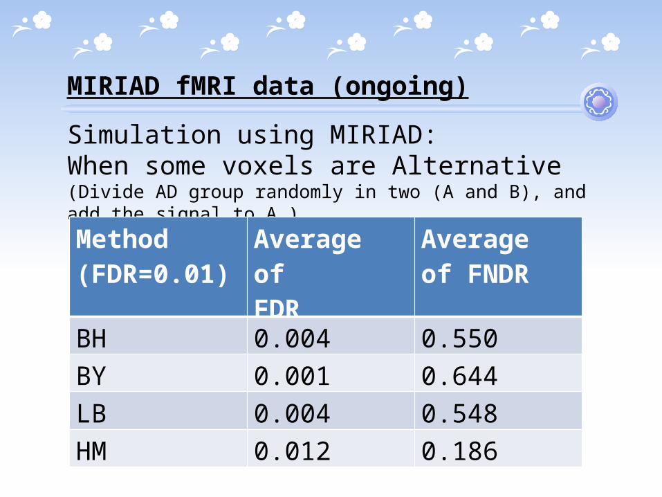
MIRIAD fMRI data (ongoing)

Simulation using MIRIAD: When some voxels are Alternative (Divide AD group randomly in two (A and B), and add the signal to A )

Method(FDR=0.01)

Average of FDR

Average of FNDR

BH 0.004 0.550BY 0.001 0.644LB 0.004 0.548HM 0.012 0.186

BLC mean correct latency data (Xu, Shi and Lee)

84 girls and 57 boys, aging from 6 to 13 years old.

Each student finished the Big/Little Circle (BLC) test via an action video game.

56% action video game players (AVGPs) v.s. 44% non-action video game players (NAVGPs).

Goal : To detect the areas of age automatically that the significant differences between AVGPs group and NAVGPs group occur.

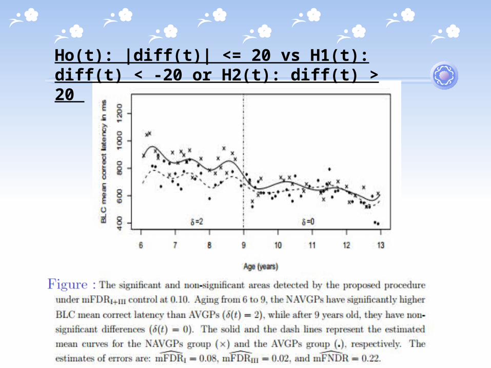
Ho(t): |diff(t)| <= 20 vs H1(t): diff(t) < -20 or H2(t): diff(t) > 20

Concluding remarks

When the null hypothesis is rejected it is important to control er-rors of incorrectly inferring the direction of the effect (type-III error). We proposed three ways of modifying the conventional FDR to accommodate such a need. We recommend to report the estimated of all three errors even if we control a specific FDR.

We derive the optimal test under HMRFMs. In real data analy-sis, likelihood-ratio test selects a HMRFM as the final model, showing an evidence of dependency among the observations. Thus, it is important to search for the best-fitting model in order to enhance the performance of the multiple test.

Thank you !