Gyrokinetic Particle Simulation in Tokamak Core

Zhihong Lin

Department of Physics & Astronomy University of California, Irvine

SciDAC Winter School on Turbulent Transport and Energetic ParticleIrvine, 2005

Critical issue: Plasma Confinement

• Fusion power density: Pfusion ~ n2<σv> ~ n2T2

• Energy loss due to transport: Ploss ~ nT/τE

• Lawson criterion: fusion gain Q=Pfusion/Ploss~ nTτEnT limited by magnetohydrodynamics (MHD) stability condition

global energy confinement time: τ ~ a2/χglobal energy confinement time: τE ~ a2/χIgnition requires Q>>1

• Extrapolation of thermal conductivity χ into burning plasma regime is a critical issue for ITER and DEMO

Toroidal Geometry

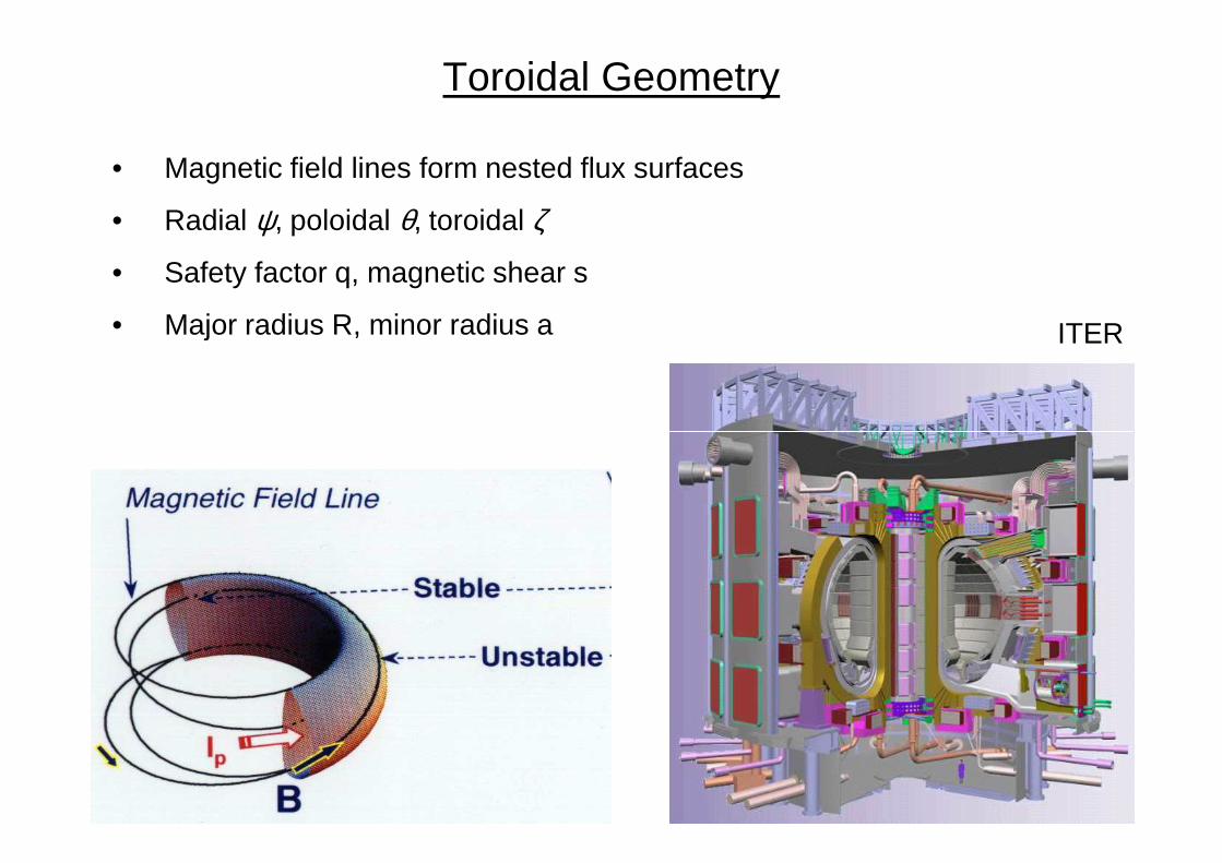
• Magnetic field lines form nested flux surfaces

• Radial ψ, poloidal θ, toroidal ζ

• Safety factor q, magnetic shear s

• Major radius R, minor radius a ITER

Guiding Center Orbit in Tokamak

• GC trajectories completely determined by conservation laws

Energy E=v2/2

Magnetic moment µ=mv2perp/2B

Toroidal canonical angular momentum pζ=Rmvζ-eψ

• Passing particle: orbit width=qρ, transit frequency ωt=v/qR

• Trapped particle: banana orbit• Trapped particle: banana orbit

Velocity pitch angle: p=v||/v <ε1/2

Trapped fraction: ε1/2

Orbit width: qρ/ε1/2

Bounce frequency: ωb= ε1/2v/qR

• Toroidal procession of trapped particle

Classical Transport

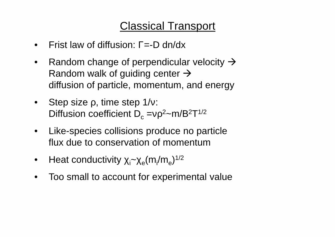
• Frist law of diffusion: Γ=-D dn/dx

• Random change of perpendicular velocity Random walk of guiding center diffusion of particle, momentum, and energy

• Step size ρ, time step 1/ν: Diffusion coefficient Dc =νρ2~m/B2T1/2Diffusion coefficient Dc =νρ ~m/B T

• Like-species collisions produce no particle flux due to conservation of momentum

• Heat conductivity χi~χe(mi/me)1/2

• Too small to account for experimental value

Neoclassical Transport

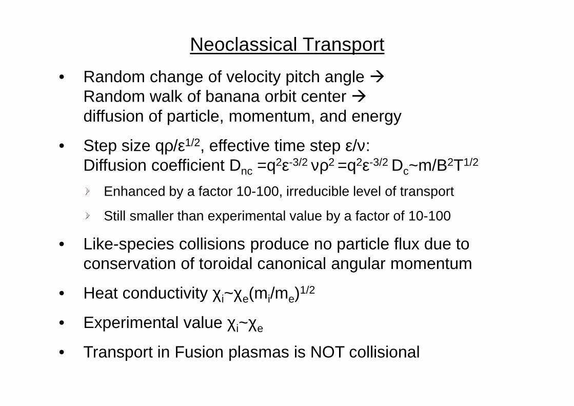
• Random change of velocity pitch angle Random walk of banana orbit center diffusion of particle, momentum, and energy

• Step size qρ/ε1/2, effective time step ε/ν: Diffusion coefficient Dnc =q2ε-3/2 νρ2 =q2ε-3/2 Dc~m/B2T1/2

Enhanced by a factor 10-100, irreducible level of transport

Still smaller than experimental value by a factor of 10-100

• Like-species collisions produce no particle flux due to conservation of toroidal canonical angular momentum

• Heat conductivity χi~χe(mi/me)1/2

• Experimental value χi~χe

• Transport in Fusion plasmas is NOT collisional

A Historical Perspective on Plasma Transport

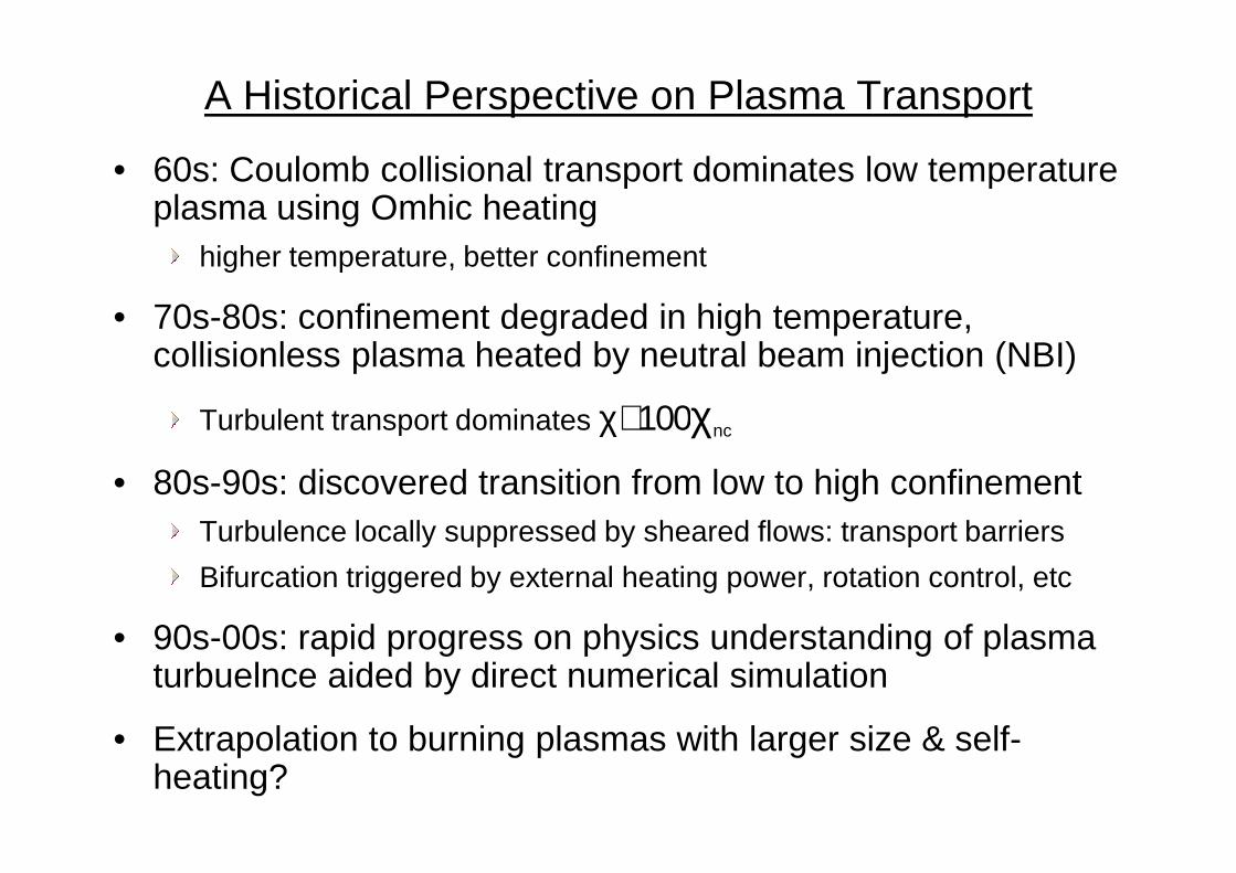
• 60s: Coulomb collisional transport dominates low temperature plasma using Omhic heating

higher temperature, better confinement

• 70s-80s: confinement degraded in high temperature, collisionless plasma heated by neutral beam injection (NBI)

Turbulent transport dominates χ∼100χncχ∼100χnc

• 80s-90s: discovered transition from low to high confinementTurbulence locally suppressed by sheared flows: transport barriers

Bifurcation triggered by external heating power, rotation control, etc

• 90s-00s: rapid progress on physics understanding of plasma turbuelnce aided by direct numerical simulation

• Extrapolation to burning plasmas with larger size & self-heating?

Transport Modeling vs. Physics Simulation

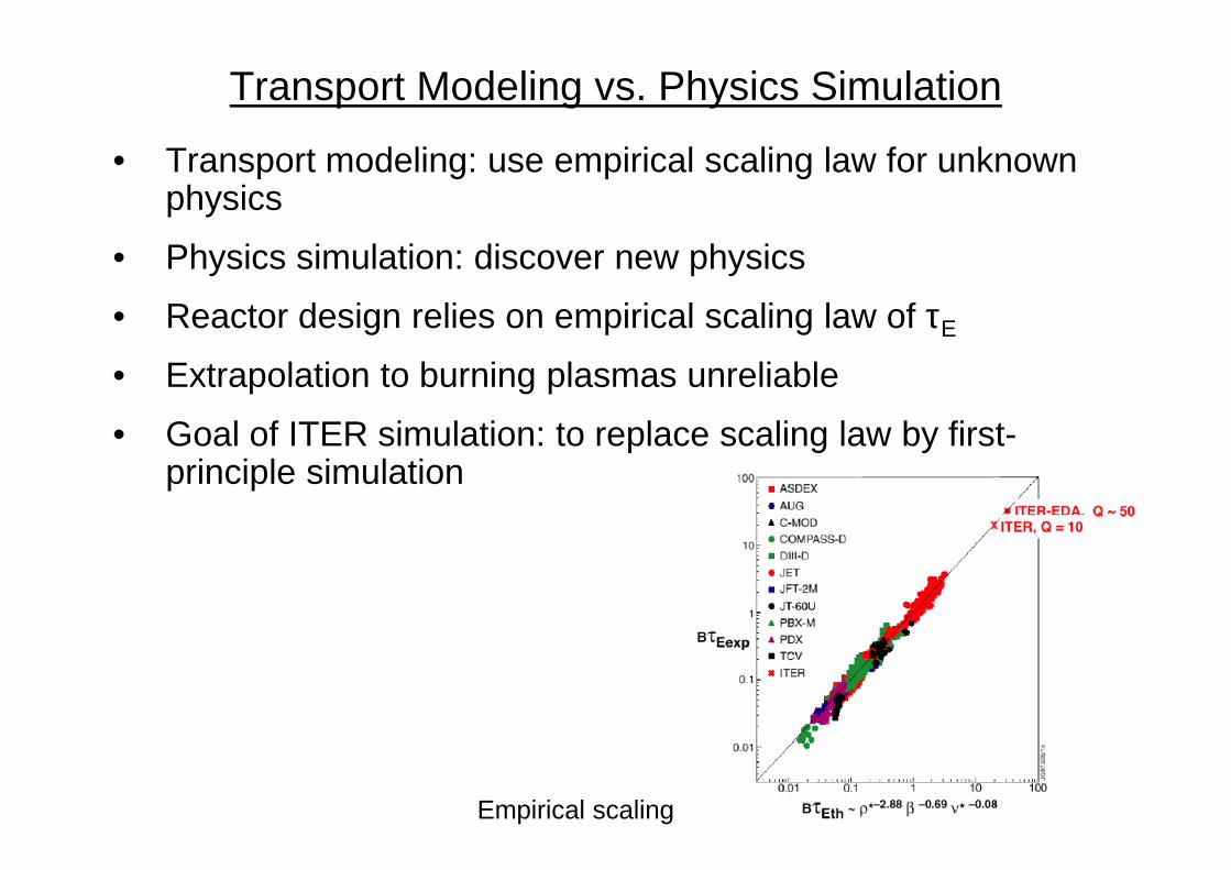
• Transport modeling: use empirical scaling law for unknown physics

• Physics simulation: discover new physics

• Reactor design relies on empirical scaling law of τE

• Extrapolation to burning plasmas unreliable

• Goal of ITER simulation: to replace scaling law by first-• Goal of ITER simulation: to replace scaling law by first-principle simulation

Empirical scaling

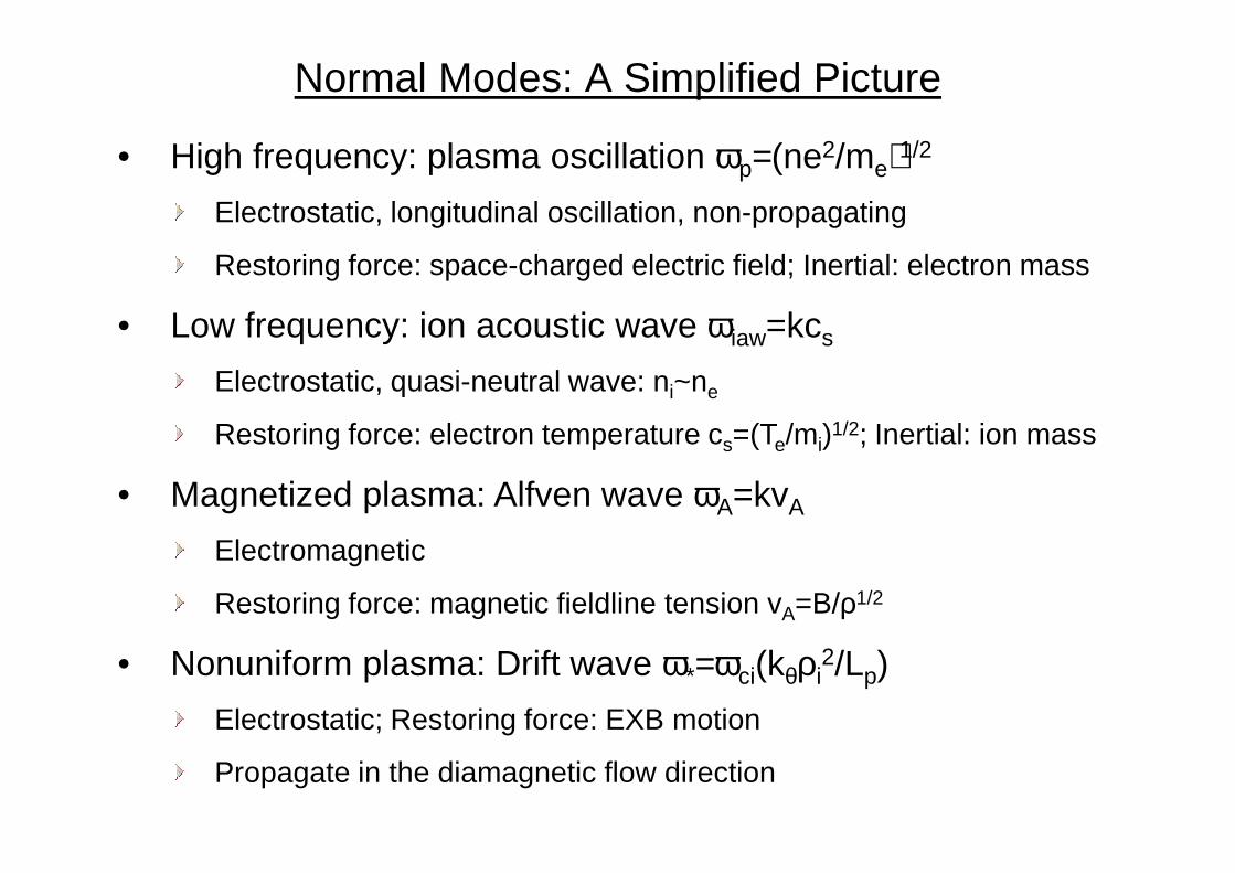
Normal Modes: A Simplified Picture

• High frequency: plasma oscillation ωp=(ne2/me)1/2

Electrostatic, longitudinal oscillation, non-propagating

Restoring force: space-charged electric field; Inertial: electron mass

• Low frequency: ion acoustic wave ωiaw=kcs

Electrostatic, quasi-neutral wave: ni~ne

Restoring force: electron temperature cs=(Te/mi)1/2; Inertial: ion massRestoring force: electron temperature cs=(Te/mi)1/2; Inertial: ion mass

• Magnetized plasma: Alfven wave ωA=kvA

Electromagnetic

Restoring force: magnetic fieldline tension vA=B/ρ1/2

• Nonuniform plasma: Drift wave ω*=ωci(kθρi2/Lp)

Electrostatic; Restoring force: EXB motion

Propagate in the diamagnetic flow direction

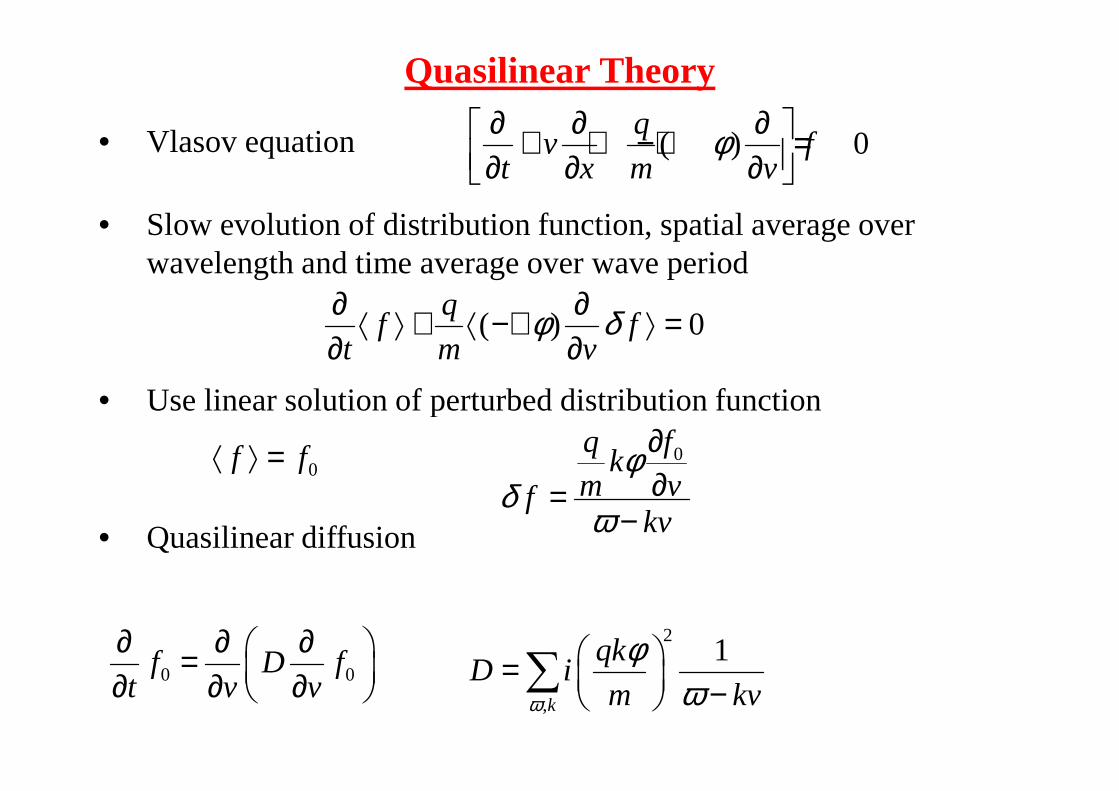
• Vlasov equation

• Slow evolution of distribution function, spatial average over wavelength and time average over wave period

• Use linear solution of perturbed distribution function

Quasilinear Theory

( ) 0q

v ft x m v

φ∂ ∂ ∂ + + −∇ = ∂ ∂ ∂

( ) 0q

f ft m v

φ δ∂ ∂⟨ ⟩ + ⟨ −∇ ⟩ =

∂ ∂• Use linear solution of perturbed distribution function

• Quasilinear diffusion

0q fk

m vfkv

φδ

ω

∂∂=

−

0f f⟨ ⟩ =

0 0f D ft v v

∂ ∂ ∂ = ∂ ∂ ∂

2

,

1

k

qkD i

m kvω

φω

= − ∑

Gyrokinetic Particle Simulation of Plasma Turbulence

• Linear micro-instabilities theory well understood & computationally “solved”

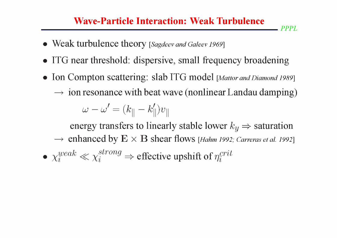
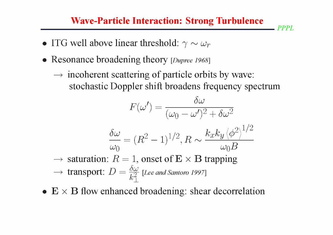
• Various nonlinear theories: applicable in limiting regimes

Wave-wave interactions: energy transfer to damped modes

Wave-particle interactions: Compton scattering, resonance broadening

• Particle simulations: treat all nonlinearities on same footing

Nonlinear wave-particle interactionsNonlinear wave-particle interactions

Complex geometry

• Gyrokinetic particle simulations of tokamak turbulence• Impacts of simulation on theory and experiment: zonal flow physics …

• US SciDAC: Scientific Discovery through Advanced Computing

• Core turbulent transport: GPS & GSPM

• Magnetohydrodynamics (MHD) instability: CEMM

• Radio-frequency (RF) heating: CSWPI

• Energetic particle turbulence and transport: GSEP

• US SciDAC FSP (Fusion Simulation Project): integrated simulation

Large Scale Simulation in Support of ITER

• US SciDAC FSP (Fusion Simulation Project): integrated simulation

• CPES: edge +MHD + atomic+…

• SWIM: MHD + RF

• FACETS: core + edge + wall

• FSP: project definition phase starts 2010

• EU ITM: Integrated Tokamak Modeling

• Japan BPSI: Burning Plasma Simulation Initiative

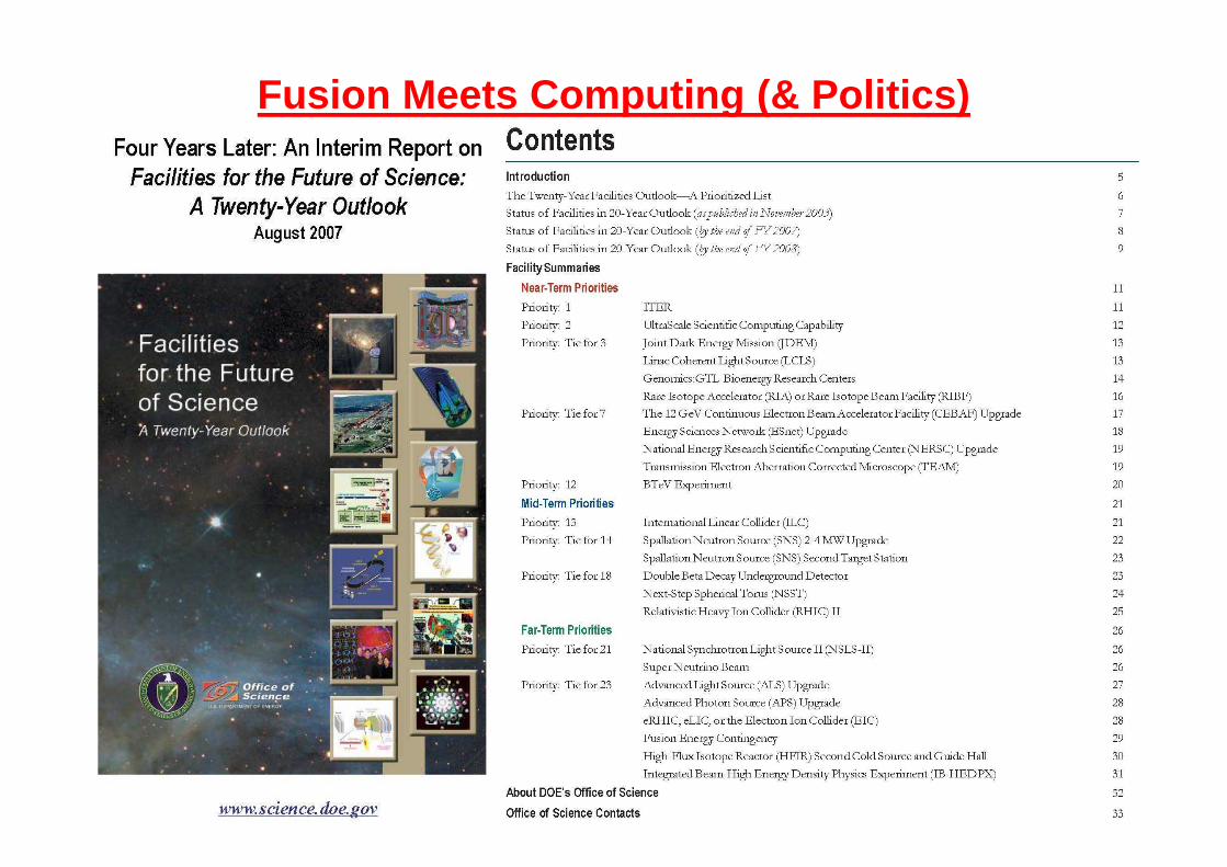
Fusion Meets Computing (& Politics)

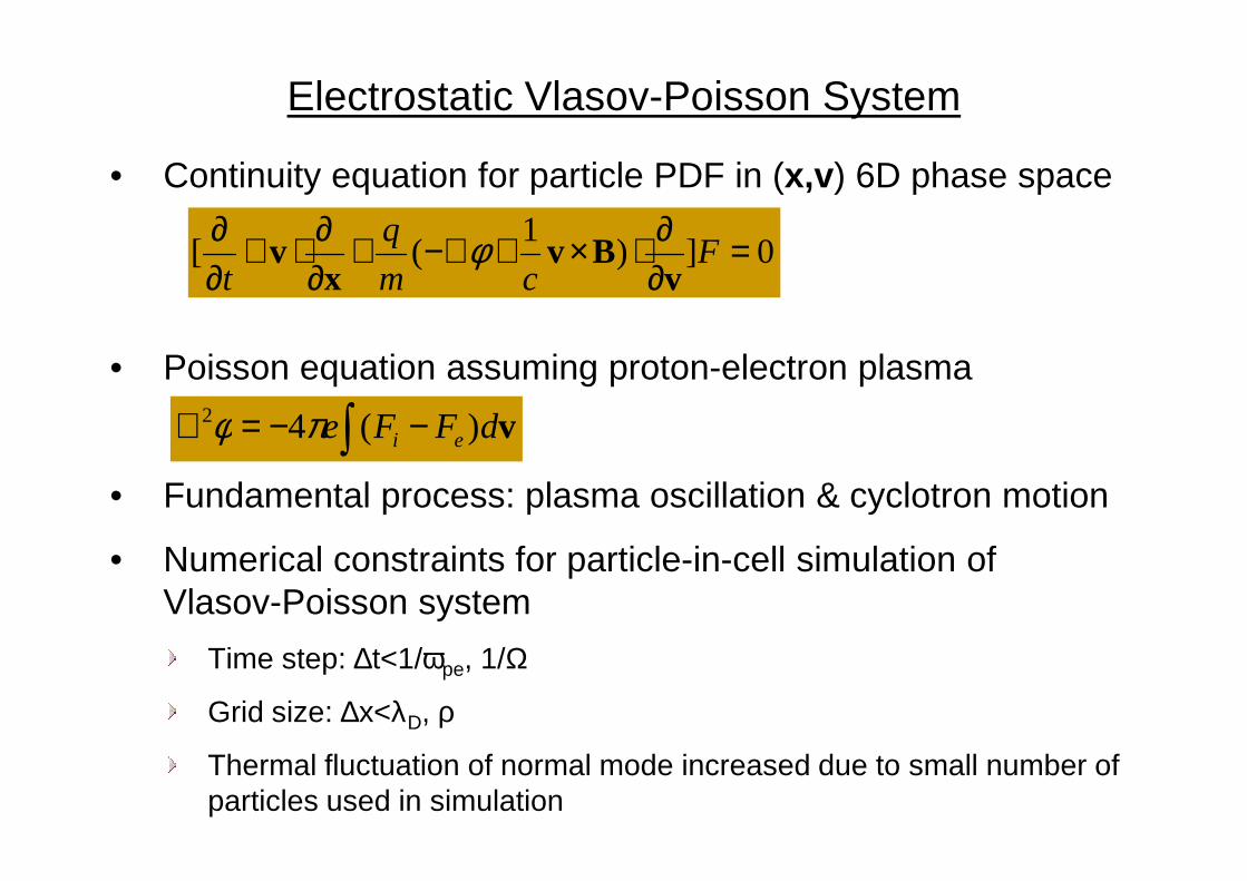
Electrostatic Vlasov-Poisson System

• Continuity equation for particle PDF in (x,v) 6D phase space

• Poisson equation assuming proton-electron plasma

0])1

([ =∂∂⋅×+−∇+

∂∂⋅+

∂∂

Fcm

q

t vBv

xv φ

∫ −−=∇ vdFFe ei )(42 πφ

• Fundamental process: plasma oscillation & cyclotron motion

• Numerical constraints for particle-in-cell simulation of Vlasov-Poisson system

Time step: ∆t<1/ωpe, 1/Ω

Grid size: ∆x<λD, ρ

Thermal fluctuation of normal mode increased due to small number of particles used in simulation

∫ −−=∇ vdFFe ei )(4πφ

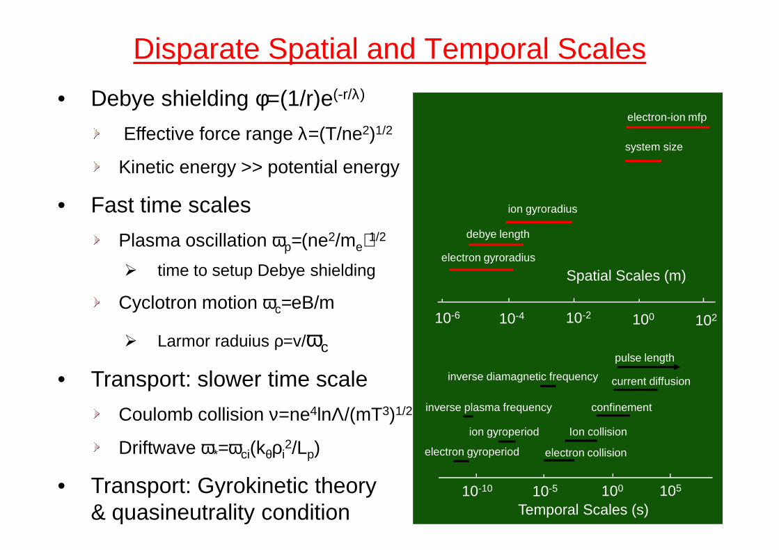
Disparate Spatial and Temporal Scales

Spatial Scales (m)electron gyroradius

debye length

ion gyroradius

system size

electron-ion mfp• Debye shielding φ=(1/r)e(-r/λ)

Effective force range λ=(T/ne2)1/2

Kinetic energy >> potential energy

• Fast time scales

Plasma oscillation ωp=(ne2/me)1/2

time to setup Debye shielding

10-6 10-4 10-2 100 102

Spatial Scales (m)

10-10 10-5 100 105

Temporal Scales (s)

electron gyroperiod electron collision

ion gyroperiod Ion collision

inverse plasma frequency confinement

current diffusion

pulse length

inverse diamagnetic frequency

time to setup Debye shielding

Cyclotron motion ωc=eB/m

Larmor raduius ρ=v/ωc

• Transport: slower time scale

Coulomb collision ν=ne4lnΛ/(mT3)1/2

Driftwave ω*=ωci(kθρi2/Lp)

• Transport: Gyrokinetic theory & quasineutrality condition

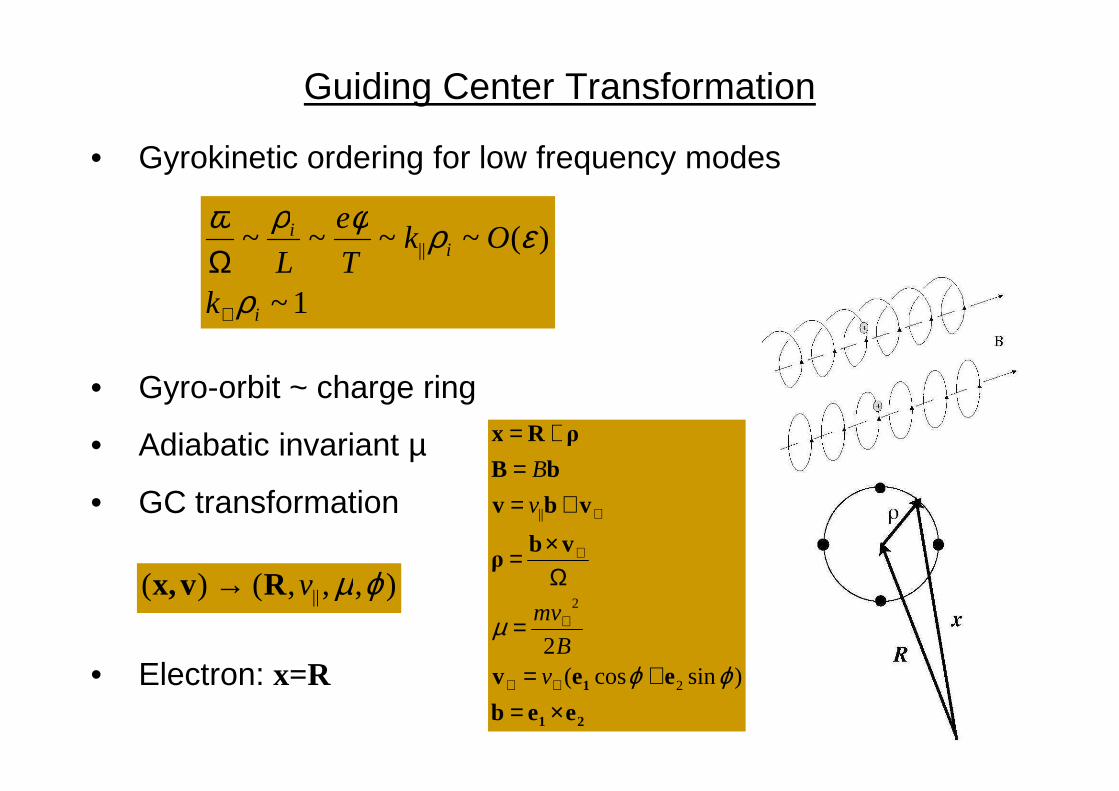
Guiding Center Transformation

• Gyrokinetic ordering for low frequency modes

• Gyro-orbit ~ charge ring

1~

)(~~~~ ||

i

ii

k

OkT

e

Lρ

ερφρω

⊥

Ω

• Gyro-orbit ~ charge ring

• Adiabatic invariant µ

• GC transformation

• Electron: x=R

),,,()( || ϕµvRvx, →

21

1

eeb

eev

vbρ

vbv

bB

ρRx

×=+=

=

Ω×=

+==

+=

⊥⊥

⊥

⊥

⊥

)sincos(2

2

2

||

ϕϕ

µ

vB

mv

v

B

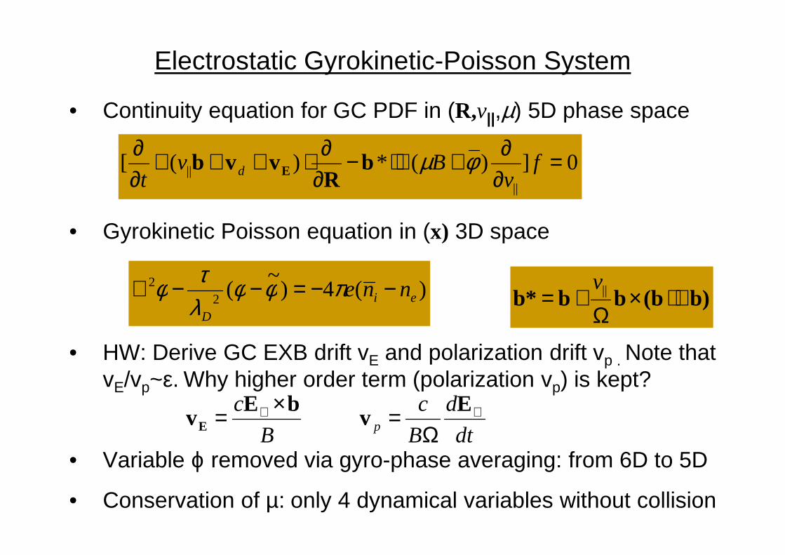
Electrostatic Gyrokinetic-Poisson System

• Continuity equation for GC PDF in (R,v||,µ) 5D phase space

• Gyrokinetic Poisson equation in (x) 3D space

0])(*)([||

|| =∂∂+⋅∇−

∂∂⋅+++

∂∂

fv

Bvt d φµb

Rvvb E

)(4)~

(2 nne −−=−−∇ πφφτφ v

• HW: Derive GC EXB drift vE and polarization drift vp . Note that vE/vp~ε. Why higher order term (polarization vp) is kept?

• Variable ϕ removed via gyro-phase averaging: from 6D to 5D

• Conservation of µ: only 4 dynamical variables without collision

)(4)~

(22

ei

D

nne −−=−−∇ πφφλτφ b)(bbbb* ∇⋅×

Ω+= ||v

B

c bEvE

×= ⊥

dt

d

B

cp

⊥

Ω= E

v

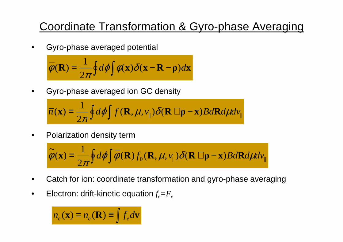
Coordinate Transformation & Gyro-phase Averaging

• Gyro-phase averaged potential

• Gyro-phase averaged ion GC density

|||| )(),,(2

1)( dvdBdvfdn µδµϕ

π ∫∫ −+= RxρRRx

∫∫ −−= xρRxxR dd )()(2

1)( δφϕ

πφ

• Polarization density term

• Catch for ion: coordinate transformation and gyro-phase averaging

• Electron: drift-kinetic equation fe=Fe

2π ∫∫

∫≡= vRx dfnn eee )()(

||||0 )(),,()(2

1)(

~dvdBdvfd µδµφϕ

πφ ∫∫ −+= RxρRRRx

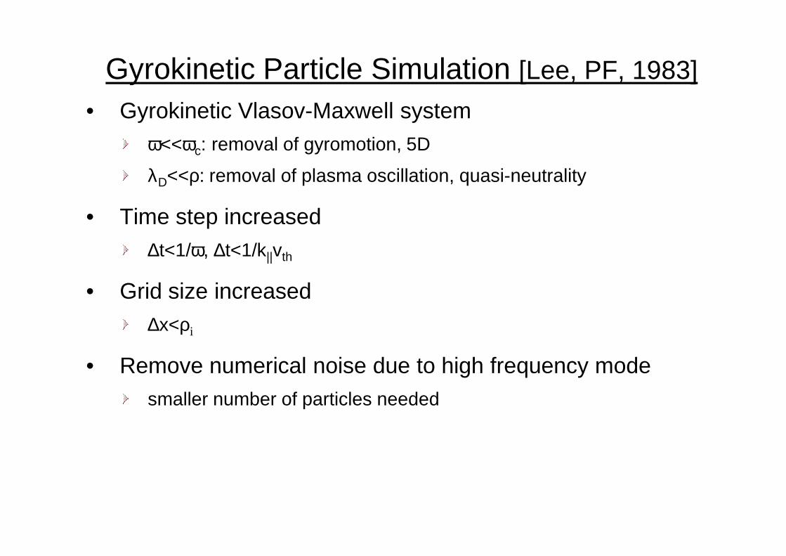
Gyrokinetic Particle Simulation [Lee, PF, 1983]

• Gyrokinetic Vlasov-Maxwell systemω<<ωc: removal of gyromotion, 5D

λD<<ρ: removal of plasma oscillation, quasi-neutrality

• Time step increased∆t<1/ω, ∆t<1/k||vth

• Grid size increased∆x<ρi

• Remove numerical noise due to high frequency modesmaller number of particles needed

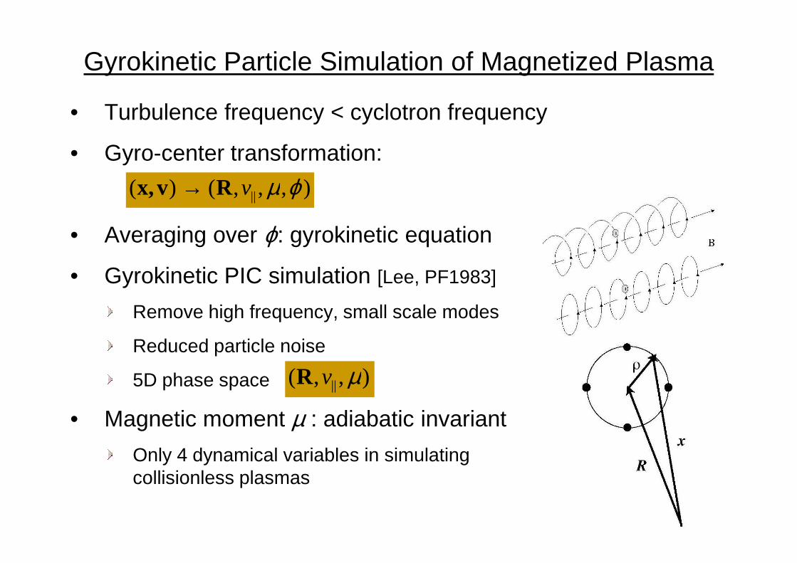
Gyrokinetic Particle Simulation of Magnetized Plasma

• Turbulence frequency < cyclotron frequency

• Gyro-center transformation:

• Averaging over ϕ: gyrokinetic equation

• Gyrokinetic PIC simulation [Lee, PF1983]

),,,()( || ϕµvRvx, →

• Gyrokinetic PIC simulation [Lee, PF1983]

Remove high frequency, small scale modes

Reduced particle noise

5D phase space

• Magnetic moment µ : adiabatic invariant

Only 4 dynamical variables in simulating collisionless plasmas

),,( || µvR

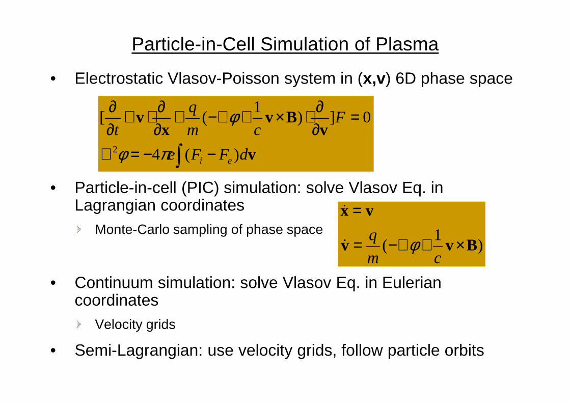
Particle-in-Cell Simulation of Plasma

• Electrostatic Vlasov-Poisson system in (x,v) 6D phase space

• Particle-in-cell (PIC) simulation: solve Vlasov Eq. in Lagrangian coordinates

∫ −−=∇

=∂∂⋅×+−∇+

∂∂⋅+

∂∂

v

vBv

xv

dFFe

Fcm

q

t

ei )(4

0])1

([

2 πφ

φ

Lagrangian coordinatesMonte-Carlo sampling of phase space

• Continuum simulation: solve Vlasov Eq. in Eulerian coordinates

Velocity grids

• Semi-Lagrangian: use velocity grids, follow particle orbits

)1

( Bvv

vx

×+−∇=

=

cm

q φ&

&

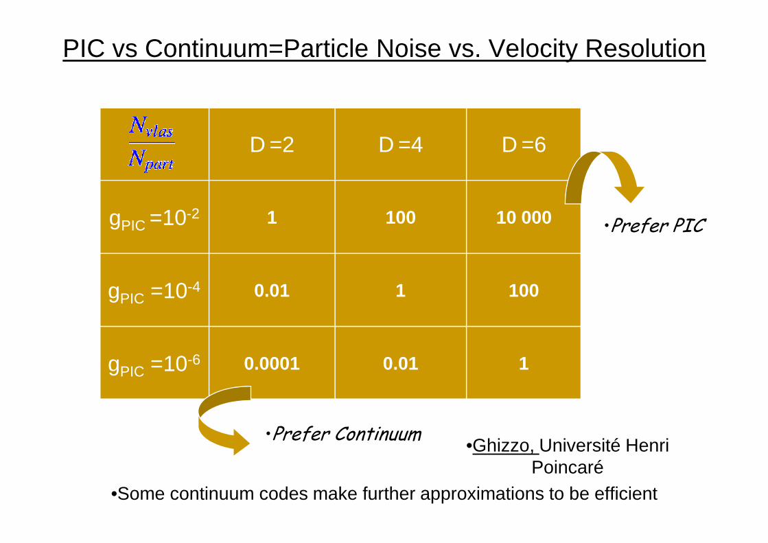
PIC vs Continuum=Particle Noise vs. Velocity Resolution

D =2 D =4 D =6

gPIC =10-2 1 100 10 000•Prefer PIC

gPIC =10-4 0.01 1 100

gPIC =10-6 0.0001 0.01 1

•Prefer Continuum

•Some continuum codes make further approximations to be efficient

•Ghizzo, Université Henri Poincaré

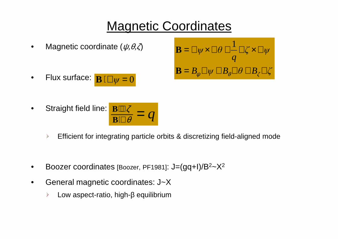
Magnetic Coordinates

• Magnetic coordinate (ψ,θ,ζ)

• Flux surface:

• Straight field line:

ζBθBψB

ψζq

θψ

∇+∇+∇=

∇×∇+∇×∇=

ζθψB

B1

0=∇⋅ ψB

q=∇⋅∇⋅

θζ

BB

Efficient for integrating particle orbits & discretizing field-aligned mode

• Boozer coordinates [Boozer, PF1981]: J=(gq+I)/B2~X2

• General magnetic coordinates: J~X

Low aspect-ratio, high-β equilibrium

q=∇⋅ θB

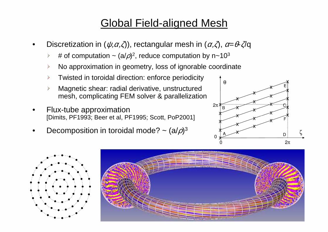
Global Field-aligned Mesh

• Discretization in (ψ,α,ζ)), rectangular mesh in (α,ζ), α=θ-ζ/q# of computation ~ (a/ρ)2, reduce computation by n~103

No approximation in geometry, loss of ignorable coordinate

Twisted in toroidal direction: enforce periodicity

Magnetic shear: radial derivative, unstructured mesh, complicating FEM solver & parallelization

• Flux-tube approximation [Dimits, PF1993; Beer et al, PF1995; Scott, PoP2001][Dimits, PF1993; Beer et al, PF1995; Scott, PoP2001]

• Decomposition in toroidal mode? ~ (a/ρ)3

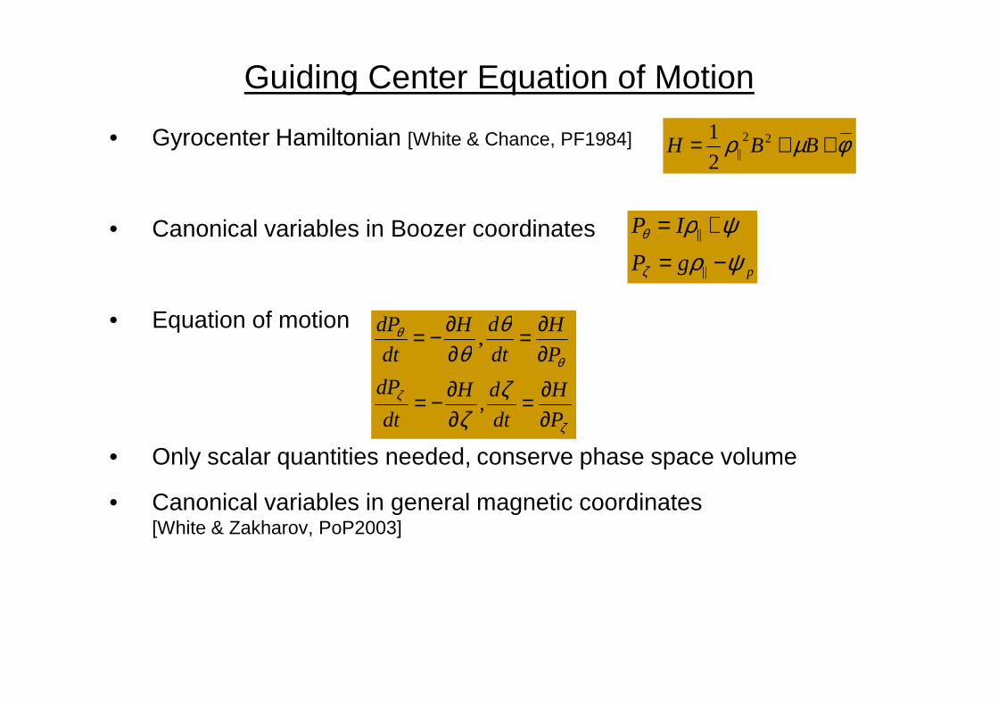
Guiding Center Equation of Motion

• Gyrocenter Hamiltonian [White & Chance, PF1984]

• Canonical variables in Boozer coordinates

• Equation of motion

φµρ ++= BBH 22||2

1

pgP

IP

ψρψρ

ζ

θ

−=

+=

||

||

θ θθ P

H

dt

dH

dt

dP

∂∂=

∂∂−= ,

• Only scalar quantities needed, conserve phase space volume

• Canonical variables in general magnetic coordinates [White & Zakharov, PoP2003]

ζ

ζ

θ

ζζ

θ

P

H

dt

dH

dt

dP

Pdtdt

∂∂=

∂∂−=

∂∂

,

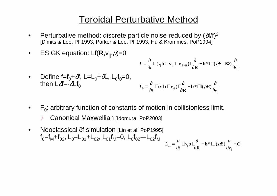
Toroidal Perturbative Method

• Perturbative method: discrete particle noise reduced by (δf/f)2

[Dimits & Lee, PF1993; Parker & Lee, PF1993; Hu & Krommes, PoP1994]

• ES GK equation: Lf(R,v||,µ)=0

• Define f=f0+δf, L=L0+δL, L0f0=0, then Lδf=-δLf0

|||| )(*)(

vBv

tL BEd ∂

∂Φ+⋅∇−∂∂⋅+++

∂∂= × µb

Rvvb

||||0 )(*)(

vBv

tL d ∂

∂⋅∇−∂∂⋅++

∂∂= µb

Rvb

• F0: arbitrary function of constants of motion in collisionless limit.

Canonical Maxwellian [Idomura, PoP2003]

• Neoclassical δf simulation [Lin et al, PoP1995] f0=fM+f02, L0=L01+L02, L01fM=0, L0f02=-L02fM

Cv

Bvt

L −∂∂⋅∇−

∂∂⋅+

∂∂=

||||01 )(* µb

Rb

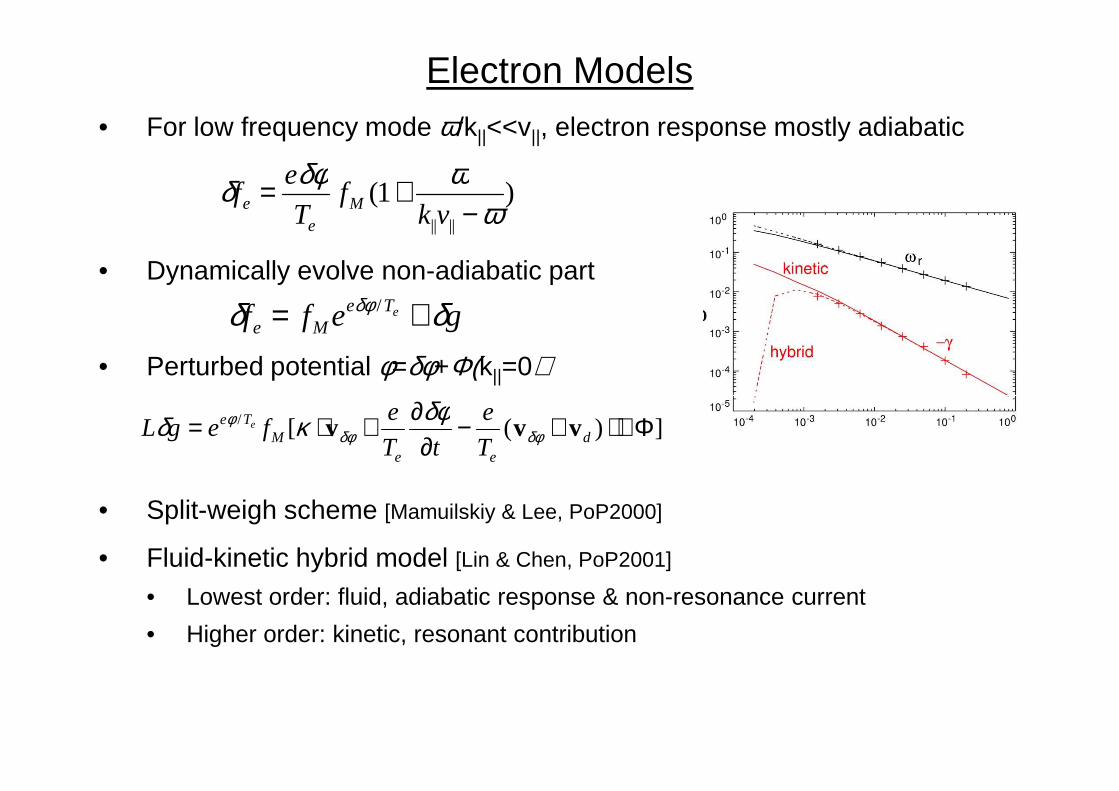
Electron Models• For low frequency mode ω/k||<<v||, electron response mostly adiabatic

• Dynamically evolve non-adiabatic part

• Perturbed potential φ=δφ+Φ(k||=0)

geff eTeMe δδ δφ += /

)1(|||| ωωδφδ−

+=vk

fT

ef M

ee

• Split-weigh scheme [Mamuilskiy & Lee, PoP2000]

• Fluid-kinetic hybrid model [Lin & Chen, PoP2001]

• Lowest order: fluid, adiabatic response & non-resonance current

• Higher order: kinetic, resonant contribution

])([/ Φ∇⋅+−∂

∂+⋅= dee

MTe

T

e

tT

efegL e vvv δφδφ

φ δφκδ

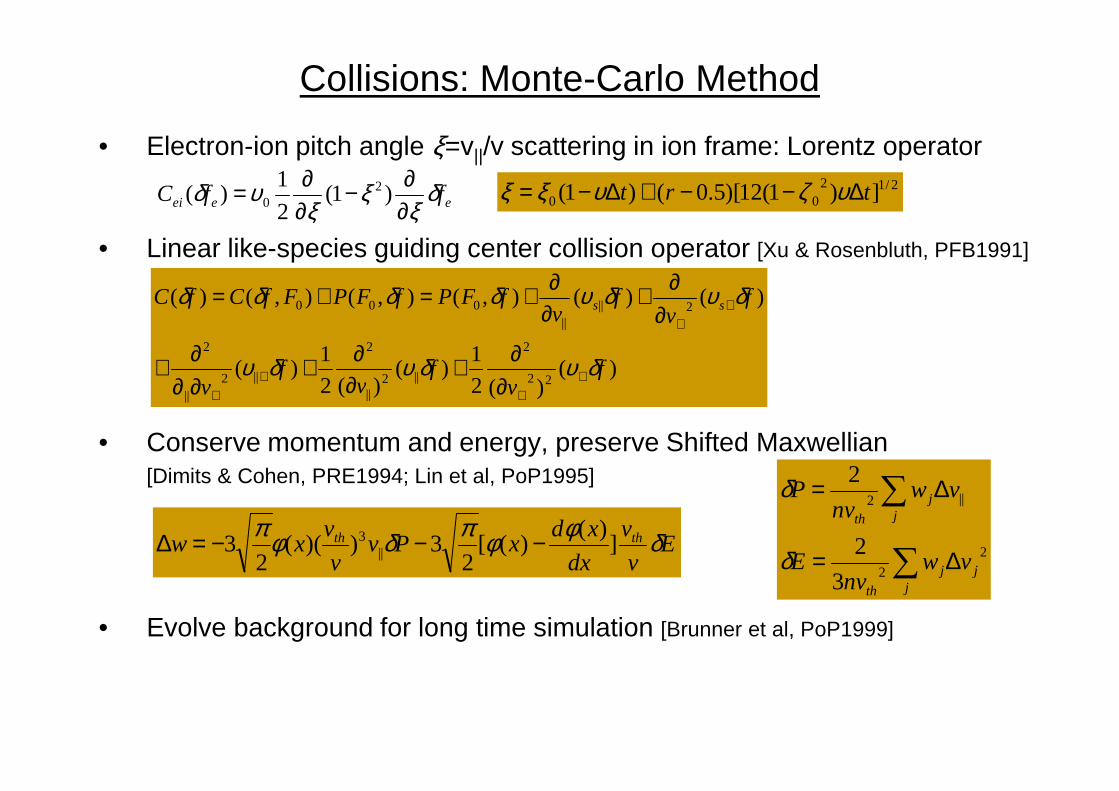
Collisions: Monte-Carlo Method

• Electron-ion pitch angle ξ=v||/v scattering in ion frame: Lorentz operator

• Linear like-species guiding center collision operator [Xu & Rosenbluth, PFB1991]

eeei ffC δξ

ξξ

υδ∂∂−

∂∂= )1(

2

1)( 2

02/12

00 ])1(12)[5.0()1( trt ∆−−+∆−= υζυξξ

)()(2

1)(

)(2

1)(

)()(),(),(),()(

22

2

||2||

2

||2||

2

2||||

000

fv

fv

fv

fv

fv

fFPfFPFfCfC ss

δυδυδυ

δυδυδδδδ

⊥⊥

⊥⊥

⊥⊥

∂∂+

∂∂+

∂∂∂+

∂∂+

∂∂+=+=

• Conserve momentum and energy, preserve Shifted Maxwellian [Dimits & Cohen, PRE1994; Lin et al, PoP1995]

• Evolve background for long time simulation [Brunner et al, PoP1999]

)(2)(2 |||| vvv ⊥⊥ ∂∂∂∂

Ev

v

dx

xdxPv

v

vxw thth δφφπδφπ

])(

)([2

3))((2

3 ||3 −−−=∆ 2

2

||2

3

2

2

jj

j

th

jj

th

vwnv

E

vwnv

P

∆=

∆=

∑

∑

δ

δ

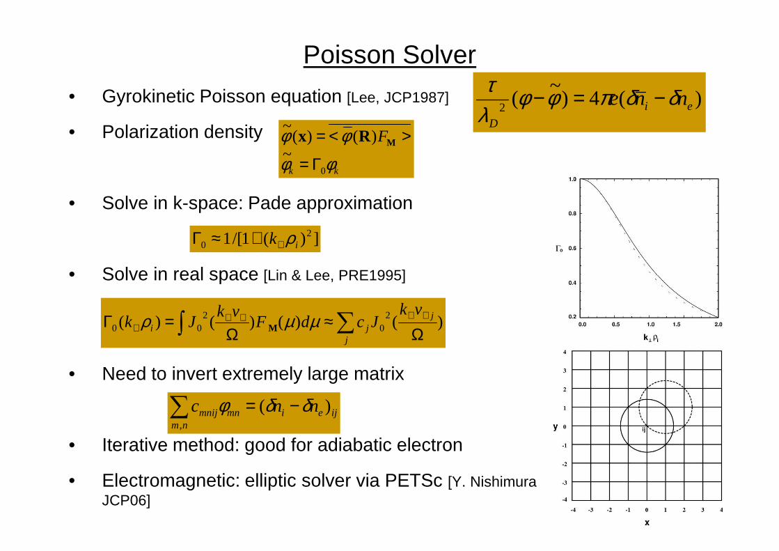
Poisson Solver

• Gyrokinetic Poisson equation [Lee, JCP1987]

• Polarization density

• Solve in k-space: Pade approximation

• Solve in real space [Lin & Lee, PRE1995]

)(4)~

(2 ei

D

nne δδπφφλτ −=−

kk

F

φφφφ

0

~)()(

~

Γ=

><= MRx

])(1/[1 20 ik ρ⊥+≈Γ

• Solve in real space [Lin & Lee, PRE1995]

• Need to invert extremely large matrix

• Iterative method: good for adiabatic electron

• Electromagnetic: elliptic solver via PETSc [Y. Nishimura JCP06]

∑∫ Ω≈

Ω=Γ ⊥⊥⊥⊥

⊥j

jji

vkJcdF

vkJk )()()()( 2

02

00 µµρ M

ijeinm

mnmnij nnc )(,

δδφ −=∑

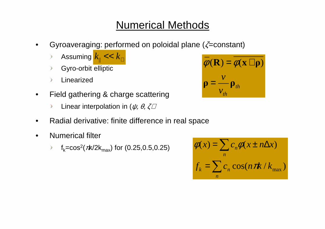
Numerical Methods

• Gyroaveraging: performed on poloidal plane (ζ=constant)

Assuming

Gyro-orbit elliptic

Linearized

• Field gathering & charge scattering

Linear interpolation in (ψ, θ, ζ)

ththv

vρρ

ρxR

=

+= )()( φφ⊥<< kk||

• Radial derivative: finite difference in real space

• Numerical filter

fk=cos2(πk/2kmax) for (0.25,0.5,0.25)

∑

∑

=

∆±=

nnk

nn

kkncf

xnxcx

)/cos(

)()(

maxπ

φφ

GTC Status and Plan

Integration of key capabilities in a single GTC version: done Kinetic electrons via fluid-kinetic hybrid electron model

Electromagnetic solver using PETSc

General geometry MHD equilibrium and plasma profiles using spline

Global field-aligned mesh using magnetic coordinates

Multi-level parallelism using mixed mode of MPI/OpenMP

Advanced I/O using ADIOS Advanced I/O using ADIOS

Plan for GTC upgrades: full-f ion simulation & neoclassical physics

GTC is part of benchmark suites for DOE OASCR, NERSC, and Cray; pioneering applications of ORNL petaflop computers (30M hours); INCITE (30M hours); SciDAC GPS, GSEP, & CPES

Key active developers: Z. Lin, I. Holod, W. Zhang, Y. Xiao (UCI), S. Klasky (ORNL), S. Ethier (PPPL). Supported by SciDAC GPS, GSEP, & CPES

Google Scholar search of “gyrokinetic gtc” returns 230+ papers; SCI citation to GTC papers 1500+

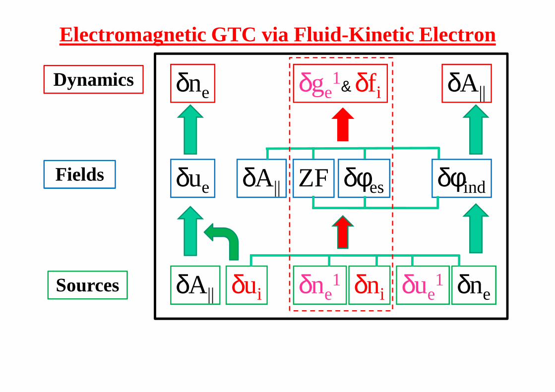
Electromagnetic GTC via Fluid-Kinetic Electron

δne δA ||

δue

δge1&δf i

δφindδφesδA || ZF

Dynamics

Fieldse

δneδne1δuiδA || δni δue

1

indes||

Sources

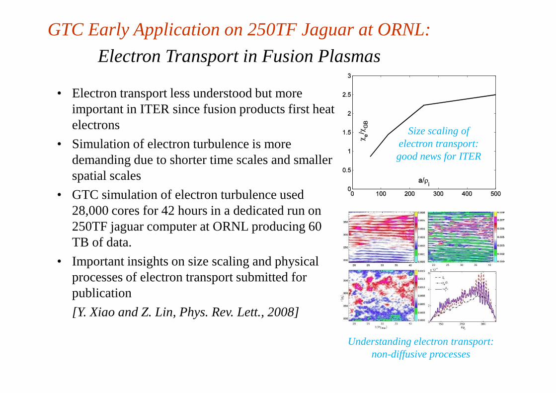
• Electron transport less understood but more important in ITER since fusion products first heat electrons

• Simulation of electron turbulence is more demanding due to shorter time scales and smaller spatial scales

• GTC simulation of electron turbulence used

GTC Early Application on 250TF Jaguar at ORNL:

Electron Transport in Fusion Plasmas

Size scaling of electron transport: good news for ITER

• GTC simulation of electron turbulence used 28,000 cores for 42 hours in a dedicated run on 250TF jaguar computer at ORNL producing 60 TB of data.

• Important insights on size scaling and physical processes of electron transport submitted for publication

[Y. Xiao and Z. Lin, Phys. Rev. Lett., 2008]

Understanding electron transport: non-diffusive processes

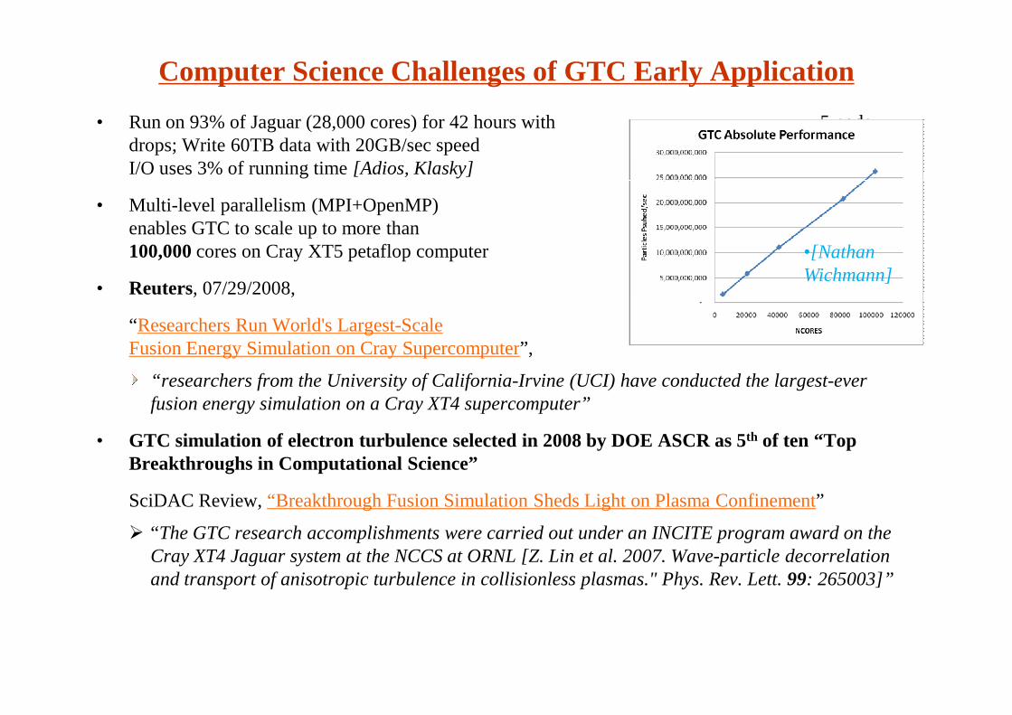
Computer Science Challenges of GTC Early Application

• Run on 93% of Jaguar (28,000 cores) for 42 hours with 5 node drops; Write 60TB data with 20GB/sec speed I/O uses 3% of running time [Adios, Klasky]

• Multi-level parallelism (MPI+OpenMP) enables GTC to scale up to more than 100,000cores on Cray XT5 petaflop computer

• Reuters, 07/29/2008,

“Researchers Run World's Largest-Scale Fusion Energy Simulation on Cray Supercomputer”,

•[Nathan Wichmann]

Fusion Energy Simulation on Cray Supercomputer”,

“researchers from the University of California-Irvine (UCI) have conducted the largest-ever fusion energy simulation on a Cray XT4 supercomputer”

• GTC simulation of electron turbulence selected in 2008 by DOE ASCR as 5th of ten “Top Breakthroughs in Computational Science”

SciDAC Review, “Breakthrough Fusion Simulation Sheds Light on Plasma Confinement”

“The GTC research accomplishments were carried out under an INCITE program award on the Cray XT4 Jaguar system at the NCCS at ORNL [Z. Lin et al. 2007. Wave-particle decorrelation and transport of anisotropic turbulence in collisionless plasmas." Phys. Rev. Lett. 99: 265003]”

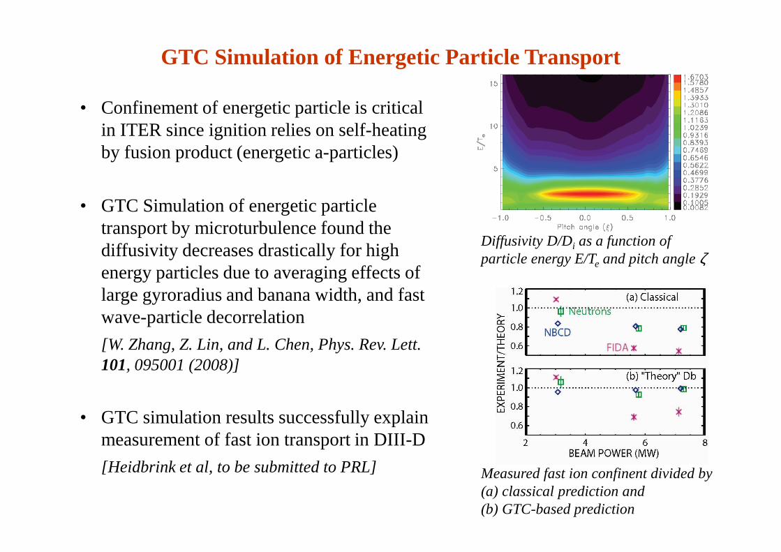
Diffusivity D/Di as a function of particle energy E/Te and pitch angle ζ

GTC Simulation of Energetic Particle Transport

• Confinement of energetic particle is critical in ITER since ignition relies on self-heating by fusion product (energetic a-particles)

• GTC Simulation of energetic particle transport by microturbulence found the diffusivity decreases drastically for high energy particles due to averaging effects of energy particles due to averaging effects of large gyroradius and banana width, and fast wave-particle decorrelation

[W. Zhang, Z. Lin, and L. Chen, Phys. Rev. Lett. 101, 095001 (2008)]

• GTC simulation results successfully explain measurement of fast ion transport in DIII-D

[Heidbrink et al, to be submitted to PRL] Measured fast ion confinent divided by (a) classical prediction and (b) GTC-based prediction

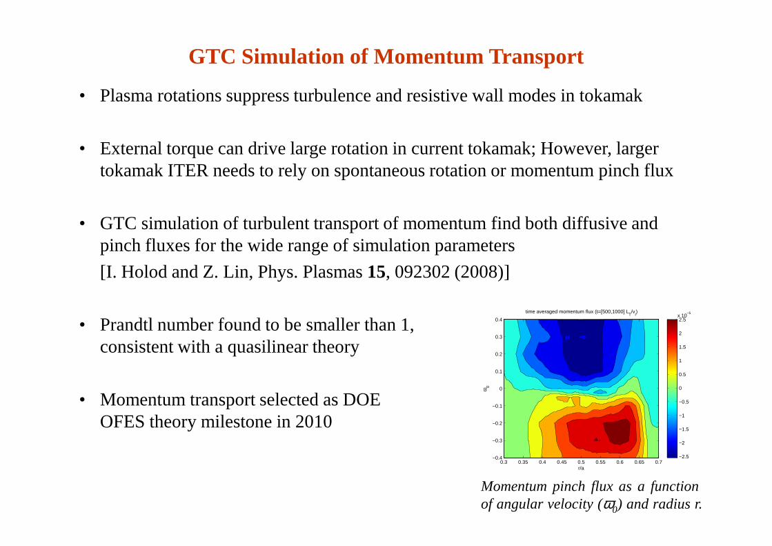
GTC Simulation of Momentum Transport

• Plasma rotations suppress turbulence and resistive wall modes in tokamak

• External torque can drive large rotation in current tokamak; However, larger tokamak ITER needs to rely on spontaneous rotation or momentum pinch flux

• GTC simulation of turbulent transport of momentum find both diffusive and pinch fluxes for the wide range of simulation parameters

[I. Holod and Z. Lin, Phys. Plasmas 15, 092302 (2008)]

time averaged momentum flux (t=[500,1000] LT/v

i)

r/a

ω0

0.3 0.35 0.4 0.45 0.5 0.55 0.6 0.65 0.7−0.4

−0.3

−0.2

−0.1

0

0.1

0.2

0.3

0.4

−2.5

−2

−1.5

−1

−0.5

0

0.5

1

1.5

2

2.5x 10

−5

Momentum pinch flux as a functionof angular velocity (ω0) and radius r.

[I. Holod and Z. Lin, Phys. Plasmas 15, 092302 (2008)]

• Prandtl number found to be smaller than 1, consistent with a quasilinear theory

• Momentum transport selected as DOE OFES theory milestone in 2010

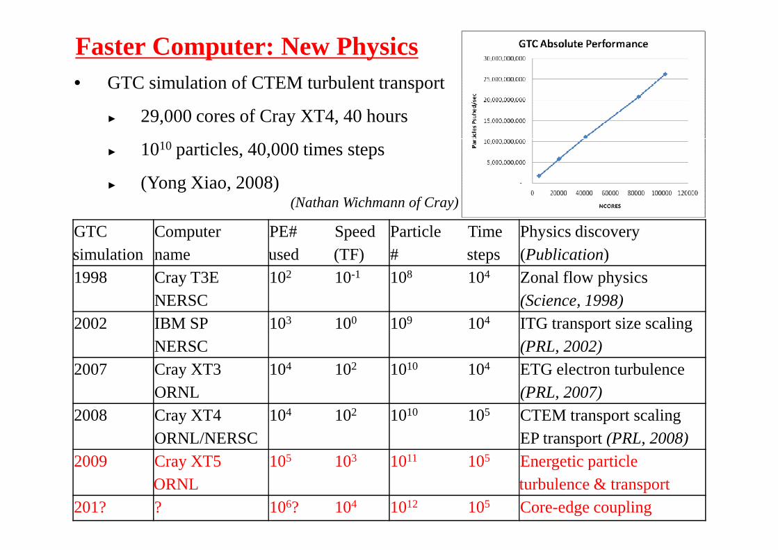
Faster Computer: New Physics

GTCsimulation

Computername

PE#used

Speed(TF)

Particle#

Timesteps

Physics discovery(Publication)

1998 CrayT3E 102 10-1 108 104 Zonalflow physics

• GTC simulation of CTEM turbulent transport

29,000 cores of Cray XT4, 40 hours

1010 particles, 40,000 times steps

(Yong Xiao, 2008)(Nathan Wichmann of Cray)

1998 CrayT3ENERSC

102 10-1 108 104 Zonalflow physics(Science, 1998)

2002 IBM SPNERSC

103 100 109 104 ITG transport size scaling(PRL, 2002)

2007 Cray XT3ORNL

104 102 1010 104 ETG electron turbulence(PRL, 2007)

2008 Cray XT4ORNL/NERSC

104 102 1010 105 CTEM transport scalingEP transport (PRL, 2008)

2009 Cray XT5 ORNL

105 103 1011 105 Energetic particle turbulence & transport

201? ? 106? 104 1012 105 Core-edge coupling

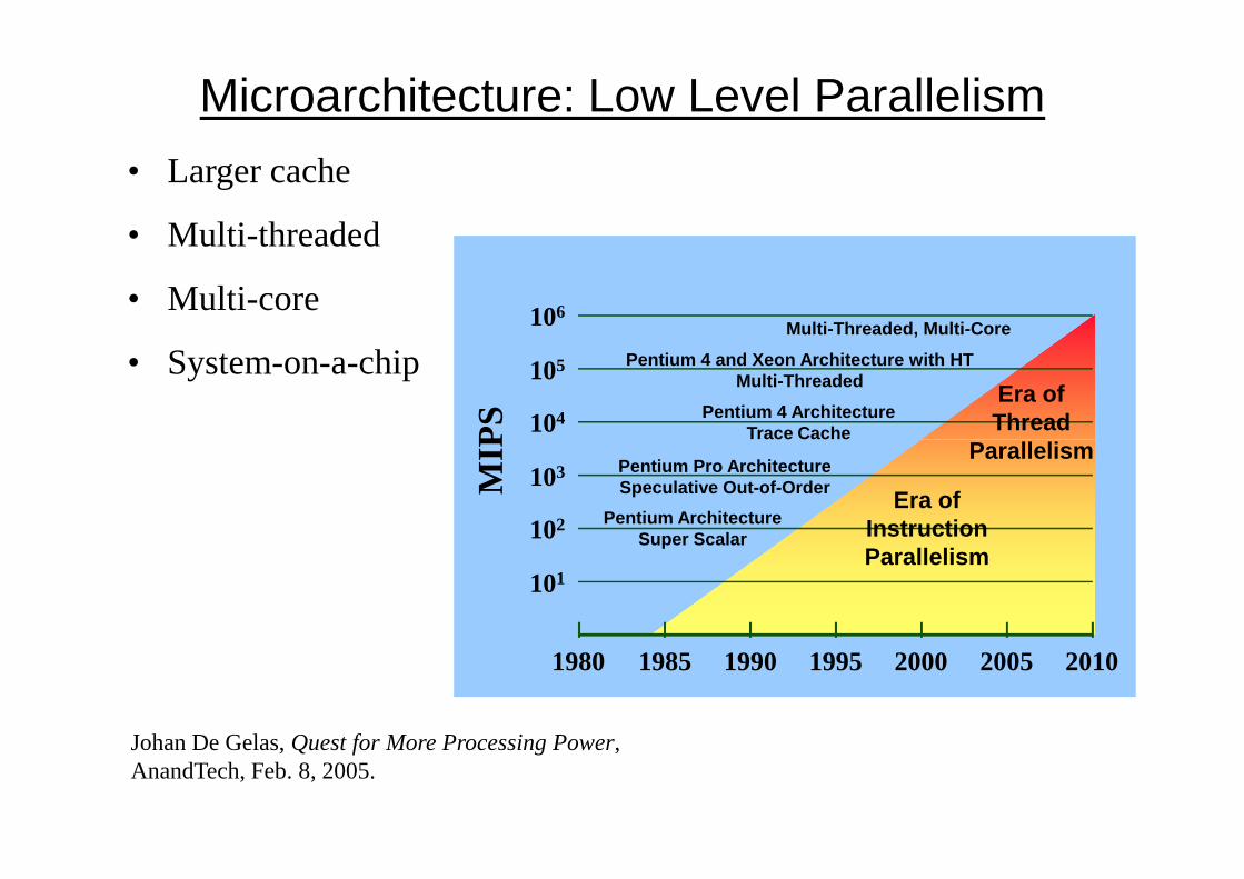
Microarchitecture: Low Level Parallelism

104

105

106

MIP

S Pentium 4 ArchitectureTrace Cache

Pentium 4 and Xeon Architecture with HTMulti-Threaded

Multi-Threaded, Multi-Core

Era ofThread

Parallelism

• Larger cache

• Multi-threaded

• Multi-core

• System-on-a-chip

Johan De Gelas, Quest for More Processing Power,AnandTech, Feb. 8, 2005.

101

102

103MIP

S

1980 1985 1990 1995 2000 2005 2010

Pentium ArchitectureSuper Scalar

Pentium Pro ArchitectureSpeculative Out-of-Order

Trace Cache

Era ofInstructionParallelism

Parallelism

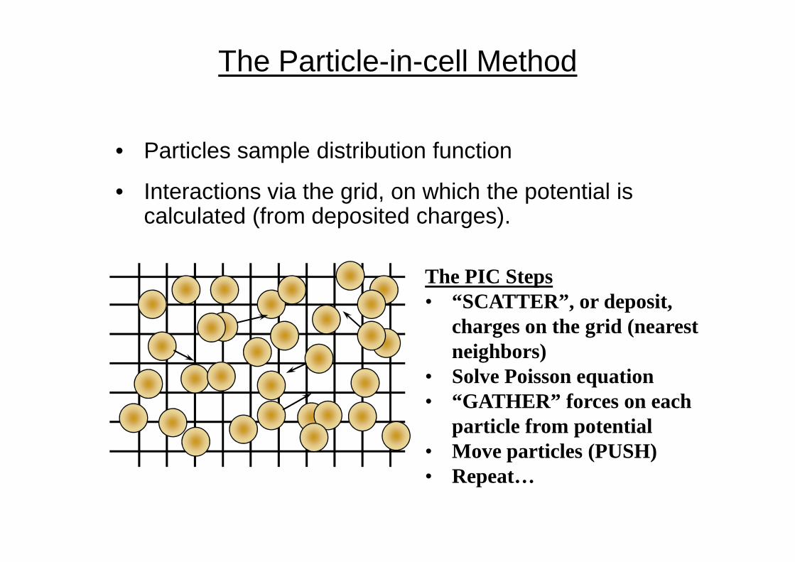
The Particle-in-cell Method

• Particles sample distribution function

• Interactions via the grid, on which the potential is calculated (from deposited charges).

The PIC StepsThe PIC Steps• “SCATTER”, or deposit,

charges on the grid (nearest neighbors)

• Solve Poisson equation• “GATHER” forces on each

particle from potential• Move particles (PUSH)• Repeat…

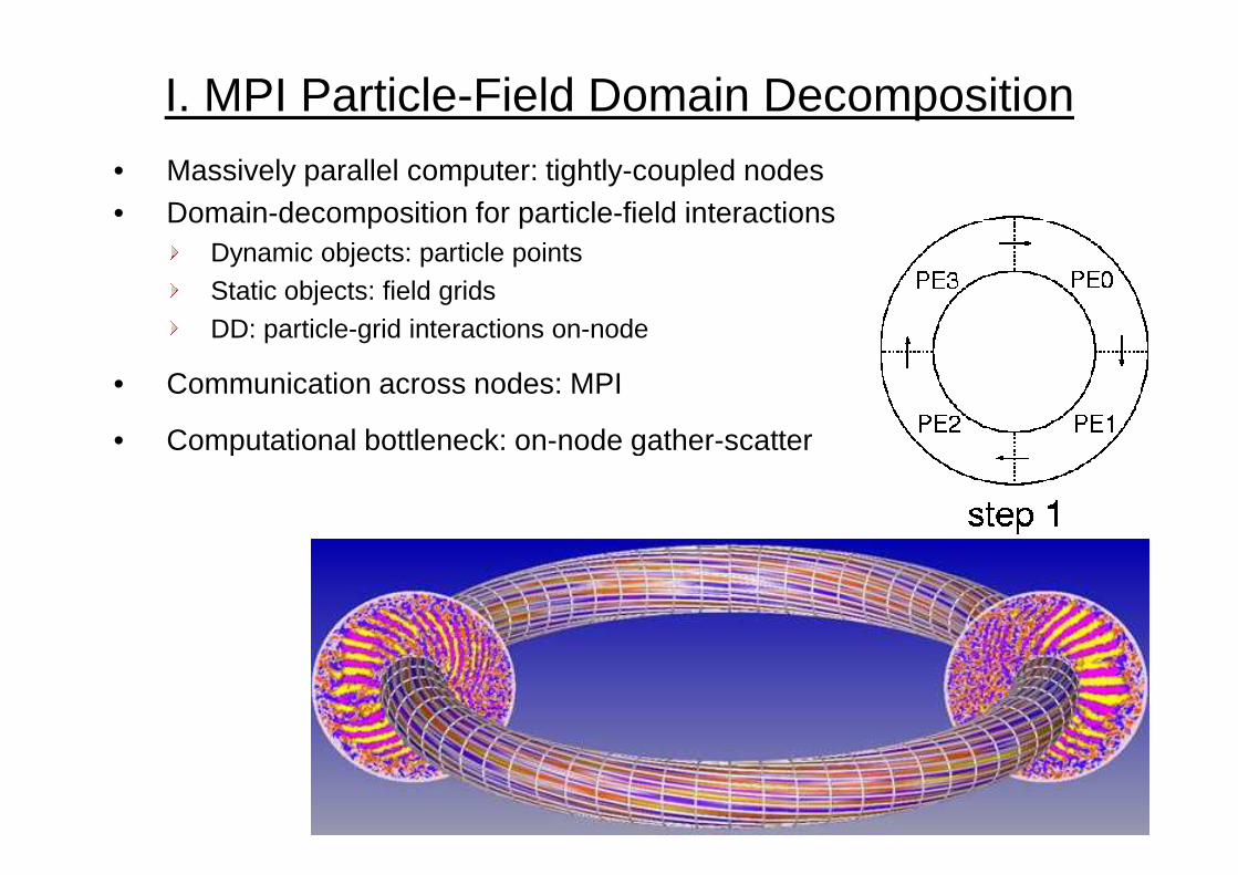
I. MPI Particle-Field Domain Decomposition

• Massively parallel computer: tightly-coupled nodes• Domain-decomposition for particle-field interactions

Dynamic objects: particle pointsStatic objects: field gridsDD: particle-grid interactions on-node

• Communication across nodes: MPI

• Computational bottleneck: on-node gather-scatter• Computational bottleneck: on-node gather-scatter

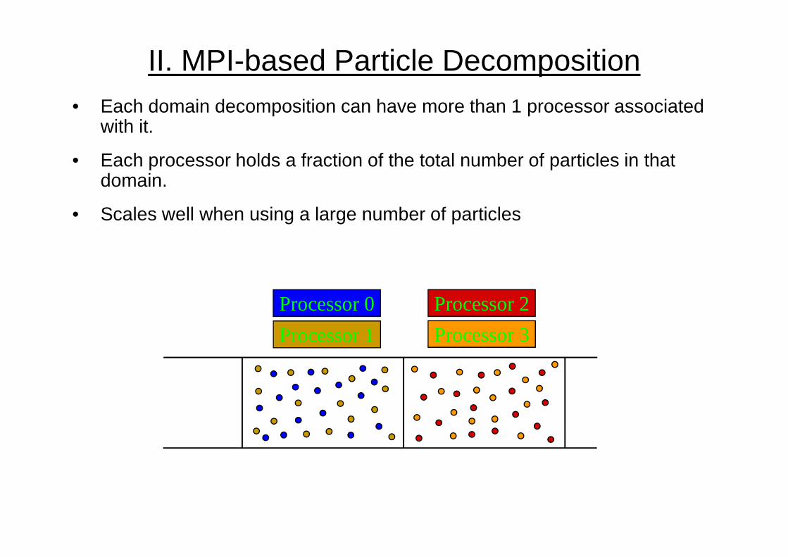
II. MPI-based Particle Decomposition• Each domain decomposition can have more than 1 processor associated

with it.

• Each processor holds a fraction of the total number of particles in that domain.

• Scales well when using a large number of particles

Processor 2

Processor 3

Processor 0

Processor 1

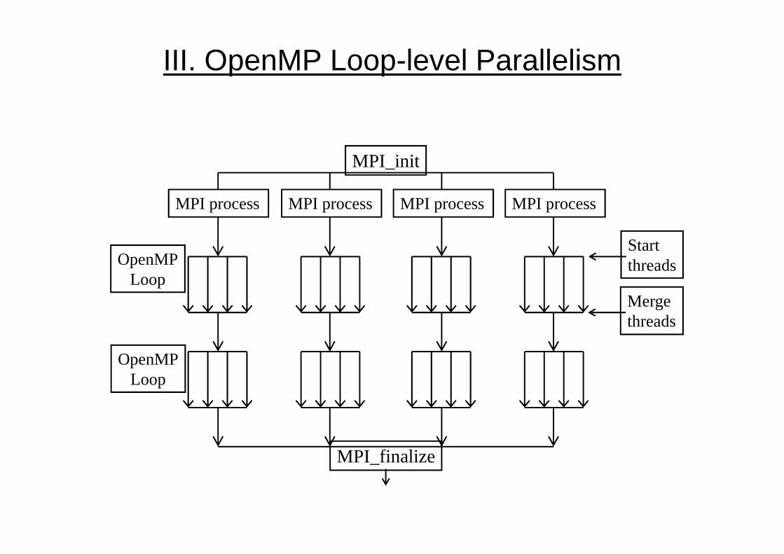
III. OpenMP Loop-level Parallelism

MPI_init

MPI process MPI process MPI process MPI process

OpenMPLoop

Startthreads

MPI_finalize

Loop

OpenMPLoop

Mergethreads

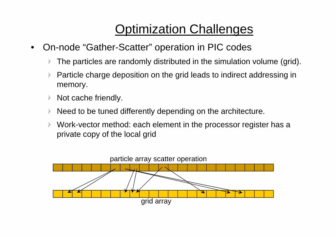
• On-node “Gather-Scatter” operation in PIC codesThe particles are randomly distributed in the simulation volume (grid).

Particle charge deposition on the grid leads to indirect addressing in memory.

Not cache friendly.

Need to be tuned differently depending on the architecture.

Optimization Challenges

Work-vector method: each element in the processor register has a private copy of the local grid

particle array scatter operation

grid array