Gravitational Lenses

[Schneider, Ehlers, & Falco, Gravitational Lenses, Springer-Verlag1992]

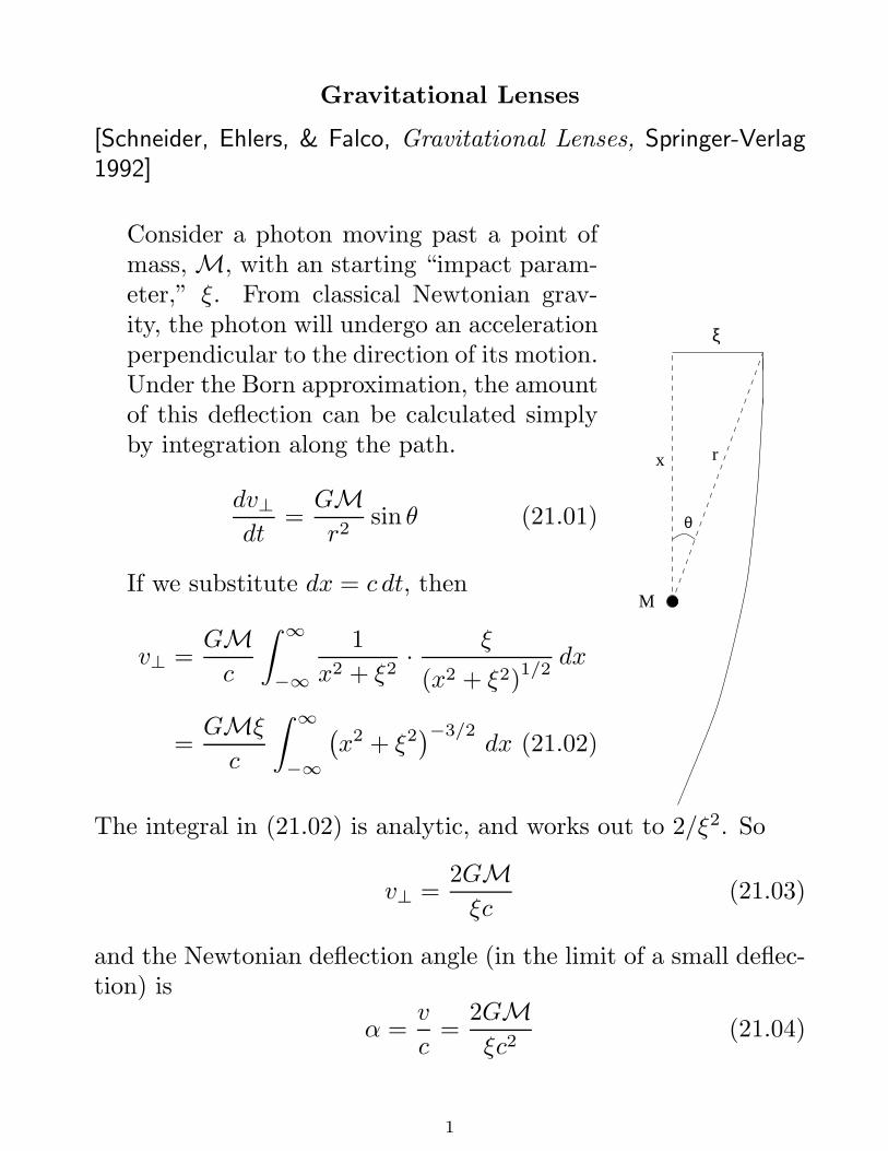
Consider a photon moving past a point ofmass, M, with an starting “impact param-eter,” ξ. From classical Newtonian grav-ity, the photon will undergo an accelerationperpendicular to the direction of its motion.Under the Born approximation, the amountof this deflection can be calculated simplyby integration along the path.

dv⊥dt

=GM

r2sin θ (21.01)

If we substitute dx = c dt, then

v⊥ =GM

c

∫ ∞

−∞

1

x2 + ξ2·

ξ

(x2 + ξ2)1/2

dx

=GMξ

c

∫ ∞

−∞

(

x2 + ξ2)−3/2

dx (21.02)

M

x r

θ

ξ

The integral in (21.02) is analytic, and works out to 2/ξ2. So

v⊥ =2GM

ξc(21.03)

and the Newtonian deflection angle (in the limit of a small deflec-tion) is

α =v

c=

2GM

ξc2(21.04)

1

In the general relativistic case, however, gravity affects both thespatial and time component of the photon’s path, so that theactual bending is twice this value. Thus, we define the angle ofdeflection, otherwise known as the Einstein angle, as

α =4GM

ξc2(21.05)

To understand the geometry of a gravitational lens, let’s first de-fine a few terms. Let

Dd = distance from the observer to the lensDs = distance from the observer to the light sourceDds = distance from the lens to the source~β = true angle between the lens and the source~θ = observed angle between the lens and the source~ξ = distance from the lens to a passing light ray~α = the Einstein angle of deflection

Note that β, θ, α, and ξ are all vectors, and calculations mustdeal with negative, as well as positive angles. For a simple point-source lens, the vectorial components of the angles make no differ-ence, but in systems where the lens is complex (i.e., several galax-ies/clusters along the line-of-sight) the deflection angles must beadded vectorially.

In practice, α, β, and θ are all very small, so small angle approx-imations can be used. Also, Dd, Ds, and Dds are all much biggerthan ξ. Thus, the deflection can be considered instantaneous (i.e.,we can use a “thin lens” approximation).

2

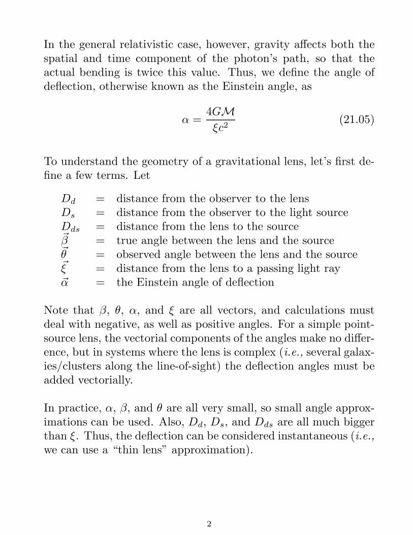
The geometry of a simple grav-itational lens system is laid outin the figure. From OSI andthe law of sines,

sin(180 − α)

Ds=

sin(θ − β)

Dds

(21.06)

Since all the angles are small,sin(θ−β) ≈ θ−β, and sin(180−α) = sinα ≈ α. So

~β = ~θ −Dds

Ds~α (21.07)

(Again, for single point lenses,the fact that the angles are vec-tors are irrelevant. For sim-plicity, I will therefore drop thevector signs for the rest of thesederivations.)

Since we have already seen that

α =4GM

ξc2(21.05)

and, from the simple geometryof small angles, θ = ξ/Dd,

M

o

S

I

D

D

Dds

s

d

β

θ

α

ξ

3

β = θ −

(

4GM

c2

Dds

DdDs

)

·1

θ(21.08)

In other words, we have a relation between β and θ. But note:for a given value of β, there is more than one value of θ thatwill satisfy the equation. This is a general theorum of lenses.For non-transparent lenses (such as the Schwarzschild lens beingconsidered) there will always be an even number of images; fortransparent lenses, there is always an odd number of images.

To simplify, let’s define the characteristic bending angle, α0, asa quantity that depends only on the mass of the lens and thedistances involved

α0 =

(

4GM

c2

Dds

DdDs

)1/2

(21.09)

so that

β = θ −α2

0

θ(21.10)

If β and θ are co-planar (as they will be for a point source lens),then (21.10) is equivalent to the quadratic equation

θ2 − βθ − α20 = 0 (21.11)

whose solution is

θ =1

2

(

β ±√

4α20 + β2

)

(21.12)

This defines the location of the gravitional lens images as a func-tion of the true position of the source with respect to the lens, β,and α0.

4

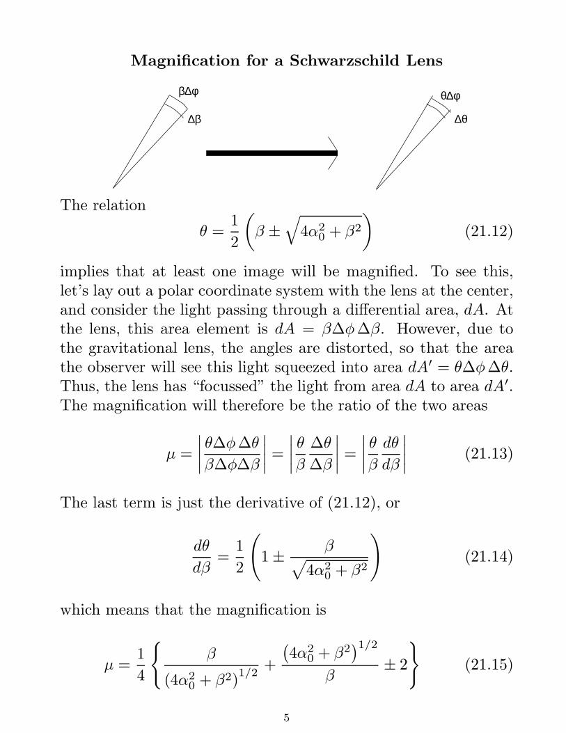
Magnification for a Schwarzschild Lens

∆β

β∆φ

∆θ

θ∆φ

The relation

θ =1

2

(

β ±√

4α20 + β2

)

(21.12)

implies that at least one image will be magnified. To see this,let’s lay out a polar coordinate system with the lens at the center,and consider the light passing through a differential area, dA. Atthe lens, this area element is dA = β∆φ∆β. However, due tothe gravitational lens, the angles are distorted, so that the areathe observer will see this light squeezed into area dA′ = θ∆φ∆θ.Thus, the lens has “focussed” the light from area dA to area dA′.The magnification will therefore be the ratio of the two areas

µ =

∣

∣

∣

∣

θ∆φ∆θ

β∆φ∆β

∣

∣

∣

∣

=

∣

∣

∣

∣

θ

β

∆θ

∆β

∣

∣

∣

∣

=

∣

∣

∣

∣

θ

β

dθ

dβ

∣

∣

∣

∣

(21.13)

The last term is just the derivative of (21.12), or

dθ

dβ=

1

2

(

1 ±β

√

4α20 + β2

)

(21.14)

which means that the magnification is

µ =1

4

β

(4α20 + β2)

1/2+

(

4α20 + β2

)1/2

β± 2

(21.15)

5

Note the limits: as β −→ ∞, µ+ −→ 1 and µ− −→ 0; in otherwords, there is no lensing. On the other hand, when β −→ 0,both µ+ and µ− go to infinity. As you can see from the curves,when β < α0, gravitational lens magnification is important.

Another feature of this magnification is that it only occurs be-cause the solid angle through which the light is flowing is beingdistorted. Moreover, nothing happens in the φ direction; only theθ coordinate is getting compressed. Consequently, the shape ofthe source will be distorted. The generalized version of (21.13) is

1

µ=

(∆ω)0ω

=

∣

∣

∣

∣

det∂β

∂θ

∣

∣

∣

∣

=As

AI

(

Dd

Ds

)2

(21.16)

where ω0 is the solid angle subtended by the source in the absenseof lensing, and the amplification is given by the determinant of theJacobian matrix. Note that this Jacobian can either be larger thanone (magnification) or smaller than one (de-magnification). It canalso be positive or negative; this gives the images orientation with

6

respect to the original source. (This is also known as the parity.)A general theorum of transparent lenses is that there is always atleast one image with positive parity and magnification.

Finally, note that the determinant in the above equation can bezero. (Or, equivalently, the magnification given in (21.15) canbe infinite. These locations are called caustics. In practice, themagnification never gets to be infinite because a) the backgroundsources have finite size, and b) if it ever does get near infinite,interference effects will become important.

There are a few other relations that should be kept in mind. Sincethe magnification of a lens is given by

µ =1

4

β

(4α20 + β2)

1/2+

(

4α20 + β2

)1/2

β± 2

(21.15)

the brightness ratio of two images is

ν =µ+

µ−

=

(

4α20 + β2

)1/2+ β

(4α20 + β2)

1/2− β

2

(21.17)

which simplies through (21.12) to

ν =µ+

µ−

=

(

θ1

θ2

)2

(21.18)

Some other convenient relations (which can be proved with somesimple algebra) are

θ1 − θ2 =(

4α20 + β2

)1/2(21.19)

β = θ1 + θ2 (21.20)

7

andθ1θ2 = −α2

0 (21.21)

(Again, remember that the angles are vector quantities, so anglessuch as θ can be positive or negative.)

8

General Scale Lengths for Lenses

It’s useful to keep in mind some of the numbers that are typicalof gravitational lens problems. Remember that the key value isα0,

α0 =

(

4GM

c2

Dds

DdDs

)1/2

(21.09)

For the MACHO project, which tries to detect stars in the LargeMagellanic Cloud (Ds = 50 kpc) that are lensed by stellar-typeobjects in the Milky Way,

α0 = 4 × 10−4

(

M

M⊙

)1/2 (

Dds

Dd

)1/2

arcsec (21.22)

In this case, the image separations θ ∼ α0 are sub-milliarcsec, soyou will never be able to resolve the two separately lensed images.But, with both images landing on top of each other, the sourcecan be (greatly) magnified.

For quasar lensing by a typical large elliptical galaxy (1012M⊙)in an Einstein-de Sitter universe,

α0 = 1.6

(

M

1012M⊙

)1/2(

zs − zd

zszd

)1/2

h1/2 arcsec (21.22)

where h is the Hubble Constant in units of 100 km/s/Mpc. Here,the typical scale-length is a little over an arcsec, so two separateimages can be resolved.

9

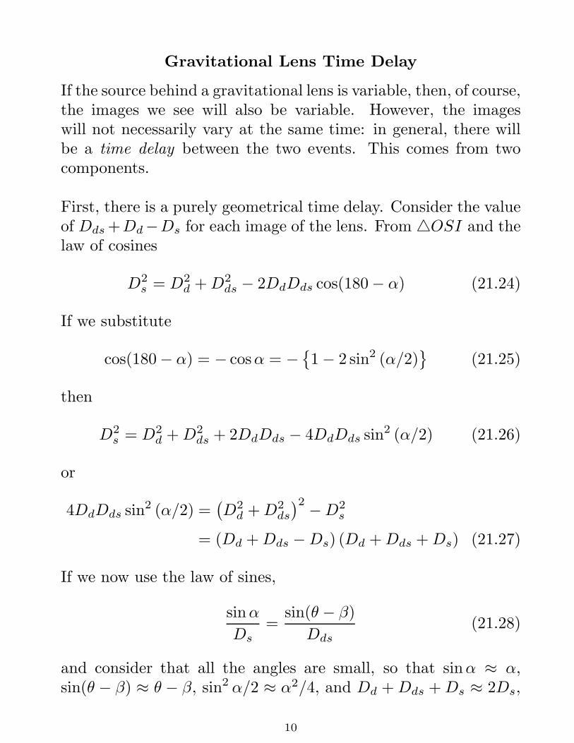
Gravitational Lens Time Delay

If the source behind a gravitational lens is variable, then, of course,the images we see will also be variable. However, the imageswill not necessarily vary at the same time: in general, there willbe a time delay between the two events. This comes from twocomponents.

First, there is a purely geometrical time delay. Consider the valueof Dds +Dd−Ds for each image of the lens. From OSI and thelaw of cosines

D2s = D2

d + D2ds − 2DdDds cos(180 − α) (21.24)

If we substitute

cos(180 − α) = − cosα = −

1 − 2 sin2 (α/2)

(21.25)

then

D2s = D2

d + D2ds + 2DdDds − 4DdDds sin2 (α/2) (21.26)

or

4DdDds sin2 (α/2) =(

D2d + D2

ds

)2− D2

s

= (Dd + Dds − Ds) (Dd + Dds + Ds) (21.27)

If we now use the law of sines,

sinα

Ds=

sin(θ − β)

Dds(21.28)

and consider that all the angles are small, so that sinα ≈ α,sin(θ − β) ≈ θ − β, sin2 α/2 ≈ α2/4, and Dd + Dds + Ds ≈ 2Ds,

10

then

Dd + Dds − Ds =4DdDds sin2

(

α2/2)

Dd + Dds + Ds

=DdDdsα

2

2Ds(21.29)

Finally, by substituting for α using (21.07), we have

Dd + Dds − Ds =DdDs

2Dds

(

~θ − ~β)2

= c∆t (21.30)

Since there are two values of ~θ, there are two values for the geo-metrical time delay. So the delay of one image with respect to theother (which is all we can observe), is

∆Tg =DdDs

2cDds

(θ1 − β)2− (θ2 − β)

2

(21.31)

If you now recall that

α0 =

(

4GM

c2

Dds

DdDs

)1/2

(21.09)

and

β = θ −α2

0

θ(21.10)

then, we can substitute these in to get

∆Tg =1

2c

4GM

c2α20

α40

θ21

−α4

0

θ22

=2GM

c3α2

0

θ22 − θ2

1

θ21θ

22

(21.32)

11

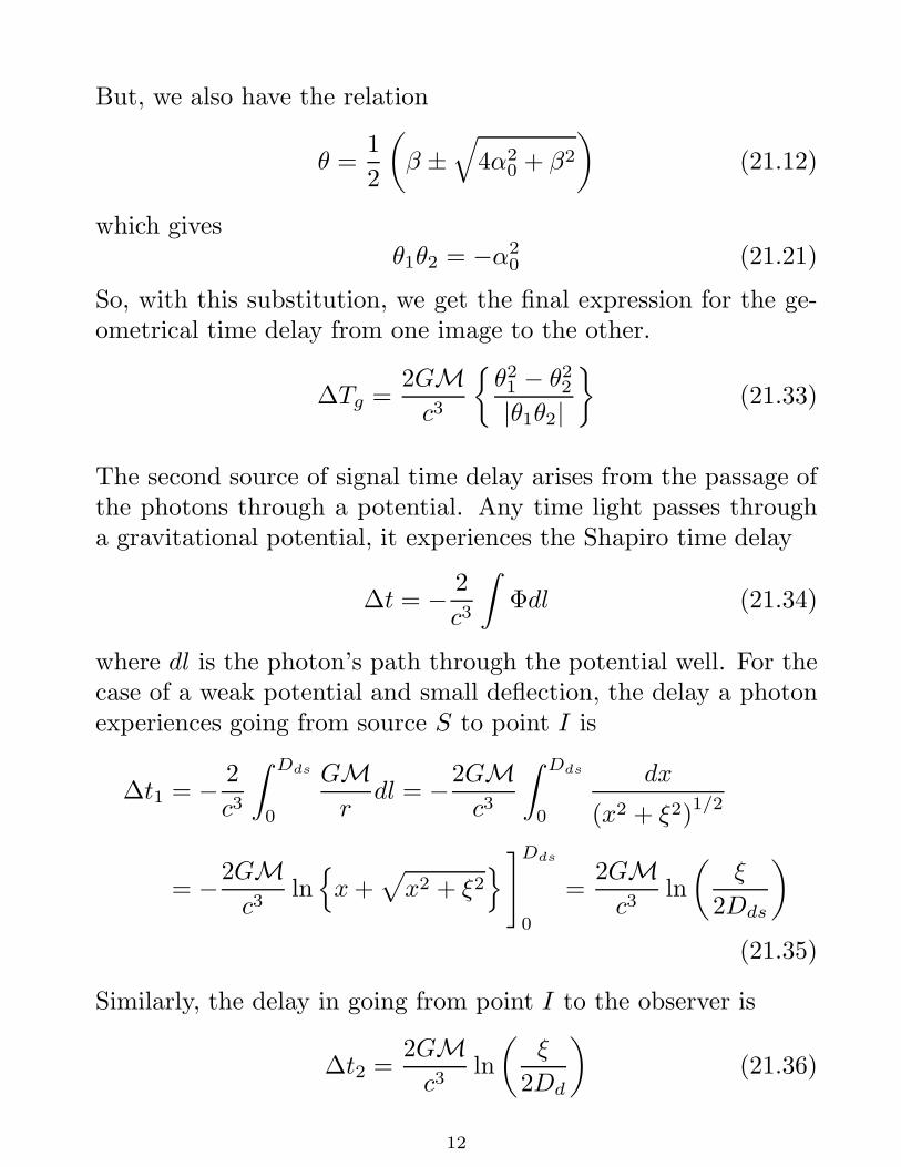
But, we also have the relation

θ =1

2

(

β ±√

4α20 + β2

)

(21.12)

which givesθ1θ2 = −α2

0 (21.21)

So, with this substitution, we get the final expression for the ge-ometrical time delay from one image to the other.

∆Tg =2GM

c3

θ21 − θ2

2

|θ1θ2|

(21.33)

The second source of signal time delay arises from the passage ofthe photons through a potential. Any time light passes througha gravitational potential, it experiences the Shapiro time delay

∆t = −2

c3

∫

Φdl (21.34)

where dl is the photon’s path through the potential well. For thecase of a weak potential and small deflection, the delay a photonexperiences going from source S to point I is

∆t1 = −2

c3

∫ Dds

0

GM

rdl = −

2GM

c3

∫ Dds

0

dx

(x2 + ξ2)1/2

= −2GM

c3ln

x +√

x2 + ξ2

]Dds

0

=2GM

c3ln

(

ξ

2Dds

)

(21.35)

Similarly, the delay in going from point I to the observer is

∆t2 =2GM

c3ln

(

ξ

2Dd

)

(21.36)

12

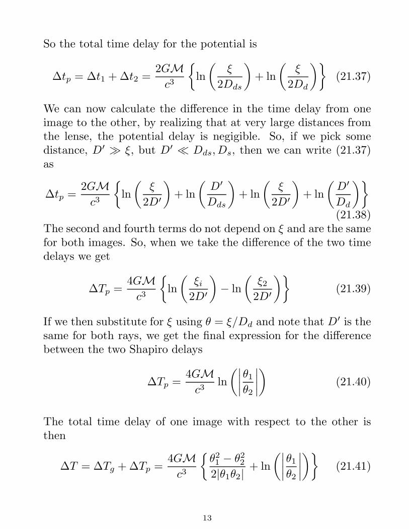
So the total time delay for the potential is

∆tp = ∆t1 + ∆t2 =2GM

c3

ln

(

ξ

2Dds

)

+ ln

(

ξ

2Dd

)

(21.37)

We can now calculate the difference in the time delay from oneimage to the other, by realizing that at very large distances fromthe lense, the potential delay is negigible. So, if we pick somedistance, D′ ≫ ξ, but D′ ≪ Dds, Ds, then we can write (21.37)as

∆tp =2GM

c3

ln

(

ξ

2D′

)

+ ln

(

D′

Dds

)

+ ln

(

ξ

2D′

)

+ ln

(

D′

Dd

)

(21.38)The second and fourth terms do not depend on ξ and are the samefor both images. So, when we take the difference of the two timedelays we get

∆Tp =4GM

c3

ln

(

ξi

2D′

)

− ln

(

ξ2

2D′

)

(21.39)

If we then substitute for ξ using θ = ξ/Dd and note that D′ is thesame for both rays, we get the final expression for the differencebetween the two Shapiro delays

∆Tp =4GM

c3ln

(∣

∣

∣

∣

θ1

θ2

∣

∣

∣

∣

)

(21.40)

The total time delay of one image with respect to the other isthen

∆T = ∆Tg + ∆Tp =4GM

c3

θ21 − θ2

2

2|θ1θ2|+ ln

(∣

∣

∣

∣

θ1

θ2

∣

∣

∣

∣

)

(21.41)

13

Note, however, that this equation neglects two important effects.

1) The universe is expanding an possibly non-Euclidean; thus, thevariables Ds, Ds, and Dds are complex functions of z, Ω0, andΛ. Specifically, Dd and Ds are angular distances, and Dds is theangular size distance of the source as seen by an observed at the

redshift of the lens.

2) Cosmological lenses are not point sources. The best lenses are el-liptical galaxies (which are fairly concentrated collections of stars),but these galaxies are located inside of clusters. So real lenses in-clude the effects of both the galaxy and the cluster (which, ofcourse, add vectorially).

14

The Uses of Gravitational Lenses

Gravitational lenses are extremely interesting for four reasons.

1) Because the magnification properties of lenses depend on the massof the lensing object, microlensing experiments, such as OGLEand MACHO (which monitor millions of stars in the GalacticBulge and the Large Magellanic Cloud), can probe the propertiesof halo stars (and other objects) that are two faint to see. Infact, by studying the light curve of a gravitational microlens, onecan deduce not only the mass of the intervening lens (with someassumption about the lens’ distance), but also whether the lensis a single star or something else. Microlensing experiments havemeasured light curves that must be due to binary-star lenses, and,in a few cases, have detected planets around stars. (In theory,the amplitude of the microlens event does not depend on mass,so even Earth-size (and lunar-size) bodies can be detected. Inpractice, while the amplitude of the event is independent of mass,the duration of the event is proportional to mass, so, in order todetect planet-sized bodies, excellent and continuous time coverageis needed.

2) Because of their high magnification, gravitational lenses can beused to observe high-redshift galaxies that would normally bemuch too faint to observe otherwise. There is a slight problemwith this, in that the image of the galaxy is usually distorted(spread out) over many pixels (into an arc). However, if the lightcan be collected, you can use it to study a representative sampleof normal (not exceptionally bright) high-redshift galaxies. Thisproperty has been used to detect and measure galaxies as distantas z > 7.

15

3) Because the time delay of a gravitational lens depends on dis-tance, these objects can be used to measure the Hubble Constant.Unfortunately, this method has two major drawbacks. First, thetime delay depends not only on the distance to the lens, but itsmass as well. This mass is not known a priori: for a typical el-liptical galaxy lens, one must try to infer the lens mass from thevelocity dispersion of its stars. Second, the geometry of the lensis usually complicated. Elliptical galaxies are in clusters, and thecluster’s mass will also contribute to the time delay. One musttherefore measure the velocity dispersion of the galaxies in thecluster in order to determine the cluster’s mass (while, of course,hoping that the cluster is virialized, and that none of the objectsyou are measuring are foreground or background objects). More-over, for distant sources, it is likely that the calculations will befurther complicated by the presence of multiple lenses along theline-of-sight.

4) All clusters (and halos) along a line-of-sight cause some (small)amount of magnification. Moreover, because the mapping of thesource into the image plane is asymmetric, each event will causethe background images to be slightly distorted. Thus, it is possibleto obtain a census of galaxies (and clusters) just be looking forsmall distortions in the shapes of distant galaxies. By seeing howthis (weak) signal changes with position on the sky, one can deriveinformation about galaxy clusters throughout the universe, andconstrain the evolution of heirachical clustering (which dependssensitively on Λ).

16

General Comments on Real Lenses

As we have seen, the bending angle for a lens is

α =4GM

ξc2(21.05)

This implies that as ξ −→ 0, the bending angle (and magnifica-tion) becomes infinite. This doesn’t happen with cosmologicallenses, because the lenses are never point masses. Instead, themass is distributed, i.e., M(ξ), which goes to zero as ξ goes tozero. So the equations do not diverge.

In practice, the gravitational deflection due to a galaxy’s clusteris almost as important as that of the galaxy itself. Consequently,one must model the lens with a galaxy plus cluster potential, andthis breaks the symmetry of the problem. Hence, the equation tosolve is

~α =

∫

4G∑ ~ξ′

c2

~ξ − ~ξ′

|~ξ − ~ξ′|2dξ′ (21.42)

In other words, the bending angle is the vector sum of the gravi-tational deflections caused by all the mass in the two-dimensionalcluster.

17

The best lenses are massive and compact objects. For cosmo-logical lenses, this means elliptical galaxies. (They are the mostcompact of all galaxies.) Consequently, even though the majorityof galaxies are spirals, it is generally reasonable to assume thatall gravitatational lenses are caused by ellipticals. Ideally, to usea gravitational lens as a cosmological probe, you would like

1) Optical identifications for both the lens and the source. (Occa-sionally, the lens is too faint to be studied.)

2) A measured velocity dispersion for the lens (to estimate its mass).

3) A variable source (to measure the time delay for the two images).

4) An angular separation between the two images of 1′′ < ∆θ < 2′′.If the separation is any smaller, it is hard to resolve the images;if the separation is any larger, then the cluster’s mass begins todominate the problem. Also, recall that

∆T = ∆Tg + ∆Tp =4GM

c3

θ21 − θ2

2

2|θ1θ2|+ ln

(∣

∣

∣

∣

θ1

θ2

∣

∣

∣

∣

)

(21.41)

hence the gravitational time delay ∆T ∝ ∆θ2. Small separationskeep the time delay manageable. (For instance, the lens 0957+561has a separation of 6′′, and a time delay of between 1 and 2 years.)

5) VLBI radio structure, so that the shape of the images can be usedto constrain the mass distribution of the lens.

6) Multiple images to constrain the geometry. Four images are betterthan two, and an Einstein ring is best.

18

Statistical Microlensing

Consider a Schwartzschild (point source) lens at redshift z in frontof a source at redshift zs. The magnification of the two images isgiven by

µ =1

4

β

(4α20 + β2)

1/2+

(

4α20 + β2

)1/2

β± 2

(21.15)

If the two images are unresolved (i.e., the case of microlensing),then the total magnification is

µT = µ+ + µ− =1

2

2α20 + β2

β (4α20 + β2)

1/2

(21.43)

With a little bit of math, this equation can be inverted to give theangle β, which yields a total magnification of µT

β2 = 2α20

µT

(µ2T − 1)

1/2− 1

(21.44)

The cross-sectional area for a magnification of greater than µT tooccur is therefore

σ(µT , z, zs) = πβ2 (21.45)

This means that at redshift zs, any object located in an area of

σ(µT , z, zs) = πD2sβ

2 (21.46)

will be microlensed.

19

Now, let’s calculate the probability that a source at redshift zs willbe microlensed. To begin, let’s assume that the density of lensesis given by η. (Since the best lenses are elliptical galaxies, youconsider η to be the density of elliptical galaxies.) For simplicity,let’s also assume that η does not evolve with time (there are asmany elliptical galaxies today as there were at redshift z), andthat each lens has identical lensing properties (same mass, samemass concentration, etc.)

If η0 is the density of lenses today, then the density of lenses atredshift z is given by

η(z) = η0(1 + z)3 (21.47)

and the total number of lenses between z and z + dz is

dN(z) = ηdV = η0(1 + z)3dV (21.48)

where dV is the cosmological volume element. (For Euclideanspace, this would normally just be 4πr2dr, but because of theuniversal expansion and the possible non-flat geometry of space,the actual expression is a complicated function of z, Ω0, and Λ.)

Now if the density of lenses is small enough so that the probabilityof two lenses overlapping each other is negligible, then the totalarea at redshift zs that is microlensed up to at least a magnifica-tion of µT is just the sum of the cross-sections of all the lenses,i.e.,

σt(zs) =

∫

σ(µT , z, zs)dN =

∫ zs

0

σ(µT , z, zs)η0(1 + z)3dV

(21.49)

20

The probability of a microlens is then just this area, normalizedto the total surface area of the universe at redshift zs

At = 4πD2ang (21.50)

where D2ang is the angular-size distance of redshift z.

This “statistical microlensing” is extremely important. In fact,with typical numbers for the space density of elliptical galaxylenses, you find that by z = 2, half the objects in the sky aremagnified by at least 10%!

21