Gravimetry, Relativity, and theGlobal Navigation Satellite Systems

Albert TarantolaInstitut de Physique du Globe de Paris

Ludek KlimesCharles University, Prague

Jose Maria Pozo and Bartolome CollObservatoire de Paris

1

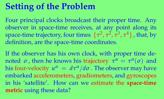
Setting of the ProblemFour principal clocks broadcast their proper time. Anyobserver in space-time receives, at any point along itsspace-time trajectory, four times τ2, τ2, τ3, τ4 , that, bydefinition, are the space-time coordinates.

If the observer has his own clock, with proper time de-noted σ , then he knows his trajectory τα = τα(σ) andhis four-velocity uα = dτα/dσ . The observer may haveembarked accelerometers, gradiometers, and gyroscopesin his ‘satellite’. How can we estimate the space-timemetric using these data?

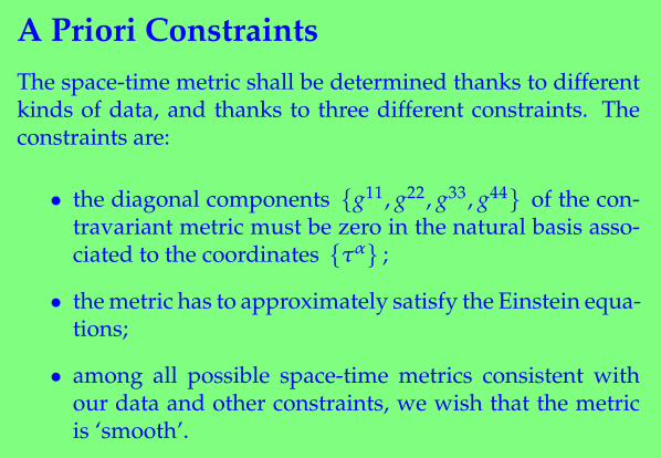
A Priori ConstraintsThe space-time metric shall be determined thanks to differentkinds of data, and thanks to three different constraints. Theconstraints are:

• the diagonal components g11, g22, g33, g44 of the con-travariant metric must be zero in the natural basis asso-ciated to the coordinates τα ;

• the metric has to approximately satisfy the Einstein equa-tions;

• among all possible space-time metrics consistent withour data and other constraints, we wish that the metricis ‘smooth’.

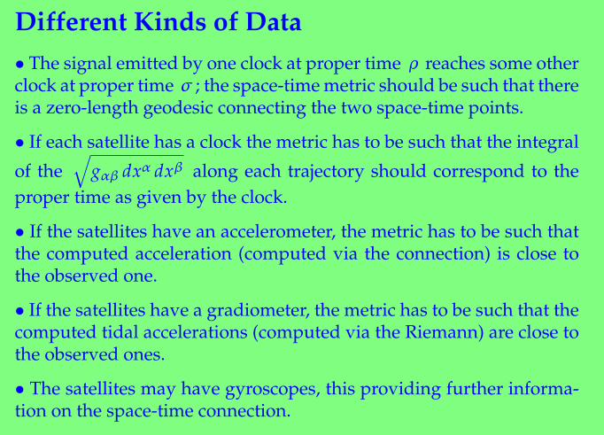
Different Kinds of Data• The signal emitted by one clock at proper time ρ reaches some otherclock at proper time σ ; the space-time metric should be such that thereis a zero-length geodesic connecting the two space-time points.

• If each satellite has a clock the metric has to be such that the integralof the

√gαβ dxα dxβ along each trajectory should correspond to the

proper time as given by the clock.

• If the satellites have an accelerometer, the metric has to be such thatthe computed acceleration (computed via the connection) is close tothe observed one.

• If the satellites have a gradiometer, the metric has to be such that thecomputed tidal accelerations (computed via the Riemann) are close tothe observed ones.

• The satellites may have gyroscopes, this providing further informa-tion on the space-time connection.

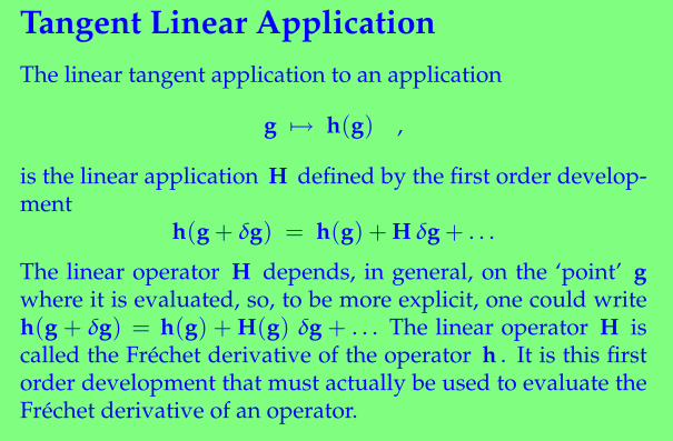
Tangent Linear ApplicationThe linear tangent application to an application

g !→ h(g) ,

is the linear application H defined by the first order develop-ment

h(g + δg) = h(g) + H δg + . . .

The linear operator H depends, in general, on the ‘point’ gwhere it is evaluated, so, to be more explicit, one could writeh(g + δg) = h(g) + H(g) δg + . . . The linear operator H iscalled the Frechet derivative of the operator h . It is this firstorder development that must actually be used to evaluate theFrechet derivative of an operator.

Transpose of a Linear OperatorLet L be a linear operator mapping a linear space A into alinear space B . Let A∗ and B∗ the respective dual spaces,and 〈 · , · 〉A and 〈 · , · 〉B the respective duality products.

The transpose of L is the linear operator mapping B∗ into A∗such that for any a ∈ A and any b∗ ∈ B∗ ,

〈 b∗ , L a 〉B = 〈 Lt b∗ , a 〉A .

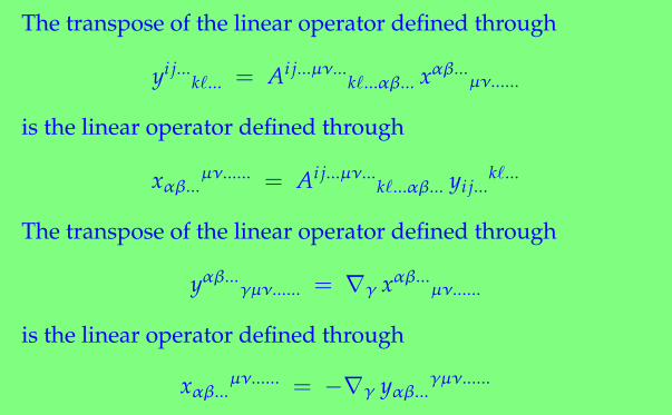
The transpose of the linear operator defined through

yi j...k!... = Ai j...µν...

k!...αβ... xαβ...µν......

is the linear operator defined through

xαβ...µν...... = Ai j...µν...

k!...αβ... yi j...k!...

The transpose of the linear operator defined through

yαβ...γµν...... = ∇γ xαβ...

µν......

is the linear operator defined through

xαβ...µν...... = −∇γ yαβ...

γµν......

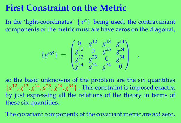
First Constraint on the MetricIn the ‘light-coordinates’ τα being used, the contravariantcomponents of the metric must are have zeros on the diagonal,

gαβ =

0 g12 g13 g14

g12 0 g23 g24

g13 g23 0 g34

g14 g24 g34 0

,

so the basic unknowns of the problem are the six quantitiesg12, g13, g14, g23, g24, g34 . This constraint is imposed exactly,by just expressing all the relations of the theory in terms ofthese six quantities.

The covariant components of the covariant metric are not zero.

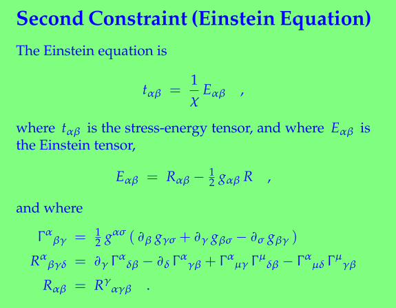
Second Constraint (Einstein Equation)The Einstein equation is

tαβ =1χ

Eαβ ,

where tαβ is the stress-energy tensor, and where Eαβ isthe Einstein tensor,

Eαβ = Rαβ − 12 gαβ R ,

and where

Γαβγ = 1

2 gασ ( ∂β gγσ + ∂γ gβσ − ∂σ gβγ )

Rαβγδ = ∂γ Γα

δβ − ∂δ Γαγβ + Γα

µγ Γµδβ − Γα

µδ Γµγβ

Rαβ = Rγαγβ .

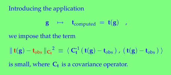
Introducing the application

g !→ tcomputed = t(g) ,

we impose that the term

‖ t(g)− tobs ‖Ct2 ≡ 〈 C-1

t ( t(g)− tobs ) , ( t(g)− tobs ) 〉is small, where Ct is a covariance operator.

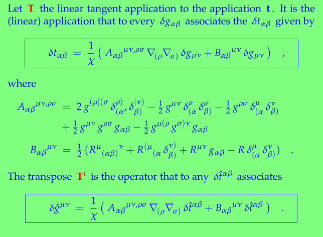
Let T the linear tangent application to the application t . It is the(linear) application that to every δgαβ associates the δtαβ given by

δtαβ =1χ

(Aαβ

µν,ρσ ∇(ρ∇σ) δgµν + Bαβµν δgµν

),

where

Aαβµν,ρσ = 2 g(µ|(σ

δρ)(α , δ|ν)

β) − 12 gµν δρ

(α δσβ) − 1

2 gρσ δµ(α δν

β)

+ 12 gµν gρσ gαβ − 1

2 gµ(ρ gσ)ν gαβ

Bαβµν = 1

2 (Rµ(αβ)

ν + R(µ(α δ

ν)β) + Rµν gαβ − R δµ

(α δνβ)) .

The transpose Tt is the operator that to any δtαβ associates

δgµν =1χ

(Aαβ

µν,ρσ ∇(ρ∇σ) δtαβ + Bαβµν δtαβ

).

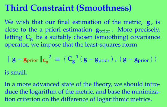
Third Constraint (Smoothness)We wish that our final estimation of the metric, g , isclose to the a priori estimation gprior . More precisely,letting Cg be a suitably chosen (smoothing) covarianceoperator, we impose that the least-squares norm

‖ g − gprior ‖Cg2 ≡ 〈 C−1

g ( g − gprior ) , ( g − gprior ) 〉is small.

In a more advanced state of the theory, we should intro-duce the logarithm of the metric, and base the minimiza-tion criterion on the difference of logarithmic metrics.

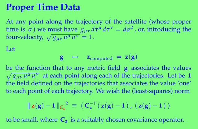
Proper Time DataAt any point along the trajectory of the satellite (whose propertime is σ ) we must have gµν dτµ dτν = dσ2 , or, introducing thefour-velocity,

√gµν uµ uν = 1 .

Letg "→ zcomputed = z(g)

be the function that to any metric field g associates the values√gµν uµ uν at each point along each of the trajectories. Let be 1

the field defined on the trajectories that associates the value ‘one’to each point of each trajectory. We wish the (least-squares) norm

‖ z(g)− 1 ‖Cz2 ≡ 〈 C−1

z ( z(g)− 1 ) , ( z(g)− 1 ) 〉to be small, where Cz is a suitably chosen covariance operator.

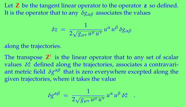
Let Z be the tangent linear operator to the operator z so defined.It is the operator that to any δgαβ associates the values

δz =1

2√

gµν uµ uνuα uβ δgαβ

along the trajectories.

The transpose Zt is the linear operator that to any set of scalarvalues δz defined along the trajectories, associates a contravari-ant metric field δgαβ that is zero everywhere excepted along thegiven trajectories, where it takes the value

δgαβ =1

2√

gµν uµ uνuα uβ δz .

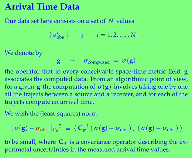
Arrival Time DataOur data set here consists on a set of N values

σ iobs ; i = 1, 2, . . . , N .

We denote byg !→ σ computed = σ(g)

the operator that to every conceivable space-time metric field gassociates the computed data. From an algorithmic point of view,for a given g the computation of σ(g) involves taking one by oneall the trajects between a source and a receiver, and for each of thetrajects compute an arrival time.

We wish the (least-squares) norm

‖σ(g)−σobs ‖Cσ2 ≡ 〈 C−1

σ (σ(g)−σobs ) , (σ(g)−σobs ) 〉to be small, where Cσ is a covariance operator describing the ex-perimetal uncertainties in the measured arrival time values.

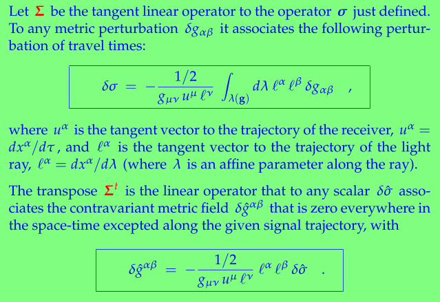
Let Σ be the tangent linear operator to the operator σ just defined.To any metric perturbation δgαβ it associates the following pertur-bation of travel times:

δσ = − 1/2gµν uµ !ν

∫λ(g)

dλ !α !β δgαβ ,

where uα is the tangent vector to the trajectory of the receiver, uα =dxα/dτ , and !α is the tangent vector to the trajectory of the lightray, !α = dxα/dλ (where λ is an affine parameter along the ray).

The transpose Σt is the linear operator that to any scalar δσ asso-ciates the contravariant metric field δgαβ that is zero everywhere inthe space-time excepted along the given signal trajectory, with

δgαβ = − 1/2gµν uµ !ν

!α !β δσ .

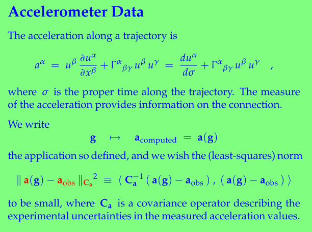
Accelerometer DataThe acceleration along a trajectory is

aα = uβ ∂uα

∂xβ+ Γα

βγ uβ uγ =duα

dσ+ Γα

βγ uβ uγ ,

where σ is the proper time along the trajectory. The measureof the acceleration provides information on the connection.

We writeg !→ acomputed = a(g)

the application so defined, and we wish the (least-squares) norm

‖ a(g)− aobs ‖Ca2 ≡ 〈 C−1

a ( a(g)− aobs ) , ( a(g)− aobs ) 〉to be small, where Ca is a covariance operator describing theexperimental uncertainties in the measured acceleration values.

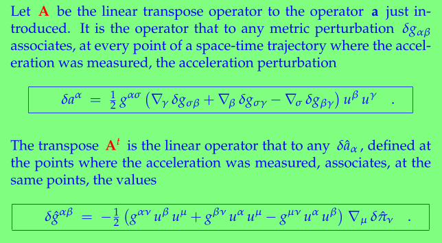
Let A be the linear transpose operator to the operator a just in-troduced. It is the operator that to any metric perturbation δgαβ

associates, at every point of a space-time trajectory where the accel-eration was measured, the acceleration perturbation

δaα = 12 gασ

(∇γ δgσβ +∇β δgσγ −∇σ δgβγ

)uβ uγ .

The transpose At is the linear operator that to any δaα , defined atthe points where the acceleration was measured, associates, at thesame points, the values

δgαβ = − 12(

gαν uβ uµ + gβν uα uµ − gµν uα uβ) ∇µ δπν .

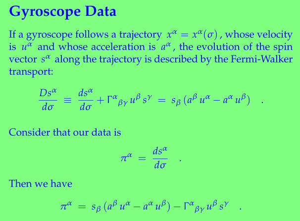
Gyroscope DataIf a gyroscope follows a trajectory xα = xα(σ) , whose velocityis uα and whose acceleration is aα , the evolution of the spinvector sα along the trajectory is described by the Fermi-Walkertransport:

Dsα

dσ≡ dsα

dσ+ Γα

βγ uβ sγ = sβ (aβ uα − aα uβ) .

Consider that our data is

πα =dsα

dσ.

Then we have

πα = sβ (aβ uα − aα uβ)− Γαβγ uβ sγ .

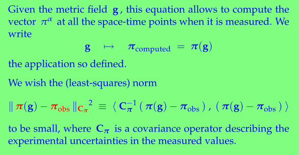
Given the metric field g , this equation allows to compute thevector πα at all the space-time points when it is measured. Wewrite

g !→ π computed = π(g)

the application so defined.

We wish the (least-squares) norm

‖π(g)− πobs ‖Cπ2 ≡ 〈 C−1

π ( π(g)− πobs ) , ( π(g)− πobs ) 〉to be small, where Cπ is a covariance operator describing theexperimental uncertainties in the measured values.

RemarkOf course, one may not wish to measure the evolution ofthe spin vector to provide information on the connection,but to ‘test’ general relativity, as in the Gravity Probe Bexperiment. From the viewpoint of the present work, thedetection of any inconsistency in the data would put rel-ativity theory in jeopardy.

Let Π be the linear tangent application to the application π justintroduced. To any metric perturbation δgαβ it associates

δπα = − 12 gασ

(∇γ δgσβ +∇β δgσγ −∇σ δgβγ

)uβ σγ .

The transpose Πt is the linear operator that to any δπα associates

δgαβ = − 14(

gαν (uβ σµ + uµ σβ) + gβν (uα σµ + uµ σα)− gµν (uα σβ + uβ σα)

) ∇µ δπν .

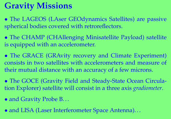
Gravity Missions• The LAGEOS (LAser GEOdynamics Satellites) are passivespherical bodies covered with retroreflectors.

• The CHAMP (CHAllenging Minisatellite Payload) satelliteis equipped with an accelerometer.

• The GRACE (GRAvity recovery and Climate Experiment)consists in two satellites with accelerometers and measure oftheir mutual distance with an accuracy of a few microns.

• The GOCE (Gravity Field and Steady-State Ocean Circula-tion Explorer) satellite will consist in a three axis gradiometer.

• and Gravity Probe B. . .

• and LISA (Laser Interferometer Space Antenna). . .

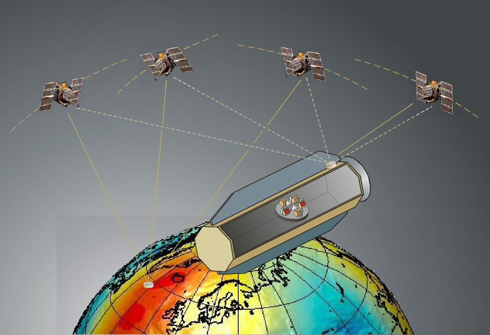
GOCE Gradiometer

GOCE will employ a three-axis electrostatic gravity gradiometerthat will allow gravity gradients to be measured in all spatial di-rections. The measured signal is the difference in gravitationalacceleration at the test-mass location inside the spacecraft causedby gravity anomalies from attracting masses of the Earth. Exploit-ing these differential measurements for all three spatial axes hasthe advantage that all disturbing forces acting uniformly on thespacecraft (i.e. drag, thrusters resulting in linear or angular accel-erations) can be compensated for. The length of the baseline foran accelerometer pair is 50 cm.

geod

esic

not g

eode

sic

u wδv

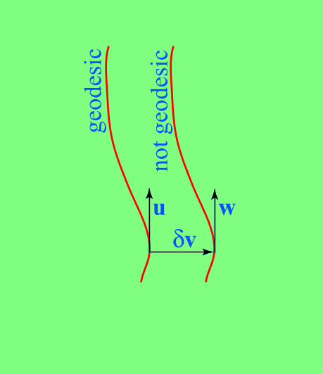
Gradiometer DataAt first order in δvα , δaα = Rα

µνρ uµ uρ δvν . As the three vectorsaα , uα , and δvα are known, we obtain information on the compo-nents of the Riemann tensor. We drop the δ for the vector δvα , andwe write ωα instead of δaα :

ωα = Rαµνρ uµ uρ vν .

Given a metric field g , the theoretical values of the tidal accelera-tion are detoted ωcomputed , and we write

g !→ ωcomputed = ω(g) .

The gradiometer provides the ‘observed acceleration’ ωobs , withobservational uncertainties represented by a covariance operatorCω . We wish the following norm to be small:

‖ω(g)−ωobs ‖Cω2 ≡ 〈 C−1

ω (ω(g)−ωobs ) , (ω(g)−ωobs ) 〉 .

Let Ω be the linear tangent operator to the operator ω just intro-duced. To any metric perturbation δgαβ it associates the perturbation

δωα = δRαβγδ uβ uδ vγ

of the tidal acceleration, where

δRαβγδ = 2∇[γΩα

δ]β ,

with Ωαβγ = gασΩσβγ , and Ωαβγ = 1

2 (∇γδgαβ +∇βδgαγ−∇αδgβγ) .

The transpose Ωt is the linear operator that to any δωα associates

δgαβ = vµ uν (uα∇µνδωβ + uβ∇µνδωα)+(uα vβ + uβ vα) uµ∇µνδων

−uµ uν (vα∇µνδωβ + vβ∇µνδωα

−2 uα uβ vµ∇µνδων .

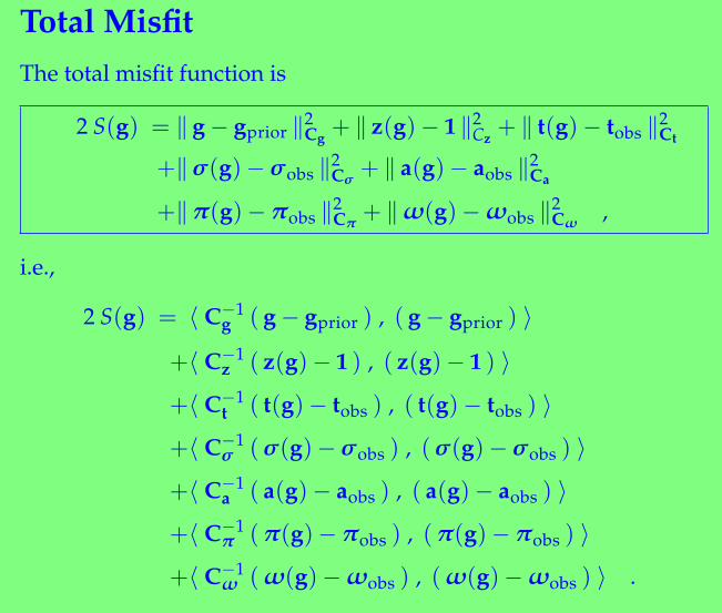
Total MisfitThe total misfit function is

2 S(g) = ‖ g − gprior ‖2Cg

+ ‖ z(g)− 1 ‖2Cz

+ ‖ t(g)− tobs ‖2Ct

+‖σ(g)−σobs ‖2Cσ

+ ‖ a(g)− aobs ‖2Ca

+‖π(g)− πobs ‖2Cπ

+ ‖ω(g)−ωobs ‖2Cω

,

i.e.,

2 S(g) = 〈 C−1g ( g − gprior ) , ( g − gprior ) 〉

+〈 C−1z ( z(g)− 1 ) , ( z(g)− 1 ) 〉

+〈 C−1t ( t(g)− tobs ) , ( t(g)− tobs ) 〉

+〈 C−1σ (σ(g)−σobs ) , (σ(g)−σobs ) 〉

+〈 C−1a ( a(g)− aobs ) , ( a(g)− aobs ) 〉

+〈 C−1π ( π(g)− πobs ) , ( π(g)− πobs ) 〉

+〈 C−1ω (ω(g)−ωobs ) , (ω(g)−ωobs ) 〉 .

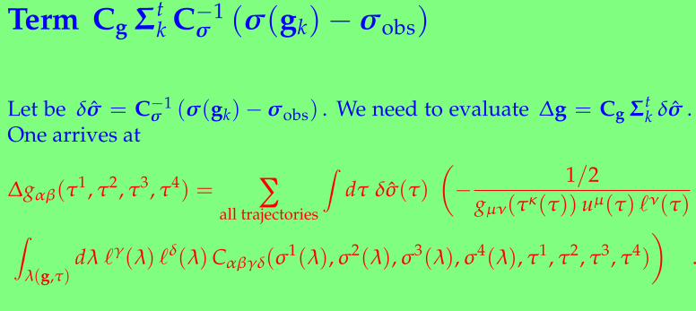
Term Cg Σtk C−1

σ (σ(gk)−σobs)

Let be δσ = C−1σ (σ(gk)−σobs) . We need to evaluate ∆g = Cg Σt

k δσ .One arrives at

∆gαβ(τ1, τ2, τ3, τ4) = ∑all trajectories

∫dτ δσ(τ)

(− 1/2

gµν(τκ(τ)) uµ(τ) !ν(τ)∫λ(g,τ)

dλ !γ(λ) !δ(λ) Cαβγδ(σ1(λ),σ2(λ),σ3(λ),σ4(λ), τ1, τ2, τ3, τ4))

.

BibliographyAshby, N., 2002, Relativity and the global positioning system, Physics Today, 55 (5), May 2002, pp.

41–47.

Cerveny, V., 2002, Fermat’s variational principle for anisotropic inhomogeneous media, Stud. geophys.geod., vol. 46, pp. 567–588, online at http://sw3d.mff.cuni.cz .

Coll, B., and Morales, J.A., 1992, 199 causal classes of space-time frames, International Journal of Theo-retical Physics, Vol. 31, No. 6, pp. 1045–1062.

Coll, B., 2002, A principal positioning system for the Earth, JSR 2002, eds. N. Capitaine and M. Stavin-schi, Pub. Observatoire de Paris, pp. 34–38.

Coll, B. and Tarantola, A., 2003, Galactic positioning system; physical relativistic coordinates for theSolar system and its surroundings, eds. A. Finkelstein and N. Capitaine, JSR 2003, Pub. St. Peters-bourg Observatory, pp. 333-334.

Hernandez-Pastora, J.L., Martın, J., and Ruiz, E., 2001, On gyroscope precession, arXiv:gr-qc/0009062.

Klimes, L., 2002, Second-order and higher-order perturbations of travel time in isotropic and anisotro-pic media, Stud. geophys. geod., vol. 46, pp. 213–248, online at http://sw3d.mff.cuni.cz .

Papapetrou, A., 1951, Spinning test-particles in general relativity (I), Proceedings of the Royal Societyof London. A209, pp. 248–258

Tarantola, A., 2004, Inverse problem theory and methods for model parameter estimation, SIAM.

Taylor, A.E., and Lay, D.C., 1980, Introduction to functional analysis, Wiley.

Weinberg, S., 1972, Gravitation and Cosmology, Wiley.

The following slides are not to be shown:they are kept in reserve

just in the case there are questions.

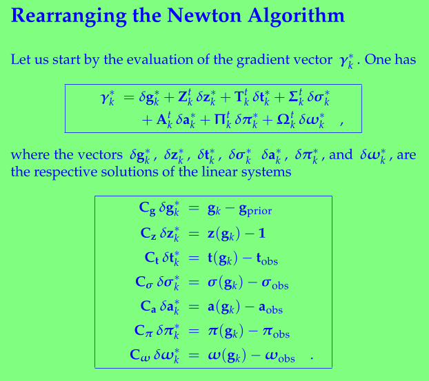
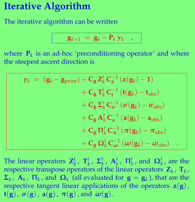
Rearranging the Newton Algorithm

Let us start by the evaluation of the gradient vector γ∗k . One has

γ∗k = δg∗k + Ztk δz∗k + Tt

k δt∗k + Σtk δσ∗

k

+ Atk δa∗k + Πt

k δπ∗k + Ωt

k δω∗k ,

where the vectors δg∗k , δz∗k , δt∗k , δσ∗k δa∗k , δπ∗

k , and δω∗k , are

the respective solutions of the linear systems

Cg δg∗k = gk − gprior

Cz δz∗k = z(gk)− 1

Ct δt∗k = t(gk)− tobs

Cσ δσ∗k = σ(gk)−σobs

Ca δa∗k = a(gk)− aobs

Cπ δπ∗k = π(gk)− πobs

Cω δω∗k = ω(gk)−ωobs .

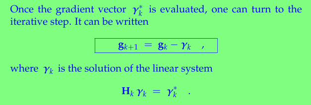
Once the gradient vector γ∗k is evaluated, one can turn to theiterative step. It can be written

gk+1 = gk −γk ,

where γk is the solution of the linear system

Hk γk = γ∗k .

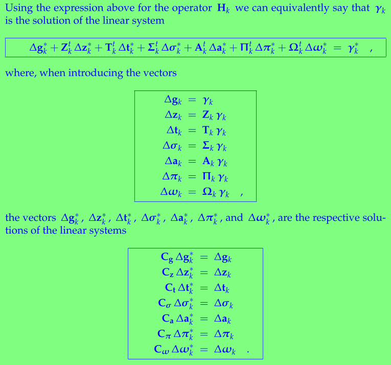
Using the expression above for the operator Hk we can equivalently say that γkis the solution of the linear system

∆g∗k + Zt

k ∆z∗k + Ttk ∆t∗k + Σt

k ∆σ∗k + At

k ∆a∗k + Πtk ∆π∗

k + Ωtk ∆ω∗

k = γ∗k ,

where, when introducing the vectors

∆gk = γk

∆zk = Zk γk

∆tk = Tk γk

∆σ k = Σk γk

∆ak = Ak γk

∆π k = Πk γk

∆ωk = Ωk γk ,

the vectors ∆g∗k , ∆z∗k , ∆t∗k , ∆σ∗

k , ∆a∗k , ∆π∗k , and ∆ω∗

k , are the respective solu-tions of the linear systems

Cg ∆g∗k = ∆gk

Cz ∆z∗k = ∆zk

Ct ∆t∗k = ∆tk

Cσ ∆σ∗k = ∆σ k

Ca ∆a∗k = ∆ak

Cπ ∆π∗k = ∆π k

Cω ∆ω∗k = ∆ωk .