1

Ground Penetrating Radar Theory and Applications

I. L. Al-QadiS. Lahouar

Presentation Overview• Background

– Nondestructive Testing– GPR Systems– Electromagnetic Theory – GPR Data Analysis

• GPR Applications– Flexible Pavements– Rigid Pavements– Rail Road

Introduction• US transportation infrastructure is deteriorating:

• 2005 ASCE Report card for American Transportation Infrastructure gave an overall grade of “D” – estimated $1.3 trillion investment needed for improvements

• Transportation agencies are shifting efforts from building new to assessing and rehabilitating existing structures

2

What is NDE?Non-destructive evaluation

Detect defects, internal distresses, measure dimensions, etc. w/o damaging the material

X-ray radiograph

• Ultrasonic waves• X-ray/ CAT scans• RADAR scanning• Thermal imaging• etc

What Are Waves?Propagation of a disturbance through a medium

(mass is not transported in propagation direction)

Direction of Travelof Wave Front

Excitation

Direction of Particle Disturbance

Important parameters: wavelength (λ), period (Τ) and frequency (f)

Ultrasonic Testing (UT)Flaw detection: wave echoes from air-filled defects such as cracks and voids

crack

wavepath

wavesource

Time

Signal amplitude

Time

Signal amplitude

Back surface echoes

crack echoes

3

Ultrasonic Pulse Velocity (UPV)

www.cnsfarnell.co.uk

d

Vp = d/t

t

Vp related to in-place material strength or presence of internal voiding and cracking (Frequency 20-200MHz)

Crack No Crack

Approach Illustration

Impact Echo Principle (ASTM C1383)

Reflected waves set up a resonance condition having a characteristic frequency (like a bell)

4

Concrete Element Inspection

2- and 3-D maps of backscatter intensity (courtesy of BAM)

• Ground Penetrating Radar (GPR):special kind of RADAR

• GPR usage:1. Detect buried targets2. Estimate their depths

• GPR applications:– Geophysics: estimate structure of earth sediments– Archeology: locate buried archeological structures– Safety tool: locate landmines– Civil Engineering: evaluate performance of civil

structures (buildings, bridges, pavements…)

GPR Applications

GPR History• Early 1900’s: RADAR Principle Was Used

to Detect Airborne Objects• Hulsenberg (1926): Detection of Buried

Objects• Austria (1929): Depth of Glacier• Late 1950’s: US Air force plane crashed

in Greenland because of wrong altitude from Radar

⇒ Ability of Radar to See Into Subsurface

5

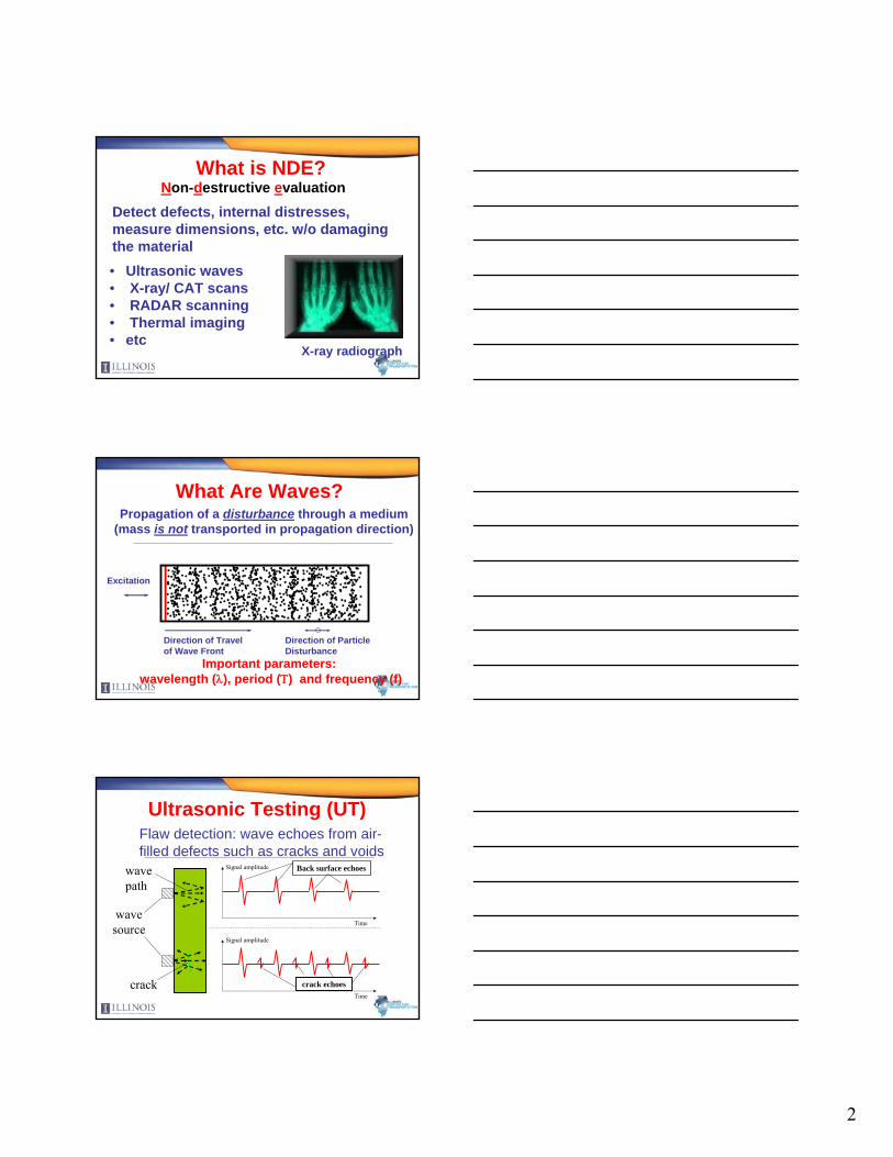
GPR History• 1960’s: Moon Surface Characterization by

NASA– Ground Probing Radar Systems Were Used in

Geological Applications• Vietnam War: “Combat Radar” Was Used to

Locate Mines, Tunnels, and Bunkers• 1970’s: Locating Sewer Lines and Cables,

Measuring Ice Thickness, Profiling Bottom of Lakes and Rivers

• 1980’s-now: Different Applications Related to Pavements and Bridge Decks

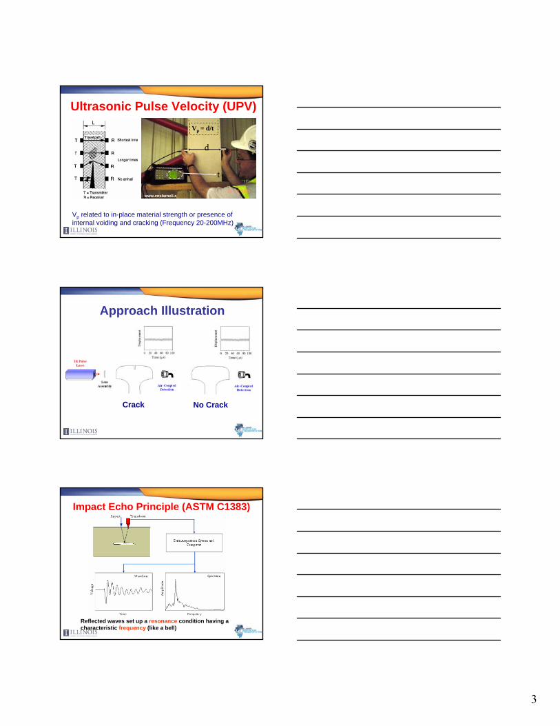
EM Properties of MaterialsInteraction of a Material with Applied Electric (E) and Magnetic (H) Fields:

– Polarization– Conductivity– Magnetic Permeability – Permittivity/ Dielectric Constant

"'rrr jεεε −=

Polarization• Electronic

Polarization:

• Ionic Polarization:

• Molecular Polarization:

• Interfacial Polarization:

++

--

---- --

------ --

++

E = 0 E ≠ 0

++--++ ++--

++E = 0 E ≠ 0

++--

++

++

--++++

--++

++--

++E = 0 E ≠ 0

------ ++--++++

++++---- ++ ++ ++ ++ ++++++

-- -- -- -- -- --E = 0 E ≠ 0

6

DIELECTRIC PROPERTIES OF CONCRETE

0.00

50.00

100.00

150.00

0.001 0.010 0.100 1.000 10.000

Frequency (GHz)

Com

plex

Die

lect

ric C

onst

ant

Parallel Plate Capacitor Coaxial T. Line TEM Antenna

Real Part

Loss Component

Typical Dielectric Constant Values

3-5Dry Sand

5-40Clays5-30Silts20-30Saturated Sand

4-6Granite5-9Limestone

3-10HMA3-18Concrete81Water1Air

Dielectric ConstantMaterial

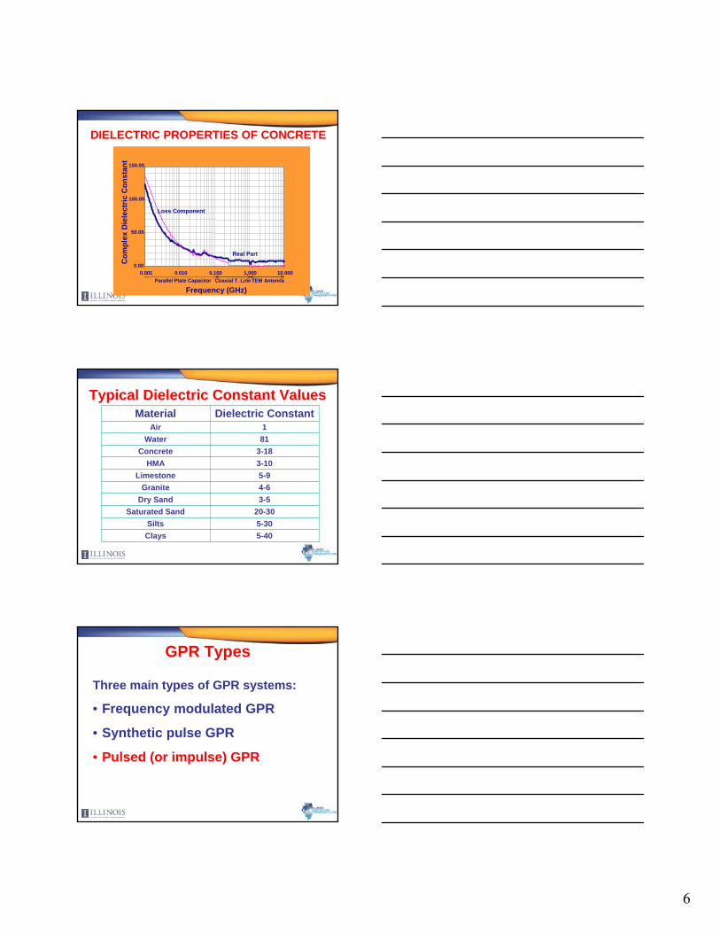
GPR Types

Three main types of GPR systems:

• Frequency modulated GPR

• Synthetic pulse GPR

• Pulsed (or impulse) GPR

7

Frequency Modulated GPR• Change frequency of

transmitted signal linearly between two limits

• Frequency difference (transmitted - reflected) proportional to the layer depth

Time

f1

f2

Freq

uenc

y

Transmitted Layer 1

Layer 2

fd1

fd2td1

td2

Synthetic Pulse GPR• Change frequency of transmitted signal

between two limits in discrete steps• Amplitude and phase of reflected signal at

each frequency step are recorded• Reflected signal reconstructed in the time

domain using an IFFT algorithm

Pulsed or Impulse GPR

• Most common type of GPR systems

• Transmitted signal is a short pulse (1 ns or less)

• Principle: Transmit a short pulse and record the reflected pulses from layer interfaces

1ns

8

GPR Antennas• Ground-coupled: the antenna is in

contact with the ground surface• Air-coupled: the antenna is 0.5m

above surface• Monostatic: one antenna used as Tx

and Rx• Bistatic: one antenna is used for Tx

and another one for Rx

GPR: How does it work?

Layer 1

Layer 2

Control Unit

Transceiver

Antenna DMI

Reflection & TransmissionAt normal incidence:• Reflection coefficient:

• Transmission coefficient:21

21

12

12

rr

rr

ηηηηγ

εεεε

+

−=

+−

=

21

1

21

2 22

rr

r

ηηητ

εεε

+=

+=

x

z

yεr 1

εr 2

EiHi

βi Er

βr

Hr

Et

βt

Ht

Incident Reflected

Transmitted

9

EM Scattering• EM scattering: occurs when there is a

discontinuity in the dielectric properties of a medium

• For pavements a discontinuity can be:– Layer interface – Distress within the layer

• At a discontinuity: – Reflection – Transmission

Typical GPR Response (scan)

HMA

Base

Subgrade

t1

t2

A1

A2

-8000

-6000

-4000

-2000 0

2000

4000

6000

8000

10000

12000

02

46

810

1214

16

Tim

e (ns)

Amplitude

HM

AB

aseSubgrade

A0

Typical Raw GPR Data

HMA

Base

Subgrade

HMA

Base

Subgrade

10

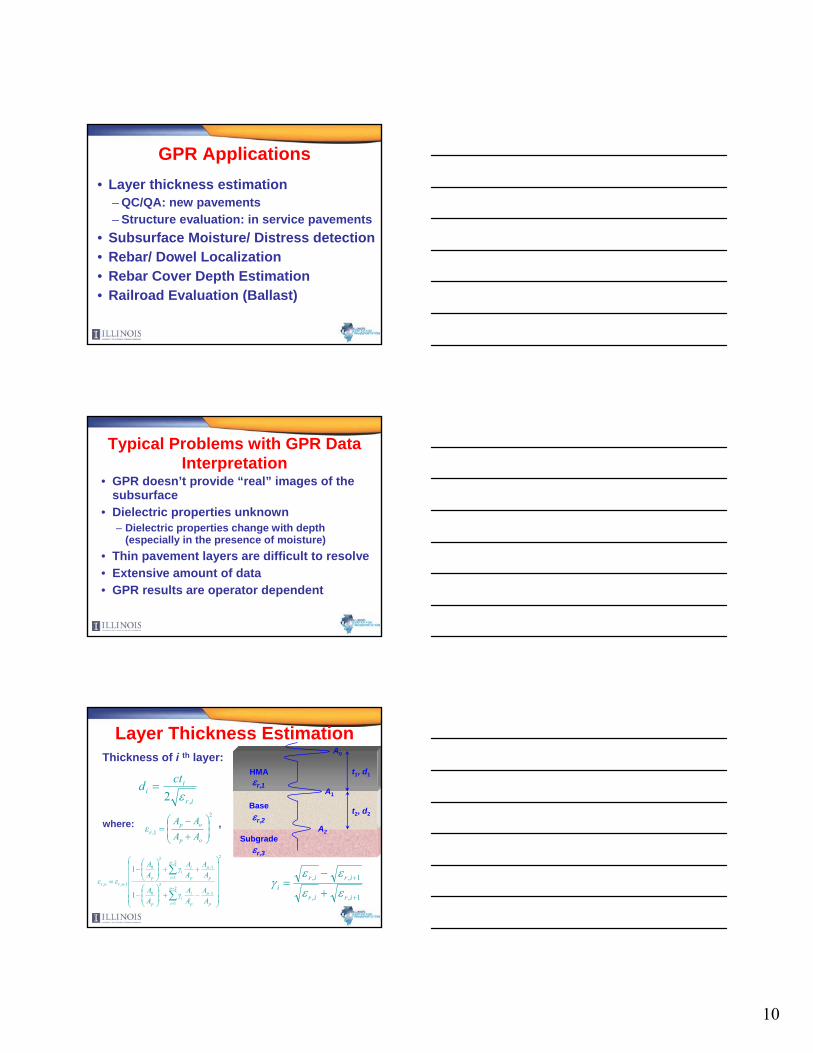
GPR Applications• Layer thickness estimation

– QC/QA: new pavements– Structure evaluation: in service pavements

• Subsurface Moisture/ Distress detection• Rebar/ Dowel Localization• Rebar Cover Depth Estimation• Railroad Evaluation (Ballast)

Typical Problems with GPR Data Interpretation

• GPR doesn’t provide “real” images of the subsurface

• Dielectric properties unknown– Dielectric properties change with depth

(especially in the presence of moisture)• Thin pavement layers are difficult to resolve• Extensive amount of data• GPR results are operator dependent

Layer Thickness Estimation

2

12

1

2

0

12

1

2

0

1,,

1

1

⎟⎟⎟⎟⎟⎟

⎠

⎞

⎜⎜⎜⎜⎜⎜

⎝

⎛

−+⎟⎟⎠

⎞⎜⎜⎝

⎛−

++⎟⎟⎠

⎞⎜⎜⎝

⎛−

=−

−

=

−−

=

∑

∑

p

nn

i p

ii

p

p

nn

i p

ii

pn-rnr

AA

AAγ

AA

AA

AAγ

AA

εε

Thickness of i th layer:HMA

Base

Subgrade

t1, d1

t2, d2

A0

A1

A2

εr,1

εr,2

εr,3

1,,

1,,

+

+

+

−=

irir

iriri εε

εεγ

where: ,2

1, ⎟⎟⎠

⎞⎜⎜⎝

⎛

+

−=

op

opr AA

AAε

ir

ii

ctd,2 ε

=

11

BM-25.0

GPR: EMBEDDED COPPER PLATES

1

2

34

Subgrade/21B

21B/21A

OGDL/21A

BM-25.0/OGDL

Fi ρ

1+ρ

(1+ρ)*T −(1+ρ)*T

−(1+ρ)*T2

−(1−ρ2)*T2

ρ∗(1+ρ)*T2

ρ∗(1+ρ)*T3

−ρ∗(1+ρ)*T3

−ρ∗(1+ρ)*T4

−ρ(1−ρ2)*T4

ρ2∗(1+ρ)*T4

ρ2∗(1+ρ)*T5

−ρ2∗(1+ρ)*T5

−ρ2∗(1+ρ)*T6

−ρ2∗(1−ρ2)*T6

d

Copper Plate

Multiple Reflection Model

WS Dielectric Constant

*r

*r

1

-1

ε+

ε=ρ

ddρ+1ρ−ω

−εω

−==

1c

j*rc

jeeT

∑=

2222

+222 ρΤρ−Τ − ρ=

ρΤ−ρΤ−

ρ−Τ − ρ===Γn

1i

i1n

i

r

i

r )()1(1

)(1)1(FF

)FT(Y)FT(Y

0FF

1)(1)1((f

i

r1n

=−ρΤ−

ρΤ−ρ−Τ − ρ=ρ)

2

+222

Input Reflection Coefficient

with: and

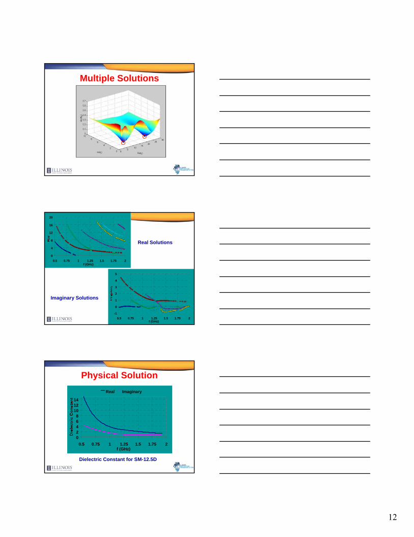
To find εr, Solve:

12

Multiple Solutions

0

4

8

12

16

20

0.5 0.75 1 1.25 1.5 1.75 2f (GHz)

-1

0

1

2

3

4

5

0.5 0.75 1 1.25 1.5 1.75 2f (GHz)

Real Solutions

Imaginary Solutions

02468

101214

0.5 0.75 1 1.25 1.5 1.75 2f (GHz)

Real Imaginary

Dielectric Constant for SM-12.5D

Physical Solution

13

Thickness Estimation Using CMP Technique (more accurate)

Common midpoint (CMP) technique (or common-depth point, CDP) is used as follows:

T/RT R

x

t1

t2

P

HMAεr1

h

ν : EM velocity in the layer ( )

2

21

22

2

xttc

r−

=εhvt 21 =

22

2 22 ⎟

⎠⎞

⎜⎝⎛+=

xhvt

21

22rε tt

xcv−

==

⇒

Thickness Estimation Using Modified CMP Technique

h1

T/R

x0

t1

t2

P

HMAεr1

h0

airεr0=1

x1

T R

θi

θt

21

22

1

ttxv−

=

trir θsinεθsinε 10 =

01i0 θtan2 xxh =+

1

1

1

1t 2θtan

vtx

hx

==

Snell’s law of refraction:

Using the figure:

(1)

(2)

(3)

(4)

Thickness Estimation Using Modified CMP Technique Algorithm:

1. Measure the reflection times t1 and t2

2. Calculate the transmission angle θt using:3. Find the angle θi by solving numerically

4. Solve for εr1 using:

5. Compute HMA thickness using t1 and εr1

1

21

22

tθtant

tt −=

021

22

i

ti0 θsin

θsinθtan2 xttch =−+

2

t

i1 θsin

θsin⎟⎟⎠

⎞⎜⎜⎝

⎛=rε

111 2 rcth ε=

Modified CMP Setup

14

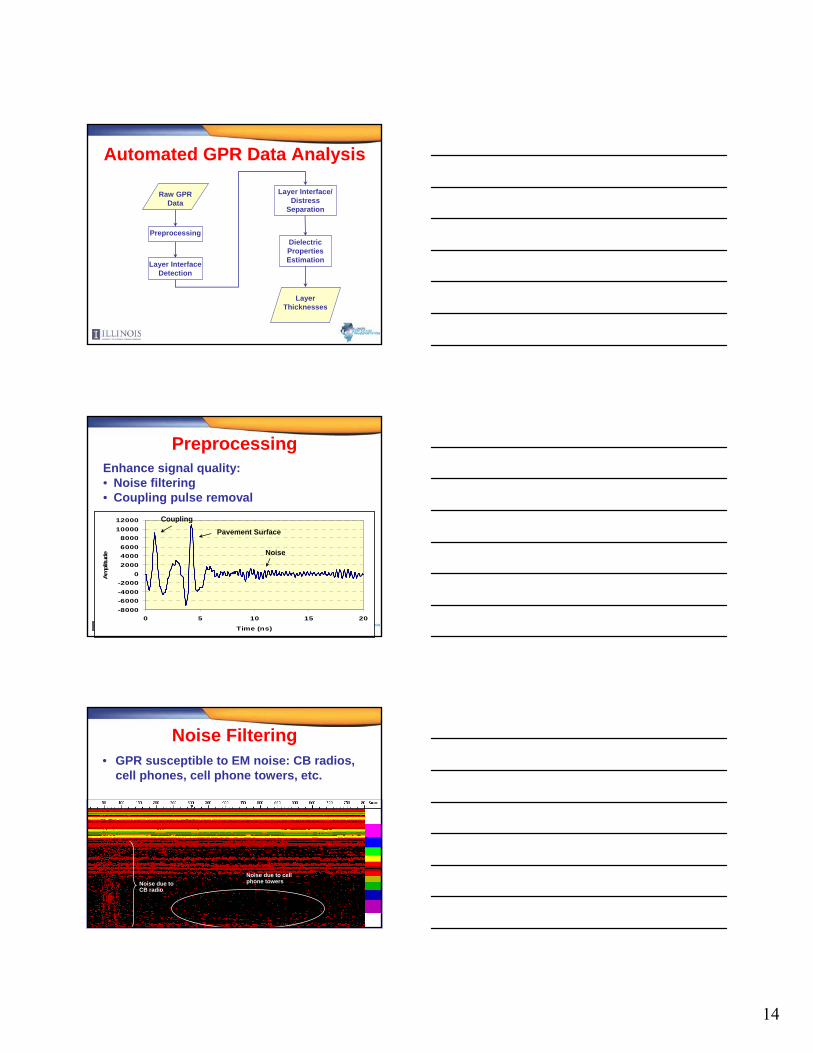
Automated GPR Data Analysis

Raw GPR Data

Layer Interface Detection

Dielectric Properties Estimation

Layer Thicknesses

Preprocessing

Layer Interface/ Distress

Separation

PreprocessingEnhance signal quality:• Noise filtering• Coupling pulse removal

-8000-6000-4000-2000

02000400060008000

1000012000

0 5 10 15 20

Time (ns)

Am

plitu

de

Pavement Surface

Noise

Coupling

Noise Filtering• GPR susceptible to EM noise: CB radios,

cell phones, cell phone towers, etc.

Noise due to CB radio

Noise due to cell phone towers

15

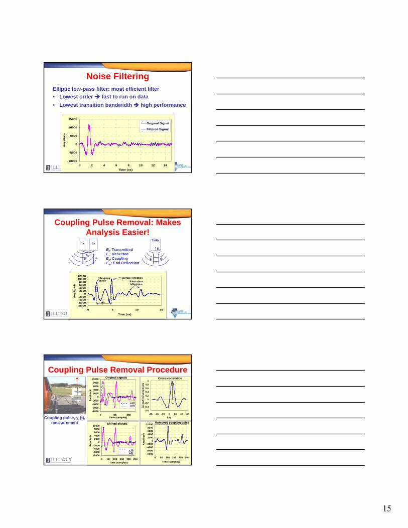
Noise FilteringElliptic low-pass filter: most efficient filter• Lowest order fast to run on data• Lowest transition bandwidth high performance

-10000

-5000

0

5000

10000

15000

0 2 4 6 8 10 12 14Time (ns)

Am

plitu

de

Original Signal

Filtered Signal

Coupling Pulse Removal: Makes Analysis Easier!

Tx Rx

Et

EcEr

Tx/Rx

Et Er

EerEt: TransmittedEr: Reflected Ec: CouplingEer: End Reflection

-8000-6000-4000-2000

02000400060008000

1000012000

0 5 10 15Time (ns)

Am

plitu

tde

Coupling pulse

Surface reflectionSubsurface reflections

Air

Coupling Pulse Removal Procedure

-0.6-0.4-0.2

00.20.40.60.8

1

-60 -40 -20 0 20 40 60Lag

Nor

mal

ized

Am

plitu

de

lm

Cross-correlation

-8000-6000-4000-2000

02000400060008000

10000

0 100 200Time (samples)

Am

plitu

de

yc(t)yr(t)

Original signals

-8000-6000-4000-2000

02000400060008000

10000

0 50 100 150 200 250Time (samples)

Am

plitu

de

yc(t)yr(t)

Shifted signals

-8000-6000-4000-2000

02000400060008000

10000

0 50 100 150 200 250Time (samples)

Am

plitu

de

Removed coupling pulseCoupling pulse, yc(t),

measurement

16

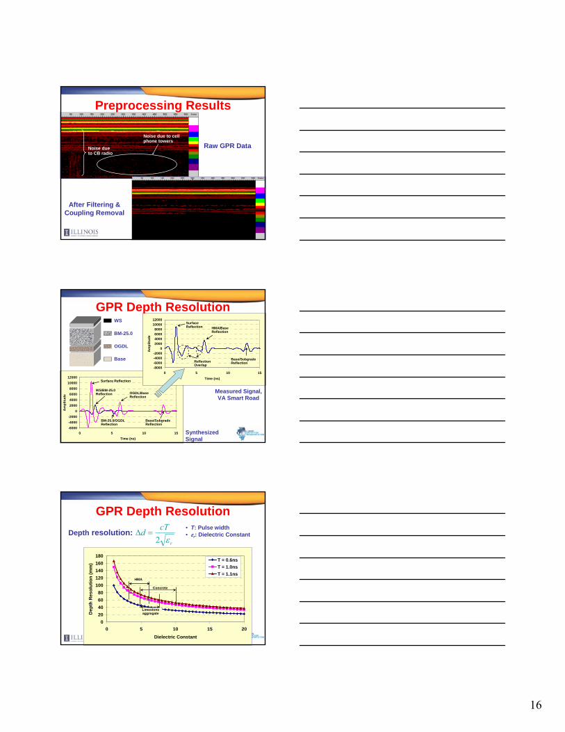
Preprocessing Results

Noise due to CB radio

Noise due to cell phone towers

Raw GPR Data

After Filtering & Coupling Removal

GPR Depth Resolution

-6000-4000-2000

02000400060008000

1000012000

0 5 10 15Time (ns)

Am

plitu

de

-8000-6000-4000-2000

02000400060008000

1000012000

0 5 10 15Time (ns)

Am

plitu

de

Measured Signal, VA Smart Road

Synthesized Signal

Surface Reflection

OGDL/Base Reflection

WS/BM-25.0 Reflection

BM-25.0/OGDL Reflection

Base/Subgrade Reflection

Reflection Overlap

Surface Reflection HMA/Base

Reflection

Base/Subgrade Reflection

Base

OGDL

WS

BM-25.0

GPR Depth Resolution

r

cTdε2

=ΔDepth resolution:• T: Pulse width• εr: Dielectric Constant

020406080

100120140160180

0 5 10 15 20Dielectric Constant

Dep

th R

esol

utio

n (m

m)

T = 0.6nsT = 1.0nsT = 1.1ns

HMA

Limestone aggregate

Concrete

17

GPR Detection Limitations

Copper Plate Reflections at the (1) 21B/Subgrade, (2) 21A/21B, (3) OGDL/21A, (4) BM-25.0/OGDL, and (5) WS/BM-

25.0 Interfaces; Section A

1

2

34

5

Depth

Pavement Surface

OGDL/21A Interface

Spurious interface reflection

21A

OGDL

WS

BM-25.0

21B

Subgrade

Depth Resolution Enhancement

• Inverse filtering• Predictive deconvolution• Pulse spiking• Pulse shaping• Homomorphic deconvolution

Wiener Filter

Inverse Filtering• Implemented as a Wiener filter• Desired output: impulse at time t=0 ⇒ δ(t)• Incident signal assumed unknown• Filter designed according to:

⎥⎥⎥⎥⎥⎥

⎦

⎤

⎢⎢⎢⎢⎢⎢

⎣

⎡

=

⎥⎥⎥⎥⎥⎥

⎦

⎤

⎢⎢⎢⎢⎢⎢

⎣

⎡

⎥⎥⎥⎥⎥⎥

⎦

⎤

⎢⎢⎢⎢⎢⎢

⎣

⎡

−

−−−

− 0

001

)0()1(

)3()0()2()2()1()0()1()1()2()1()0(

1

2

1

0

MM

LLL

MOM

L

L

Nyyyy

yyyyyy

yyyyyyyy

yyyyyyyy

a

aaa

rNr

NrrrNrrrrNrrrr

18

Predictive Deconvolution• Implemented as a Wiener filter• Desired output: reflected signal

advanced by α samples ⇒ y(t+ α)• Incident signal assumed unknown• Filter designed according to:

⎥⎥⎥⎥⎥⎥

⎦

⎤

⎢⎢⎢⎢⎢⎢

⎣

⎡

−+

++

=

⎥⎥⎥⎥⎥⎥

⎦

⎤

⎢⎢⎢⎢⎢⎢

⎣

⎡

⎥⎥⎥⎥⎥⎥

⎦

⎤

⎢⎢⎢⎢⎢⎢

⎣

⎡

−

−−−

− )1(

)2()1(

)(

)0()1(

)3()0()2()2()1()0()1()1()2()1()0(

1

2

1

0

Nr

rr

r

a

aaa

rNr

NrrrNrrrrNrrrr

yy

yy

yy

yy

Nyyyy

yyyyyy

yyyyyyyy

yyyyyyyy

α

αα

α

MM

LLL

MOM

L

L

Pulse Spiking• Implemented as a Wiener filter• Desired output: an impulse (or spike) at

a lag l• Incident signal should be known• Filter designed according to:

⎥⎥⎥⎥⎥⎥⎥⎥⎥

⎦

⎤

⎢⎢⎢⎢⎢⎢⎢⎢⎢

⎣

⎡−

=

⎥⎥⎥⎥⎥⎥

⎦

⎤

⎢⎢⎢⎢⎢⎢

⎣

⎡

⎥⎥⎥⎥⎥⎥

⎦

⎤

⎢⎢⎢⎢⎢⎢

⎣

⎡

−

−−−

−

0

0)0(

)1()(

)0()1(

)3()0()2()2()1()0()1()1()2()1()0(

1

2

1

0

M

M

M

LLL

MOM

L

L

x

lxlx

a

aaa

rNr

NrrrNrrrrNrrrr

Nxxxx

xxxxxx

xxxxxxxx

xxxxxxxx

Pulse Shaping• Implemented as a Wiener filter• Desired output: a pulse with a fixed

shape s(t) at a given lag l• Incident signal should be known• Filter designed according to:

⎥⎥⎥⎥⎥⎥

⎦

⎤

⎢⎢⎢⎢⎢⎢

⎣

⎡

−+

++

=

⎥⎥⎥⎥⎥⎥

⎦

⎤

⎢⎢⎢⎢⎢⎢

⎣

⎡

⎥⎥⎥⎥⎥⎥

⎦

⎤

⎢⎢⎢⎢⎢⎢

⎣

⎡

−

−−−

− )1(

)2()1(

)(

)0()1(

)3()0()2()2()1()0()1()1()2()1()0(

1

2

1

0

Nlr

lrlr

lr

a

aaa

rNr

NrrrNrrrrNrrrr

sx

sx

sx

sx

Nxxxx

xxxxxx

xxxxxxxx

xxxxxxxx

MM

LLL

MOM

L

L

19

Homomorphic Deconvolution• Power cepstrum of signal y(t):

• For GPR reflected signals:

• Term inside brackets periodic function of time delays ⇒ Power cepstrum composed of pulses corresponding to time-delays

{ }[ ]{ }22)(log)( tyFFqC y =

[ ] [ ]2

1

1 10

20 )2cos(2log)(log)(

⎭⎬⎫

⎩⎨⎧

∑++Φ≈ ∑−

= =

N

n

n

ii

nxy tf

AA

AfFqC π

Typical Results

-0.15

-0.1

-0.05

0

0.05

0.1

0.15

0 5 10 15 20Time (ns)

Am

plitu

de

Surface

OGDL/BaseWS/BM-25.0

BM-25.0/OGDL

Base/Subgrade

-6000

-4000

-2000

0

2000

4000

6000

8000

10000

0 5 10 15 20Time (ns)

Am

plitu

de

Surface

OGDL/BaseWS/BM-25.0

BM-25.0/OGDL Base/Subgrade0

500

1000

1500

2000

2500

0 2 4 6 8 10 12 14 16 18 20Time (ns)

Am

plitu

de

Surface

OGDL/BaseWS/BM-25.0

Base/Subgrade

-8000-6000-4000-2000

02000400060008000

1000012000

0 5 10 15Time (ns)

Am

plitu

de

HomomorphicPulse Spiking

Inverse FilteringOriginal

Typical Results: Inverse Filtering

HMA Layers

Base LayerMultiple Reflections from Copper Plates

WSBM-25.0

OGDL

Raw Data,VA. Smart Road, Section A

Processed Data

20

Resolving Thin Layers (Deconvolution)

21A

OGDL

WS

BM-25.0

21B1

2

34

5

Depth

Pavement Surface

OGDL/21A Interface

Spurious Interface Reflection

1

2

34

5

Depth

Pavement Surface

OGDL/21A Interface

WS

BM-25.0

OGDL

Base

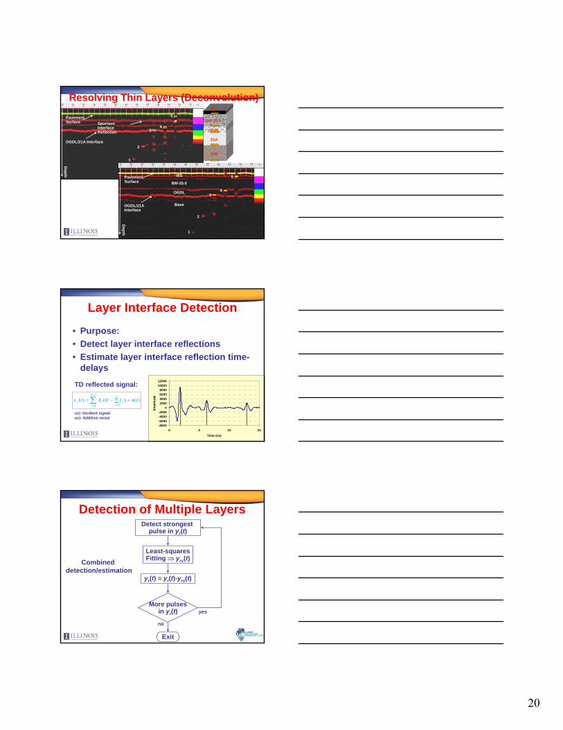
Layer Interface Detection

• Purpose:• Detect layer interface reflections• Estimate layer interface reflection time-

delays

-8000-6000-4000-2000

02000400060008000

1000012000

0 5 10 15Time (ns)

Am

plitu

de)()()(1

0 0tnttxAty

N

i

i

jjir +∑−= ∑

−

= =

TD reflected signal:

x(t): Incident signaln(t): Additive noise

Detection of Multiple Layers

Combineddetection/estimation

Detect strongest pulse in yr(t)

Least-squaresFitting ⇒ yrs(t)

yr(t) = yr(t)-yrs(t)

More pulsesin yr(t) yes

no

Exit

21

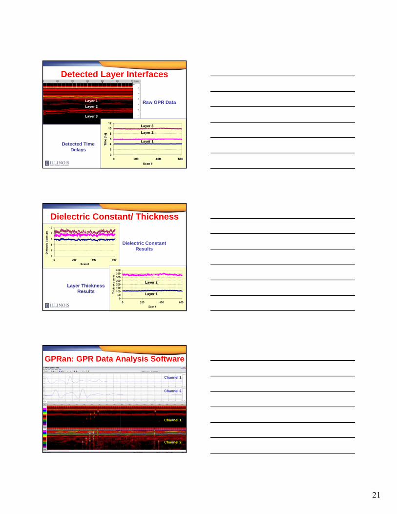
Detected Layer Interfaces

Raw GPR Data

Detected Time Delays

Layer 1

Layer 2

Layer 3

Layer 1Layer 2

Layer 3

Dielectric Constant Results

Layer Thickness Results

Dielectric Constant/ Thickness

Layer 1

Layer 2

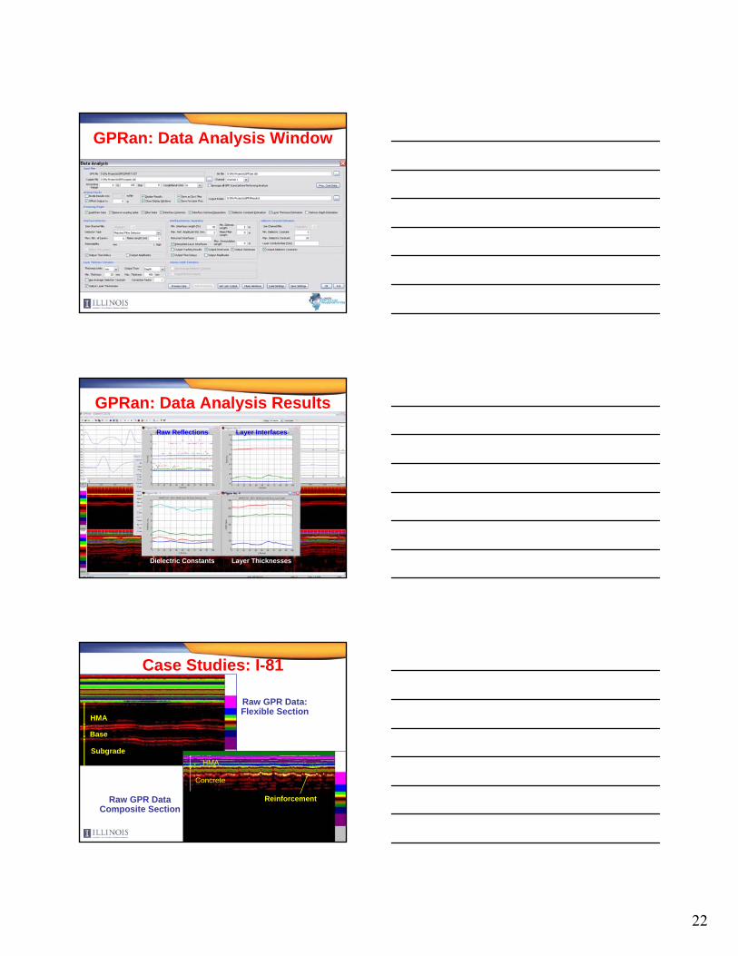
GPRan: GPR Data Analysis Software

Channel 1

Channel 2

Channel 1

Channel 2

22

GPRan: Data Analysis Window

GPRan: Data Analysis ResultsRaw Reflections Layer Interfaces

Dielectric Constants Layer Thicknesses

HMA

Base

SubgradeHMA

Reinforcement

Concrete

Raw GPR Data: Flexible Section

Raw GPR Data Composite Section

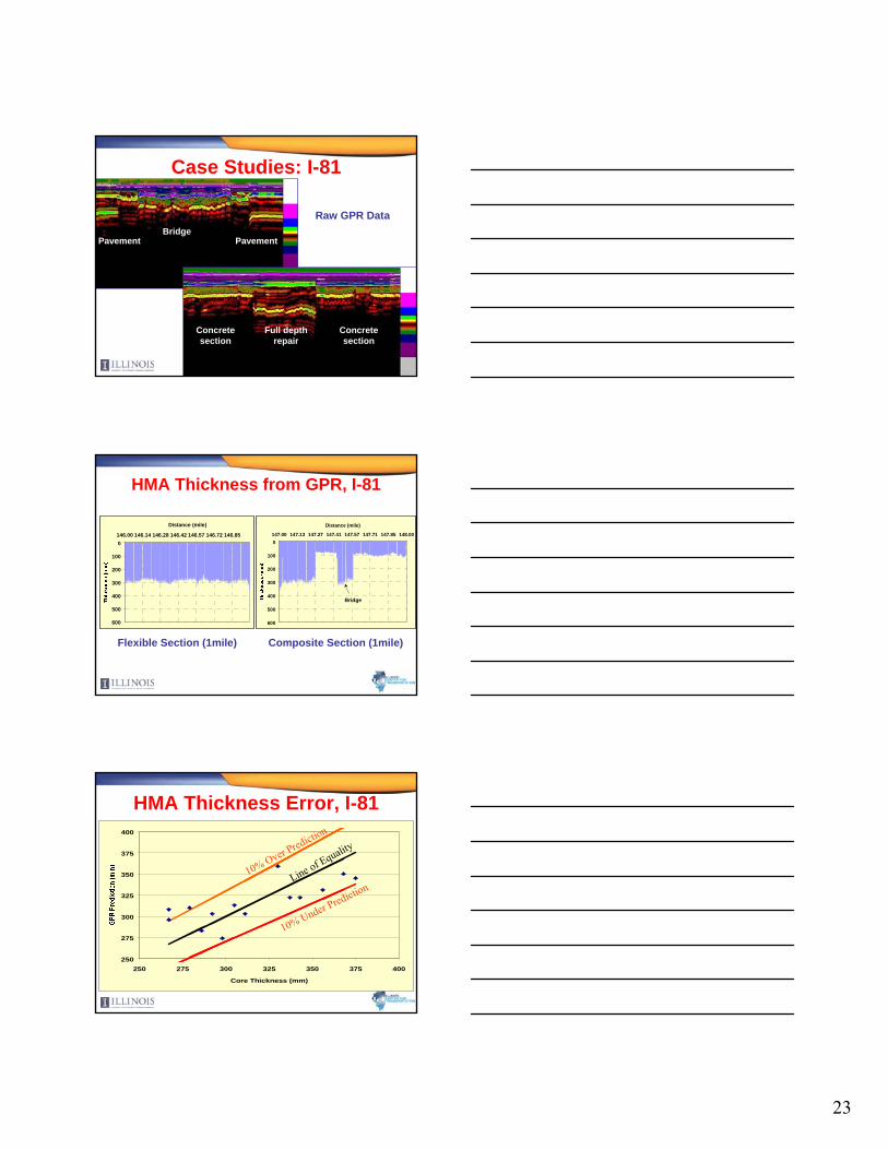
Case Studies: I-81

23

BridgePavementPavement

Concrete section

Concrete section

Full depth repair

Case Studies: I-81

Raw GPR Data

0

100

200

300

400

500

600

146.00 146.14 146.28 146.42 146.57 146.72 146.85

Distance (mile)

0

100

200

300

400

500

600

147.00 147.13 147.27 147.41 147.57 147.71 147.85 148.00

Distance (mile)

Bridge

Flexible Section (1mile) Composite Section (1mile)

HMA Thickness from GPR, I-81

HMA Thickness Error, I-81

250

275

300

325

350

375

400

250 275 300 325 350 375 400

Core Thickness (mm)

Line of Equality

10% Over Prediction

10% Under Prediction

24

QA/QC New Pavement (VA Rt. 288)

21-B aggregate base

IM-19.0 (1) w/ PG 64-22

BM-25.0 w/ PG 64-22

SM-12.5 w/ PG 76-22

IM-19.0 (2) w/ PG 76-22

150mm (6in)

300mm (12in)

100mm (4in)

75mm (3in)

65mm (2.6in)

50mm (2in)

Lime stabilized subgrade

Pavement design:

• GPR surveys were performed on each layer after its construction

• Three surveys were performed per lane and per layer; in total, 36 surveys were performed

• DMI set at 10 scans/m• For HMA layers, static

measurements were taken near core locations

9.8m 9m 8.2m 6.2m 5.4m 4.6m 2.6m 1.8m 1m

HMA Base CoresHMA Intermediate 1 CoresHMA Intermediate 2 Cores

1

2

3

4

5

6

7

8

9

10

11

12

13

14

15

16

S1S2

QA/QC1

QA/QC2

QA/QC3

QA/QC4

QA/QC5

QA/QC6

Station 189 + 80

Station 186 + 10

Survey Direction

Offset

Right Lane Center Lane Left Lane

GPR Data Collection (Rt. 288)

Typical GPR Response (Rt. 288)

-8000-6000-4000-2000

02000400060008000

1000012000

0 1 2 3 4 5 6 7 8 9 10 11 12

Time (ns)

Am

plitu

de

21B Coupling Surface

Air

GPR Scan over 21-B Layer

GPR Scan over HMA Intermediate 2

-8000-6000-4000-2000

02000400060008000

1000012000

0 1 2 3 4 5 6 7 8 9 10 11 12

Time (ns)

Am

plitu

de 21BHMA

25

21-B Thickness (Rt 288)

0

50

100

150

200

250

300

350

0 20 40 60 80 100 120 140 160 180

Distance (m)

Thic

knes

s (m

m)

Offset 6.2mOffset 5.4mOffset 4.6mDesign

0

50

100

150

200

250

300

350

184 204 224 244 264 284 304 324 344 364

Distance (m)

Thic

knes

s (m

m)

Offset 6.2mOffset 5.4mOffset 4.6mDesign

Center Lane, 0-184 m

Center Lane, 184-370 m

Offset values are with respect to left edge of left lane

HMA Intermediate-2 Thickness (Rt 288)

Center Lane, 0-184 m

Center Lane, 184-370 m

0

50

100

150

200

250

300

350

0 20 40 60 80 100 120 140 160 180

Distance (m)

Thic

knes

s (m

m)

Offset 6.2mOffset 5.4mOffset 4.6mDesign

0

50

100

150

200

250

300

350

184 204 224 244 264 284 304 324 344 364

Distance (m)

Thic

knes

s (m

m)

Offset 6.2mOffset 5.4mOffset 4.6mDesign

Offset values are with respect to left edge of left lane

Overall Thickness (Rt 288)

050

100150200250300350400450500

40 42.5 45 47.5 50 52.5 55 57.5 60Distance (m)

Dep

th (m

m)

HMA Base

HMA Design Base Design

26

020406080

100120140160180200220

9.8 9 8.2 6.2 5.4 4.6 2.6 1.8 1Offset (m)

Offset values are with respect to left edge of left lane

Average Thickness, 21-B Layer

Average Thickness, HMA Base Layer

Right

02 04 06 08 01 00

1 2 01 4 01 6 01 8 02 002 2 0

2 4 02 6 02 8 03 003 2 0

9 . 8 9 8 .2 6 .2 5 .4 4 .6 2 .6 1 . 8 1O ffse t (m)

Thick. 0-184mThick. 184-370mStd. Dev. 0-184mStd. Dev. 184-370m

Center Left

0

20

40

60

80

100

120

140

160

9.8 9 8.2 6.2 5.4 4.6 2.6 1.8 1Offset (m)

Right Center Left

GPR Accuracy (Rt 288)

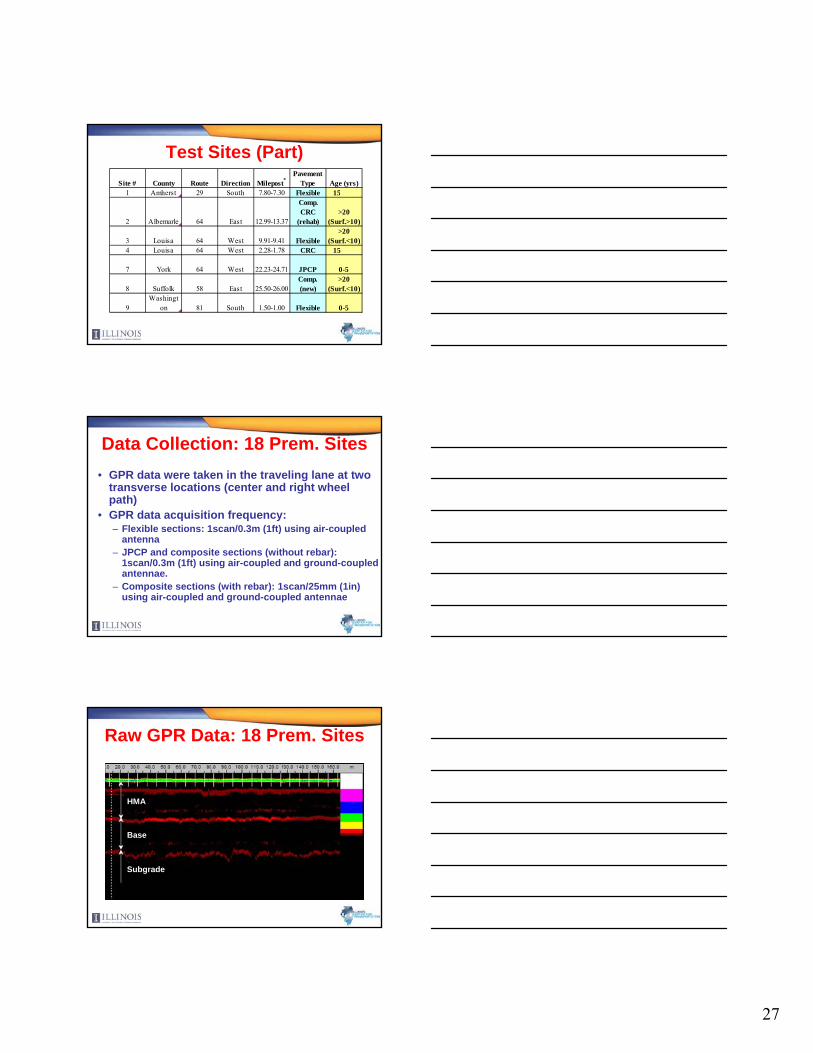
Case Study: 18 Premium Pavement Sites

• Sites located mainly on highways • Different types of pavements were tested:

– Full-depth flexible pavement– Rigid (jointed plain concrete pavement

(JPCP)– Continuously reinforced concrete

(CRCP)– Composite pavement

• Each section was 0.8 km (0.5 mile) long

27

Test Sites (Part)Site # County Route Direction Milepost*

Pavement Type Age (yrs)

1 Amherst 29 South 7.80-7.30 Flexible 15-Oct

2 Albemarle 64 East 12.99-13.37

Comp. CRC

(rehab)>20

(Surf.>10)

3 Louisa 64 West 9.91-9.41 Flexible>20

(Surf.<10)4 Louisa 64 West 2.28-1.78 CRC 15-Oct

7 York 64 West 22.23-24.71 JPCP 0-5

8 Suffolk 58 East 25.50-26.00Comp. (new)

>20 (Surf.<10)

9Washingt

on 81 South 1.50-1.00 Flexible 0-5

Data Collection: 18 Prem. Sites• GPR data were taken in the traveling lane at two

transverse locations (center and right wheel path)

• GPR data acquisition frequency:– Flexible sections: 1scan/0.3m (1ft) using air-coupled

antenna– JPCP and composite sections (without rebar):

1scan/0.3m (1ft) using air-coupled and ground-coupled antennae.

– Composite sections (with rebar): 1scan/25mm (1in) using air-coupled and ground-coupled antennae

Raw GPR Data: 18 Prem. Sites

HMA

Base

Subgrade

28

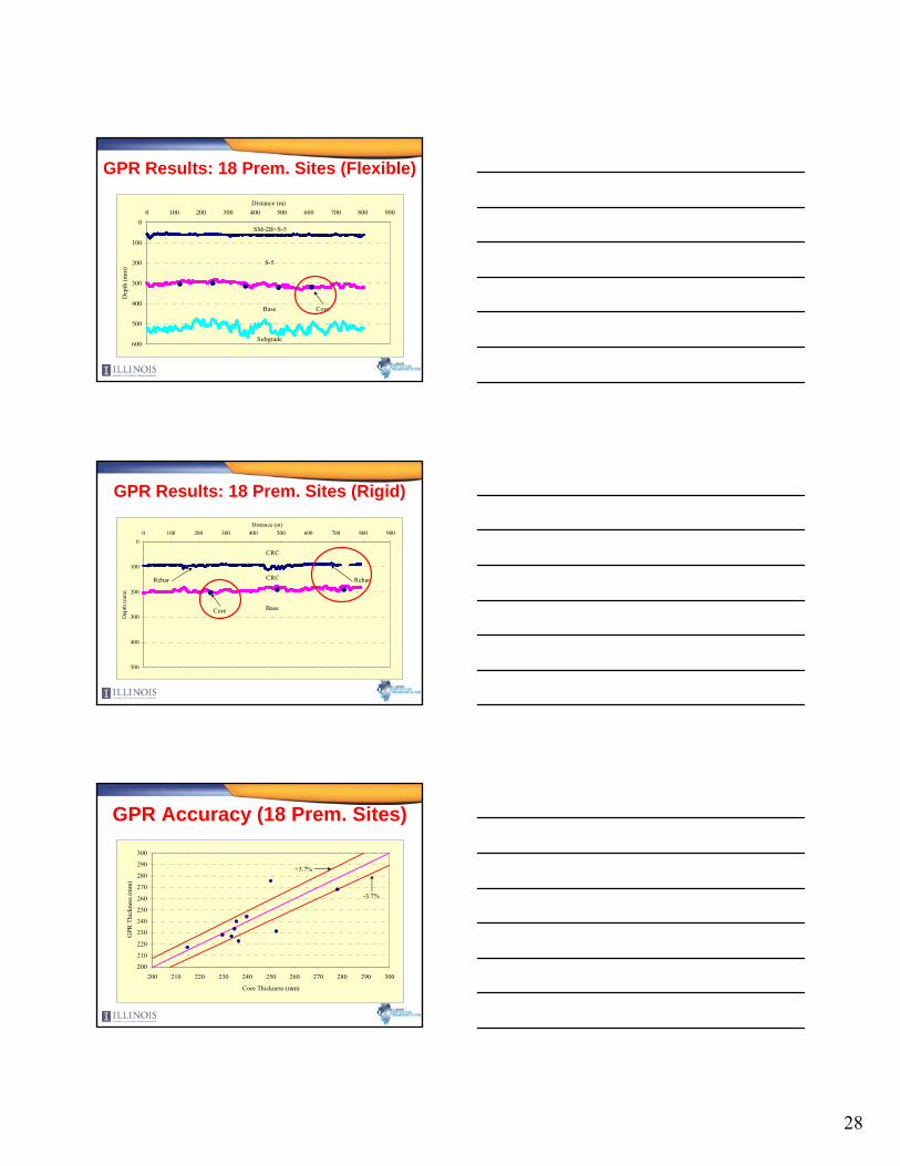
GPR Results: 18 Prem. Sites (Flexible)

0

100

200

300

400

500

600

0 100 200 300 400 500 600 700 800 900Distance (m)

Dep

th (m

m)

SM-2B+S-5

Base

S-5

Subgrade

Core

GPR Results: 18 Prem. Sites (Rigid)

0

100

200

300

400

500

0 100 200 300 400 500 600 700 800 900Distance (m)

Dep

th (m

m)

CRC

Base

CRC RebarRebar

Core

GPR Accuracy (18 Prem. Sites)

200

210

220

230

240

250

260

270

280

290

300

200 210 220 230 240 250 260 270 280 290 300

Core Thickness (mm)

GPR

Thi

ckne

ss (m

m)

+3.7%

-3.7%

29

Average Error per Site (18 Prem. Sites)

3.7

6.0

4.7

1.8

3.2

8.2

2.3

3.2

5.3

3.1

4.14.8

5.6 5.4

8.4

4.64.0

0

1

2

3

4

5

6

7

8

9

1 2 3 4 5 6 7 8 9 10 11 12 13 15 16 17 18

Site #

GPR

Abs

olut

e Er

ror (

%)

Average Error per Age (18 Prem. Sites)

4.4 4.6 4.9

5.8

0

1

2

3

4

5

6

7

0-5 10 -- 15 >20 (Surf.<10) >20 (Surf.>10)

Pavement Age (years)

Ave

rage

GPR

Thi

ckne

ss E

rror

(%)

Average Error per Type (18 Prem. Sites)4.4

2.3

00.5

11.5

22.5

33.5

44.5

5

Flexible JPCP

Pavement Type

GPR

Thi

ckne

ss E

rror

(%)

3.0

4.2

00.5

11.5

22.5

33.5

44.5

CRC Flexible

Pavement Type

Ave

rage

GPR

Thi

ckne

ss E

rror

(%)

Pavement Age: 0-5 yrs

Pavement Age: 10-15 yrs

30

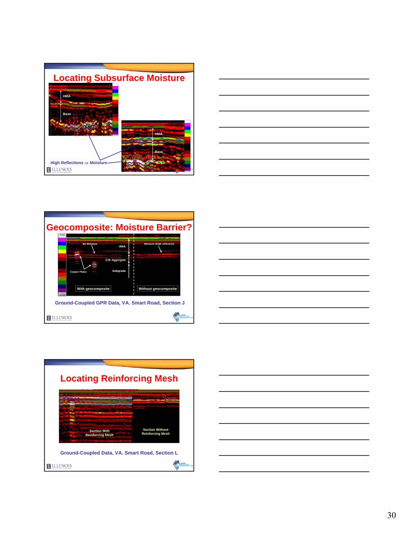
High Reflections ⇒ Moisture

Locating Subsurface Moisture

HMA

Base

HMA

Base

Ground-Coupled GPR Data, VA. Smart Road, Section J

Without geocompositeWith geocomposite

HMA

21B Aggregate

Copper Plates Subgrade

Geocomposite: Moisture Barrier?Moisture (high reflection)No Moisture

Locating Reinforcing Mesh

Section With Reinforcing Mesh

Section Without Reinforcing Mesh

Ground-Coupled Data, VA. Smart Road, Section L

31

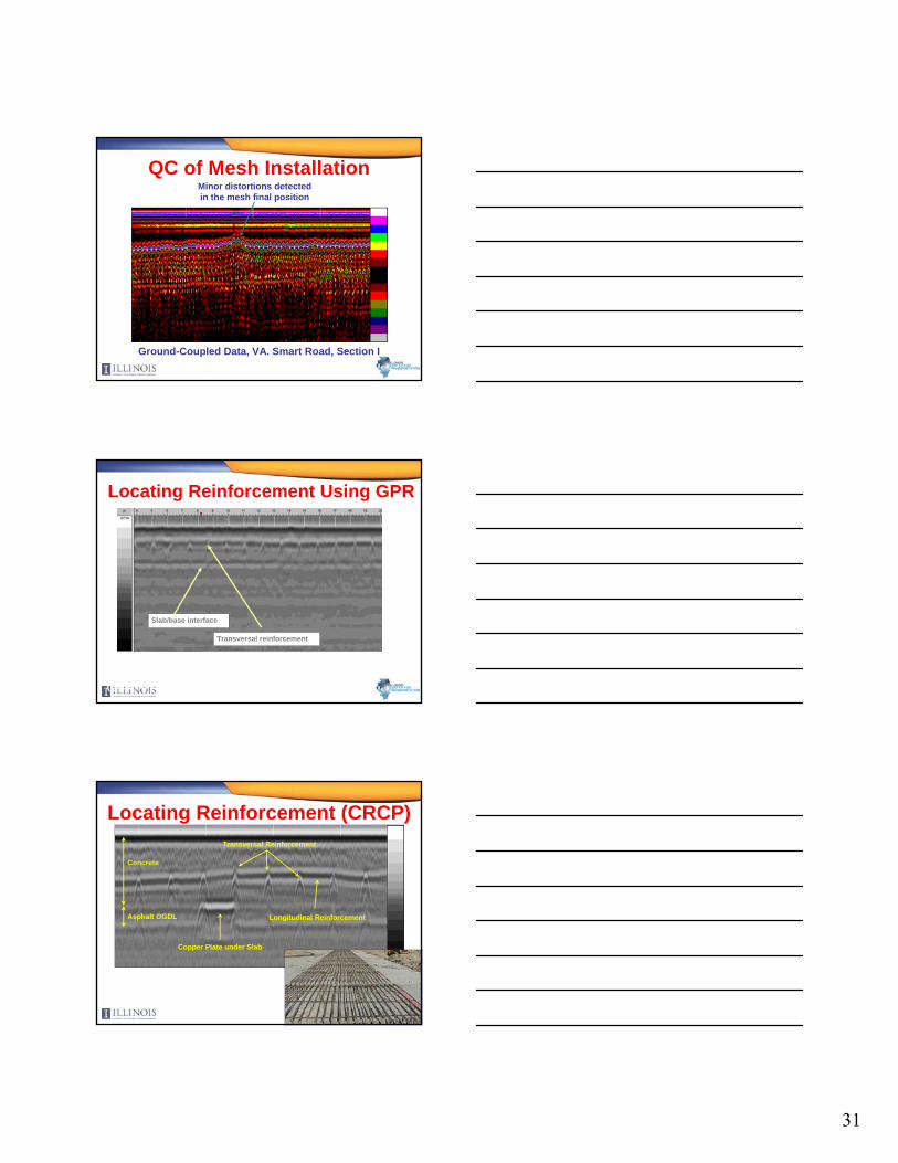
Minor distortions detected in the mesh final position

QC of Mesh Installation

Ground-Coupled Data, VA. Smart Road, Section I

Slab/base interface

Transversal reinforcement

CRCP(ground-coupled)

Locating Reinforcement Using GPR

Locating Reinforcement (CRCP)

Copper Plate under Slab

Transversal Reinforcement

Concrete

Asphalt OGDL Longitudinal Reinforcement

32

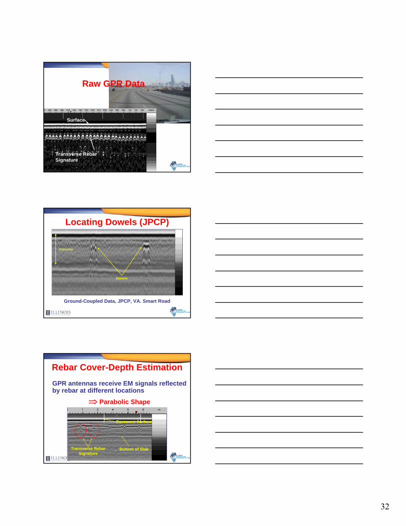
Raw GPR Data

Surface

Transverse Rebar Signature

Ground-Coupled Data, JPCP, VA. Smart Road

Locating Dowels (JPCP)

Dowels

Concrete

Rebar Cover-Depth EstimationGPR antennas receive EM signals reflected by rebar at different locations

⇒ Parabolic Shape

Pavement Surface

Transverse RebarSignature

Bottom of Slab

33

GPR Data Collection

Concrete

Concrete

Rebar

Rebar Cover-Depth Estimation

GPR GPR GPR

Survey direction

Concrete slab εr

Transverse rebar

x

t0, d0 t, d

x0

Survey configuration on CRCP

Rebar Cover-Depth Estimation

From the previous configuration we have:

2

202

0202

22 484

vxtx

vxx

vt ++−=

r

cvε

=with:

34

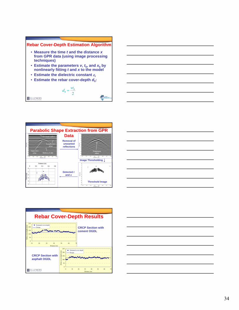
Rebar Cover-Depth Estimation Algorithm• Measure the time t and the distance x

from GPR data (using image processing techniques)

• Estimate the parameters v, t0, and x0 by nonlinearly fitting t and x to the model

• Estimate the dielectric constant εr• Estimate the rebar cover-depth d0:

20

0vtd =

Parabolic Shape Extraction from GPR Data

Transverse rebar

Removal of unwanted reflections

Image Thresholding

Detected tand x

Threshold Image

Rebar Cover-Depth Results

0

50

100

150

200

250

10 20 30 40 50 60 70

Distance (m)

Reb

ar c

over

-dep

th (m

m) Estimated cover-depth

Design CRCP Section with cement OGDL

0

50

100

150

200

250

0 10 20 30 40 50 60 70Distance (m)

Reb

ar c

over

-dep

th (m

m) Estimated cover-depth

Design

CRCP Section with asphalt OGDL

35

Rebar Cover-Depth Accuracy

Comparison of GPR estimated cover-depth to CRCP cores from the VA Smart Road

Core 1 145 141 2.8Core 2 121 118 2.5

2.6Average error (%)

Core cover-depth (mm)

GPR cover-depth (mm)

Error (%)

Supe

rstr

uctu

reSu

bstr

uctu

re

Rail

Bal

last

Ballast

Subballast

Fastening System

Vertical

Longitudinal

Crib

Tie

Ballast

Placed Soil (Fill)

Natural Ground (Formation)

Subgrade(Platform)

Railroad Structure

Clean and Fouled Ballast

• Clean ballast : made of uniformly graded aggregates ⇒ large air voids.

• Fouled ballast : fouled by fine-grained material that the fills air-voids.

Ballast fouling greatly influences its functions:

36

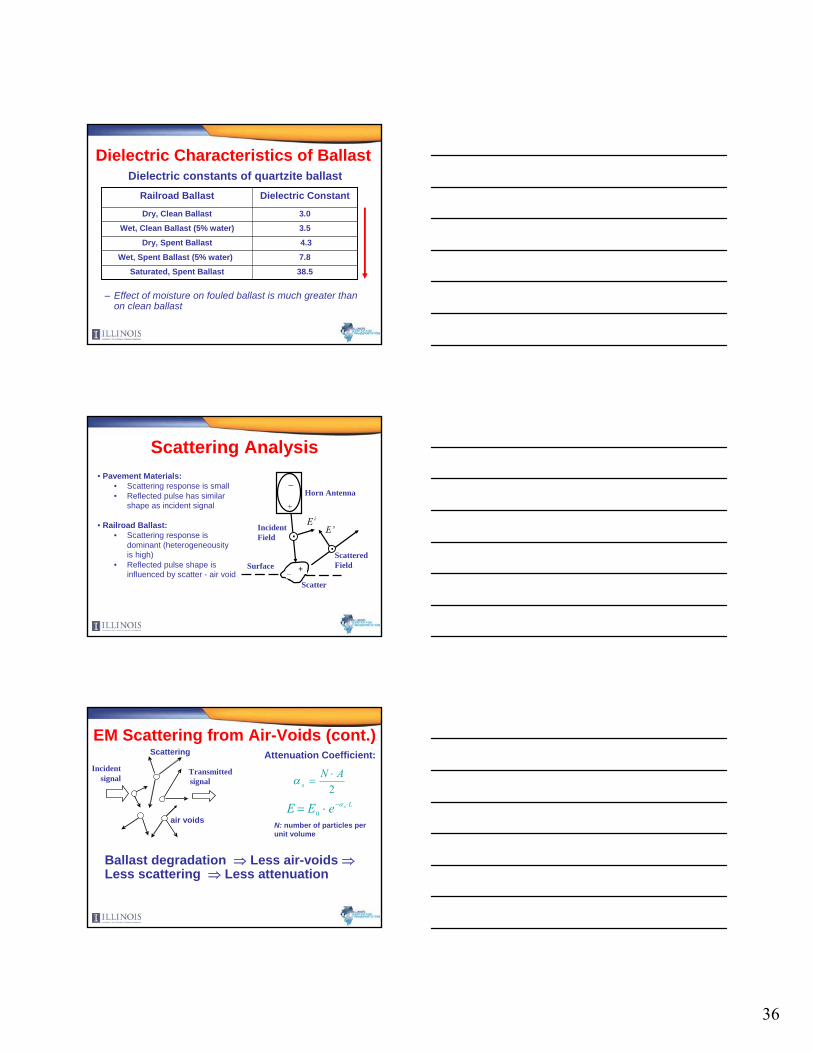
Dielectric Characteristics of Ballast

38.5Saturated, Spent Ballast

7.8Wet, Spent Ballast (5% water)

4.3Dry, Spent Ballast

3.5Wet, Clean Ballast (5% water)

3.0Dry, Clean Ballast

Dielectric ConstantRailroad Ballast

Dielectric constants of quartzite ballast

– Effect of moisture on fouled ballast is much greater than on clean ballast

Scattering Analysis• Pavement Materials:

• Scattering response is small• Reflected pulse has similar

shape as incident signal

• Railroad Ballast: • Scattering response is

dominant (heterogeneousityis high)

• Reflected pulse shape is influenced by scatter - air void

iE sE

Horn Antenna

Incident Field

ScatteredField+–

Surface

+

_

...

Scatter

EM Scattering from Air-Voids (cont.)

Ballast degradation ⇒ Less air-voids ⇒Less scattering ⇒ Less attenuation

2AN

s⋅

=α

E = E0 ⋅ e−α s ⋅L

N: number of particles per unit volume

Attenuation Coefficient:Transmittedsignal

Incidentsignal

air voids

Scattering

37

GPR Data Collection on RailroadVideo Camera

Horn Antenna: TR (Transmitter & Receiver)

TR TR

TRTR

GPS

Video Camera

Horn Antenna: TR (Transmitter & Receiver)

TR TR

TRTR

GPS

GPR Data ProcessingDigital Signal Processing performed during data collection:

– Vertical band-pass FIR filter to remove noise

– Horizontal band-pass filter to remove clutter from rails

– Gain to account for energy attenuation

Processed GPR Data

Raw GPR data

Processed GPR data

High-frequency clutter

Surface

Clean Ballast

Fouled Ballast

Surface

First pulse from surface and subsequent small pulses are mainly from scattering

38

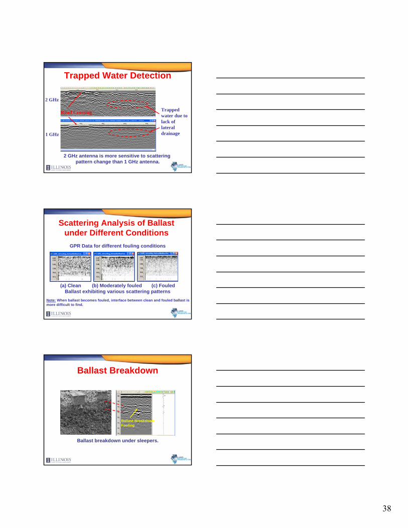
Trapped Water Detection

Trapped water due to lack of lateral drainage

Road Crossing

2 GHz antenna is more sensitive to scattering pattern change than 1 GHz antenna.

2 GHz

1 GHz

Scattering Analysis of Ballast under Different Conditions

Threshold Image

(a) Clean (b) Moderately fouled (c) Fouled Ballast exhibiting various scattering patterns

GPR Data for different fouling conditions

Note: When ballast becomes fouled, interface between clean and fouled ballast is more difficult to find.

Ballast Breakdown

Ballast breakdown under sleepers.

Ballast BreakdownFouling

39

Summary• GPR is a NDE technique that can be

used effectively to evaluate various transportation structures

• GPR can provide quick and reliable information about the subsurface.

• GPR reliable applications include:– Layer thickness estimation– Subsurface Moisture/ Distress detection– Rebar cover depth estimation– Rail Road evaluation (Ballast)– …

Thank You!

Questions?