Geometric Brownian Motion

Note that as a model for the rate of return, dS(t)/S(t) geometric

Brownian motion is similar to other common statistical models:

dS(t)

S(t)= µdt + σdW (t)

or

response = systematic component + random error.

Without the stochastic component, the differential equation has

the simple solution

S(t) = ceµt,

from which we get the formula for continuous compounding for

a rate µ.

1

An Intuitive Examination of Geometric

Brownian Motion in Prices

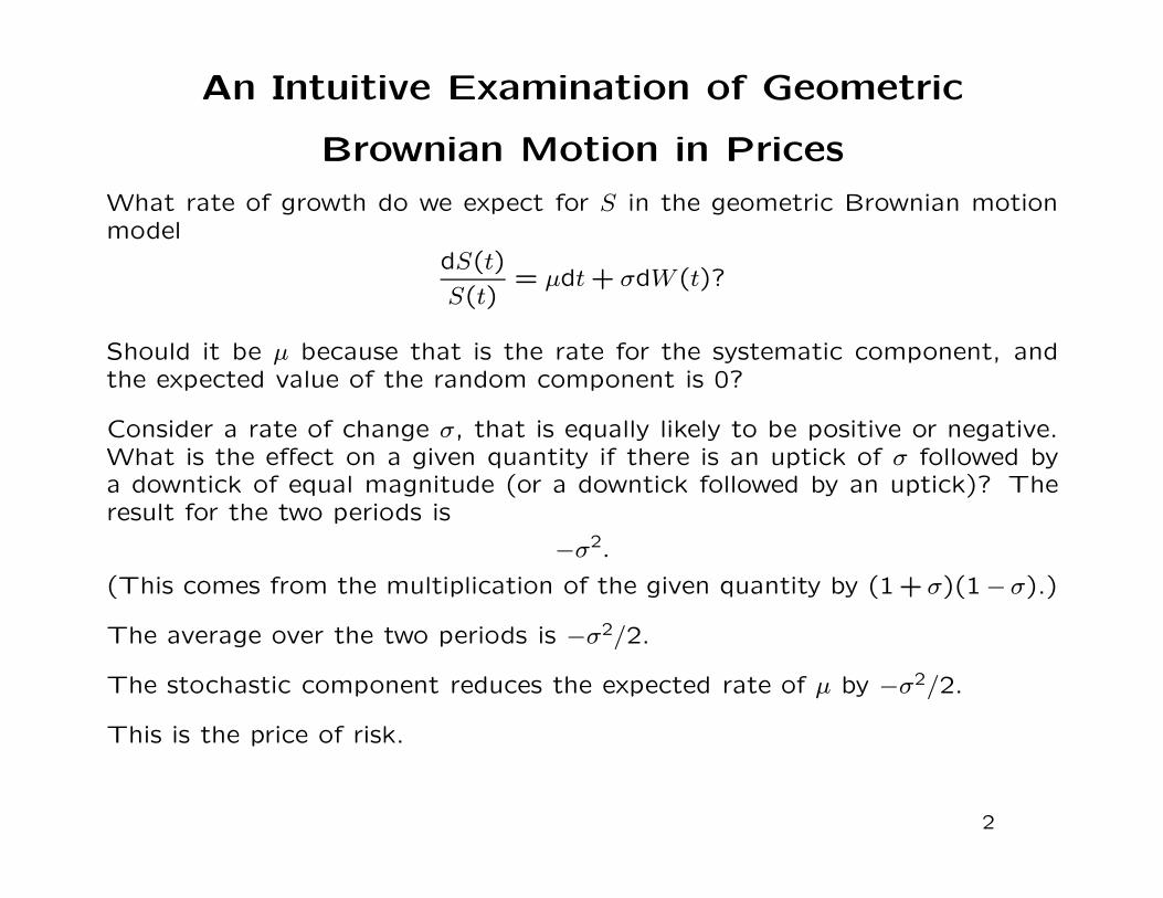
What rate of growth do we expect for S in the geometric Brownian motionmodel

dS(t)

S(t)= µdt + σdW(t)?

Should it be µ because that is the rate for the systematic component, andthe expected value of the random component is 0?

Consider a rate of change σ, that is equally likely to be positive or negative.What is the effect on a given quantity if there is an uptick of σ followed bya downtick of equal magnitude (or a downtick followed by an uptick)? Theresult for the two periods is

−σ2.

(This comes from the multiplication of the given quantity by (1+ σ)(1−σ).)

The average over the two periods is −σ2/2.

The stochastic component reduces the expected rate of µ by −σ2/2.

This is the price of risk.

2

Ito’s Lemma

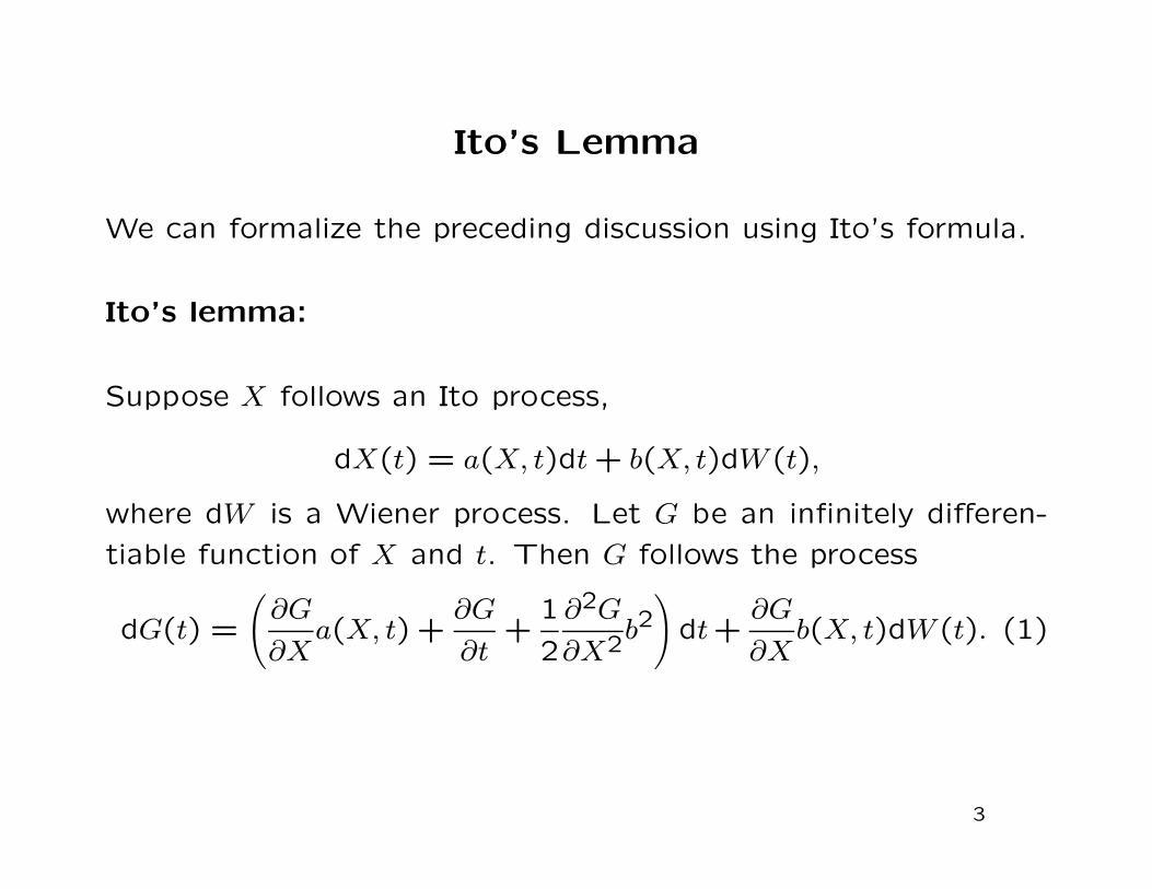
We can formalize the preceding discussion using Ito’s formula.

Ito’s lemma:

Suppose X follows an Ito process,

dX(t) = a(X, t)dt + b(X, t)dW (t),

where dW is a Wiener process. Let G be an infinitely differen-

tiable function of X and t. Then G follows the process

dG(t) =

(

∂G

∂Xa(X, t) +

∂G

∂t+

1

2

∂2G

∂X2b2)

dt+∂G

∂Xb(X, t)dW (t). (1)

3

Ito’s Lemma

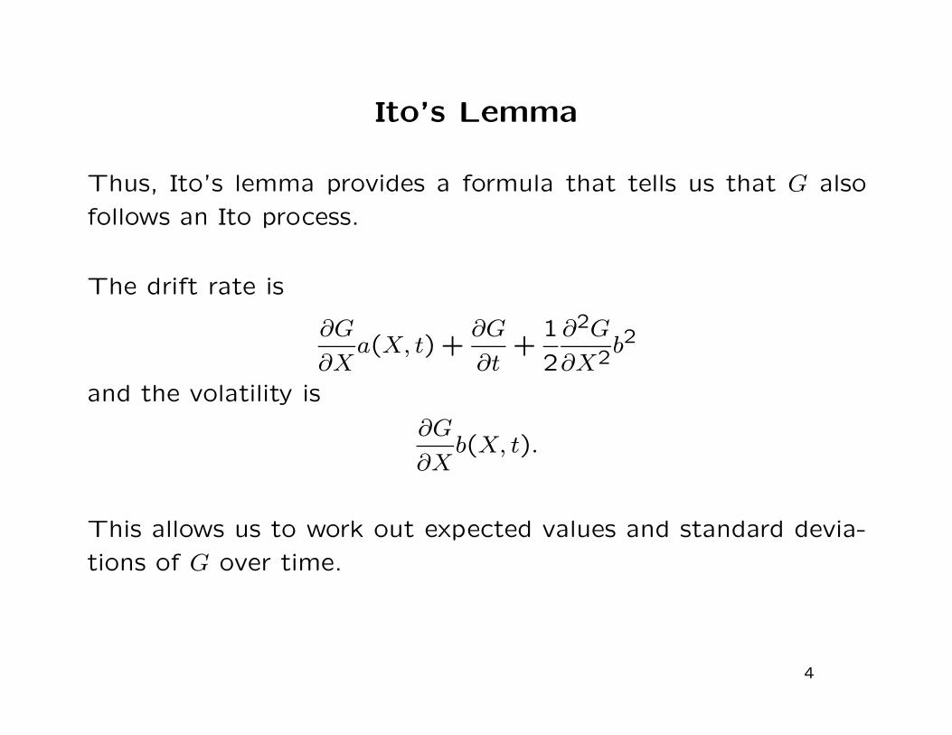
Thus, Ito’s lemma provides a formula that tells us that G also

follows an Ito process.

The drift rate is

∂G

∂Xa(X, t) +

∂G

∂t+

1

2

∂2G

∂X2b2

and the volatility is

∂G

∂Xb(X, t).

This allows us to work out expected values and standard devia-

tions of G over time.

4

Derivation of Ito’s Formula

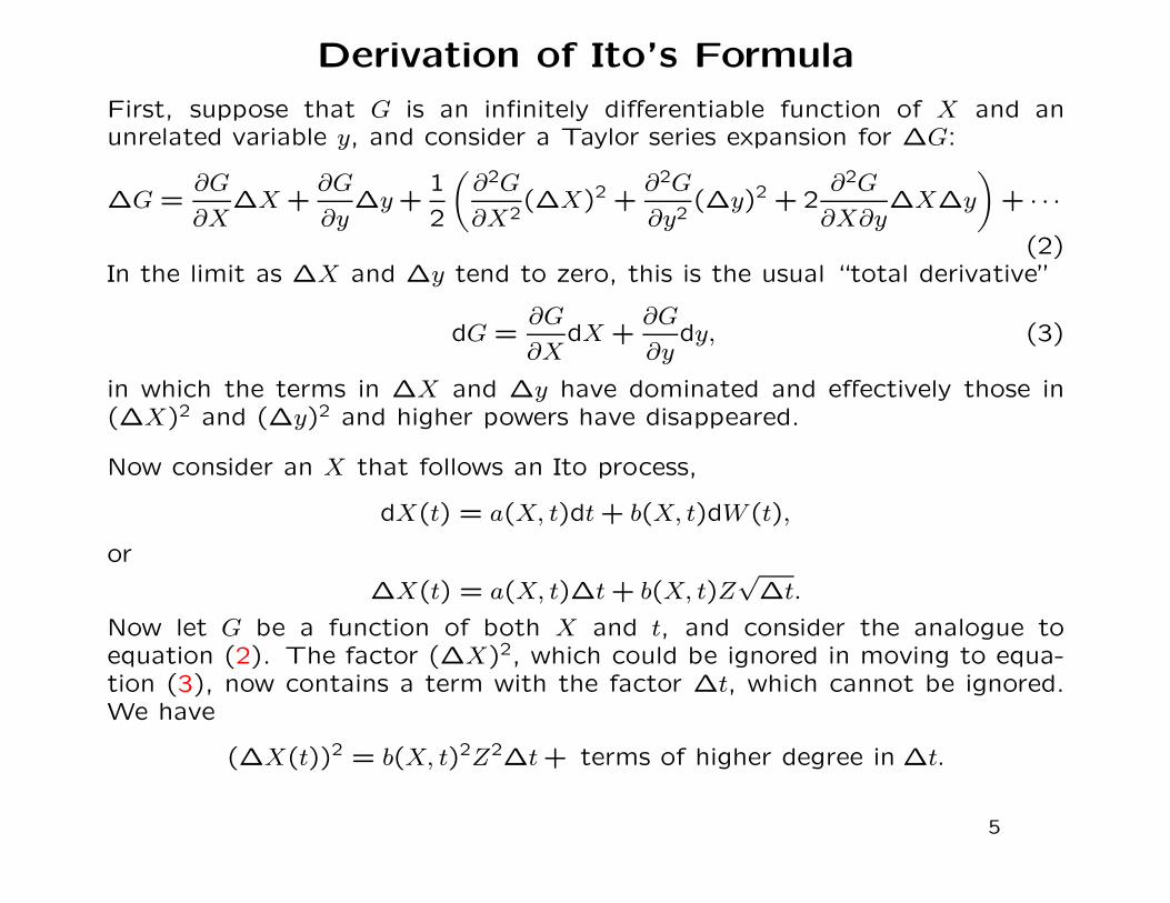
First, suppose that G is an infinitely differentiable function of X and anunrelated variable y, and consider a Taylor series expansion for ∆G:

∆G =∂G

∂X∆X +

∂G

∂y∆y +

1

2

(

∂2G

∂X2(∆X)2 +

∂2G

∂y2(∆y)2 + 2

∂2G

∂X∂y∆X∆y

)

+ · · ·

(2)In the limit as ∆X and ∆y tend to zero, this is the usual “total derivative”

dG =∂G

∂XdX +

∂G

∂ydy, (3)

in which the terms in ∆X and ∆y have dominated and effectively those in(∆X)2 and (∆y)2 and higher powers have disappeared.

Now consider an X that follows an Ito process,

dX(t) = a(X, t)dt + b(X, t)dW(t),

or

∆X(t) = a(X, t)∆t + b(X, t)Z√

∆t.

Now let G be a function of both X and t, and consider the analogue toequation (2). The factor (∆X)2, which could be ignored in moving to equa-tion (3), now contains a term with the factor ∆t, which cannot be ignored.We have

(∆X(t))2 = b(X, t)2Z2∆t + terms of higher degree in ∆t.

5

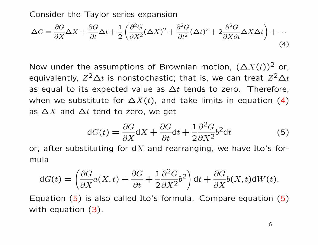
Consider the Taylor series expansion

∆G =∂G

∂X∆X +

∂G

∂t∆t +

1

2

(

∂2G

∂X2(∆X)2 +

∂2G

∂t2(∆t)2 + 2

∂2G

∂X∂t∆X∆t

)

+ · · ·

(4)

Now under the assumptions of Brownian motion, (∆X(t))2 or,

equivalently, Z2∆t is nonstochastic; that is, we can treat Z2∆t

as equal to its expected value as ∆t tends to zero. Therefore,

when we substitute for ∆X(t), and take limits in equation (4)

as ∆X and ∆t tend to zero, we get

dG(t) =∂G

∂XdX +

∂G

∂tdt +

1

2

∂2G

∂X2b2dt (5)

or, after substituting for dX and rearranging, we have Ito’s for-

mula

dG(t) =

(

∂G

∂Xa(X, t) +

∂G

∂t+

1

2

∂2G

∂X2b2)

dt +∂G

∂Xb(X, t)dW (t).

Equation (5) is also called Ito’s formula. Compare equation (5)

with equation (3).

6

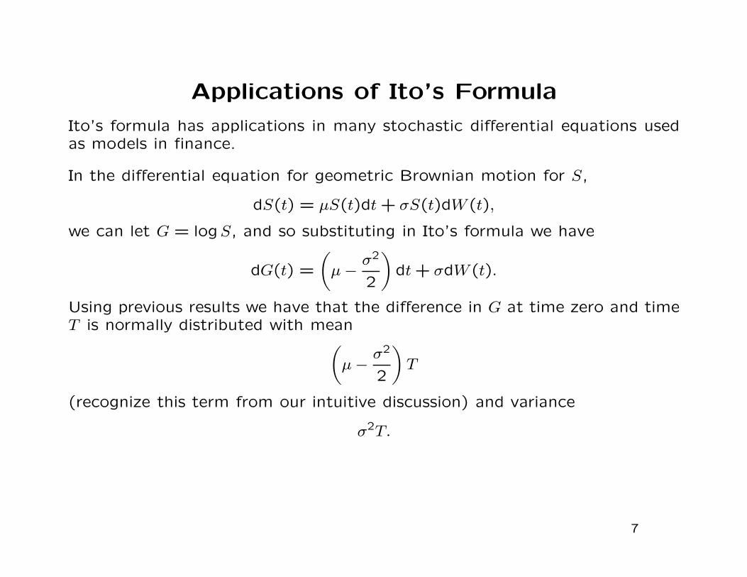
Applications of Ito’s Formula

Ito’s formula has applications in many stochastic differential equations usedas models in finance.

In the differential equation for geometric Brownian motion for S,

dS(t) = µS(t)dt + σS(t)dW(t),

we can let G = logS, and so substituting in Ito’s formula we have

dG(t) =

(

µ − σ2

2

)

dt + σdW(t).

Using previous results we have that the difference in G at time zero and timeT is normally distributed with mean

(

µ − σ2

2

)

T

(recognize this term from our intuitive discussion) and variance

σ2T.

7

The Distribution of Stock Prices

The geometric Brownian motion model is the simplest model

for stock prices that is somewhat realistic. Looking at it some-

what critically, we can see certain problems. First, is the form

of the differential equation reasonable? Next, we have the big

questions: are µ and σ constant? We will explore these issues

later.

The basic distributional assumption in the geometric Brownian

motion model is that the rates of change of stock prices in very

small increments of time are identically and independently nor-

mally distributed.

8

The Distribution of Stock Prices

The compounded rate of return is

1

∆tlog(S(t + ∆t)/S(t)).

From t0 to T we can write this as

1

T − t0log(ST )− 1

T − t0log(St0).

If this has a normal distribution, then log(ST ) has a normal dis-

tribution; that is, ST has a lognormal distribution.

*** properties

9

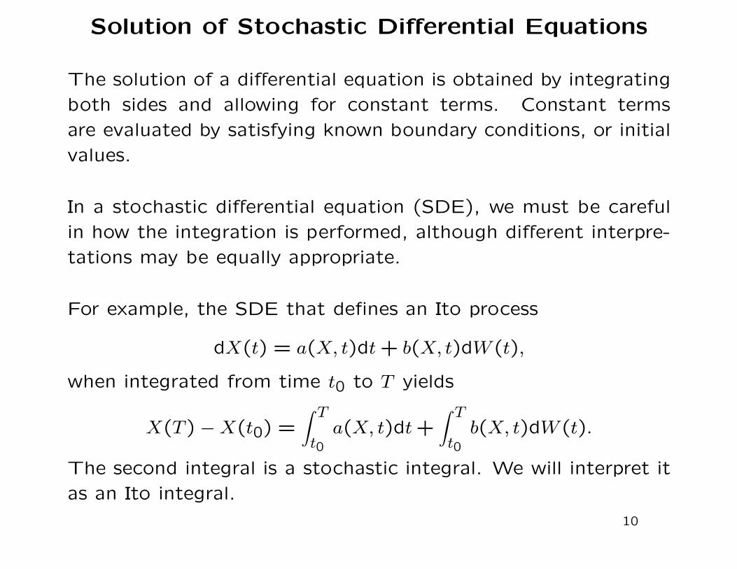
Solution of Stochastic Differential Equations

The solution of a differential equation is obtained by integrating

both sides and allowing for constant terms. Constant terms

are evaluated by satisfying known boundary conditions, or initial

values.

In a stochastic differential equation (SDE), we must be careful

in how the integration is performed, although different interpre-

tations may be equally appropriate.

For example, the SDE that defines an Ito process

dX(t) = a(X, t)dt + b(X, t)dW (t),

when integrated from time t0 to T yields

X(T) − X(t0) =∫ T

t0a(X, t)dt +

∫ T

t0b(X, t)dW (t).

The second integral is a stochastic integral. We will interpret it

as an Ito integral.

10

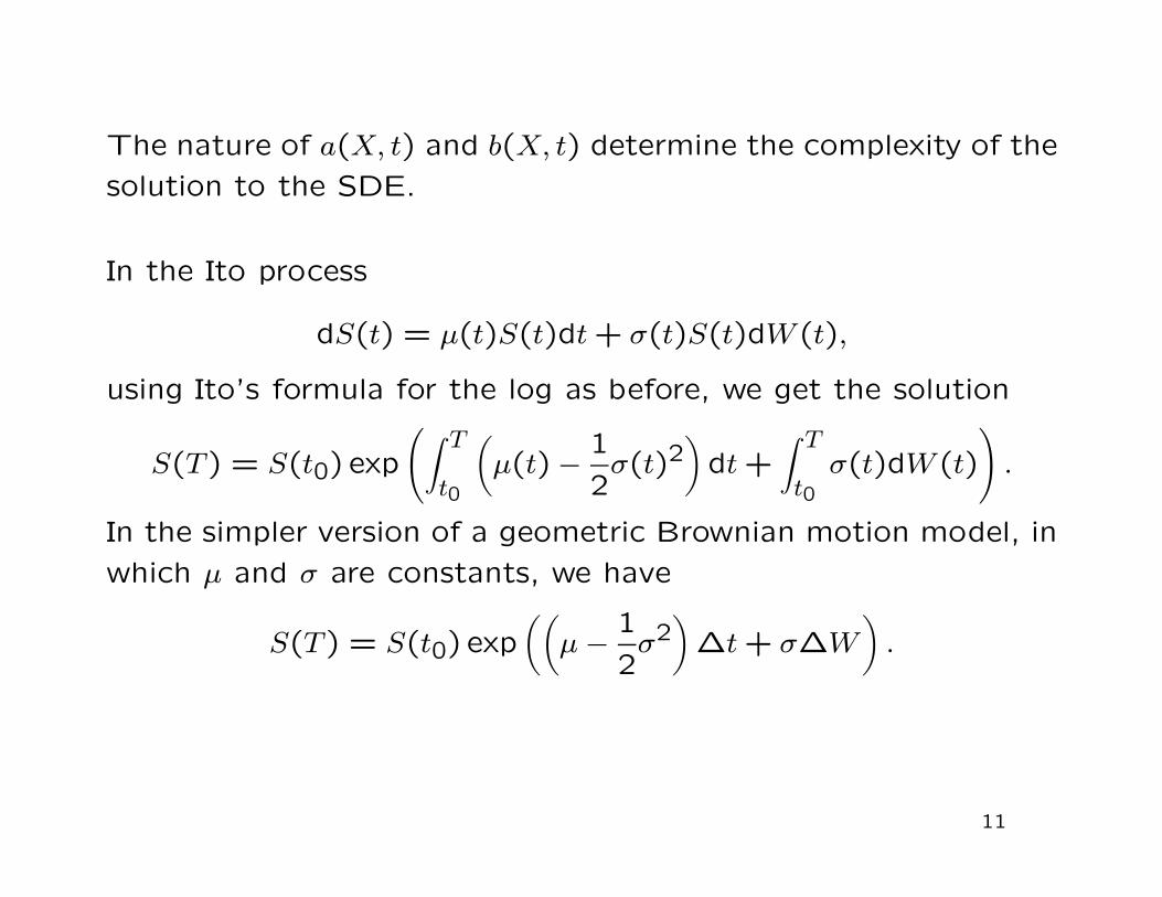
The nature of a(X, t) and b(X, t) determine the complexity of the

solution to the SDE.

In the Ito process

dS(t) = µ(t)S(t)dt + σ(t)S(t)dW (t),

using Ito’s formula for the log as before, we get the solution

S(T) = S(t0) exp

(

∫ T

t0

(

µ(t)− 1

2σ(t)2

)

dt +∫ T

t0σ(t)dW (t)

)

.

In the simpler version of a geometric Brownian motion model, in

which µ and σ are constants, we have

S(T) = S(t0) exp

((

µ − 1

2σ2)

∆t + σ∆W)

.

11

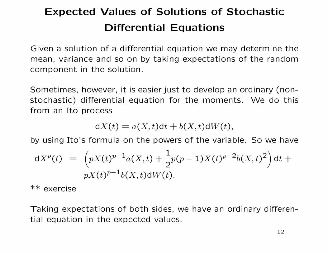
Expected Values of Solutions of Stochastic

Differential Equations

Given a solution of a differential equation we may determine the

mean, variance and so on by taking expectations of the random

component in the solution.

Sometimes, however, it is easier just to develop an ordinary (non-

stochastic) differential equation for the moments. We do this

from an Ito process

dX(t) = a(X, t)dt + b(X, t)dW (t),

by using Ito’s formula on the powers of the variable. So we have

dXp(t) =

(

pX(t)p−1a(X, t) +1

2p(p − 1)X(t)p−2b(X, t)2

)

dt +

pX(t)p−1b(X, t)dW (t).

** exercise

Taking expectations of both sides, we have an ordinary differen-

tial equation in the expected values.

12

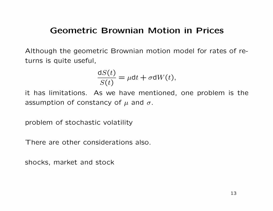
Geometric Brownian Motion in Prices

Although the geometric Brownian motion model for rates of re-

turns is quite useful,

dS(t)

S(t)= µdt + σdW (t),

it has limitations. As we have mentioned, one problem is the

assumption of constancy of µ and σ.

problem of stochastic volatility

There are other considerations also.

shocks, market and stock

13

Derivatives: Basics

A derivative is a financial instrument whose value depends on

values of other financial instruments or on some measure of the

state of the economy or of nature. The instrument or measure

on whose value the derivative depends is called the “underlying”.

A derivative is an agreement with two sides.

One of the most important questions in finance is how to price

a derivative.

14

Forward Contracts

One of the simplest kinds of derivatives is a forward contract,

which is an agreement to buy or to sell an asset at a specified

time at a specified price.

The agreement to buy is a long position and the agreement to

sell is a short position. The agreed upon price is the delivery

price. The consumation of the agreement is an execution.

Forward contracts are relatively simple to price, and their analysis

is important for developing pricing methods for other derivatives.

15

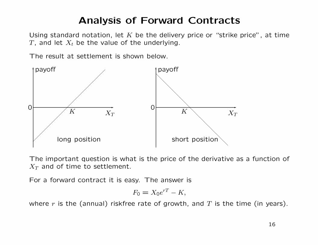
Analysis of Forward Contracts

Using standard notation, let K be the delivery price or “strike price”, at timeT , and let Xt be the value of the underlying.

The result at settlement is shown below.

payoff6

XTK

long position

0 -

��

��

��

��

��

��

��

��

�� payoff6

XTK

short position

0 -

@@

@@

@@

@@

@@

@@

@@

@@

@@

The important question is what is the price of the derivative as a function ofXT and of time to settlement.

For a forward contract it is easy. The answer is

F0 = X0erT − K,

where r is the (annual) riskfree rate of growth, and T is the time (in years).

16

Derivatives: Basics

There is a variety of modifications to the basic forward contract

that involve

• nature of the underlying

– asset

∗ investment

∗ consumable

∗ income producing

– nonasset (e.g., index, price of electricity, weather)

• negociability of the instrument (market, possibility of short

positions, intermediate party, etc.)

17

Derivatives: Basics

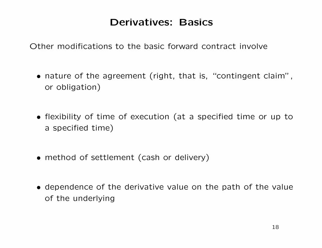
Other modifications to the basic forward contract involve

• nature of the agreement (right, that is, “contingent claim”,

or obligation)

• flexibility of time of execution (at a specified time or up to

a specified time)

• method of settlement (cash or delivery)

• dependence of the derivative value on the path of the value

of the underlying

18

Types of Derivatives

These variations on the basic forward contract are all interesting. Only a fewof them are actually available.

Some variations are much easier to analyze than others. The simple ones areinteresting for classroom analyses and they may provide useful approximationsfor derivatives that are actually available.

For individual investors, there is a relatively small set of derivatives available(realistically).

For all of them there is a ready market (always) through a third party, andshort sales are possible.

Most of the readily traded derivatives are options, or contingent claims. Thatkind of derivative is a right; not an obligation.

Therefore, a long position is a right and a short position (in the derivative)is an obligation. The right “expires” at the settlement date.

19

Derivatives That Have Markets

The common types of derivatives are

• Stock options

• Index options

• Commodity futures

• Rate futures

20

Uses

Stock options are used by individual investors and by investment

companies for leverage, hedging, and income.

Index options are used by individual investors and by investment

companies for hedging and speculative income.

Commodity futures are used by individual investors for specula-

tive income, by investment companies for income, and by pro-

ducers and traders for hedging.

Rate futures are used by individual investors for speculative in-

come, by investment companies for income and for hedgins, and

by traders for hedging.

21

Types of Common Derivatives

The variations depend on the nature of the underlying.

• Stock (investment asset, possibly income-producing). The buy side is a“call” and the sell side is a “put”.

– Settlement (exercise) is by delivery.

– Exercise can be any time prior to expiration date (“American style”).

• Index (investment asset, not income-producing). The buy side is a “call”and the sell side is a “put”.

– Settlement is by cash.

– Exercise can only be at expiration date.

• Commodity (consumable asset, not income-producing).

– Settlement is by delivery.

– Exercise can only be at expiration date.

22

U.S. Stock Options

A market for stock options in the U.S. is one of the national

security exchanges: Amex, CBOE, NYSE, Pacific Exchange, and

Philadelphia Exchange.

All (almost all) options are initiated with and through the Op-

tions Clearing Corporation, owned by the exchanges and head-

quartered on LaSalle St.

Options (and also futures) are regulated by the Commodity Fu-

tures Trading Commission (the analogue of the SEC). The SEC

also regulates options through its regulatory oversight of the

exchanges.

23

Analysis of Stock Options

Another important difference between stock options and forward

contracts is that stock options are rights, not obligations. The

payoff therefore cannot be negative.

Because the payoff cannot be negative, there must be a cost to

obtain a stock option.

The profit is the difference between the payoff and the price paid.

Another difference in stock options and forward contracts is that

(real-world) stock options can be exercised at any time (during

trading hours) prior to expiration. We will, however, often con-

sider a modification, the “European option”, which can only be

exercised at a specified time. (There are some European op-

tions that are actually traded, but they are generally for large

amounts, and they are rarely traded by individuals.)

24

Analysis of Stock Options

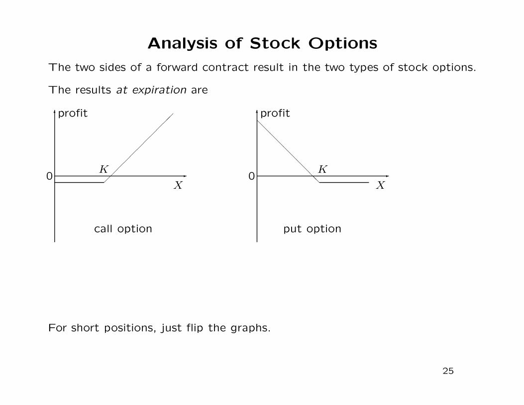
The two sides of a forward contract result in the two types of stock options.

The results at expiration are

profit6

X

K

call option

0 -�

��

��

��

��

�� profit6

X

K

put option

0 -

@@

@@

@@

@@

@@

For short positions, just flip the graphs.

25

Market Models for Derivative Pricing

A simple model of the market assumes two assets:

a riskless asset with price at time t of βt,

and a risky asset with price at time t of Xt.

The price of a derivative can be determined based on trading

strategies involving these two assets.

The price of the riskless asset follows the deterministic ordinary

differential equation

dβt = rβtdt,

where r is the instantaneous riskfree interest rate.

The price of the risky asset follows the stochastic differential

equation

dXt = µXtdt + σXtdWt.

26

Pricing Derivatives: Basics

Start with a European call option. How do we value it?

Current time: t0

Expiration: T

Strike price: K

Price of underlying: S(t0), . . . , S(t), . . . , S(T)

Value of the call: C(t0), . . . , C(t), . . . , C(T)

P for put; V for either

We have been (and in this course will continue to be) vague

about the pricing unit. In general, we call the price, or the

pricing unit, a numeraire. A more careful development of this

concept rests on the idea of a pricing kernel.

We will usually call them dollars.

27

The Price of a European Call Option

A European call option is a contract that gives the owner the

right to buy a specified amount of an underlying for a fixed strike

price, K on the expiration or maturity date T .

The owner of the option does not have any obligations in the

contract.

The payoff, h, of the option at time T is either 0 or the excess

of the price of the underlying S(T) over the strike price K.

Once the parameters K and T are set, it is a function of S(T):

h(S(T)) =

{

S(T) − K if S(T) > K0 otherwise

28

The Price of Call Options

The price of the option at any time is a function of the time t,

and the price of the underlying s. We denote it as P (t, s).

What is the price at time t = 0?

It seems natural that the price of the European call option should

be the expected value of the payoff of the option at expiration,

discounted back to t = 0:

P (0, s) = e−rTE(h(S(T))).

Likewise, for an American option, we could maximize the ex-

pected value over all stopping times, 0 < τ < T :

P (0, s) = supτ≤T

e−rτE(h(S(τ))).

29

Principles

Basic principle of Black-Scholes: We seek a portfolio with zero

expected value, that consists of short and/or long positions in

the option, the underlying, and a risk-free bond.

There are two key ideas in developing pricing formulas for deriva-

tives:

1. no-arbitrage principle

2. replicating, or hedging, portfolio

30

An arbitrage is a trading strategy with a guaranteed rate of return

that exceeds the riskless rate of return.

In financial analysis, we assume that arbitrages do not exist.

31

Example of the No-Arbitrage Principle

Consider a forward contract that obligates one to pay K at T for the under-lying. At time t, with t < T , the price of the underlying is S(t). What shouldthe price of the contract be or, equivalently,

What should K be so that the price of the contract is 0?

Its value at expiry is S(T )−K, and of course we do not know S(T ). If we havea riskless rate of return r, we can use the no-arbitrage principle to determinethe correct price of the contract.

To apply the no-arbitrage principle, consider the following strategy:

take a long position in the forward contract andsell the underlying short.

With this strategy, the investor immediately receives S(t). At time T thisamount can be guaranteed to be

S(t)er(T−t).

32

The No-Arbitrage Principle

If

K < S(t)er(T−t),

a long position in the forward contract and

a short position in the underlying

is an arbitrage.

Conversely, if

K > S(t)er(T−t),

a short position in the forward contract and

a long position in the underlying

is an arbitrage.

Therefore, under the no-arbitrage assumption, the correct value

of K is S(t)er(T−t).

33

The replication approach is to determine a portfolio and an asso-

ciated trading strategy that will provide a payout that is identical

to that of the underlying. This portfolio and trading strategy

replicates the derivative.

A replicating strategy involves both long and short positions.

34

Pricing Derivatives

If every derivative can be replicated by positions in the underlying

(and cash), the economy or market is said to be complete.

We will generally assume complete markets.

The Black-Scholes approach leads to the idea of a self-financing

replicating hedging strategy.

The approach yields the interesting fact that the price of the call

does not depend on the expected value of the underlying.

It does depend on its volatility, however.

35

Self-Financing Replicating Hedging Strategy

Neil Chriss’s example of a casino.

Game is to flip a fair coin 3 times.

Casino pays $1 if heads occurs 3 times in a row, HHH.

How much should it cost to play? (Casino will then add operating

and profit margin.)

Relation to options; who’s short and who’s long

Big player: $100,000.

Bet broker: casino bets $12,500 on H on first toss; casino is

even

If H occurs, casino has $25,000 and bets on H on second toss

36

Analysis of Casino Hedging Example

Hedging – in general

Special properties:

Self-financing

Replicating.

Roles of three participants; who’s short and who’s long

bid-ask spread (will broker charge the expected value of the bet?)

other transaction costs...

Assumptions: market impact, complete market

37

Expected Rate of Return on Stock

XYZ selling at S(t0); no dividends.

What is its expected value at time T > t0?

It is merely the forward price for what it could be bought now.

Forward price: er(T−t0)S(t0),

where r is the risk-free rate of return, S(t0) is the spot price,

and T − t0 is the time interval.

This is the no-arbitrage principle.

The expected value of the stock does not depend on the

rate of return of the stock

(that’s µ in some of the models we’ve used).

This is true because of the cost of a forward contract.

38

Call Option

Holder of the forward contract (long position) on XYZ must buy

stock at time T for er(T−t0)S(t0).

Holder of a call option buys stock only if S(T) > K.

Role of volatility

on forward contract holder (volatility not good)

on call option holder (volatility good) – enhances the value of

the option

Assumptions ...

Conclusion under assumptions: expected volatility of the under-

lying affects the value of an option, but expected rate of return

of the underlying does not.

39

Hedging

Hedging risk: defray the risk of one investment by making an

offsetting investment.

Cost of hedge.

Return of hedge (reduced risk).

Perfect hedge: returns exactly the amount needed to cover any

loss, and no more.

Example: write call (i.e., go short). what is a hedge? own-

ing enough stock to cover is a hedge, but not perfect (it costs

too much, and writer is not protected against drop in price of

underlying).

40

Hedging

Black-Scholes approach constructs a portfolio consisting of some

underlying and some risk-free (zero-coupon) bonds to offset the

short call.

(discuss dividends, coupons, etc.)

41

Hedging

In a perfect hedge, the hedging instrument behaves exactly the

way the hedged instrument does.

Call option vs. hedging instrument: value at T .

they’re equal ... called “payoff replication”.

42

Dynamic Hedging

process of managing the risk of options

hedging portfolio’s value at any time is equal to the value of the

option at that point in time.

1. replicates the payoff

2. has fixed and known total cost

weighted portfolio, balancing

hedging strategy produces a synthetic version of the option.

43

Self-Financing Dynamic Hedging

Cost of hedge:

1. infusion of funds cost

2. transaction costs (bid-ask, friction, inability to execute trades

at exactly the price specified by the strategy, etc.)

A hedging strategy is self-financing if its total to-date cost at

any time (excluding transaction costs) is equal to the setup cost.

Setup cost: initial outlay; e.q. strategy requires going long

$1,000 and short $700; setup is $300

To do this, we need a formula for the relative rates of change of

the price of the call and that of the underlying,

∆ =dC

dS.

44

Delta of an Option

The delta of an option is the rate of change of the option’s value

with respect to the change in the underlying’s price.

Consider times t0 and t1. If the value of an option at time t is

V (t), and the price of the underlying is S(t), the delta at t0 is

approximated by

∆t0 =V (t0)− e−r(t1−t0)V (t1)

S(t0)− e−r(t1−t0)S(t1).

We essentially neutralize the change in time by the risk-free rate.

comments: zero in denominator; time value

45

Market Models for Derivative Pricing

A simple model of the market assumes two assets:

a riskless asset with price at time t of βt,

and a risky asset with price at time t of S(t).

The price of a derivative can be determined based on trading

strategies involving these two assets.

The price of the riskless asset follows the deterministic ordinary

differential equation

dβt = rβtdt,

where r is the instantaneous riskfree interest rate.

The price of the risky asset follows the stochastic differential

equation

dS(t) = µS(t)dt + σS(t)dWt.

46

Preliminary Formula

C(t) = ∆tS(t) − er(T−t)B(t),

where B(t) is the current value of a riskless bond.

47

We speak of a portfolio as a vector p whose elements sum to 1.

The length of the vector is the number of assets in our universe.

Sometimes we limit this to assets whose values are independent

of each other; that is, we may exclude derivatives.

The no-arbitrage principle can be stated as:

There does not exist a p such that for some t > 0, either

• pTs0 < 0 and pTS(t)(ω) ≥ 0 for all ω,

or

• pTs0 ≤ 0 and pTS(t)(ω) ≥ 0 for all ω, and pTS(t)(ω) > 0 for

some ω.

48

A derivative D is said to be attainable (over a universe of assets

S = (S(1), S(2), . . . , S(k))) if there exists a portfolio p such that

for all ω and t,

Dt(ω) = pTS(t)(ω).

Not all derivatives are attainable. The replicating portfolio ap-

proach to pricing derivatives applies only to those that are at-

tainable.

49

Dynamic and Self-Financing Portfolios

The value of a derivative changes in time and as a function of the

value of the underlying; therefore, a replicating portfolio must be

changing in time or “dynamic”.

In analyses with replicating portfolios, transaction costs are ig-

nored.

Also, the replicating portfolio must be self-financing; that is,

once the portfolio is initiated, no further capital is required. Ev-

ery purchase is financed by a sale.

50

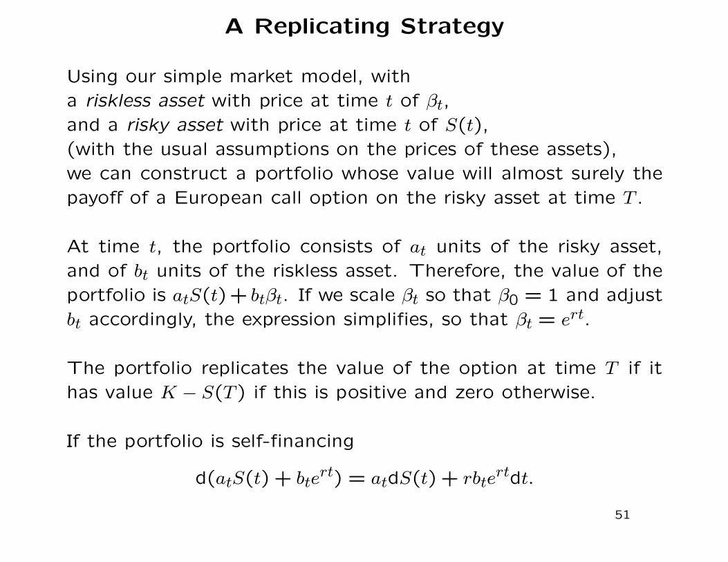
A Replicating Strategy

Using our simple market model, with

a riskless asset with price at time t of βt,

and a risky asset with price at time t of S(t),

(with the usual assumptions on the prices of these assets),

we can construct a portfolio whose value will almost surely the

payoff of a European call option on the risky asset at time T .

At time t, the portfolio consists of at units of the risky asset,

and of bt units of the riskless asset. Therefore, the value of the

portfolio is atS(t)+ btβt. If we scale βt so that β0 = 1 and adjust

bt accordingly, the expression simplifies, so that βt = ert.

The portfolio replicates the value of the option at time T if it

has value K − S(T) if this is positive and zero otherwise.

If the portfolio is self-financing

d(atS(t) + btert) = atdS(t) + rbte

rtdt.

51

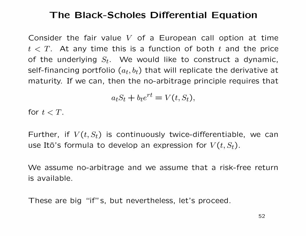
The Black-Scholes Differential Equation

Consider the fair value V of a European call option at time

t < T . At any time this is a function of both t and the price

of the underlying St. We would like to construct a dynamic,

self-financing portfolio (at, bt) that will replicate the derivative at

maturity. If we can, then the no-arbitrage principle requires that

atSt + btert = V (t, St),

for t < T .

Further, if V (t, St) is continuously twice-differentiable, we can

use Ito’s formula to develop an expression for V (t, St).

We assume no-arbitrage and we assume that a risk-free return

is available.

These are big “if”s, but nevertheless, let’s proceed.

52

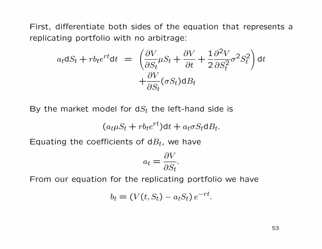
First, differentiate both sides of the equation that represents a

replicating portfolio with no arbitrage:

atdSt + rbtertdt =

(

∂V

∂StµSt +

∂V

∂t+

1

2

∂2V

∂S2t

σ2S2t

)

dt

+∂V

∂St(σSt)dBt

By the market model for dSt the left-hand side is

(atµSt + rbtert)dt + atσStdBt.

Equating the coefficients of dBt, we have

at =∂V

∂St.

From our equation for the replicating portfolio we have

bt = (V (t, St)− atSt) e−rt.

53

Now, equating coefficients of dt and substituting for at and bt,

we have the Black-Scholes differential equation,

r

(

V − St∂V

∂St

)

=∂V

∂t+

1

2σ2S2

t∂2V

∂S2t

Notice that µ is not in the equation.

54

Delta Hedging

The Black-Scholes differential equation can also be derived by

constructing a riskless, self-financing portfolio consisting of a

long position in the underlying and a short position in the call.

Letting At be the amount long in the underlying, and Nt be the

amount short in the derivative, we arrive at the equation

At

Nt=

∂V

∂St.

The ratio AtNt

is called the Delta, and this approach to riskless

portfolio construction is called delta hedging.

55

The Black-Scholes Differential Equation

Instead of European calls, we can consider European puts, and

proceed in the same ways (replicating portfolio or Delta hedging).

We arrive at the same the Black-Scholes differential equation

(rewritten),

∂V

∂t+ rSt

∂V

∂St+

1

2σ2S2

t∂2V

∂S2t

= rV.

56

The Black-Scholes Formula

The solution depends on the boundary conditions. In the case

of European options, these are simple.

For calls, they are

Vc(T, St) = (St − K)+

For puts, they are

Vp(T, St) = (K − St)+

57

The Black-Scholes Formula

With these boundary conditions, there are closed form solutions

to the Black-Scholes differential equation.

For the call, it is

CBS(t, St) = StΦ(d1) − Ke−r(T−t)Φ(d2),

where

d1 =log(St/K) + (r + 1

2σ2)(T − t)

σ√

T − t,

d2 = d1 − σ√

T − t,

and

Φ(s) =1√2π

∫ s

−∞e−y2/2dy.

58

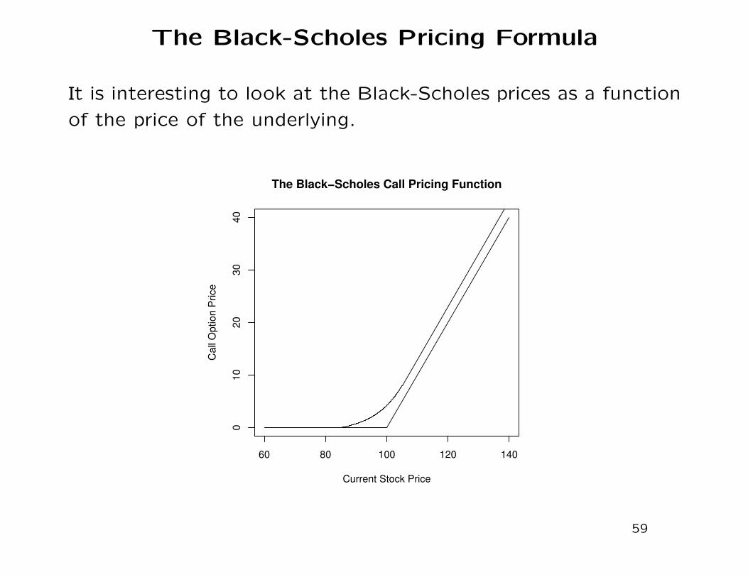
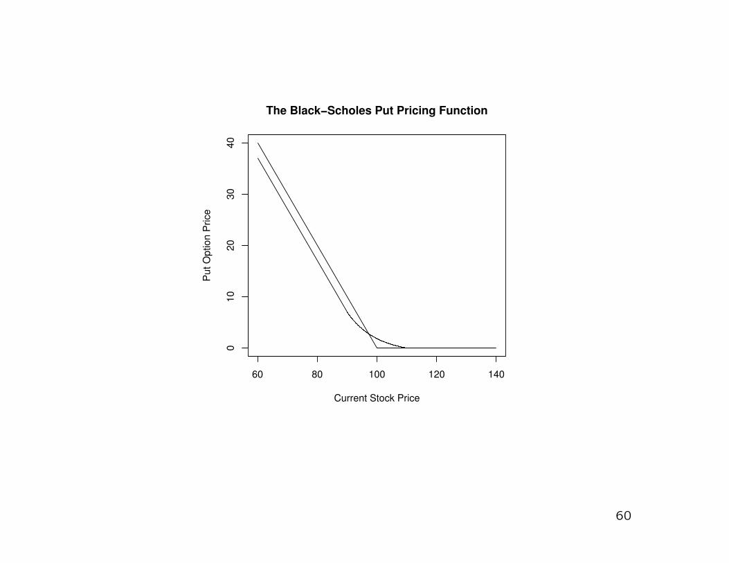
The Black-Scholes Pricing Formula

It is interesting to look at the Black-Scholes prices as a function

of the price of the underlying.

60 80 100 120 140

010

20

30

40

Current Stock Price

Call

Option P

rice

The Black−Scholes Call Pricing Function

59

60 80 100 120 140

010

20

30

40

Current Stock Price

Put O

ption P

rice

The Black−Scholes Put Pricing Function

60

Assumptions

The Black-Scholes model depends on several assumptions:

• differentiability of stock prices with respect to time

• a dynamic replicating portfolio can be maintained without

transaction costs

• returns are

· independent

· normal

· mean stationary

· variance stationary

61

Stochastic Volatility

A condition in which the variance of the returns is random (rather

than stationary) is called “stochastic volatility”.

Data on returns provide empirical evidence that the volatility is

stochastic.

62

Stochastic Volatility and Implied Volatility

Stochastic volatility can also account for other empirically ob-

served failures of the Black-Scholes model.

For a given option (underlying, type, strike price, and expiry)

and given the price of the underlying and the riskfree rate, the

Black-Scholes formula relates the option price to the volatility

of the underlying; that is, the volatility determines the model

option price.

The actual price at which the option trades can be observed,

however.

If this price is used in the Black-Scholes formula, the volatility

can be computed. This is called the “implied volatility”.

63

Implied Volatility

Recall the Black-Scholes formula:

CBS(t, St) = StΦ(d1) − Ke−r(T−t)Φ(d2),

where

d1 =log(St/K) + (r + 1

2σ2)(T − t)

σ√

T − t,

d2 = d1 − σ√

T − t,

as before.

Let c be the observed price of the call. Now, set CBS(t, St) = c,

and

f(σ) = StΦ(d1)− Ke−r(T−t)Φ(d2),

We have

c = f(σ).

64

Computing the Implied Volatility

Given a value for c, that is, the observed price of the option, we

can solve for σ. There is no closed-form solution, so we solve

iteratively. Beginning with σ(0), we can use the Newton updates,

σ(k+1) = σ(k) − (f(σ(k)) − c)/f ′(σ(k)).

65

Computing the Implied Volatility

We have

f ′(σ) = StdΦ(d1)

dσ− Ke−r(T−t)dΦ(d2)

dσ

= Stφ(d1)dd1

dσ− Ke−r(T−t)φ(d2)

dd2

dσ,

where

φ(y) =1√2π

e−y2/2,

dd1

dσ=

σ2(T − t) − log(St/K)− (r + 12σ2)(T − t)

σ2√

T − t,

and

dd2

dσ=

dd1

dσ−

√T − t.

66

Discrepancies in the Observed Implied

Volatilities

The implied volatility from the Black-Scholes model should be

the same at all points. It is not.

The implied volatility, for given T and St, depends on the strike

price, K.

In general, the implied volatility is greater than the empirical

volatility, but the implied volatility is even greater for far out-of-

the money calls. It also increases for deep in-the-money calls.

This is called the “smile curve”, or the “volatility smile”.

67

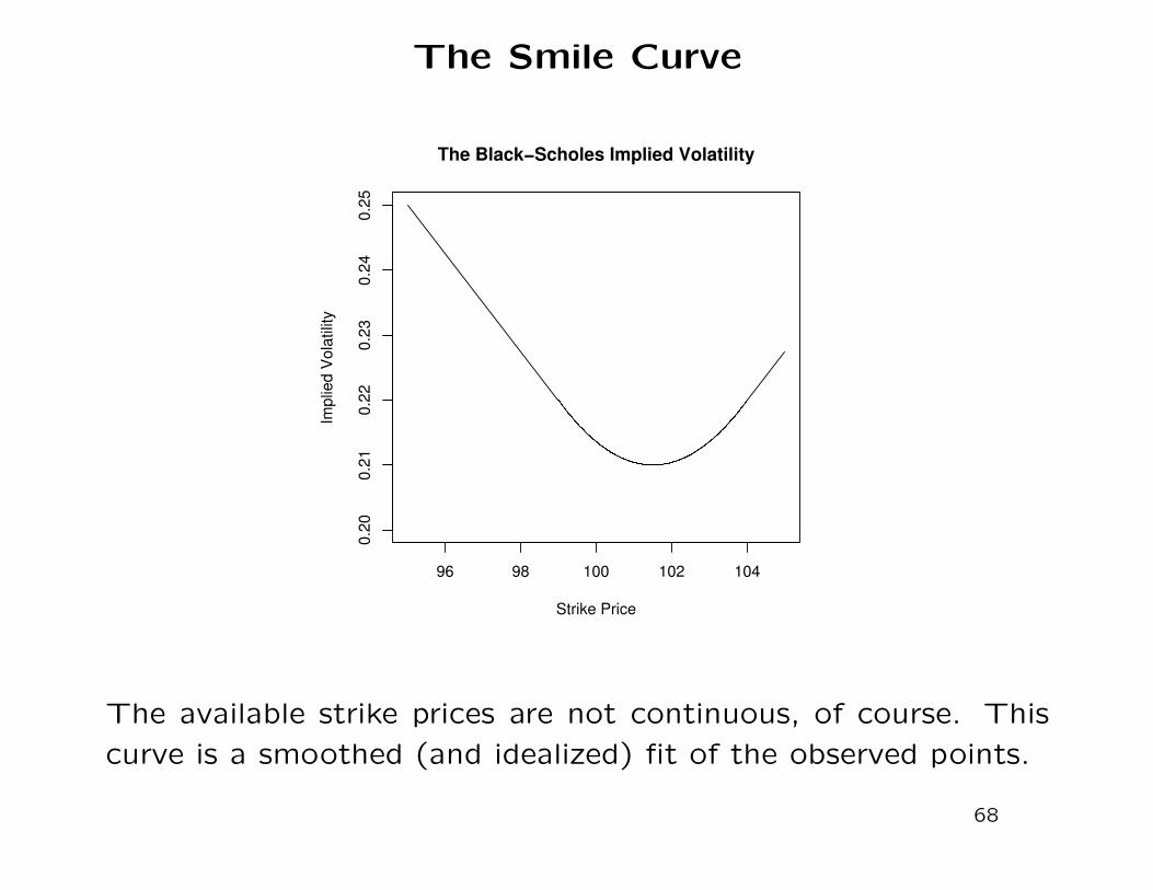
The Smile Curve

96 98 100 102 104

0.2

00.2

10.2

20.2

30.2

40.2

5

Strike Price

Implie

d V

ola

tilit

y

The Black−Scholes Implied Volatility

The available strike prices are not continuous, of course. This

curve is a smoothed (and idealized) fit of the observed points.

68

The Smile Curve

The smile curve is not well-understood, although we have a lot

of empirical observations on it.

Interestingly, prior to the 1987 crash, the minimum of the smile

curve was at or near the market price St.

Since then it is generally at a point larger than the market price.

69

Computations of Black-Scholes Implied

Volatility

The Black-Scholes price depends on being able to evaluate the

standard normal CDF, and the implied volatility depends on being

able to evaluate the standard normal PDF.

The PDF is easy to compute from the definition: f(x) = e−x2/2/√

2π.

The CDF is more difficult.

In R, the CDF is computed by pnorm and the PDF by dnorm.

In Statistics Toolbox of Matlab, the CDF is computed by normcdf

and the PDF by normpdf.

Without the Statistics Toolbox, in Matlab, the CDF can be com-

puted at the point x by (1 + (erf(x/sqrt(2))))./2.

70

Variation in Volatility over Time

The volatility also varies in time. There are periods of high

volatility and other periods of low volatility. This is called “volatil-

ity clustering”.

The volatility of an index is somewhat similar to that of an

individual stock. The volatility of an index is a reflection of

market sentiment. (There are various ways of interpreting this!)

In general, a declining market is viewed as “more risky” than a

rising market, and hence, it is generally true that the volatility

in a declining market is higher.

Contrarians believe high volatility is bullish because it lags market

trends.

71

Measuring the Volatility of the Market

A standard measure of the overall volatility of the market is the

CBOE Volatility Index, VIX, which CBOE introduced in 1993 as

a weighted average of the Black-Scholes-implied volatilities of

the S&P 100 Index from at-the-money near-term call and put

options.

(“At-the-money” is defined as the strike price with the smallest

difference between the call price and the put price.)

In 2004, futures on the VIX began trading on the CBOE Futures

Exchange (CFE), and in 2006, CBOE listed European-style calls

and puts on the VIX.

Another measure is the CBOE Nasdaq Volatility Index, VXN,

which CBOE computes from the Nasdaq-100 Index, NDX, sim-

ilarly to the VIX. (Note that the more widely-watched Nasdaq

Index is the Composite, IXIC.)

72

The VIX

In 2006, CBOE changed the way the VIX is computed. It is

now based on the volatilities of the S&P 500 Index implied by

several call and put options, not just those at the money, and it

uses near-term and next-term options (where “near-term” is the

earliest expiry mover than 8 days away).

It is no longer computed from the Black-Scholes formula.

It uses the prices of calls with strikes above the current price of

the underlying, starting with the first out-of-the money call and

sequentially including all with higher strikes until two consecutive

such calls have no bids. It uses the prices of puts with strikes

below the current price of the underlying in a similar manner.

The price of an option is the “mid-quote” price, i.e. the average

of the bid and ask prices.

73

Technical Details: Computing the VIX

Let K1 = K2 < K3 < · · · < Kn−1 < Kn = Kn+1 be the strikeprices of the options that are to be used.

The VIX is defined as 100 × σ, where

σ2 = 2erT

T

(

∑ni=2;i 6=j

∆KiK2

iQ(Ki) +

∆Kj

K2j

(

Q(Kjput) + Q(Kjcall))

/2

)

−1T

(

FKj

− 1

)2,

•T is the time to expiry (in our usual notation, we would useT − t, but we can let t = 0),•F , called the “forward index level”, is the at-the-money strikeplus erT times the difference in the call and put prices for thatstrike,•Ki is the strike price of the ith out-of-the-money strike price(that is, of a put if Ki < F and of a call if F < Ki),•∆Ki = (Ki+1 − Ki−1)/2,•Q(Ki) is the mid-quote price of the option,•r is the risk-free interest rate, and•Kj is the largest strike price less than F .

74

Technical Details: Computing the VIX

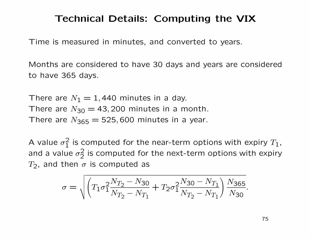
Time is measured in minutes, and converted to years.

Months are considered to have 30 days and years are considered

to have 365 days.

There are N1 = 1,440 minutes in a day.

There are N30 = 43,200 minutes in a month.

There are N365 = 525,600 minutes in a year.

A value σ21 is computed for the near-term options with expiry T1,

and a value σ22 is computed for the next-term options with expiry

T2, and then σ is computed as

σ =

√

√

√

√

(

T1σ21

NT2− N30

NT2− NT1

+ T2σ21

N30 − NT1

NT2− NT1

)

N365

N30.

75