GeneralizedLinearModels - ut · Tweediedistributionwith1
22
Generalized Linear Models Lecture 12. Tweedie models. Compound Poisson models GLM (Spring, 2018) Lecture 12 1 / 22
Transcript of GeneralizedLinearModels - ut · Tweediedistributionwith1
Generalized Linear ModelsLecture 12. Tweedie models. Compound Poisson models
GLM (Spring, 2018) Lecture 12 1 / 22
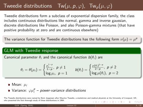
Tweedie distributions Tw(µ, p, ϕ), Twp(µ, ϕ)Tweedie distributions form a subclass of exponential dispersion family, the classincludes continuous distributions like normal, gamma and inverse gaussian,discrete distributions like Poisson, and also Poisson-gamma mixtures (that havepositive probability at zero and are continuous elsewhere)
The variance function for Tweedie distributions has the following form ν(µ) = µp
GLM with Tweedie responseCanonical parameter θi and the canonical function b(θi ) are
θi = θ(µi ) ={µ1−p
i1−p , p 6= 1logµi , p = 1
b(θi ) ={µ(θi )2−p
2−p , p 6= 2logµ(θi ), p = 2
Mean: µi
Variance: ϕµpi – power-variance distributions
The Tweedie distributions were named by Bent Jorgensen after Maurice Tweedie, a statistician and medical physicist at the University of Liverpool, UK,who presented the first thorough study of these distributions in 1984.
GLM (Spring, 2018) Lecture 12 2 / 22
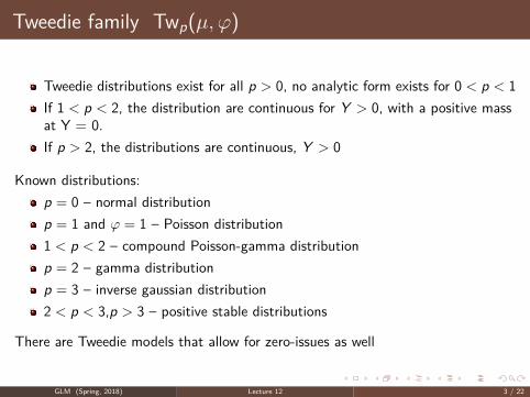
Tweedie family Twp(µ, ϕ)
Tweedie distributions exist for all p > 0, no analytic form exists for 0 < p < 1If 1 < p < 2, the distribution are continuous for Y > 0, with a positive massat Y = 0.If p > 2, the distributions are continuous, Y > 0
Known distributions:p = 0 – normal distributionp = 1 and ϕ = 1 – Poisson distribution1 < p < 2 – compound Poisson-gamma distributionp = 2 – gamma distributionp = 3 – inverse gaussian distribution2 < p < 3,p > 3 – positive stable distributions
There are Tweedie models that allow for zero-issues as well
GLM (Spring, 2018) Lecture 12 3 / 22
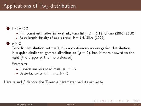
Applications of Twp distribution
1 1 < p < 2Fish count estimation (silky shark, tuna fish): p̂ = 1.12, Shono (2008, 2010)Root length density of apple trees: p̂ = 1.4, Silva (1999)
2 p ≥ 2Tweedie distribution with p ≥ 2 is a continuous non-negative distribution.It is quite similar to gamma distribution (p = 2), but is more skewed to theright (the bigger p, the more skewed)Examples:
Survival analysis of animals: p̂ = 3.85Butterfat content in milk: p̂ ≈ 5
Here p and p̂ denote the Tweedie parameter and its estimate
GLM (Spring, 2018) Lecture 12 4 / 22
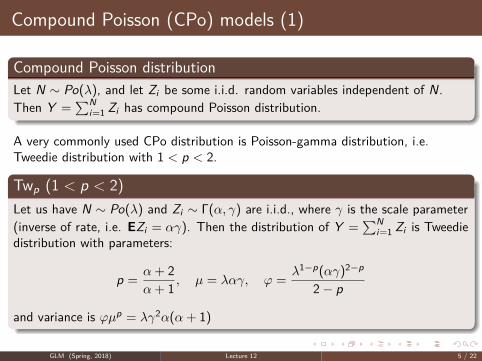
Compound Poisson (CPo) models (1)
Compound Poisson distributionLet N ∼ Po(λ), and let Zi be some i.i.d. random variables independent of N.Then Y =
∑Ni=1 Zi has compound Poisson distribution.
A very commonly used CPo distribution is Poisson-gamma distribution, i.e.Tweedie distribution with 1 < p < 2.
Twp (1 < p < 2)Let us have N ∼ Po(λ) and Zi ∼ Γ(α, γ) are i.i.d., where γ is the scale parameter(inverse of rate, i.e. EZi = αγ). Then the distribution of Y =
∑Ni=1 Zi is Tweedie
distribution with parameters:
p = α + 2α + 1 , µ = λαγ, ϕ = λ1−p(αγ)2−p
2− p
and variance is ϕµp = λγ2α(α + 1)
GLM (Spring, 2018) Lecture 12 5 / 22
Compound Poisson (CPo) models (2)
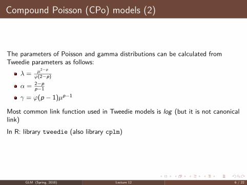
The parameters of Poisson and gamma distributions can be calculated fromTweedie parameters as follows:
λ = µ2−p
ϕ(2−p)
α = 2−pp−1
γ = ϕ(p − 1)µp−1
Most common link function used in Tweedie models is log (but it is not canonicallink)
In R: library tweedie (also library cplm)
GLM (Spring, 2018) Lecture 12 6 / 22
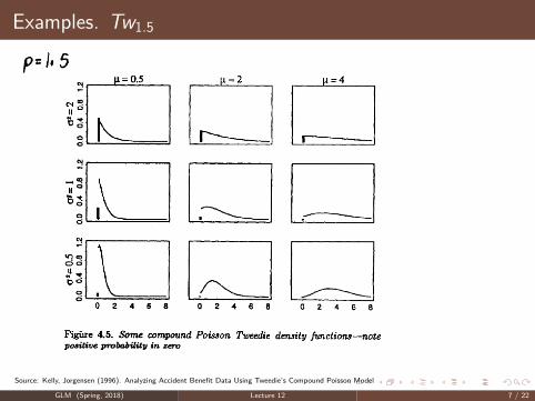
Examples. Tw1.5
Source: Kelly, Jorgensen (1996). Analyzing Accident Benefit Data Using Tweedie’s Compound Poisson Model
GLM (Spring, 2018) Lecture 12 7 / 22
Example. Non-life insurance claim payments (1)
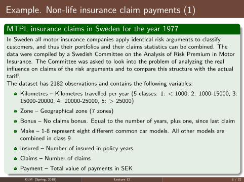
MTPL insurance claims in Sweden for the year 1977In Sweden all motor insurance companies apply identical risk arguments to classifycustomers, and thus their portfolios and their claims statistics can be combined. Thedata were compiled by a Swedish Committee on the Analysis of Risk Premium in MotorInsurance. The Committee was asked to look into the problem of analyzing the realinfluence on claims of the risk arguments and to compare this structure with the actualtariff.The dataset has 2182 observations and contains the following variables:
Kilometres – Kilometres travelled per year (5 classes: 1: < 1000, 2: 1000-15000, 3:15000-20000, 4: 20000-25000, 5: > 25000)Zone – Geographical zone (7 zones)Bonus – No claims bonus. Equal to the number of years, plus one, since last claimMake – 1-8 represent eight different common car models. All other models arecombined in class 9Insured – Number of insured in policy-yearsClaims – Number of claimsPayment – Total value of payments in SEK
GLM (Spring, 2018) Lecture 12 8 / 22
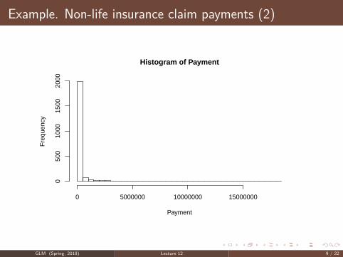
Example. Non-life insurance claim payments (2)
Histogram of Payment
Payment
Fre
quen
cy
0 5000000 10000000 15000000
050
010
0015
0020
00
GLM (Spring, 2018) Lecture 12 9 / 22
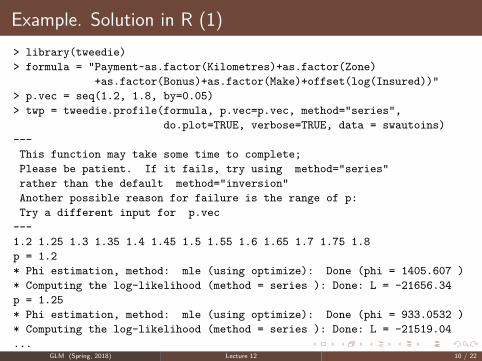
Example. Solution in R (1)> library(tweedie)> formula = "Payment~as.factor(Kilometres)+as.factor(Zone)
+as.factor(Bonus)+as.factor(Make)+offset(log(Insured))"> p.vec = seq(1.2, 1.8, by=0.05)> twp = tweedie.profile(formula, p.vec=p.vec, method="series",
do.plot=TRUE, verbose=TRUE, data = swautoins)---This function may take some time to complete;Please be patient. If it fails, try using method="series"rather than the default method="inversion"Another possible reason for failure is the range of p:Try a different input for p.vec
---1.2 1.25 1.3 1.35 1.4 1.45 1.5 1.55 1.6 1.65 1.7 1.75 1.8p = 1.2* Phi estimation, method: mle (using optimize): Done (phi = 1405.607 )* Computing the log-likelihood (method = series ): Done: L = -21656.34p = 1.25* Phi estimation, method: mle (using optimize): Done (phi = 933.0532 )* Computing the log-likelihood (method = series ): Done: L = -21519.04...
GLM (Spring, 2018) Lecture 12 10 / 22
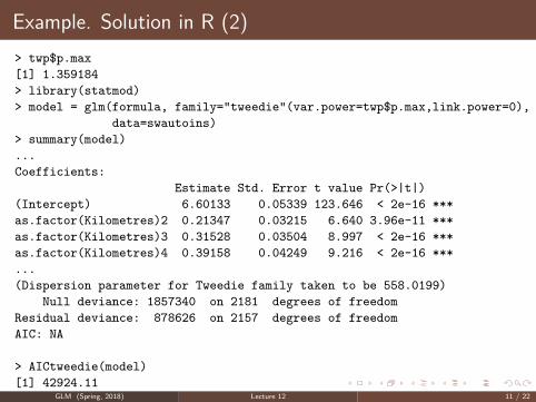
Example. Solution in R (2)> twp$p.max[1] 1.359184> library(statmod)> model = glm(formula, family="tweedie"(var.power=twp$p.max,link.power=0),
data=swautoins)> summary(model)...Coefficients:
Estimate Std. Error t value Pr(>|t|)(Intercept) 6.60133 0.05339 123.646 < 2e-16 ***as.factor(Kilometres)2 0.21347 0.03215 6.640 3.96e-11 ***as.factor(Kilometres)3 0.31528 0.03504 8.997 < 2e-16 ***as.factor(Kilometres)4 0.39158 0.04249 9.216 < 2e-16 ***...(Dispersion parameter for Tweedie family taken to be 558.0199)
Null deviance: 1857340 on 2181 degrees of freedomResidual deviance: 878626 on 2157 degrees of freedomAIC: NA
> AICtweedie(model)[1] 42924.11
GLM (Spring, 2018) Lecture 12 11 / 22
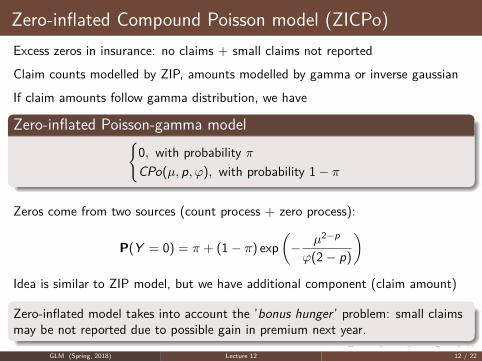
Zero-inflated Compound Poisson model (ZICPo)Excess zeros in insurance: no claims + small claims not reported
Claim counts modelled by ZIP, amounts modelled by gamma or inverse gaussian
If claim amounts follow gamma distribution, we have
Zero-inflated Poisson-gamma model{0, with probability πCPo(µ, p, ϕ), with probability 1− π
Zeros come from two sources (count process + zero process):
P(Y = 0) = π + (1− π) exp(− µ2−p
ϕ(2− p)
)Idea is similar to ZIP model, but we have additional component (claim amount)
Zero-inflated model takes into account the ’bonus hunger ’ problem: small claimsmay be not reported due to possible gain in premium next year.
GLM (Spring, 2018) Lecture 12 12 / 22
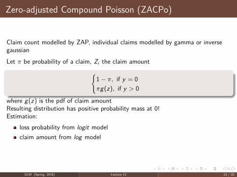
Zero-adjusted Compound Poisson (ZACPo)
Claim count modelled by ZAP, individual claims modelled by gamma or inversegaussian
Let π be probability of a claim, Zi the claim amount{1− π, if y = 0πg(z), if y > 0
where g(z) is the pdf of claim amountResulting distribution has positive probability mass at 0!Estimation:
loss probability from logit modelclaim amount from log model
GLM (Spring, 2018) Lecture 12 13 / 22
Example. Australian insurance claims 2004-2005
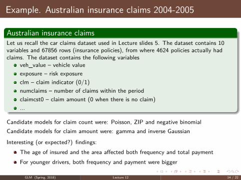
Australian insurance claimsLet us recall the car claims dataset used in Lecture slides 5. The dataset contains 10variables and 67856 rows (insurance policies), from where 4624 policies actually hadclaims. The dataset contains the following variables
veh_value – vehicle valueexposure – risk exposureclm – claim indicator (0/1)numclaims – number of claims within the periodclaimcst0 – claim amount (0 when there is no claim)...
Candidate models for claim count were: Poisson, ZIP and negative binomialCandidate models for claim amount were: gamma and inverse Gaussian
Interesting (or expected?) findings:The age of insured and the area affected both frequency and total paymentFor younger drivers, both frequency and payment were bigger
GLM (Spring, 2018) Lecture 12 14 / 22
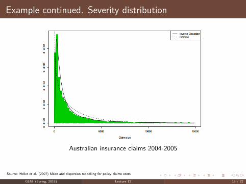
Example continued. Severity distribution
Australian insurance claims 2004-2005
Source: Heller et al. (2007) Mean and dispersion modelling for policy claims costs
GLM (Spring, 2018) Lecture 12 15 / 22
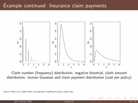
Example continued. Insurance claim payments
Claim number (frequency) distribution: negative binomial, claim amountdistribution: inverse Gaussian and claim payment distribution (cost per policy)
Source: Heller et al. (2007) Mean and dispersion modelling for policy claims costs
GLM (Spring, 2018) Lecture 12 16 / 22
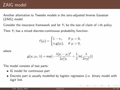
ZAIG model
Another alternative to Tweedie models is the zero-adjusted Inverse Gaussian(ZAIG) model
Consider the insurance framework and let Yi be the size of claim of i-th policy
Then Yi has a mixed discrete-continuous probability function:
f (yi ) ={1− πi , if yi = 0,πig(yi ), if yi > 0,
whereg(yi ;µi , λ) = exp{−λ(yi − µi )2
2µ2i yi+ 1
2 ln( λ
2πy3i
)}
The model consists of two parts:IG model for continuous partDiscrete part is usually modelled by logistic regression (i.e. binary model withlogit link
GLM (Spring, 2018) Lecture 12 17 / 22
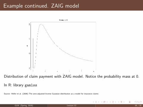
Example continued. ZAIG model
Distribution of claim payment with ZAIG model. Notice the probability mass at 0.
In R: library gamlss
Source: Heller et al. (2006) The zero-adjusted Inverse Gaussian distribution as a model for insurance claims
GLM (Spring, 2018) Lecture 12 18 / 22
Applications of CPo distribution in climatology
Different applications of Tweedie model to weather data:Analysis of rainy days in Melbourne (1981-1990), p̂ = 1.58Analysis of snowfall data in Seattle (1906–1960), p̂ = 1.52Average wind speed in Ireland (1961–1978), 1 < p̂ < 2
Here p̂ is the estimated Tweedie index
Modelling rainfall data (Dunn et al, 1996, Lennox, 2003)Model:
Dry days (rainfall amount is 0) and rainy days (rainfall amount > 0, treatedas continuous r.v.)Rainfall amount follows gamma distributionRainy days follow Poisson distribution
GLM (Spring, 2018) Lecture 12 19 / 22
Applications of CPo in sociology and medicine
Alcohol use among British teenagers (Gilchrist, Drinkwater (1999)Cohort study among 16-17 year old teenagers, n = 1545Model:
number of events of consumption is Poisson distributedthe amount drunk on each occasion is gamma distributedtotal amount is Tweedie distributed (p̂ = 1.41)
Time-Use Data, TUD-data (Dunn&Brown, 2011)Longitudinal study of Australian children (march-nov 2004), 4-5 y.o. children, 3456diaries with dataAnalysis of time spent on different activities was conducted, data contains many zeros,the non-zero part is treated as continuous
3 response variables: time spent on watching TV, traveling and walkingArguments used: weekday, sex, number of children, income of family, education ofparents, etc
GLM (Spring, 2018) Lecture 12 20 / 22
Example. Time-use dataIn average, 4-5 year old children spent
more than 2 hours a day watching TVless than 1 hour traveling by carless than 15 minutes walking
Corresponding medians:TV: 1.8 hourscar: 0.8 hourswalking: 0 hours
Results of Tweedie model:Tweedie indices: tv: p̂ = 1.18, car: p̂ = 1.19, walking: p̂ = 1.32weekday, income, mother’s job – significant for tv-use, not for othersfather’s job not significant for walkingchild’s sex not significant for travelingnumber of children significant for traveling
Tweedie model is compared by tobit model and linear model and considered betterSource: Brown, J.E., Dunn, P.K. (2011). Comparisons of Tobit, Linear, and Poisson-Gamma Regression Models. An Application of Time Use Data.Sociological Methods and Research, 40(3), 511–535
GLM (Spring, 2018) Lecture 12 21 / 22
Summary. Compound Poisson models
Compound Poisson models:Compound Poisson distribution as a special case of Tweedie distribution(1 < p < 2), Poisson + Gamma
General compound Poisson distribution (CPo): Poisson + (usuallycontinuous) distribution
ZICPo – zero-inflated compound Poisson distribution (in case of excess zeros)
ZACPo – zero-altered compound Poisson distribution (in case of excess zeros,when zeros itself are not of interest)
GLM (Spring, 2018) Lecture 12 22 / 22

![p pacemaker ό ɔ padde ɔ ά Χɔ padder Χɔ padde- Χɔ padle ɔ ... · : pakk deg godt inn før du går ut ί ά έ [tiliks ɔ kala prin vjis ks ɔ ] / pakke ut/opp ά [ks pak](https://static.fdocument.org/doc/165x107/5e0f9f236c4ebd44711e5b28/p-pacemaker-oe-padde-padder-padde-padle-pakk-deg.jpg)