Generalized eigenvectorpmh/teach/algebra/additional/eigen.pdf · 2013-03-18 · that this matrix is...

Generalized eigenvectorFrom Wikipedia, the free encyclopedia

In linear algebra, for a matrix A, there may not always exist a full set of linearly independent eigenvectorsthat form a complete basis – a matrix may not be diagonalizable. This happens when the algebraicmultiplicity of at least one eigenvalue λ is greater than its geometric multiplicity (the nullity of the matrix

, or the dimension of its nullspace). In such cases, a generalized eigenvector of A is a nonzerovector v, which is associated with λ having algebraic multiplicity k ≥1, satisfying

The set of all generalized eigenvectors for a given λ, together with the zero vector, form the generalizedeigenspace for λ.

Ordinary eigenvectors and eigenspaces are obtained for k=1.

Contents

1 For defective matrices2 Examples

2.1 Example 12.2 Example 2

3 Other meanings of the term4 The Nullity of (A − λ I)k

4.1 Introduction4.2 Existence of Eigenvalues4.3 Constructive proof of Schur's triangular form4.4 Nullity Theorem's Proof

5 Motivation of the Procedure5.1 Introduction5.2 Notation5.3 Preliminary Observations5.4 Recursive Procedure5.5 Generalized Eigenspace Decomposition5.6 Powers of a Matrix

5.6.1 using generalized eigenvectors5.6.2 the minimal polynomial of a matrix5.6.3 using confluent Vandermonde matrices5.6.4 using difference equations

5.7 Chains of generalized eigenvectors5.7.1 Differential equations y′= Ay5.7.2 Revisiting the powers of a matrix

5.8 Ordinary linear difference equations6 References

For defective matrices

Generalized eigenvectors are needed to form a complete basis of a defective matrix, which is a matrix inwhich there are fewer linearly independent eigenvectors than eigenvalues (counting multiplicity). Over an

Generalized eigenvector - Wikipedia, the free encyclopedia http://en.wikipedia.org/wiki/Generalized_eigenvector

1 of 30 18/03/2013 20:00

algebraically closed field, the generalized eigenvectors do allow choosing a complete basis, as follows fromthe Jordan form of a matrix.

In particular, suppose that an eigenvalue λ of a matrix A has an algebraic multiplicity m but fewercorresponding eigenvectors. We form a sequence of m eigenvectors and generalized eigenvectors

that are linearly independent and satisfy

for some coefficients , for . It follows that

The vectors can always be chosen, but are not uniquely determined by the aboverelations. If the geometric multiplicity (dimension of the eigenspace) of λ is p, one can choose the first pvectors to be eigenvectors, but the remaining m − p vectors are only generalized eigenvectors.

Examples

Example 1

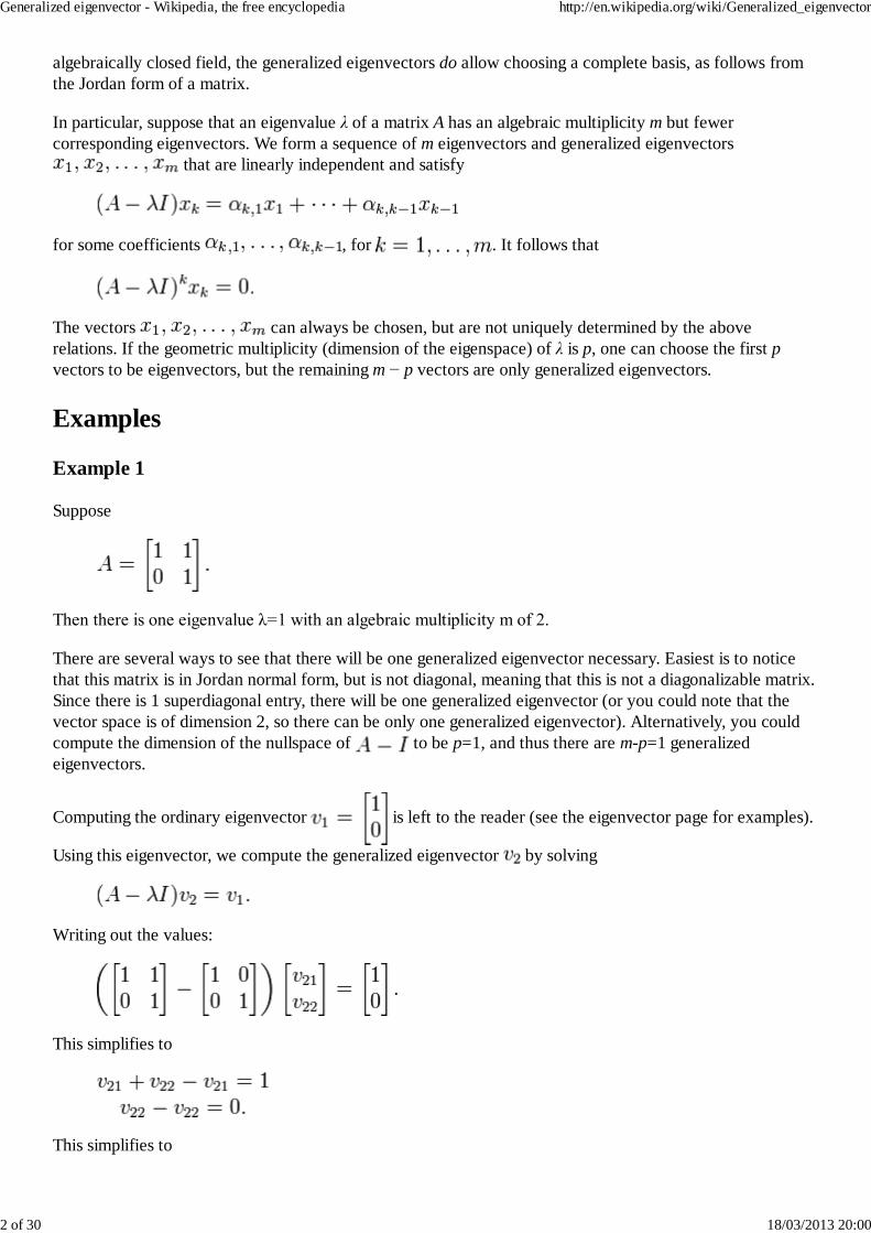
Suppose

Then there is one eigenvalue λ=1 with an algebraic multiplicity m of 2.

There are several ways to see that there will be one generalized eigenvector necessary. Easiest is to noticethat this matrix is in Jordan normal form, but is not diagonal, meaning that this is not a diagonalizable matrix.Since there is 1 superdiagonal entry, there will be one generalized eigenvector (or you could note that thevector space is of dimension 2, so there can be only one generalized eigenvector). Alternatively, you couldcompute the dimension of the nullspace of to be p=1, and thus there are m-p=1 generalizedeigenvectors.

Computing the ordinary eigenvector is left to the reader (see the eigenvector page for examples).

Using this eigenvector, we compute the generalized eigenvector by solving

Writing out the values:

This simplifies to

This simplifies to


2 of 30 18/03/2013 20:00

And has no restrictions and thus can be any scalar. So the generalized eigenvector is , where

the * indicates that any value is fine. Usually picking 0 is easiest.

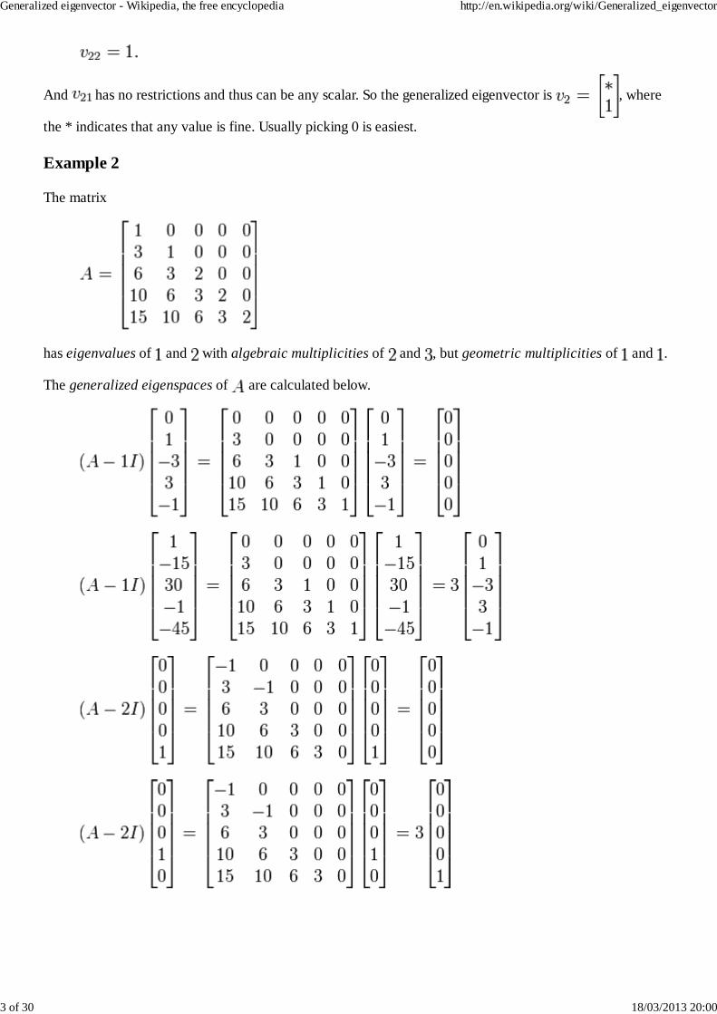
Example 2

The matrix

has eigenvalues of and with algebraic multiplicities of and , but geometric multiplicities of and .

The generalized eigenspaces of are calculated below.


3 of 30 18/03/2013 20:00

This results in a basis for each of the generalized eigenspaces of . Together they span the space of all 5dimensional column vectors.

The Jordan Canonical Form is obtained.

where

Other meanings of the term

The usage of generalized eigenfunction differs from this; it is part of the theory of rigged Hilbertspaces, so that for a linear operator on a function space this may be something different.

One can also use the term generalized eigenvector for an eigenvector of the generalized eigenvalueproblem

The Nullity of (A − λ I)k

Introduction

In this section it is shown, when is an eigenvalue of a matrix with algebraic multiplicity , then thenull space of has dimension .

Existence of Eigenvalues

Consider a nxn matrix A. The determinant of A has the fundamental properties of beingn linear and alternating. Additionally det(I) = 1, for I the nxn identity matrix. From thedeterminant's definition it can be seen that for a triangular matrix T = (tij) that


4 of 30 18/03/2013 20:00

det(T) = ∏(tii).

There are three elementary row operations, scalar multiplication, interchange of two rows,and the addition of a scalar multiple of one row to another. Multiplication of a row of A by αresults in a new matrix whose determinant is α det(A). Interchange of two rows changes thesign of the determinant, and the addition of a scalar multiple of one row to another does notaffect the determinant.

The following simple theorem holds, but requires a little proof.

Theorem:The equation A x = 0 has a solution x ≠ 0, if and only if det(A) = 0.

proof:Given the equation A x = 0 attempt to solve it using the elementary row operationsof addition of a scalar multiple of one row to another and row interchanges only,until an equivalent equation U x = 0 has been reached, with U an upper triangular matrix.Since det(U) = ±det(A) and det(U) = ∏(uii)we have that det(A) = 0 if and only if at least one uii = 0. The back substitution procedureas performed after Gaussian Elimination will allow placing at least one non zero elementin x when there is a uii = 0. When all uii ≠ 0 back substitution will require x = 0.

Theorem:The equation A x = λ x has a solution x ≠ 0, if and only if det( λ I − A) = 0.

proof:The equation A x = λ x is equivalent to ( λ I − A) x = 0.

Constructive proof of Schur's triangular form

The proof of the main result of this section will rely on the similarity transformation as stated and provennext.

Theorem: Schur Transformation to Triangular Form Theorem

For any n×n matrix A, there exists a triangular matrix T and a unitary matrix Q, such that A Q = Q T. (The transformations are not unique, but are related.)

Proof:

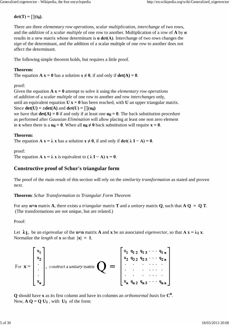
Let λ1, be an eigenvalue of the n×n matrix A and x be an associated eigenvector, so that A x = λ1 x.Normalize the length of x so that |x| = 1.

Q should have x as its first column and have its columns an orthonormal basis for Cn.Now, A Q = Q U1 , with U1 of the form:


5 of 30 18/03/2013 20:00

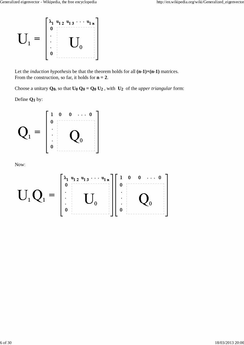
Let the induction hypothesis be that the theorem holds for all (n-1)×(n-1) matrices.From the construction, so far, it holds for n = 2.

Choose a unitary Q0, so that U0 Q0 = Q0 U2 , with U2 of the upper triangular form:

Define Q1 by:

Now:


6 of 30 18/03/2013 20:00

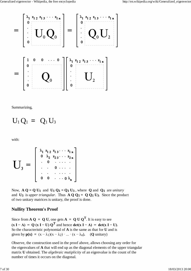
Summarizing,

U1

Q1

=

Q1

U3

with:

Now, A Q = Q U1 and U1 Q1 = Q1 U3 , where Q and Q1 are unitaryand U3 is upper triangular. Thus A Q Q1 = Q Q1 U3. Since the productof two unitary matrices is unitary, the proof is done.

Nullity Theorem's Proof

Since from A Q = Q U, one gets A = Q U QT. It is easy to see(x I − A) = Q (x I − U) QT and hence det(x I − A) = det(x I − U).So the characteristic polynomial of A is the same as that for U and isgiven by p(x) = (x − λ1)(x − λ2) · ... · (x − λn). (Q unitary)

Observe, the construction used in the proof above, allows choosing any order forthe eigenvalues of A that will end up as the diagonal elements of the upper triangularmatrix U obtained. The algebraic mutiplicity of an eigenvalue is the count of thenumber of times it occurs on the diagonal.


7 of 30 18/03/2013 20:00

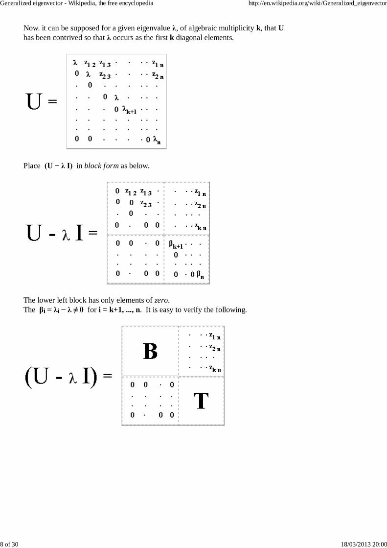
Now. it can be supposed for a given eigenvalue λ, of algebraic multiplicity k, that Uhas been contrived so that λ occurs as the first k diagonal elements.

Place (U − λ I) in block form as below.

The lower left block has only elements of zero.The βi = λi − λ ≠ 0 for i = k+1, ..., n. It is easy to verify the following.


8 of 30 18/03/2013 20:00

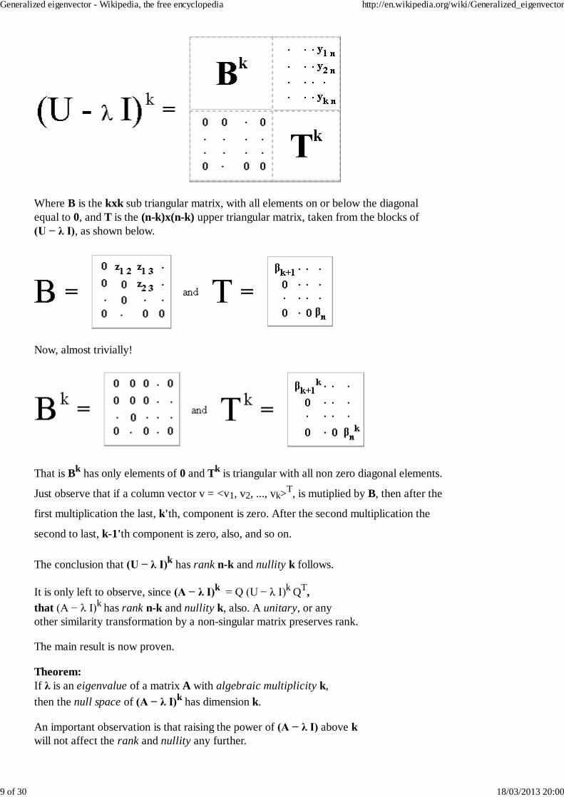
Where B is the kxk sub triangular matrix, with all elements on or below the diagonalequal to 0, and T is the (n-k)x(n-k) upper triangular matrix, taken from the blocks of(U − λ I), as shown below.

Now, almost trivially!

That is Bk has only elements of 0 and Tk is triangular with all non zero diagonal elements.

Just observe that if a column vector v = <v1, v2, ..., vk>T, is mutiplied by B, then after the

first multiplication the last, k'th, component is zero. After the second multiplication the

second to last, k-1'th component is zero, also, and so on.

The conclusion that (U − λ I)k has rank n-k and nullity k follows.

It is only left to observe, since (A − λ I)k = Q (U − λ I)k QT,that (A − λ I)k has rank n-k and nullity k, also. A unitary, or anyother similarity transformation by a non-singular matrix preserves rank.

The main result is now proven.

Theorem:If λ is an eigenvalue of a matrix A with algebraic multiplicity k,then the null space of (A − λ I)k has dimension k.

An important observation is that raising the power of (A − λ I) above kwill not affect the rank and nullity any further.


9 of 30 18/03/2013 20:00

Motivation of the Procedure

Introduction

In the section Existence of Eigenvalues it was shown that whena nxn matrix A, has an eigenvalue λ, of algebraic multiplicity k,then the null space of (A − λ I)k, has dimension k.

The Generalized Eigenspace of A, λ will be defined to be the null spaceof (A − λ I)k. Many authors prefer to call this the kernel of (A − λ I)k.

Notice that if a nxn matrix has eigenvalues λ1, λ2, ..., λr withalgebraic multiplicities k1, k2, ..., kr, then k1 + k2 + ... + kr = n.

It will turn out that any two generalized eigenspaces of A, associated withdifferent eigenvalues, will have a trivial intersection of {0}. From this itfollows that the generalized eigenspaces of A combined span Cn,the set of all n dimensional column vectors of complex numbers.

The motivation for using a recursive procedure starting with theeigenvectors of A and solving for a basis of the generalized eigenspaceof A, λ using the matix (A − λ I), will be expounded on.

Notation

Some notation is introduced to help abbreviate statements.

Cn is the vector space of all n dimensional column vectors of complex numbers.The Null Space of A, N(A) = {x: A x = 0}.V ⊆ W will mean V is a subset of W.V ⊂ W will mean V is a proper subset of W.A(V) = {y: y = A x, for some x ∈ V}.W \ V will mean { x: x ∈ W and x is not in V}.The Range of A is A(Cn) and will be denoted by R(A).dim(V) will stand for the dimension of V.{0} will stand for the trivial subspace of Cn.

Preliminary Observations

Throughout this discussion it is assumed that A is a nxn matrix of complex numbers.

Since Am x = A (Am-1 x), the inclusions

N(A) ⊆ N(A2) ⊆ ... ⊆ N(Am-1) ⊆ N(Am),

are obvious. Since Am x = Am-1(A x), the inclusions

R(A) ⊇ R(A2) ⊇ ... ⊇ R(Am-1) ⊇ R(Am),

are clear too.


10 of 30 18/03/2013 20:00

Theorem:When the more trivial case N(A2) = N(A), does not hold,there exists k ≥ 2, such that the inclusions,N(A) ⊂ N(A2) ⊂ ... ⊂ N(Ak-1) ⊂ N(Ak) = N(Ak+1) = ...,andR(A) ⊃ R(A2) ⊃ ... ⊃ R(Ak-1) ⊃ R(Ak) = R(Ak+1) = ...,are proper.

proof:

0 ≤ dim(R(Am+1)) ≤ dim(R(Am)) so eventually dim(R(Am+1)) = dim(R(Am)),for some m. From the inclusion R(Am+1) ⊆ R(Am) it is seen that a basis forR(Am+1) is a basis for R(Am) too. That is R(Am+1) = R(Am).Since R(Am+1) = A(R(Am)), when R(Am+1) = R(Am), it will beR(Am+2) = A(R(Am+1)) = A(R(Am)) = R(Am+1).By the rank nullity theorem, it will also be the case thatdim(N(Am+2)) = dim(N(Am+1)) = dim(N(Am)), for the same m.From the inclusions N(Am+2) ⊆ N(Am+1) ⊆ N(Am),it is clear that a basis for N(Am+2) is also a basis for N(Am+1) and N(Am).So N(Am+2) = N(Am+1) = N(Am).Now, k is the first m for which this happens.

Since certain expressions will occur many times in the following,some more notation will be introduced.

Aλ, k = (A − λ I)k

Nλ, k = N((A − λ I)k) = N(Aλ, k)Rλ, k = R((A − λ I)k) = R(Aλ, k)

From the inclusions Nλ, 1 ⊂ Nλ, 2 ⊂ ... ⊂ Nλ, k-1 ⊂ Nλ, k = Nλ, k+1 = ..., Nλ, k \ {0} = ∪ (Nλ, m \ Nλ, m-1), for m = 1, ..., k and Nλ, 0 = {0}, follows.

When λ is an eigenvalue of A, in the statement above, k will not exceed thealgebraic multiplicity of λ, and can be less. In fact when k would only be 1 iswhen there is a full set of linearly independent eigenvectors. Let's consider when k ≥ 2 .

Now, x ∈ Nλ, m \ Nλ, m-1, if and only if Aλ, m x = 0, and Aλ, m-1 x ≠ 0 . Make the observationthat Aλ, m x = 0, and Aλ, m-1 x ≠ 0 ,if and only if Aλ, m-1 Aλ, 1 x = 0, and Aλ, m-2 Aλ, 1 x ≠ 0 .

So, x ∈ Nλ, m \ Nλ, m-1, if and only if Aλ, 1 x ∈ Nλ, m-1 \ Nλ, m-2.

Recursive Procedure

Consider a matrix A, with an eigenvalue λ of algebraic multiplicity k ≥ 2,such that there are not k linearly independent eigenvectors associated with λ.

It is desired to extend the eigenvectors to a basis for Nλ, k. That is a basis forthe generalized eigenvectors associated with λ.


11 of 30 18/03/2013 20:00

There exists some 2 ≤ r ≤ k , such that

Nλ, 1 ⊂ Nλ, 2 ⊂ ... ⊂ Nλ, r-1 ⊂ Nλ, r = Nλ, r+1 = ..., Nλ, r \ {0} = ∪ (Nλ, m \ Nλ, m-1), for m = 1, ..., r and Nλ, 0 = {0}, .

The eigenvectors are Nλ, 1 \ {0}, so let x1, ..., xr1 be a basis for Nλ, 1 \ {0}.

Note that each Nλ, m is a subspace and so a basis for Nλ, m-1can be extended to a basis for Nλ, m .

Because of this we can expect to find some r2 = dim(Nλ, 2) − dim(Nλ, 1)

linearly independent vectors

xr1+ 1, ..., xr1+ r2 such that x1, ..., xr1 , xr1+ 1, ..., xr1+ r2

is a basis for Nλ, 2

Now, x ∈ Nλ, 2 \ Nλ, 1, if and only if Aλ, 1 x ∈ Nλ, 1 \ {0}.

Thus we can expect that for each x ∈ {xr1+ 1, ..., xr1+ r2} ,Aλ, 1 x = α1 x1 + ... + αr1 xr1 ,for some α1, ..., αr1 , depending on x.

Suppose we have reached the stage in the construction so that m-1 sets,

{x1, ..., xr1} , {xr1+ 1, ..., xr1+ r2} , ..., {xr1+ ... + rm-2+ 1, ..., xr1+ ... + rm-1}

such that

x1, ..., xr1 , xr1+ 1, ..., xr1+ r2 , ..., xr1+ ... + rm-2 + 1, ..., xr1+ ... + rm-1

is a basis for Nλ, m-1 , have been found.

We can expect to find some rm = dim(Nλ, m) − dim(Nλ, m-1)

linearly independent vectors

xr1+ ... + rm-1+ 1, ..., xr1+ ... + rm such that

x1, ..., xr1 , xr1+ 1, ..., xr1+ r2 , ..., xr1+ ... + rm-1 + 1, ..., xr1+ ... + rm

is a basis for Nλ, m

Again, x ∈ Nλ, m \ Nλ, m-1, if and only if Aλ, 1 x ∈ Nλ, m-1 \ Nλ, m-2.

Thus we can expect that for each x ∈ {xr1+ ... + rm-1 + 1, ..., xr1+ .... + rm} ,

Aλ, 1 x = α1 x1 + ... + αr1+ ... + rm-1 xr1+ ... + rm-1 ,

for some α1, ..., αr1+ ... + rm-1 , depending on x.

Some of the {αr1+ ... + rm-2 + 1, ..., αr1+ .... + rm-1} , will be non zero,

since Aλ, 1 x must lie in Nλ, m-1 \ Nλ, m-2.

The procedure is continued until m = r.


12 of 30 18/03/2013 20:00

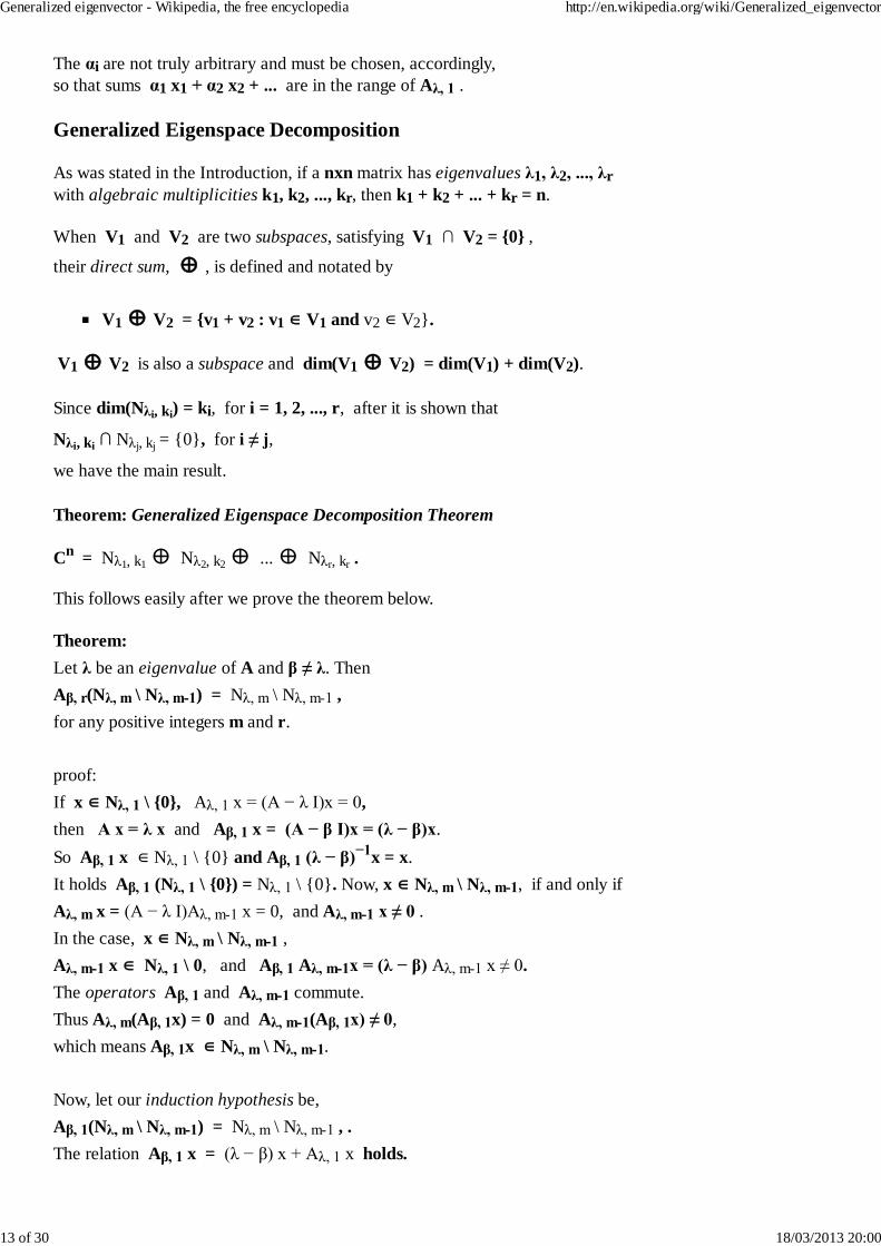
The αi are not truly arbitrary and must be chosen, accordingly,so that sums α1 x1 + α2 x2 + ... are in the range of Aλ, 1 .

Generalized Eigenspace Decomposition

As was stated in the Introduction, if a nxn matrix has eigenvalues λ1, λ2, ..., λrwith algebraic multiplicities k1, k2, ..., kr, then k1 + k2 + ... + kr = n.

When V1 and V2 are two subspaces, satisfying V1 ∩ V2 = {0} ,

their direct sum, ⊕ , is defined and notated by

V1 ⊕ V2 = {v1 + v2 : v1 ∈ V1 and v2 ∈ V2}.

V1 ⊕ V2 is also a subspace and dim(V1 ⊕ V2) = dim(V1) + dim(V2).

Since dim(Nλi, ki) = ki, for i = 1, 2, ..., r, after it is shown that

Nλi, ki ∩ Nλj, kj = {0}, for i ≠ j,

we have the main result.

Theorem: Generalized Eigenspace Decomposition Theorem

Cn = Nλ1, k1 ⊕ Nλ2, k2 ⊕ ... ⊕ Nλr, kr .

This follows easily after we prove the theorem below.

Theorem:Let λ be an eigenvalue of A and β ≠ λ. ThenAβ, r(Nλ, m \ Nλ, m-1) = Nλ, m \ Nλ, m-1 , for any positive integers m and r.

proof:If x ∈ Nλ, 1 \ {0}, Aλ, 1 x = (A − λ I)x = 0, then A x = λ x and Aβ, 1 x = (A − β I)x = (λ − β)x. So Aβ, 1 x ∈ Nλ, 1 \ {0} and Aβ, 1 (λ − β)−1x = x.It holds Aβ, 1 (Nλ, 1 \ {0}) = Nλ, 1 \ {0}. Now, x ∈ Nλ, m \ Nλ, m-1, if and only if Aλ, m x = (A − λ I)Aλ, m-1 x = 0, and Aλ, m-1 x ≠ 0 . In the case, x ∈ Nλ, m \ Nλ, m-1 , Aλ, m-1 x ∈ Nλ, 1 \ 0, and Aβ, 1 Aλ, m-1x = (λ − β) Aλ, m-1 x ≠ 0.The operators Aβ, 1 and Aλ, m-1 commute.Thus Aλ, m(Aβ, 1x) = 0 and Aλ, m-1(Aβ, 1x) ≠ 0,which means Aβ, 1x ∈ Nλ, m \ Nλ, m-1.

Now, let our induction hypothesis be, Aβ, 1(Nλ, m \ Nλ, m-1) = Nλ, m \ Nλ, m-1 , .The relation Aβ, 1 x = (λ − β) x + Aλ, 1 x holds.


13 of 30 18/03/2013 20:00

For y ∈ Nλ, m+1 \ Nλ, m, let x = (λ − β)-1 y + z. Then Aβ, 1 x = y + (λ − β)-1Aλ, 1 y + (λ − β) z + Aλ, 1 z= y + (λ − β)-1Aλ, 1 y + Aβ, 1 z. Now, Aλ, 1 y ∈ Nλ, m \ Nλ, m-1 and, by theinduction hypothesis, there exists z ∈ Nλ, m \ Nλ, m-1 that solves Aβ, 1 z = −(λ − β)-1Aλ, 1 y. It follows x ∈ Nλ, m+1 \ Nλ, m and solves Aβ, 1 x = y.So Aβ, 1(Nλ, m+1 \ Nλ, m) = Nλ, m+1 \ Nλ, m , .

Repeatedly applying Aβ, r = Aβ, 1Aβ, r-1 finishes the proof.

¶

In fact, from the theorem just proved, for i ≠ j,

Aλi, ki(Nλj, kj) = Nλj, kj,.

Now, suppose that Nλi, ki ∩ Nλj, kj ≠ {0}, for some i ≠ j.

Choose x ∈ Nλi, ki ∩ Nλj, kj ≠ 0.

Since x ∈ Nλi, ki , it follows Aλi, ki x = 0.

Since x ∈ Nλj, kj , it follows Aλi, ki x ≠ 0,

because Aλi, ki preserves dimension on Nλj, kj.

So it must be Nλi, ki ∩ Nλj, kj = {0}, for i ≠ j.

This concludes the proof of the Generalized Eigenspace Decomposition Theorem.

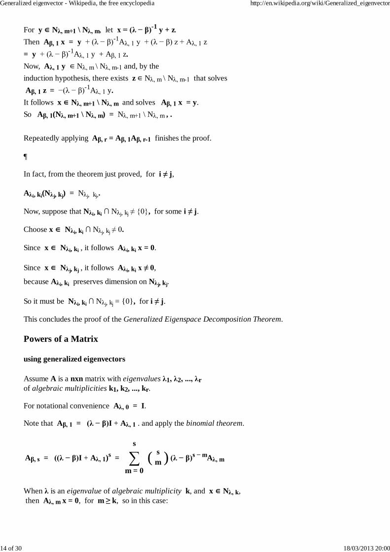
Powers of a Matrix

using generalized eigenvectors

Assume A is a nxn matrix with eigenvalues λ1, λ2, ..., λrof algebraic multiplicities k1, k2, ..., kr.

For notational convenience Aλ, 0 = I.

Note that Aβ, 1 = (λ − β)I + Aλ, 1 . and apply the binomial theorem.

Aβ, s = ((λ − β)I + Aλ, 1)s =

s

∑m = 0

( sm ) (λ − β)s − mAλ, m

When λ is an eigenvalue of algebraic multiplicity k, and x ∈ Nλ, k, then Aλ, m x = 0, for m ≥ k, so in this case:


14 of 30 18/03/2013 20:00

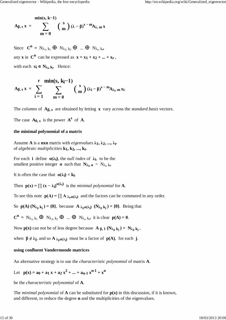
Aβ, s x =

min(s, k−1)

∑m = 0

( sm ) (λ − β)s − mAλ, m x

Since Cn = Nλ1, k1 ⊕ Nλ2, k2 ⊕ ... ⊕ Nλr, kr,

any x in Cn can be expressed as x = x1 + x2 + ... + xr ,

with each xi ∈ Nλi, ki. Hence:

Aβ, s x =

r

∑i = 1

min(s, ki−1)

∑m = 0

( sm ) (λi − β)s − mAλi, m xi.

The columns of Aβ, s are obtained by letting x vary across the standard basis vectors.

The case A0, s is the power As of A.

the minimal polynomial of a matrix

Assume A is a nxn matrix with eigenvalues λ1, λ2, ..., λrof algebraic multiplicities k1, k2, ..., kr.

For each i define α(λi), the null index of λi, to be thesmallest positive integer α such that Nλi, α = Nλi, ki.

It is often the case that α(λi) < ki.

Then p(x) = ∏ (x − λi)α(λi) is the minimal polynomial for A.

To see this note p(A) = ∏ A λi,α(λi) and the factors can be commuted in any order.

So p(A) (Nλj, kj ) = {0}, because A λj,α(λj) (Nλj, kj ) = {0}. Being that

Cn = Nλ1, k1 ⊕ Nλ2, k2 ⊕ ... ⊕ Nλr, kr, it is clear p(A) = 0.

Now p(x) can not be of less degree because A β, 1 (Nλj, kj ) = Nλj, kj ,

when β ≠ λj, and so A λj,α(λj) must be a factor of p(A), for each j.

using confluent Vandermonde matrices

An alternative strategy is to use the characteristic polynomial of matrix A.

Let p(x) = a0 + a1 x + a2 x2 + ... + an-1 xn-1 + xn

be the characteristic polynomial of A.

The minimal polynomial of A can be substituted for p(x) in this discussion, if it is known,and different, to reduce the degree n and the multiplicities of the eigenvalues.


15 of 30 18/03/2013 20:00

Then p(A) = 0 and An = −(a0 I + a1 A + a2 A2 + ... + an-1 An-1).

So An+m = bm, 0 I + bm, 1 A + bm, 2 A2 + ... + bm, n-1 An-1,

where the bm, 0, bm, 1, bm, 2, ..., bm, n-1, satisfy the recurrence relation

bm, 0 = −a0 bm-1, n-1, bm, 1 = bm-1, 0 − a1 bm-1, n-1, bm, 2 = bm-1, 1 − a2 bm-1, n-1, ...,bm, n-1 = bm-1, n-2 − an-1 bm-1, n-1

with b0, 0 = b0, 1 = b0, 2 = ... = b0, n-2 = 0, and b0, n-1 = 1.

This alone will reduce the number of multiplications needed to calculate a higherpower of A by a factor of n2, as compared to simply multiplying An+m by A.

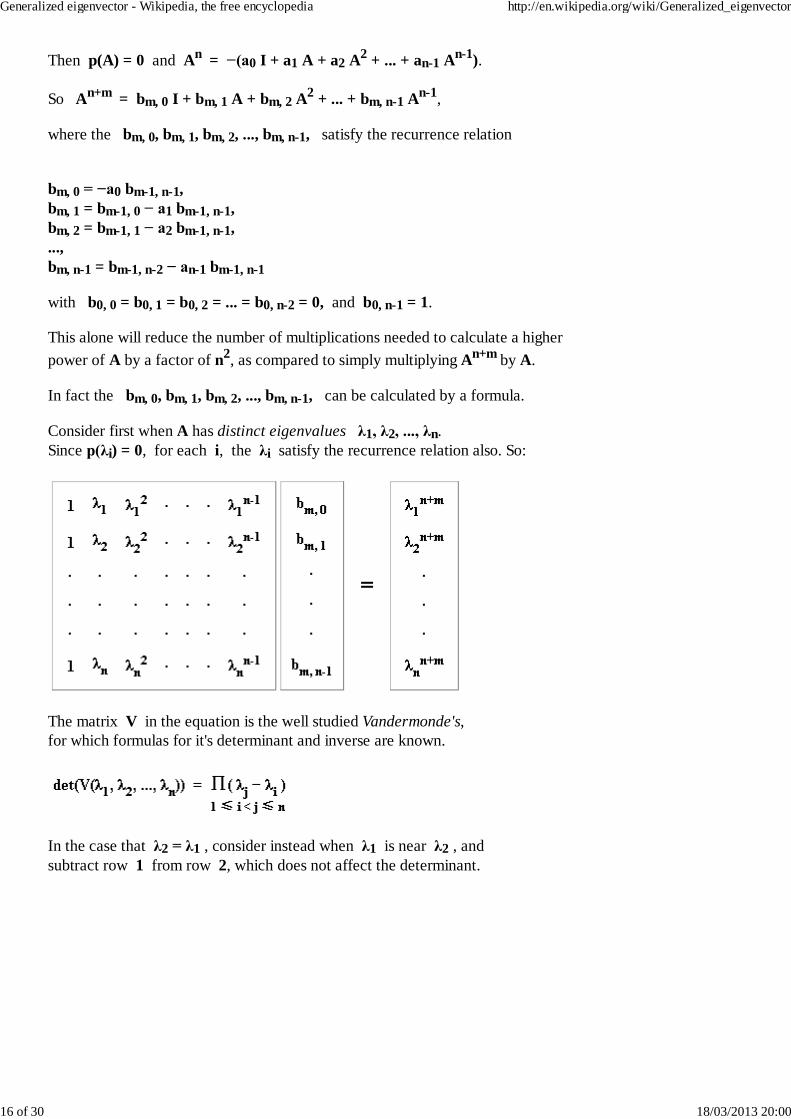
In fact the bm, 0, bm, 1, bm, 2, ..., bm, n-1, can be calculated by a formula.

Consider first when A has distinct eigenvalues λ1, λ2, ..., λn.Since p(λi) = 0, for each i, the λi satisfy the recurrence relation also. So:

The matrix V in the equation is the well studied Vandermonde's,for which formulas for it's determinant and inverse are known.

In the case that λ2 = λ1 , consider instead when λ1 is near λ2 , andsubtract row 1 from row 2, which does not affect the determinant.


16 of 30 18/03/2013 20:00

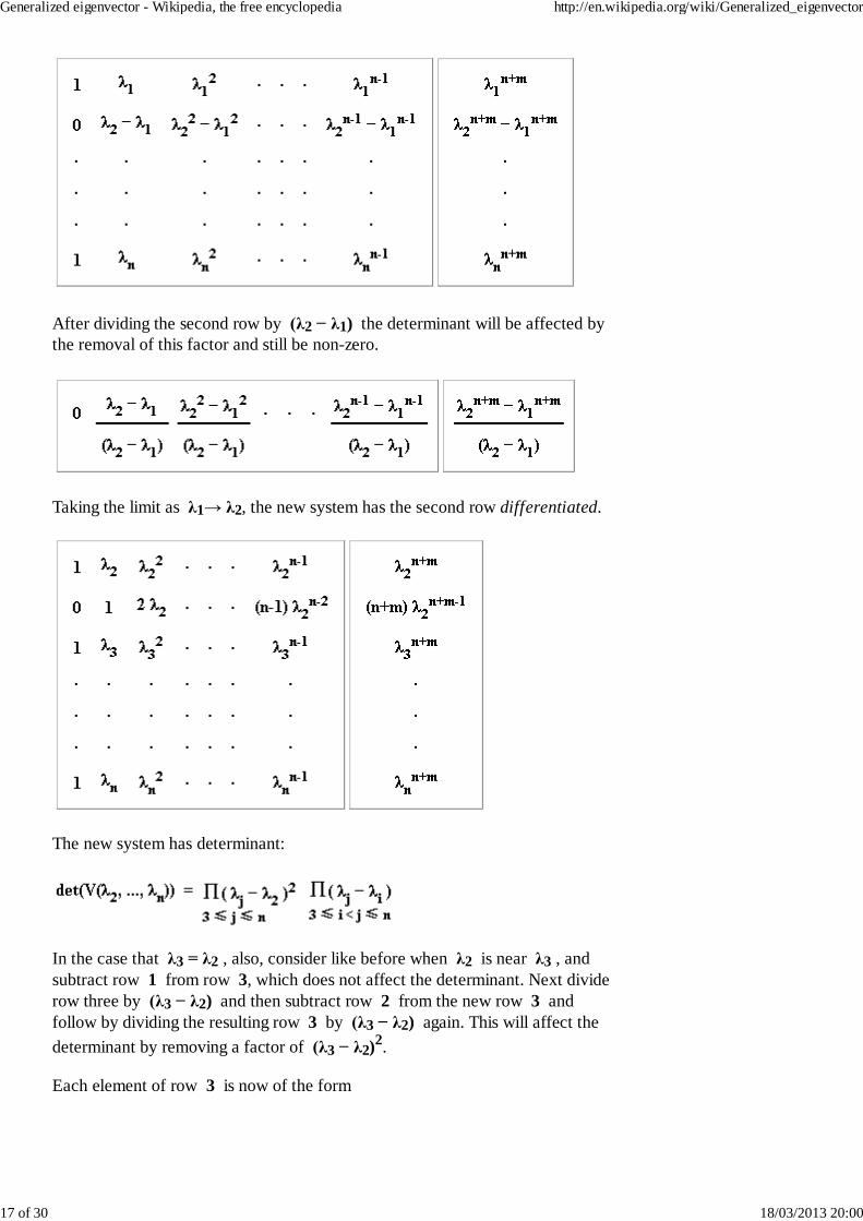
After dividing the second row by (λ2 − λ1) the determinant will be affected bythe removal of this factor and still be non-zero.

Taking the limit as λ1→ λ2, the new system has the second row differentiated.

The new system has determinant:

In the case that λ3 = λ2 , also, consider like before when λ2 is near λ3 , andsubtract row 1 from row 3, which does not affect the determinant. Next dividerow three by (λ3 − λ2) and then subtract row 2 from the new row 3 andfollow by dividing the resulting row 3 by (λ3 − λ2) again. This will affect thedeterminant by removing a factor of (λ3 − λ2)2.

Each element of row 3 is now of the form


17 of 30 18/03/2013 20:00

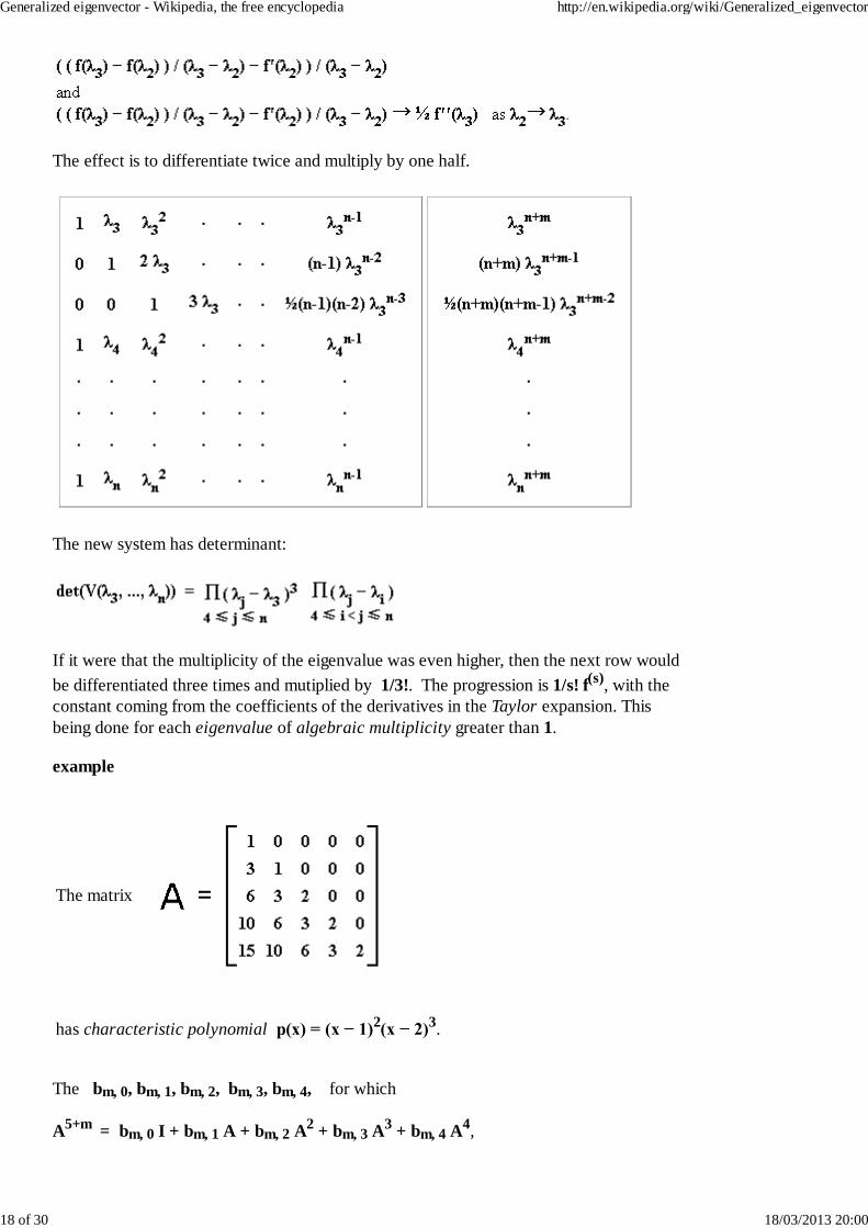
The effect is to differentiate twice and multiply by one half.

The new system has determinant:

If it were that the multiplicity of the eigenvalue was even higher, then the next row wouldbe differentiated three times and mutiplied by 1/3!. The progression is 1/s! f(s), with theconstant coming from the coefficients of the derivatives in the Taylor expansion. Thisbeing done for each eigenvalue of algebraic multiplicity greater than 1.

example

The matrix

has characteristic polynomial p(x) = (x − 1)2(x − 2)3.

The bm, 0, bm, 1, bm, 2, bm, 3, bm, 4, for which

A5+m = bm, 0 I + bm, 1 A + bm, 2 A2 + bm, 3 A3 + bm, 4 A4,


18 of 30 18/03/2013 20:00

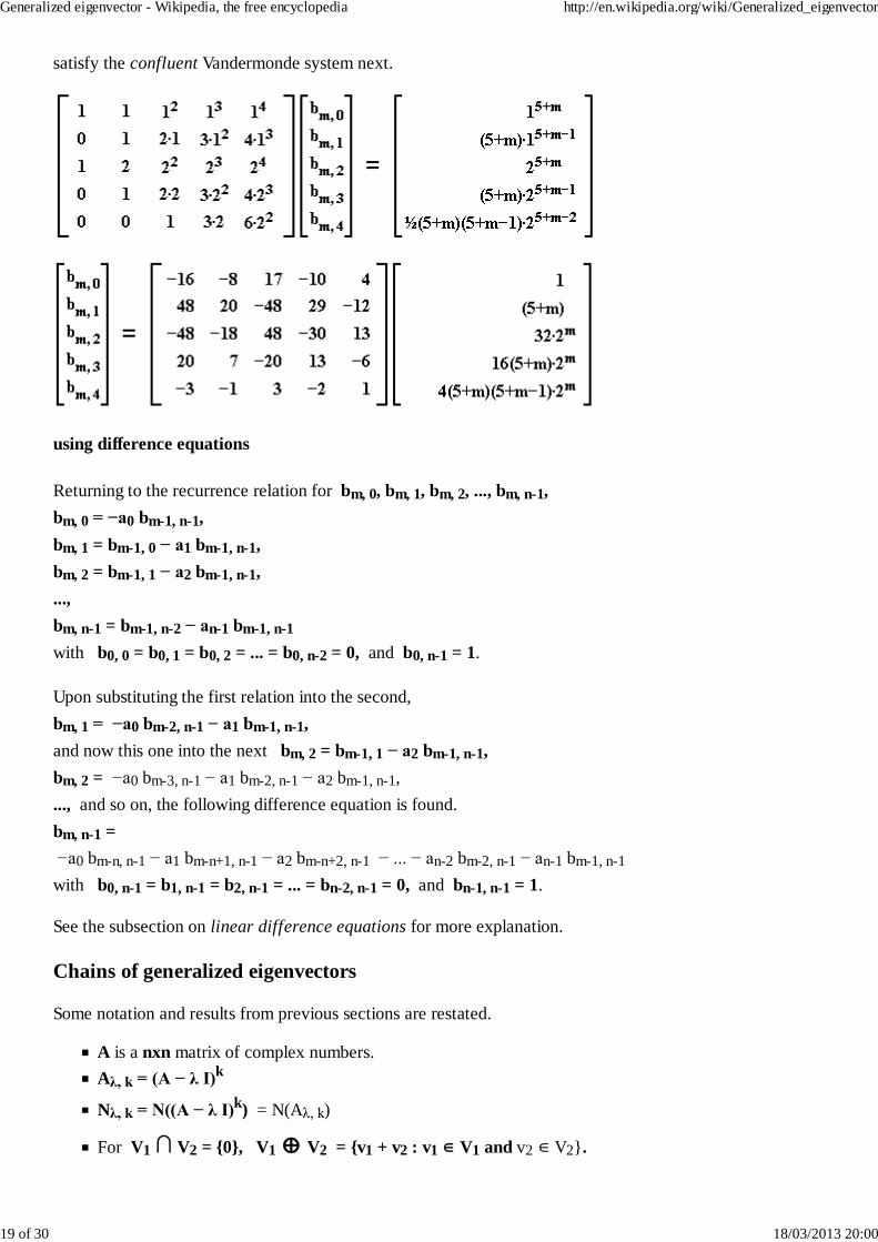
satisfy the confluent Vandermonde system next.

using difference equations

Returning to the recurrence relation for bm, 0, bm, 1, bm, 2, ..., bm, n-1,bm, 0 = −a0 bm-1, n-1, bm, 1 = bm-1, 0 − a1 bm-1, n-1, bm, 2 = bm-1, 1 − a2 bm-1, n-1, ...,bm, n-1 = bm-1, n-2 − an-1 bm-1, n-1

with b0, 0 = b0, 1 = b0, 2 = ... = b0, n-2 = 0, and b0, n-1 = 1.

Upon substituting the first relation into the second,bm, 1 = −a0 bm-2, n-1 − a1 bm-1, n-1, and now this one into the next bm, 2 = bm-1, 1 − a2 bm-1, n-1, bm, 2 = −a0 bm-3, n-1 − a1 bm-2, n-1 − a2 bm-1, n-1, ..., and so on, the following difference equation is found.bm, n-1 = −a0 bm-n, n-1 − a1 bm-n+1, n-1 − a2 bm-n+2, n-1 − ... − an-2 bm-2, n-1 − an-1 bm-1, n-1

with b0, n-1 = b1, n-1 = b2, n-1 = ... = bn-2, n-1 = 0, and bn-1, n-1 = 1.

See the subsection on linear difference equations for more explanation.

Chains of generalized eigenvectors

Some notation and results from previous sections are restated.

A is a nxn matrix of complex numbers.Aλ, k = (A − λ I)k

Nλ, k = N((A − λ I)k) = N(Aλ, k)

For V1 ∩ V2 = {0}, V1 ⊕ V2 = {v1 + v2 : v1 ∈ V1 and v2 ∈ V2}.


19 of 30 18/03/2013 20:00

Assume A has eigenvalues λ1, λ2, ..., λrof algebraic multiplicities k1, k2, ..., kr.

For each i define α(λi), the null index of λi, to be thesmallest positive integer α such that Nλi, α = Nλi, ki.

It is always the case that α(λi) ≤ ki.

When α(λ) ≥ 2 ,

Nλ, 1 ⊂ Nλ, 2 ⊂ ... ⊂ Nλ, α-1 ⊂ Nλ, α = Nλ, α+1 = ...,

Nλ, α \ {0} = ∪ (Nλ, m \ Nλ, m-1), for m = 1, ..., α and Nλ, 0 = {0}.

x ∈ Nλ, m \ Nλ, m-1, if and only if Aλ, 1 x ∈ Nλ, m-1 \ Nλ, m-2

Define a chain of generalized eigenvectors to be a set{ x1, x2, ..., xm } such that x1 ∈ Nλ, m \ Nλ, m-1, and xi+1 = Aλ, 1 xi.

Then xm ≠ 0 and Aλ, 1 xm = 0.

When x1 ∈ Nλ, 1 \ {0}, {x1} can be, for the sake of not requiring extraterminology, considered trivially a chain.

When a disjoint collection of chains combined form a basis set for Nλ, α(λ) ,they are often referred to as Jordan chains and are the vectors used forthe columns of a transformation matrix in the Jordan canonical form.

When a disjoint collection of chains that combined form a basis set,is needed that satisfy βi+1xi+1 = Aλ, 1 xi, for some scalars βi, chainsas already defined can be scaled for this purpose.

What will be proven here is that such a disjoint collection of chainscan always be constructed.

Before the proof is started, recall a few facts about direct sums.

When the notation V1 ⊕ V2 is used, it is assumed V1 ∩ V2 = {0}.

For x = v1 + v2 with v1 ∈ V1 and v2 ∈ V2 , then x = 0,

if and only if v1 = v2 = 0.

In the discussion belowδi = dim(Nλ, i) − dim(Nλ, i−1), with δ1 = dim(Nλ, 1).

First consider when Nλ, 2 \ Nλ, 1 ≠ {0} , Then a basis for Nλ, 1 can be

extended to a basis for Nλ, 2. If δ2 = 1, then there exists x1 ∈ Nλ, 2 \ Nλ, 1,

such that Nλ, 2 = Nλ, 1 ⊕ span{x1}. Let x2 = Aλ, 1 x1. Then

x2 ∈ Nλ, 1 \ {0}, with x1 and x2 linearly independent. If dim(Nλ, 2) = 2,

since {x1, x2} is a chain we are through. Otherwise x1, x2 can be extended

to a basis x1, x2, ..., xδ1 for Nλ, 2. The sets {x1, x2}, {x3}, ..., {xδ1}

form a disjoint collection of chains. In the case that δ2 > 1, then there exist


20 of 30 18/03/2013 20:00

linearly independent x1, x2, ..., xδ2 ∈ Nλ, 2 \ Nλ, 1, such that

Nλ, 2 = Nλ, 1 ⊕ span{x1, x2, ..., xδ2}. Let yi = Aλ, 1 xi.

Then yi ∈ Nλ, 1 \ {0}, for i = 1, 2, ..., δ2. To see the y1, y2, ..., yδ2

are linearly independent, assume that for some β1, β2, ..., βδ2,

that β1y1 + β2y2 + ... + βδ2yδ2 = 0, Then for x = β1x1 + β2x2 + ... + βδ2xδ2,

x ∈ Nλ, 1 , and x ∈ span{x1, x2, ..., xδ2}, which implies that x = 0, and

β1= β2= ... = βδ2 = 0. Since span{y1, y2, ..., yδ2} ⊆ Nλ, 1, the vectors

x1, x2, ..., xδ2 , y1, y2, ..., yδ2 are a linearly independent set.

If δ2 = δ1, then the sets {x1, y1}, {x2, y2}, ..., {xδ2, yδ2} form a

disjoint collection of chains that when combined are a basis set for Nλ, 2.

If δ1 > δ2, then x1, x2, ..., xδ2 , y1, y2, ..., yδ2 can be extended to a basis

for Nλ, 2 by some vectors xδ2+1, ..., xδ1 in Nλ, 1, so that

{x1, y1}, {x2, y2}, ..., {xδ2, yδ2} , {xδ2+1}, ..., {xδ1}

forms a disjoint collection of chains.

To reduce redundancy, in the next paragraph, when δ = 1 the notationx1, x2, ..., xδ will be understood simply to mean just x1 and when δ = 2 to mean x1, x2.

So far it has been shown that, if linearly independent

x1, x2, ..., xδ2 ∈ Nλ, 2 \ Nλ, 1, are chosen, such that

Nλ, 2 = Nλ, 1 ⊕ span{x1, x2, ..., xδ2}, then there exists a disjoint

collection of chains with each of the x1, x2, ..., xδ2 being the first member or top

of one of the chains. Furthermore, this collection of vectors, when combined,

forms a basis for Nλ, 2.

Now, let the induction hypothesis be that, if linearly independent

x1, x2, ..., xδm ∈ Nλ, m \ Nλ, m−1, are chosen, such that

Nλ, m = Nλ, m−1 ⊕ span{x1, x2, ..., xδm}, then there exists a disjoint

collection of chains with each of the x1, x2, ..., xδm being the first member or top


forms a basis for Nλ, m.

Consider m < α(λ). A basis for Nλ, m can always be extended to a basis for

Nλ, m+1. So linearly independent x1, x2, ..., xδm+1 ∈ Nλ, m+1 \ Nλ, m, such that

Nλ, m+1 = Nλ, m ⊕ span{x1, x2, ..., xδm+1}, can be chosen. Let yi = Aλ, 1 xi.

Then yi ∈ Nλ, m \ Nλ, m−1, for i = 1, 2, ..., δm+1. To see the y1, y2, ..., yδm+1

are linearly independent, assume that for some β1, β2, ..., βδm+1,


21 of 30 18/03/2013 20:00

that β1y1 + β2y2 + ... + βδm+1yδm+1 = 0, Then for

x = β1x1 + β2x2 + ... + βδm+1xδm+1, x ∈ Nλ, 1 , and

x ∈ span{x1, x2, ..., xδm+1}, which implies that x = 0, and

β1= β2= ... = βδm+1 = 0. In addition, span{y1, y2, ..., yδm+1} ∩ Nλ, m−1 = {0}.

To see this assume that for some β1, β2, ..., βδm+1,

that β1y1 + β2y2 + ... + βδm+1yδm+1 ∈ Nλ, m−1 Then for

x = β1x1 + β2x2 + ... + βδm+1xδm+1, x ∈ Nλ, m , and

x ∈ span{x1, x2, ..., xδm+1}, which implies that x = 0, and

β1= β2= ... = βδm+1 = 0. The proof is nearly done.

At this point suppose that b1, b2, ..., bdm−1 is any basis for Nλ, m−1.

Then B = span{b1, b2, ..., bdm−1} ⊕ span{y1, y2, ..., yδm+1}

is a subspace of Nλ, m. If B ≠ Nλ, m, then

b1, b2, ..., bdm−1, y1, y2, ..., yδm+1 can be extended to a basis for Nλ, m,

by some set of vectors z1, z2, ..., z(δm− δm+1) , in which case

Nλ, m = Nλ, m−1 ⊕ span{y1, y2, ..., yδm+1} ⊕ span{z1, z2, ..., z(δm− δm+1)}.

If δm = δm+1, then

Nλ, m = Nλ, m−1 ⊕ span{y1, y2, ..., yδm+1}

or if δm > δm+1, then

Nλ, m = Nλ, m−1 ⊕ span{z1, z2, ..., z(δm− δm+1) , y1, y2, ..., yδm+1}

In either case apply the induction hypothesis to get that there exists a disjoint

collection of chains with each of the y1, y2, ..., yδm+1 being the first member or top


forms a basis for Nλ, m. Now, yi = Aλ, 1 xi, for i = 1, 2, ..., δm+1, so each of the

chains beginning with yi can be extended upwards into Nλ, m+1 \ Nλ, m to a chain

beginning with xi. Since Nλ, m+1 = Nλ, m ⊕ span{x1, x2, ..., xδm+1},

the combined vectors of the new chains form a basis for Nλ, m+1.

Differential equations y′= Ay

Let A be a n×n matrix of complex numbers and λ an eigenvalue of A , with

associated eigenvector x . Suppose y(t) is a n dimensional vector valued

function, sufficiently smooth, so that y′(t) is continuous. The restriction that y(t)

be smooth can be relaxed somewhat, but is not the main focus of this discussion.

The solutions to the equation y′(t) = Ay(t) are sought. The first observation is that y(t) = eλtx will be a solution. When A does not have n linearly independent


22 of 30 18/03/2013 20:00

eigenvectors, solutions of this kind will not provide the total of n needed for afundamental basis set.

In view of the existence of chains of generalized eigenvectors seek a solution of

the form 'y(t) = eλtx1 + t'eλtx2 , then

y′(t) =' λ eλtx1 + eλtx2 + λ t eλtx2 =' eλt(λ x1 + x2)'''' + t eλt(λx 2)

and

Ay(t) = eλtA x1 + t eλtA x2 .

In view of this, y(t) will be a solution to y′(t) = Ay(t) , when 'A x1 = λ x1 + x2' and

A x2 = λ x2 . That is when (A − λ I)x1 = x2 and (A − λ I)x2 = 0 . Equivalently,

when {x1, x2} is a chain of generalized eigenvectors.

Continuing with this reasoning seek a solution of the form

y(t) = eλtx1 + t eλtx2 + t2 eλtx3 , then

y′(t) = λ eλtx1 + eλtx2 + λ t eλtx2 + 2 t eλtx3 + λ t2 eλtx3

= eλt(λ x1 + x2) + t eλt(λ x2 + 2 x3) + t2 eλt(λ x3)' and

Ay(t) = eλtA x1 + t eλtA x2 + t2 eλtA x3 .

Like before, y(t) will be a solution to y′(t) = Ay(t) , when 'A x1 = λ x1 + x2' , 'A x2 = λ x2 + 2 x3' , and A x3 = λ x3 . That is when (A − λ I)x1 = x2 , (A − λ I)x2 = 2 x3 , and (A − λ I)x3 = 0 . Since it will hold (A − λ I)(2 x3) = 0 ,also, equivalently, when {x1, x2, 2 x3} is a chain of generalized eigenvectors.

More generally, to find the progression, seek a solution of the form

y(t) = eλtx1 + t eλtx2 + t2 eλtx3 + t3 eλtx4 + ... + tm−2 eλtxm−1 + tm−1 eλtxm ,

then

y′(t) = λ eλtx1 + eλtx2 + λ t eλtx2' + 2 t eλtx3' + λ t2 eλtx3' + 3 t2 eλtx4' + λ t3 eλtx4'

+ ...' + (m−2)tm−3eλtxm−1' + λ tm−2 eλtxm−1' + (m−1)tm−2 eλtxm' + λ tm−1 eλtxm

=' eλt(λ x1 + x2) + t eλt(λ x2 + 2 x3) + t2 eλt(λ x3 + 3 x4) + t3 eλt(λ x4 + 4 x5)

+ ...

+ tm−3 eλt(λ xm−2 + (m−2) xm−1) + tm−2 eλt(λ xm−1 + (m−1) xm) + tm−1 eλt(λ xm)'

and

Ay(t) =

eλtA x1 + t eλtA x2 + t2 eλtA x3 + t3 eλtA x4 + ... + tm−2 eλtA xm−1 + tm−1 eλtA xm .

Again, y(t) will be a solution to y′(t) = Ay(t) , when

'A x1 = λ x1 + x2' , A x2 = λ x2 + 2 x3 , A x3 = λ x3 + 3 x4 , A x4 = λ x4 + 4 x5 ,

A xm−2 = λ xm−2 + (m−2) xm−1 , A xm−1 = λ xm−1 + (m−1) xm ,


23 of 30 18/03/2013 20:00

and A xm = λ xm .

That is when

(A − λ I)x1 = x2 , (A − λ I)x2 = 2 x3 , (A − λ I)x3 = 3 x4 , (A − λ I)x4 = 4 x5 ,

...,

(A − λ I)xm−2 = (m−2) xm−1 , (A − λ I)xm−1 = (m−1) xm , and

(A − λ I)xm = 0 .

Since it will hold (A − λ I)((m−1)! x3) = 0 , also, equivalently, when

{x1, 1! x2, 2! x3, 3! x4, ..., (m−2)! xm−1, (m−1)! xm}

is a chain of generalized eigenvectors.

Now, the basis set for all solutions will be found through a disjoint collectionof chains of generalized eigenvectors of the matrix A.

Assume A has eigenvalues λ1, λ2, ..., λr

of algebraic multiplicities k1, k2, ..., kr.

For a given eigenvalue λi there is a collection of s, with s depending on i,

disjoint chains of generalized eigenvectors

Ci,1 = {1z1, 1z2, ...,1zj1}, Ci,2 = {2z1, 2z2, ...,2zj2}, ..., Ci,js(i) = {sz1, sz2, ...,szjs},

that when combined form a basis set for Nλi, ki. The total number of vectors

in this set will be j1 + j2 + ... + js = ki. Sets in this collection may have only one

or two members so in this discussion understand the notation {βz1, βz2, ...,βzjβ}

will mean {βz1} when jβ = 1, and {βz1, βz2} when jβ = 2, and so forth.

Being that this notation is cumbersome with many indices, in the next paragraphsany particular Ci,β, when more explanation is not needed, may just be notated asC = {z1, z2, ..., zj}.

For each such of these chain sets, C = {z1, z2, ..., zj}the sets {xj}, {xj−1, xj}, {xj−2, xj−1, xj}, ..., {z2, z3, ..., zj}, {z1, z2, ..., zj}are also chains. This notation being understood to mean whenC = {z1} just {z1}, when C = {z1, z2} just {z2}, {z1, z2} and whenC = {z1, z2, z2} just {z3}, {z2, z3}, {z1, z2, z3}, and so on.

The conclusion of the top of the discussion was that

y(t) = eλtx1, is a solution when {x1} is a chain.

y(t) = eλtx1 + t eλtx2, is a solution when {x1, 1! x2} is a chain.

y(t) = eλtx1 + t eλtx2 + t2 eλtx3, is a solution when {x1, 1! x2, , 2! x3} is a chain.

The progression continues to

y(t) = eλtx1 + t eλtx2 + t2 eλtx3 + t3 eλtx4 + ... + tm−2 eλtxm−1 + tm−1 eλtxm,


24 of 30 18/03/2013 20:00

is a solution when {x1, 1! x2, 2! x3, 3! x4, ..., (m−2)! xm−1, (m−1)! xm},

is a chain of generalized eigenvectors.

In light of the preceding calculations, all that must be done is to provide the proper

scaling for each of the chains arising from the set C = {z1, z2, ..., zj}.

The progression for the solutions is given by

y(t) = eλtzj, for chain {zj}

y(t) = eλtzj−1 + (1 ⁄ 1!) t eλtzj, for chain {zj−1, 1!(1 ⁄ 1!) zj}

y(t) = eλtzj−2 + (1 ⁄ 1!) t eλtzj−1 + (1 ⁄ 2!) t2 eλtzj,

for chain {zj−2, 1!(1 ⁄ 1!) zj−1, 2!(1 ⁄ 2!) zj}

y(t) = eλtzj−3 + (1 ⁄ 1!) t eλtzj−2 + (1 ⁄ 2!) t2 eλtzj−1 + (1 ⁄ 3!) t3 eλtzj,

for chain {zj−3, 1!(1 ⁄ 1!) zj−2, 2!(1 ⁄ 2!) zj−1, 3!(1 ⁄ 3!) zj},

and so on until,

y(t) = eλtz1 + (1 ⁄ 1!) t eλtz2 + (1 ⁄ 2!) t2 eλtz3 + ... + (1 ⁄ (j−1)!) t j−1 eλtzj,

for the chain of generalized eigenvectors,

{z1, 1!(1 ⁄ 1!) z2, 2!(1 ⁄ 2!) z3, ..., (j−2)!(1 ⁄ (j−2)!) xj−1, (j−1)!(1 ⁄ (j−1)!) zj}.

What is left to show is that when all the solutions constructed from the chain sets,as described, are considered, they form a fundamental set of solutions.To do this it has to be shown that there are n of them and that they arelinearly independent.

Reiterating, for a given eigenvalue λi there is a collection of s, with s depending on i,

disjoint chains of generalized eigenvectors

Ci,1 = {1z1, 1z2, ...,1zj1(i)}, Ci,2 = {2z1, 2z2, ...,2zj2(i)},

..., Ci,js(i) = {s(i)z1, s(i)z2, ...,s(i)zjs(i)},

that when combined form a basis set for Nλi, ki. The total number of vectors

in this set will be j1(i) + j2(i) + ... + js(i) = ki.

Thus the total number of all such basis vectors and so solutions isk1 + k2 + ... + kr = n.

Each solution is one of the forms y(t) = eλtx1, y(t) = eλtx1 + t eλtx2,

y(t) = eλtx1 + t eλtx2 + t2 eλtx3, y(t) = eλtx1 + t eλtx2 + t2 eλtx3 + ....

Now each basis vector vj, for j = 1, 2, ..., n; of the combined set of

generalized eigenvectors, occurs as x1 in one of the expressions immediately

above precisely once. That is, for each j, there is one yj(t) = eλtvj + ...

Since yj(0) = eλ0vj = vj, the set of solutions are linearly independent at t = 0.

Revisiting the powers of a matrix


25 of 30 18/03/2013 20:00

As a notational convenience Aλ, 0 = I.

Note that A = λ I + Aλ, 1 . and apply the binomial theorem.

As = (λ I + Aλ, 1)s =

s

∑r = 0

( sr ) λs − rAλ, r

Assume λ is an eigenvalue of A, and let { x1, x2, ..., xm }

be a chain of generalized eigenvectors such that x1 ∈ Nλ, m \ Nλ, m-1 ,

xi+1 = Aλ, 1 xi ,. xm ≠ 0 , and Aλ, 1 xm = 0.

Then xr+1 = Aλ, r x1, for r = 0, 1, ..., m-1.

As x1 =

s

∑r = 0

( sr ) λs − rAλ, r x1 =

s

∑r = 0

( sr ) λs − r xr+1

So for s ≤ m − 1

As x1 =

s

∑r = 0

( sr ) λs − r xr+1

and for s ≥ m − 1, since Aλ, m x1 = 0,

As x1 =

m −1

∑r = 0

( sr ) λs − r xr+1 .

Ordinary linear difference equations

Ordinary linear difference equations are equations of the sort:yn = a yn−1 + byn = a yn−1 + b yn−2 + cor more generally,yn = amyn−1 + am−1yn−2 + ... + a2yn−m + 1 + a1yn−m + a0

with initial conditionsy0, y1, y2, ..., ym−2, ym−1.

A case with a1 = 0 can be excluded, since it represents an equation of less degree.

They have a characteristic polynomial

p(x) = xm − amxm−1 − am−1xm−2 − ... − a2x − a1.


26 of 30 18/03/2013 20:00

To solve a difference equation it is first observed, if yn and zn are both solutions,

then (yn − zn) is a solution of the homogeneous equation:

yn = amyn−1 + am−1yn−2 + ... + a2yn−m + 1 + a1yn−m.

So a particular solution to the difference equation must be found together withall solutions of the homogeneous equation to get the general solution for thedifference equation. Another observation to make is that, if yn is a solution tothe inhomogeneous equation, thenzn = yn+1 − ynis also a solution to the homogeneous equation.So all solutions of the homogeneous equation will be found first.

When β is a root of p(x) = 0, then it is easily seen

yn = βn is a solution to the homogeneous equation since

yn − amyn−1 − am−1yn−2 − ... − a2yn−m + 1 − a1yn−m,

becomes upon the substitution yn = βn,

βn − amβn−1 − am−1βn−2 − ... − a2βn−m + 1 − a1βn−m

= βn−m(βm − amβm−1 − am−1βm−2 − ... − a2β − a1)

= βn−mp(β) = 0.

When β is a repeated root of p(x) = 0, then

yn = nβn−1 is a solution to the homogeneous equation since

nβn−1 − am(n−1)βn−2 − am−1(n−2)βn−3 − ... − a2(n−m + 1)βn−m − a1(n−m)βn−m − 1

= (n−m)βn−m − 1(βm − amβm−1 − am−1βm−2 − ... − a2β − a1)

+ βn−m − 1(mβm−1 − (m−1)amβm−2 − (m−2)am−1βm−3 − ... − 2a3β − a2)

== (n−m)βn−m − 1p(β) + βn−m − 1p′(β) == 0.

After reaching this point in the calculation the mystery is solved. Just notice when

β is a root of p(x) = 0 with mutiplicity k, then for s = 1, 2, ..., k−1

ds(βn−mp(β))/dβs = 0.

Referring this back to the original equation

βn − amβn−1 − am−1βn−2 − ... − a2βn−m + 1 − a1βn−m

it is seen that

yn = ds(βn)/dβs

are solutions to the homogeneous equation. For example, if β is a root of

multiplicity 3, then yn = n(n−1)βn−2 is a solution. In any case this gives m

linearly independent solutions to the homogeneous equation.

To look for a particular solution first consider the simpliest equation.


27 of 30 18/03/2013 20:00

yn = a yn−1 + b.

It has a particular solution yp,n given by

yp,0 = 0, yp,1 = b, yp,2 = (1 + a)b, ..., yp,n = (1 + a + a2 + ... + an−1)b, ..., .

It's homogeneous equation yn = a yn−1 has solutions yn = any0.

So zn = yn+1 − yn = anb

can be telescoped to get

yn = (yn − yn−1) + (yn−1 − yn−2) + ... + (y2 − y1) + (y1 − y0) + y0

= zn−1 + zn−2 + ... + z1 + z0 + y0

= (1 + a + a2 + ... + an−1)b ,

the particular solution with y0 = 0.

Now, returning to the general problem, the equationyn = amyn−1 + am−1yn−2 + ... + a2yn−m + 1 + a1yn−m + a0.When yp,n is a particular solution with yp,0 = 0, then zn = yp,n+1 − yp,n is a solution to the homogeneous equation with z0 = yp,1 .So zn = yp,n+1 − yp,n can be telescoped to getyp,n = (yp,n − yp,n−1) + (yp,n−1 − yp,n−2) + ... + (yp,2 − yp,1) + (yp,1 − yp,0) + yp,0= zn−1 + zn−2 + ... + z1 + z0 Consideringyp,m = amyp,m−1 + am−1yp,m−2 + ... + a2yp,1 + a1yp,0 + a0.and rewriting the equation in the zizm−1 + zm−2 + ... + z1 + z0 = (am) ( zm−2 + zm−3 + ... + z1 + z0) + (am−1) ( zm−3 + zm−4 + ... + z1 + z0) + (am−2) ( zm−4 + zm−5 + ... + z1 + z0) + · · · + (a3) ( z1 + z0) + (a2) ( z0) + (a0)andzm−1

= (am − 1) zm−2 + (am + am−1 − 1) zm−3 + (am + am−1 + am−2 − 1) zm−4

+ · · · + (am + am−1 + ... + a4 + a3 − 1) z1 + (am + am−1 + ... + a3 + a2 − 1) z0

+ (a0).

Since a solution of the homogeneous equation can be found for any initial conditionsz0, z1, z2, ..., zm−2, zm−1.reasoning conversely find such zi satisfying the equation,just before and define yp,n by the relation yp,0 = 0, yp,n = zn−1 + zn−2 + ... + z1 + z0


28 of 30 18/03/2013 20:00

One choice is, for example, zm−1 = a0, z0 = z1 = z2 = ... = zm−2 = 0.This solution solves the problem for all initial values equal to zero.

The general solution to the inhomogeneous equation is given byyn = yp,n + γ1 w(1)n + γ2 w(2)n + ... + γm−1 w(m−1)n + γm w(m)nwherew(1)n, w(2)n, ..., w(m−1)n, w(m)nare a basis for the homogeneous equation, andγ1, γ2, ..., γm−1, γmare scalars.

example

yn = 8 yn−1 − 25 yn−2 + 38 yn−3 − 28 yn−4 + 8 yn−5 + 1with initial conditionsy0 = 0, y1 = 0, y2 = 0, y3 = 0, and y4 = 0.

The characteristic polynomial for the equation is

p(x) = x5 − 8x4 + 25x3 − 38x2 + 28x − 8 = (x − 1)2(x − 2)3.

The homogeneous equation has independent solutions

w1n = 1n = 1, w2n = n·1n−1 = n, and

w3n = 2n, w4n = n·2n−1, w5n = n(n−1)·2n−2.

The solution to the homogeneous equation

zn = −3 w1n − w2n + 3 w3n − 2 w4n + ½ w5n

satisfies the initial conditions

z4 = 1, z0 = z1 = z2 = z3 = 0.

A particular solution can be found by

yp,0 = 0, yp,n = zn−1 + zn−2 + ... + z1 + z0 .

Calculating sums:

∑w1 = w1n−1 + w1n−2 + ... + w11 + w10 = n .

∑w2 = w2n−1 + w2n−2 + ... + w21 + w20 = (n−1)n / 2 .

∑w3 = w3n−1 + w3n−2 + ... + w31 + w30 = 2n − 1 .

Sums of these kinds are found by differentiating (xn − 1) / (x − 1).

∑w4 = w4n−1 + w4n−2 + ... + w41 + w40 = (n−2)2n−1 + 1 .

∑w5 = w5n−1 + w5n−2 + ... + w51 + w50 = (n2 − 5n + 8)2n−2 − 2 .

Now,

yp,n = −3 ∑w1n − ∑w2n + 3 ∑w3n − 2 ∑w4n + ½ ∑w5n

solves the initial value problem of this example.


29 of 30 18/03/2013 20:00

At this point it is worthwhile to notice that all the terms that are combinations of

scalar multiples of basis elements can be removed. These are any multiples of

1, n, 2n, n·2n−1, and n2·2n−2.

So instead the particular solution next, may be preferred.

yp,n = −½ n2 .

This solution has non zero initial values, which must be taken into account.

y0 = 0, y1 = −1 ⁄ 2, y2 = −2, y3 = −9 ⁄ 2, and y4 = −8.

References

Axler, Sheldon (1997). Linear Algebra Done Right (2nd ed.). Springer. ISBN 978-0-387-98258-8.

Retrieved from "http://en.wikipedia.org/w/index.php?title=Generalized_eigenvector&oldid=544346744"Categories: Linear algebra

This page was last modified on 15 March 2013 at 11:25.Text is available under the Creative Commons Attribution-ShareAlike License; additional terms mayapply. See Terms of Use for details.Wikipedia® is a registered trademark of the Wikimedia Foundation, Inc., a non-profit organization.


30 of 30 18/03/2013 20:00

Generalized eigenvectorpmh/teach/algebra/additional/eigen.pdf · 2013-03-18 · that this matrix is...

Documents

Transcript of Generalized eigenvectorpmh/teach/algebra/additional/eigen.pdf · 2013-03-18 · that this matrix is...