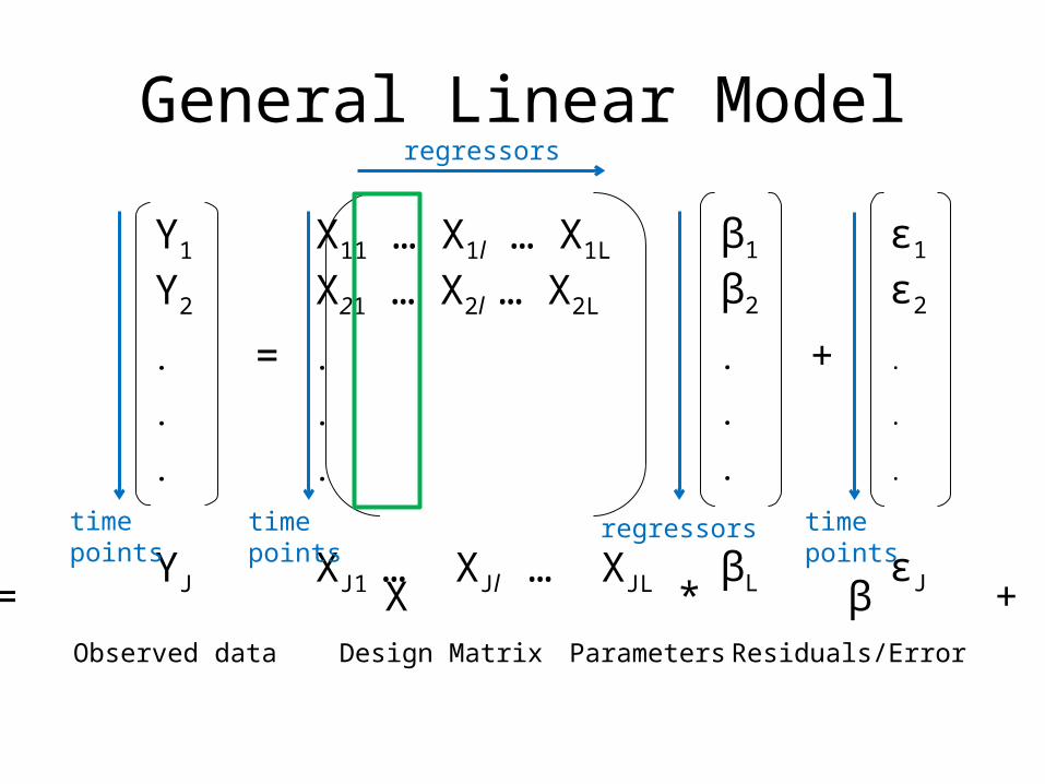
General Linear Model. Y1Y2...YJY1Y2...YJ = X 11 … X 1l … X 1L X 21 … X 2l … X 2L. X J1 … X...
31
General Linear Model
-
Upload
charles-dalton -
Category
Documents
-
view
222 -
download
1
Transcript of General Linear Model. Y1Y2...YJY1Y2...YJ = X 11 … X 1l … X 1L X 21 … X 2l … X 2L. X J1 … X...

General Linear Model
General Linear Model
Y1
Y2
.
.
.
YJ
=
X11 … X1l … X1L
X21 … X2l … X2L
.
.
.
XJ1 … XJl … XJL
β1
β2
.
.
.
βL
+
ε1
ε2
.
.
.
εJY = X * β + ε
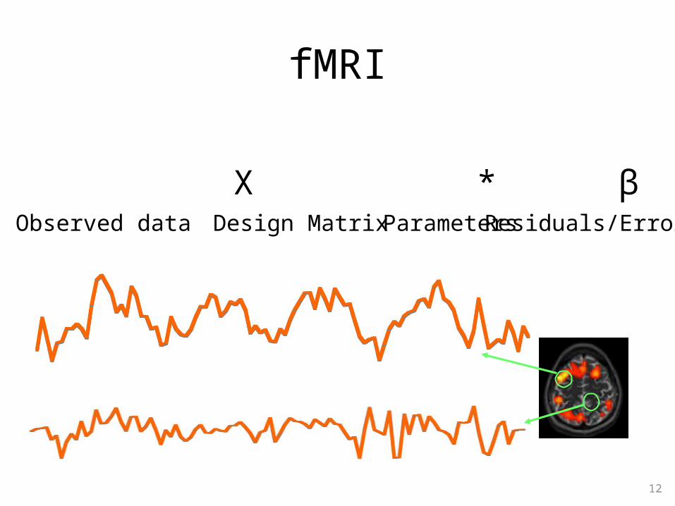
Observed data Design Matrix Parameters Residuals/Error
timepoints
timepoints
regressors
regressors timepoints

Design Matrix
time
rest
On Off
Off On
Conditions
Use ‘dummy codes’ to label different levels of an experimental factor (eg. On = 1, Off = 0).
task
0000000
1111111

Design Matrix
Covariates
Parametric variationof a single variable (eg. Task difficulty = 1-6)or measured values ofa variable (eg. Movement).
544231631652

Design Matrix
ConstantVariable
Models the baseline activity(eg. Always = 1)
11111111...
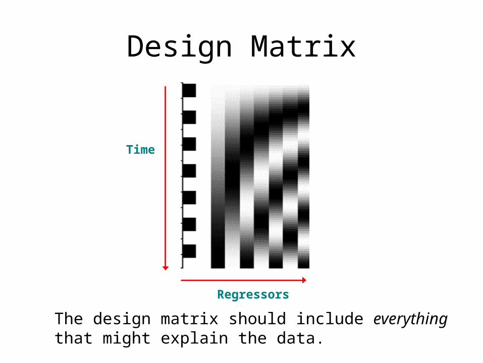
Design Matrix
The design matrix should include everythingthat might explain the data.
Regressors
Time
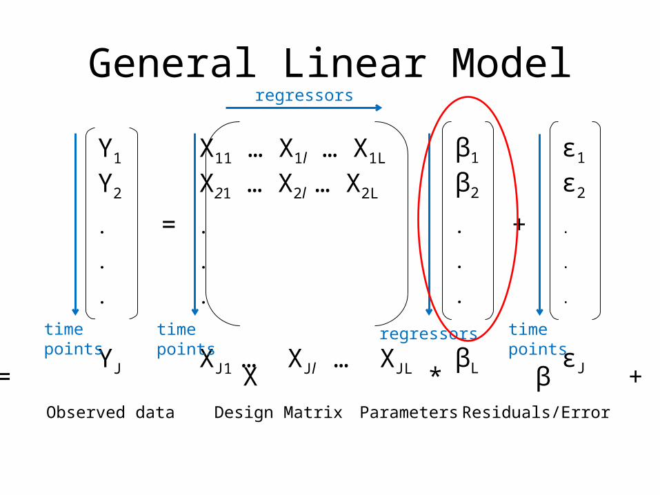
General Linear Model
Y1
Y2
.
.
.
YJ
=
X11 … X1l … X1L
X21 … X2l … X2L
.
.
.
XJ1 … XJl … XJL
β1
β2
.
.
.
βL
+
ε1
ε2
.
.
.
εJY = X * β + ε
Observed data Design Matrix Parameters Residuals/Error
timepoints
timepoints
regressors
regressors timepoints

Error
• Independent and identically distributed
),0(~ 2 Niid

Ordinary Least Squares
0 2 4 6 8 10 12 14 160
5
10
15
20
25
30
35
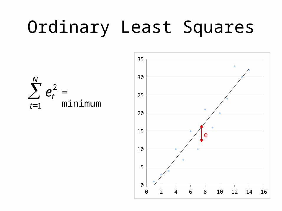
Residual sum of square:
The sum of the square difference between actual value and fitted value. e
Ordinary Least Squares
0 2 4 6 8 10 12 14 160
5
10
15
20
25
30
35
e
å=
N
tte
1
2 = minimum

Ordinary Least Squares
x1β1
x2β2
ye
Xβ
Y = Xβ+ee = Y-Xβ
XTe=0=> XT(Y-Xβ)=0=> XTY-XTXβ=0=> XTXβ=XTY=> β=(XTX)-1XTY
fMRI
12
Y = X * β + ε Observed data Design Matrix Parameters Residuals/Error

Problems with the model

The Convolution Model
=
Impulses HRF Expected BOLD
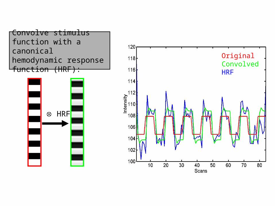
Convolve stimulus function with a canonical hemodynamic response function (HRF):
HRF
OriginalConvolvedHRF
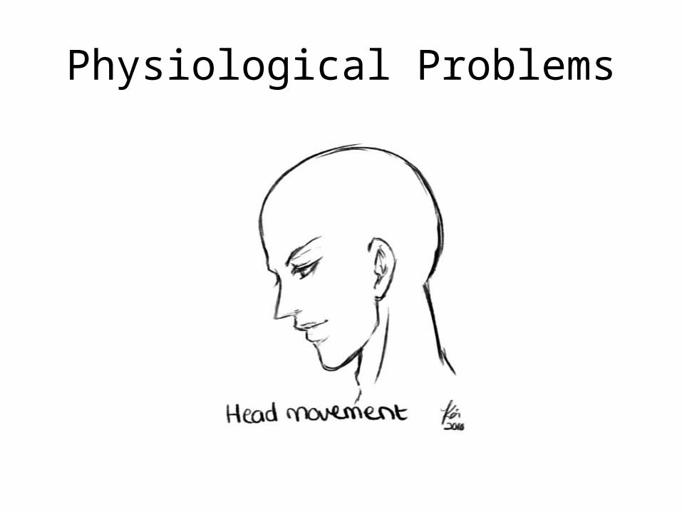
Physiological Problems


Noise
Low-frequency noise
Solution: High pass filtering
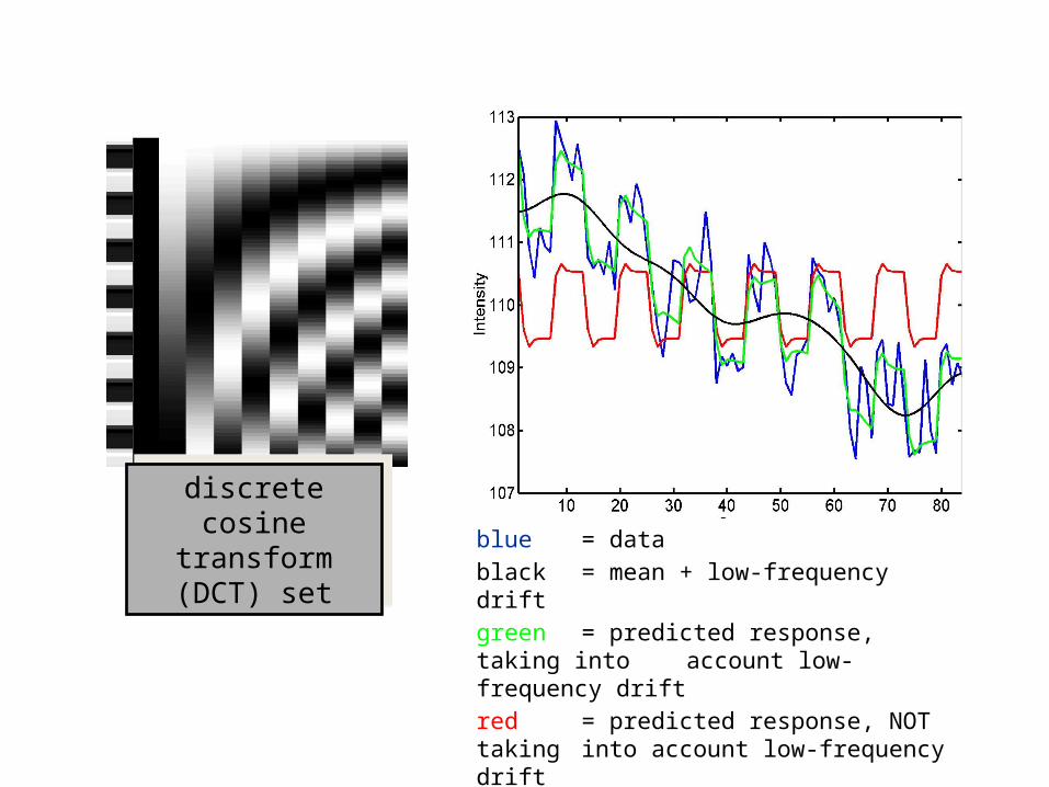
blue = data
black = mean + low-frequency drift
green = predicted response, taking into account low-frequency drift
red = predicted response, NOT taking into account low-frequency drift
discrete cosine transform (DCT) set
discrete cosine transform (DCT) set

Assumptions of GLM using OLS
AllAbout
Error
),0(~ 2INe

Unbiasedness
Expected value of beta =
beta

Normality

Sphericity

Homoscedasticity

not

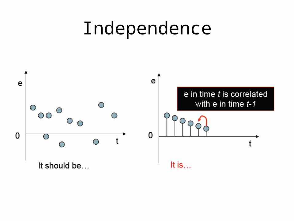
Independence
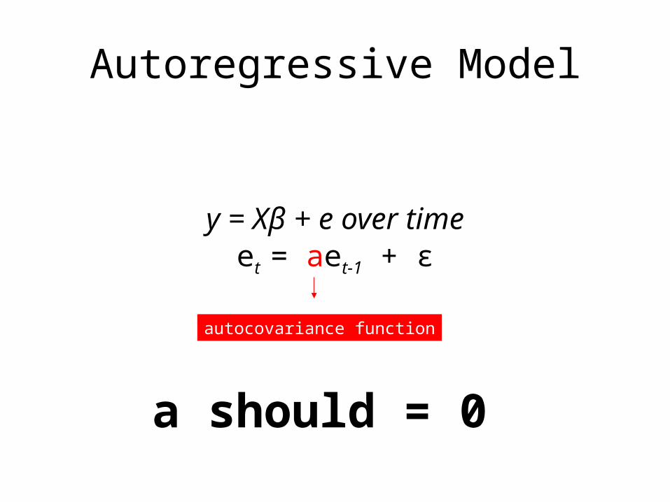
Autoregressive Model
y = Xβ + e over timeet = aet-1 + ε
autocovariance function
a should = 0

Thanks to…
• Dr. Guillaume Flandin
References• http://www.fil.ion.ucl.ac.uk/spm/doc/books/hbf2/pdfs/Ch7.pdf• http://www.fil.ion.ucl.ac.uk/spm/course/slides10-vancouver/02_General_
Linear_Model.pdf• Previous MfD presentations