GAUSSIAN MEASURE vs LEBESGUE MEASURE AND ELEMENTS …web.iku.edu.tr/ias/documents/karakoysem.pdf ·...
39
GAUSSIAN MEASURE vs LEBESGUE MEASURE AND ELEMENTS OF MALLIAVIN CALCULUS λ : Lebesgue measure has the following properties : 1. For every non-empty open set U,λ(U ) > 0 ; 2. For every bounded Borel set K,λ(K ) < ∞; 3. For every Borel set B,λ(B + x)= λ(B); (translational invariance) , further 4. λ has inner, outer regularity . In fact 1), 2) 3) nearly characterize the Lebesgue measure (modulo a multiplicative constant). Does the Lebesgue measure make sense in infinite dimensions ? The answer is negative. To convince ourselves : 1
Transcript of GAUSSIAN MEASURE vs LEBESGUE MEASURE AND ELEMENTS …web.iku.edu.tr/ias/documents/karakoysem.pdf ·...
GAUSSIAN MEASURE vs LEBESGUE
MEASURE AND
ELEMENTS OF MALLIAVIN CALCULUS
λ : Lebesgue measure has the following properties :
1. For every non-empty open set U , λ(U) > 0 ;
2. For every bounded Borel set K , λ(K) <∞;
3. For every Borel set B , λ(B + x) = λ(B) ; (translational
invariance) , further
4. λ has inner, outer regularity .
In fact 1), 2) 3) nearly characterize the Lebesgue measure
(modulo a multiplicative constant). Does the Lebesgue measure
make sense in infinite dimensions ? The answer is negative. To
convince ourselves :
1
H : a separable Hilbert space with an orthonormal basis h1, h2, · · · , ν
: a Borel measure in H
Let B 1
2
(hn) be the open ball of radius half, centered at hn ,
similarly B = B2(0) ;
By 1), 2) and 3) 0 < ν(B 1
2
(h1)) = ν(B 1
2
(h2) = · · · · · · < ∞ ,
but
ν(B2(0)) ≥∑
n ν(B 1
2
(hn) = ∞ violates 2).
Gaussian measure in Rn is absolutely continuous with respect
to the Lebesgue measure in n dimensions with Radon-Nikodym
derivative (density)
Φ(x) =1
(2π)n/2√DetS
e−1
2(S−1(x−m),x−m)), x ∈ Rn
m : Mean vector , S : Covariance matrix (symmetric, positive
definite) ;
2
Standard Gaussian Measure : m = 0 , S = I −→
Φ(x) = 1(2π)n/2
e−‖x‖2
2 x ∈ Rn .
Another way of outlook at the density : random element in Rn
∃(Ω,F , P ) and a measurable mapping X : Ω → Rn induces a
prob. measure µ in Rn : (assumed to be absolutely continuous)
µ(B) = P (X−1(B)) =∫
B Φ(x)dx ; B ∈ Bn
Standard Gaussian measure in finite dimensions is rotationally
invariant :∫
A−1B Φ(x)dx =∫
B Φ(x)dx .
Gauss distribution in finite dimensions can also be given by its
Fourier transformation (characteristic functional) :
χ(f) =
∫
Rn
ei(f,x)Φ(x)dx, f ∈ Rn ,
χ(f) = ei(f,m)− 1
2(Sf,f) f ∈ R
n
For n = 1 , f = t , χ(t) = eimt−σ2t2
2 .
3
The char. fn of random variable (f, x), f, x ∈ Rn) :
χf(t) =∫
Rn eit(f,x)Φ(x)dx = χ(tf) = eit(f,m)− t2
2(Sf,f) , (∗)
thus Gauss (in one dimension), converse is also true, i.e. if (f, .)
is one dimensional Gauss for all f ∈ Rn, then the measure in
Rn is Gaussian (put t = 1 in (*) ). Hence
µ ∈ Rn is Gaussian ⇐⇒ (f, .) has one dmnl Gaussian dist
forall f ∈ Rn
Take this point of view to define Gaussian measure in infinite
dimensions :
-A measure on a Hilbert space H is Gaussian ⇐⇒ (x, .) is a
Gaussian r.v. ∀x ∈ H
-A measure on a Banach space X is Gaussian ⇐⇒ (f, .) is a
Gaussian r.v. ∀f ∈ X∗ .
4
Two Problems : A) How to characterize the Fourier trans-
form of a finite measure
B) How to characterize the Fourier transform of Gaussian mea-
sures ?
Theorem 1 (Bochner) In Rn a functional µ(f) is the
Fourier transform of a finite measure ⇐⇒ µ(0) = µ(Rn),
continuous and positive definite.
For infinite dimensional Hilbert spaces these are not sufficient ,
e.g. e−1
2‖x‖2 satisfy the conditions but not the Fourier trans-
form µ(x) =∫
H ei(x,y)dµ(y) x ∈ H of any finite Borel
measure on the Hilbert space . (Otherwise for an orthonormal basis
hn ,∫
Hei(hn,y)dµ(y) = e−
1
2 which is not compatible with (hn, y) → 0
as∑
n(y, hn)2 = ‖y‖2 <∞) .
Definite answer
Theorem 2 (Minlos - Sazonov). Let φ be a positive-
definite fnl on H , then the following are equivalent :
5
i) φ is the Fourier transform of a finite Borel measure on H ,
ii) ∀ǫ > 0 , ∃ a symmetric, trace class operator Sǫ , such that
(Sǫx, x) < 1 =⇒ Re(φ(0)− φ(x) < ǫ ,
iii) ∃ a symmetric, trace class operator S on H , such that
φ is continuous (or continuous at x = 0) w.t. the norm
‖ . ‖∗ defined by ‖x‖∗ .= (Sx, x)1/2 = ‖S1/2x‖.
If µ is a Borel prob. measure then the mean vector is a vector
m ∈ H satisfying
(m, x) =∫
H(x, z)dµ(z) .
If∫
H ‖x‖ dµ(x) <∞ , it always exists. On the other hand :
6
Lemma 1. If µ is a finite Borel measure, then
∫
H ‖x‖2 dµ(x) <∞ ⇐⇒ ∃ a positive, symmetric, linear, trace
class operator , called S-Operator, such that ∀x, y ∈ H
(Sx, y) =∫
H(x, z)(y, z)dµ(z) .
If further µ is a probability measure then B, Bx.= Sx −
(m, x)x satisfies
(Bx, y) =∫
H(z − m, x)(z − m, y)dµ(z) is the covariance
operator.
A Gaussian probability on H (i.e. all (x, .) are one-dimensional
Gaussian r.v.s ) always satisfies the above conditions, thus m
and B always exists.
7
In fact ;
Theorem 3. A Borel probability measure µ on H is Gaussian
⇐⇒ Its Fourier transform can be expressed as
µ(x) = exp i(m, x)− 1
2(Bx, x) , ∀m, x ∈ H .
In a Banach space X the definition of the mean vector is the
same. If we use the random element outlook, the mean vector
m ∈ X can be given by a Pettis integral
< m, f >.=∫
Ω < f, x(ω) > dP (ω) , ∀f ∈ X∗ . (†)
Thus a necessary condition for the existence of m ∈ X is that
< f, x(.) >∈ L1(Ω,F , P ) ∀f ∈ X∗ . If the necessary condi-
tion is satisfied then the r.h.s. of (†) defines a linear , continuous
function of f , i.e. an element of X∗∗.
8
Hence if m exists m ∈ X ∩ X∗∗, (X → X∗∗) . Therefore for
the reflexive spaces , the necessary condition is also sufficient.
In the non-reflexive case there are extra sufficient conditions.
Leaving them out we know that for Gaussian distribution m
always exists.
The covariance operator in X is defined through an S-operator
S : X∗ → X∗∗ , i.e.
<< Sf, g >>=∫
X < f, z >< g, z > dµ(z), f, g ∈ X∗ and
Bf = Sf− < m, f > m (Covariance operator).
Operator S has properties akin to operators S : H → H e.g.
:
i) Symmetry : << Sf, g >>=<< Sg, f >> ;
ii) Positivity : << Sf, f >>≥ 0, ∀f ∈ X∗ .
9
The existence of the covariance operator in a Banach space is
characterized in terms of the nuclearity of S or B but a mod-
ified definition of nuclearity is needed in Banach spaces. Let
H(X) : all symmetric, non-negative , bounded linear mappings
X∗ → X∗∗ ;
H1(X) : the class of covariance operators of distributions on
X ;
H2(X) : the classs of covariance operators of all Gaussian dis-
tributions on X. (H2(X) ⊂ H1(X) ⊂ H(X))
If X is separable and reflexive then H1(X) = H(X) . Under the
same conditions,for S ∈ H(X) , nuclearity in the first sense is
sufficient and the nuclearity in the second sense is necessary for
S to be in H2 , (For nuclearity of different senses c.f. [Vakha-
nia]).
10
If we consider for simplicity m = 0 ,
χ(f ;µ) = exp −12 << Sf, f >> ∀f ∈ X∗ (
√)
is the Fourier transform of some Gaussian measure in X
⇐⇒ S ∈ H2 .
Standard Gaussian Cylinder Measures
The quasi-invariance property which is so important in the dif-
ferential analysis in infinite dimensions is possessed by the stan-
dard Gaussian measure where m = 0 and S = I. However
S = I does not make sense in (√) as an operator X∗ → X∗∗ ,
and in the Hilbert case I is not nuclear (or trace class ) and
χ(f) = e−1
2‖f‖2 obtained by B = I can not be the charac-
teristic functional of a standard type Gaussian distribution in
X. Therefore an approach via finite dimensional subspaces is
essential.
11
Let F(X∗) : be the class of all finite dimensional subspaces of
X∗ ;
For any K ∈ F(X∗) call
D = x ∈ X : (< x, y1 >,< x, y2 >, · · · , < x, yn >) ∈ E
a cylinder set based on K if E ∈ Bn, y1, · · · , yn ∈ K.
Let ℜ(X) =⋃
K∈F(X∗) C(K) , where C(K) is the σ-algebra
generated by cylinder sets with base K.
ℜ(X) is only an algebra , but for a separable Banach space
X, σ(ℜ(X)) = BX (the Borel σ-alg. in X).
A non-negative set fct µ on ℜ(X) is called a ”cylinder prob-
ability measure” on X , if µ(X) = 1 and a measure when
restricted to any C(K) for K ∈ F(X∗) . A cylinder probability
measure is necessarily compatible.
A real (complex)-valued fct on X is a cylinder fct if it is mea-
surable w.t. C(K) for some K.
µ(f) =∫
X ei<x,f>dµ(x) , f ∈ X∗ : the characteristic fnl of
the cylinder measure µ .
12
Question : What kind of cylinder measures can be extended
to BX ?
Answer in a Special Case (Important for Malliavin calculus)
X is the completion of some Hilbert space H w.t. a weaker
norm and the cylinder measure on X is lifted from that on H.
Definition 1. (Gross) Let (H, | . |) be a Hilbert space , µ
a cylindrical measure on H, ‖ . ‖ another norm on H weaker
than | . | If for any ǫ > 0 ∃ πǫ ∈ P ( the set of all finite
dimensional orthogonal projections on H ), such that for any
π ∈ P (π ⊥ πǫ) one has µx ∈ H : ‖πx‖ > ǫ < ǫ then ‖ . ‖
is said to be a measurable norm with respect to µ.
(Cylinder measures can also be defined on H : since
X∗ → H∗ ≃ H we have F(X∗) ⊂ F(H) )
If µ is a cylinder measure on H and µ(x) = e−1
2|x|2 , x ∈ H
then µ is called a ”standard Gaussian cylinder measure” on H.
13
Theorem 4.(Gross) Suppose the triplet (X,H, µ) is as above.
If µ is a Gaussian cylinder measure on H and ‖ . ‖ is a µ-
measurable norm, then the lifting µ∗ of µ to X can be ex-
tended to a Borel measure on X , called Standard Gaussian
measure on X . µ∗(C).= µ(C ∩H) , C ∈ R(X)) .
(X,H, µ) is called an abstract Wiener space
Conversely let X be a separable Banach space and let µ be
a zero mean Gaussian measure on X , i.e. for any α ∈ X∗
and ω ∈ X , < α, ω > is a one-dimensional zero mean Gauss
random variable (or for any n and αi ∈ X∗ < αi, ω > , i =
1, 2, · · ·n is a zero mean Gaussian random vector) .Then there
exists a dense Hilbert sub-space H ⊂ X such that (X,H, µ)
is an abstract Wiener space.
H is called the Cameron-Martin space.
14
Classical Wiener space is an example of an abstract Wiener
space :
Banach space X : C0[0, 1] with the sup norm,
For ω ∈ C0[0, 1] , t ∈ [0, 1] coordinate functional on C0[0, 1]
is Wt(ω) = ω(t) .
N. Wiener : There exists a unique probability µ on BC0such
that the map (t, ω) −→ Wt(ω) is a Wiener process (Brownian
motion).
H : absolutely continuous functions in C0[0, 1] with square
integrable derivatives.
Then h ∈ H ⇒ h =∫ t
0 h(s)ds , h ∈ L2[0, 1] .
‖h‖C0= sup0≤t≤1 |
∫ t
0 h(s)ds| ≤ sup0≤t≤1
(
t∫ t
0 |h(s)ds)
1
2 ≤(
∫ t
0 |h(s)|2ds)
1
2
= (∫ t
0 |h|2)1
2
.= |h|H . (defn of norm in H).
15
With this norm h → h is a continuous , linear injection from
H into C0, such that its range is dense in C0 . ‖ . ‖ is weaker
than | . | when restricted to H.
If (X,H, µ) is an abstract Wiener space , considering that the
cylindrical measure is on H, we want to construct a process
< h, ω > , h ∈ H,ω ∈ X .
But since X∗ ⊂ H , h may not be in X∗ . However X∗ is
densely imbedded in H. Indicate the injection X∗ → H∗ ≃
H by ˆ( . ), α ∈ X∗ → α ∈ H . Given h ∈ H there exists
αn ∈ X∗ s.t. αn −→ h in H. For ω ∈ X the Gaussian
sequence < αn, ω > is Cauchy in Lp, denote the limit by
Wh(ω) , (δh(ω) in some sources ), which is N(0 , |h|2H) and
also E(WhWg) = (h, g)H , h, g ∈ H .
Thus we have another model which is called Gaussian prob-
ability space by Malliavin. Namely :
16
(Ω,F , µ) : a complete probability space, H : a real, separable
Hilbert space, Wh, h ∈ H is a family of zero mean Gaussian
r.v.’s with E[WhWg] = (h, g)H .
(Ω,F , µ;H) A Gaussian probability space. The classical and
abstract Wiener spaces are examples of Gaussian probability
spaces. A third example is the White noise space : H =
L2(R) ; S(R), S∗(R) : Schwartz spaces of rapidly decreasing
C∞ functions and tempered distributions respectively. ( S(R) ⊂
L2(R) ⊂ S∗(R) is called a Gelfand Triplet). Then by
the Minlos theorem there exists a unique Gaussian measure µ
on BS∗(R) such that ∀ξ ∈ S(R) :∫
S∗(R) ei<ω,ξ>dµ(ω) =
e−1
2‖ξ‖2H ; < ω, ξ > is the canonical bilinear form on S∗(R) ×
S(R) . Then Wξ(ω) =< ω, ξ > ξ → Wξ can be ex-
tended to a linear isometry L2(R) −→ L2(S∗(R),F , µ) , thus
(S∗(R),F , µ;L2(R)) is a Gaussian probability space.
17
In an abstract Wiener space or a Gaussian probability space ,
Wh(ω), h ∈ H is like a stochastic process with the index set
H .
Some Elements of the Malliavin Calculus
In an abstract Wiener space (or a Gaussian probability space)
F : X → R(C) is called a Wiener functional.
Some examples ; Ito stochastic integrals, solutions of stochastic
differential equations. As they are in fact equivalence classes ,
may not be differentiable in the Frechet sense, even not contin-
uous. Paul Malliavin , using the quasi-invariance of the Gaus-
sian measure, initiated a kind of weak differential calculus, so
that such functionals became smooth in his sense . The quasi-
invariance is translational invariance of the Gaussian measure in
the directions of the Cameron-Martin space H.
18
The new kind of differentiation was obtained by perturbing the
Wiener paths in the directions of vectors in H, thus taking the
name of ”stochastic calculus of variation” or as popularly known
the Malliavin calculus.
If F : X −→ R an attempt to define the derivative by
lim‖∆ω‖→0F (ω +∆ω)− F (ω)
‖∆ω‖ will fail since the quotient is not
even well-defined as a random variable, (equivalence classes).
This is remedied by the Cameron-Martin Formula (Theorem):
E[F (ω + h)] = E[F (ω)eWh− 1
2|h|2H ]
If in the above quotient the perturbation ∆ω = h is taken in
the Camerion Martin space, (i.e. h ∈ H) then the limit will be
well-defined .
Take two functionals in the same equivalence class :
19
F = G µ−a.s. =⇒ µω|F (ω+h) 6= G(ω+h) = Eµ
Iω|F (ω+h) 6=G(ω+h)
= (Cameron-Martin thm.) Eµ
Iω|F (ω) 6=G(ω)eWh− 1
2|h|2H
= 0 .
This allows to define weak differential (Sobolev derivative) start-
ing from cylindrical functionals.
Let (X,H, µ) be an abstract Wiener space.
F (ω) = f (Wh1(ω), · · · · · · ,Whn
(ω)) , ω ∈ X, f ∈ S(Rn)
is called a smooth cylindrical functional, its class is de-
noted by SM . Similarly depending on f being a polynomial
or Lp function we have a functional in P or in Lp(µ) . The
following inclusions hold
P ⊂ SM ⊂ Lp
and P is dense in Lp . Noticing that Whj(ω+λh) = Whj
(ω)+
λ(hj, h)H we have the following definition of the weak direc-
tional derivative (Sobolev derivative) :
20
DhF (ω) =d
dλF (ω+λh)|λ=0 =
n∑
i=1
∂f
∂xj(Wh1
(ω), · · · ,Whn(ω))(hj, h)H ; h ∈ H.
For fixed ω , h → Dh(ω) is linear and continuous , hence it
determines (by the Riesz representation thm) an element of
H∗ ≃ H that we denote by DF (the gradient operator) and
(DF, h)H = DhF and also E[(Df, h)] = E[F (Wh))] .
21
Also F (ω) −→ DF (ω) is a linear operator from the cylindri-
cal functionals into the space of H-valued Wiener functionals
Lp(µ;H) ,
(the norm being defined by ‖DF (ω)‖p =[∫
X |DF (ω)|pHdµ(ω)]
1
p ) .
Note. If G ∈ Lp(µ) and F = G (µ − a.s.) then by the
Cameron-Martin thm. G(ω + λh) = F (ω + λh) (µ − a.s.) ,
thus DF depends only on the equivalence class that F belongs
to.
We want to extend the above operator to a larger class of Wiener
functionals. In fact we have
Theorem 5. D is a closable operator from Lp(µ) into Lp(µ;H) .
22
Definition 2. Dp,1 is the set of equivalence classes of Wiener
functionals defined by :
F ∈ Dp,1 ⇔ ∃ a sequence of cylindrical fcts Fn converging to
F in Lp(µ) such that DFn , n ∈ N is Cauchy in Lp(µ;H).
In this case denote limn→∞DFn = DF .
(DF is independent of the choice of the sequence Fn) .
Dp,1 is a Banach space under the norm ‖F‖pp,1 = ‖F‖pLp(µ) +
‖DF‖pLp(µ;H) .
Generalization to E valued functionals (E is any separable Hilbert
space ):
DhF = (DF, h) takes the form :
ddλ [(F (ω + λh), e)E] |λ=0 = (DF (ω), h ⊗ e)H⊗E h ∈ H , e ∈
E .
DF ∈ Lp(µ;H ⊗ E) . Corresponding Sobolev space is denoted
by Dp,1(E) .
23
Higher order derivatives and Sobolev spaces are defined in an
inductive manner:
D2F = D(DF ) ∈ Lp(H⊗H⊗E) · · · · · · , DkF = D(Dk−1F ) ∈ Lp(H⊗(k)⊗E) .
where ⊗ denotes the (completed) Hilbert tensor product. Sim-
ilarly F ∈ Dp,k if Dk−1F ∈ Dp,1(H⊗(k−1)⊗E) and the norms
‖F‖p,k =(
‖F‖pp +k∑
j=1
‖DjF‖pp
)1/p
.
Since the gradient DF is an H-valued functional, H may be
considered as tangent space. Hence H-valued functionals are
vector fields and the adjoint operator δ is the divergence of
vector fields.
24
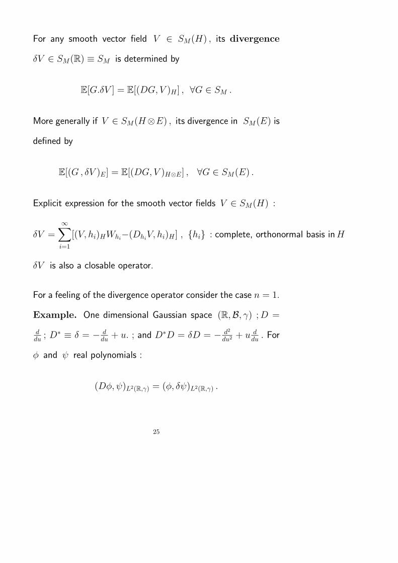
For any smooth vector field V ∈ SM(H) , its divergence
δV ∈ SM(R) ≡ SM is determined by
E[G.δV ] = E[(DG, V )H ] , ∀G ∈ SM .
More generally if V ∈ SM(H⊗E) , its divergence in SM(E) is
defined by
E[(G , δV )E] = E[(DG, V )H⊗E] , ∀G ∈ SM(E) .
Explicit expression for the smooth vector fields V ∈ SM(H) :
δV =∞∑
i=1
[(V, hi)HWhi−(Dhi
V, hi)H ] , hi : complete, orthonormal basis inH
δV is also a closable operator.
For a feeling of the divergence operator consider the case n = 1.
Example. One dimensional Gaussian space (R,B, γ) ;D =
ddu ; D
∗ ≡ δ = − ddu + u. ; and D∗D = δD = − d2
du2 + u ddu . For
φ and ψ real polynomials :
(Dφ, ψ)L2(R,γ) = (φ, δψ)L2(R,γ) .
25
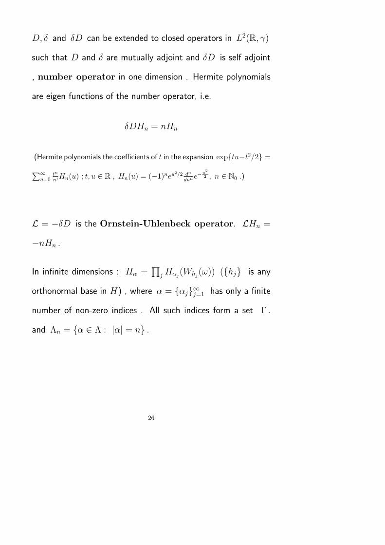
D, δ and δD can be extended to closed operators in L2(R, γ)
such that D and δ are mutually adjoint and δD is self adjoint
, number operator in one dimension . Hermite polynomials
are eigen functions of the number operator, i.e.
δDHn = nHn
(Hermite polynomials the coefficients of t in the expansion exptu−t2/2 =
∑
∞
n=0tn
n!Hn(u) ; t, u ∈ R , Hn(u) = (−1)neu
2/2 dn
dune−
u2
2 , n ∈ N0 .)
L = −δD is the Ornstein-Uhlenbeck operator. LHn =
−nHn .
In infinite dimensions : Hα =∏
jHαj(Whj
(ω)) (hj is any
orthonormal base in H) , where α = αj∞j=1 has only a finite
number of non-zero indices . All such indices form a set Γ .
and Λn = α ∈ Λ : |α| = n .
26
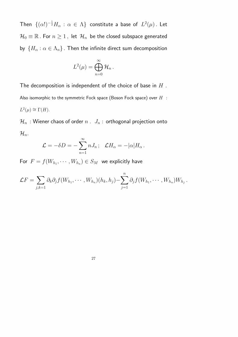
Then (α!)− 1
2Hα : α ∈ Λ constitute a base of L2(µ) . Let
H0 ≡ R . For n ≥ 1 , let Hn be the closed subspace generated
by Hα : α ∈ Λn . Then the infinite direct sum decomposition
L2(µ) =∞⊕
n=0
Hn .
The decomposition is independent of the choice of base in H .
Also isomorphic to the symmetric Fock space (Boson Fock space) over H :
L2(µ) ∼= Γ(H).
Hn : Wiener chaos of order n . Jn : orthogonal projection onto
Hn.
L = −δD = −∞∑
n=1
nJn ; LHα = −|α|Hα .
For F = f(Wh1, · · · ,Whn
) ∈ SM we explicitly have
LF =∑
j,k=1
∂k∂jf(Wh1, · · · ,Whn
)(hk, hj)−n∑
j=1
∂jf(Wh1, · · · ,Whn
)Whj.
27
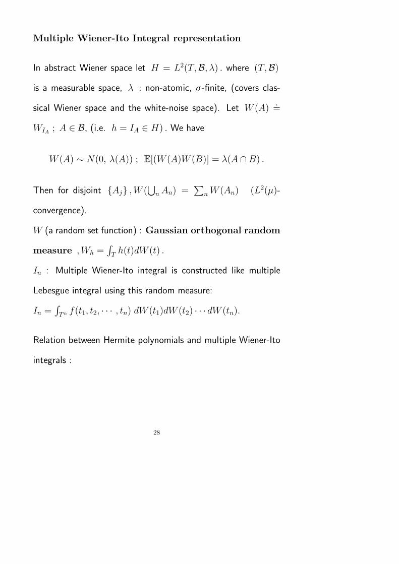
Multiple Wiener-Ito Integral representation
In abstract Wiener space let H = L2(T,B, λ) . where (T,B)
is a measurable space, λ : non-atomic, σ-finite, (covers clas-
sical Wiener space and the white-noise space). Let W (A).=
WIA ; A ∈ B, (i.e. h = IA ∈ H) . We have
W (A) ∼ N(0, λ(A)) ; E[(W (A)W (B)] = λ(A ∩B) .
Then for disjoint Aj ,W (⋃
nAn) =∑
nW (An) (L2(µ)-
convergence).
W (a random set function) : Gaussian orthogonal random
measure ,Wh =∫
T h(t)dW (t) .
In : Multiple Wiener-Ito integral is constructed like multiple
Lebesgue integral using this random measure:
In =∫
Tn f(t1, t2, · · · , tn) dW (t1)dW (t2) · · · dW (tn).
Relation between Hermite polynomials and multiple Wiener-Ito
integrals :
28
Hn(Wh) = In(h⊗n) . For n = 1 , H1(u) = u then it reduces to
∫
T h(t)dW (t) = H1(Wh) = Wh .
More generally if hjj∈N is a base of H we have Hα =
I|α|(hα) , ∀α ∈ Λ and hα ≡ ˆ⊗jh
⊗αj
j .
Also F ∈ L2(µ) has a unique decomposition F =∑∞
n=0 In(fn)
where fn ∈ H⊗n and ‖F‖2 = [E(|F |)2 +∑∞n=0 n!‖fn‖2
(‖fn‖ stands for the norm in L2(T n,Bn, λn)) .
Another interpretation of the Ornstein-Uhlenbeck
Operator L = −δD
Ornstein-Uhlenbeck process satisfies the stochastic d.e.
dXt = −Xtdt+√2 dBt , X0 = x ∈ R
n (Bt : Brownian motion)
has the solution Xt = e−tx +√2∫ t
0 e−(t−s)dBs t ∈ R+ . Xt
is a Gaussian process Xt ∼ N(e−tx, 1 − e−2t) . Define the
Ornstein-Uhlenbeck semi-group Tt which is a contraction (even
e hypercontractive) semi-group.
29
(Ttφ)(x).= E[φ(Xt)] =
∫
X
φ(e−tx+√
1− e−2ty) dµ(y) ; φ ∈ SM
(µ : standard normal distribution) . Semi-group property follows
from the Markov property of diffusion processes and it turns out
that the infinitesimal generator of this semi-group is L . There-
fore Tt = etL =∑∞
n=0tnLn
n!. Using L0 ≡ I =
∑
n Jn, L =
∑
n nJn, L2 = (∑
n−nJn)(∑
m−mJm) =∑
n n2Jn , (the or-
thogonality of chaos projections) and by induction Lm =∑
n(−1)mnmJn
yielding for the representation of the O-U semigroup Tt =
∑∞n=0 e
−ntJn .
As each Wiener chaos belongs to the eigen-space of L , we can
define non-integer powers, e.g., (I−L)a = I−aL+ a(a−1)2
L2−· · · =∑
Jn + a∑
nJn + (a(a−1)2
n2Jn + · · · =∑
(1 + an + a(a−1)2
n2 + · · · )Jn =
∑
n(1 + n)aJn ;
30
In particular for p > 1 , a = −12 , the completion of polynomial
cylindrical functionals with respect to the norm
‖F‖∼p,k.= ‖(I − L)k
2F‖Lp is dense in Lp and denoted by D∼p,k .
Now the important Meyer inequalities relating Sobolev and Lp
norms
∀p > 1, ∀k ∈ N ∃cp,k , cp,k , such that ∀F ∈ P(E) :
cp,k‖(I − L)k2F‖Lp(µ;E) ≤ ‖F‖p,k ≤ cp,k‖(I − L)k
2F‖Lp(µ;E) .
By these inequalities for k ∈ N , ‖ . ‖ ∼ ‖ . ‖∼ , then we omit
∼ sign, but whenever k is non-integer we should know that
Dp,k ≡ D∼p,k . Using Meyer inequalities we show (for E valued
functionals) :
31
i) Dp,k(E) has Dq,−k(E) its continuous dual , 1/p+1/q = 1 ,
ii) D has a continuous extension from Dp,k(E) into Dp,k−1(E⊗
H) for any p > 1 ,
iii) δ has a continuous extension from Dp,k(E⊗H) into Dp,k−1(E)
for any p > 1 .
Generalized Functions
Similar to the test functions-Schwartz distributions dual-pair
(D,D∗) we have :
D∞(E) =
⋂
k>0
⋂
1<p<∞Dp,k(E) , D
−∞(E) =⋃
k>0
⋃
1<p<∞Dp,−k(E) .
D∞ is equipped with the projective limit topology and D
−∞
is equipped with the inductive limit topology ; the latter is the
Meyer-Watanabe distributions.
As an application Donsker’s Delta Function is δx(W (t)) ∈
D−∞ .
32
Using Meyer inequalities one can show that :
• D uniquely extends to a continuous operator D∞(E) −→
D∞(E ⊗H) ,
• D uniquely extends to an operator D−∞(E) −→ D−∞(E⊗
H) ,
• Similar extensions for δ = D∗ , e.g. δ : D−∞(E ⊗H) −→
D−∞(E) ,
• L extends uniquely to an operator D−∞(E) −→ D
−∞(E)
such that ∀p ∈ (1,∞) , k ∈ R
L : Dp,k+2(E) −→ Dp,k(E) is continuous, in particular L : D∞(E) → D∞(E)
is continuous.
33
Densities of Non-degenerate Functionals
One of the main concerns of the Malliavin calculus is the investi-
gation of existence, regularity (smoothness) and other properties
of the Wiener (Brownian) functionals.
Let F be an Rm-valued functional (i.e. an m-dimensional ran-
dom vector). µ F−1 defines a probability measure on Bm .
Under which conditions it is absolutely continuous with respect
to the Lebesgue meaure λm ?
Malliavin Covariance Matrix
Let F = (F1, F2, · · · , Fm) ∈ D1,1(Rm) and σij
.= (DFi, DFj)H ;
1 ≤ i, j ≤ m.
Malliavin Matrix : Σ(ω) = 〈σij(ω)〉 .
If DetΣ(ω) > 0 a.s. and satisfies [DetΣ(ω)]−1 ∈ L∞− ≡⋂
1<p<∞ Lp(µ) , then we say F is non-degenerate in the sense
of Malliavin. The following is a key lemma of harmonic analysis:
34
Lemma 2. Let ν be a σ-finite measure on Bm . If for j =
1, 2, · · · ,m ∃cj such that ∀φ ∈ C∞0 (Rm) :
|∫
Rm
∂jφ(x)dν(x)| ≤ cj‖φ‖∞
then ν ≺≺ λm .Whenm > 1 , ν has density ρ ∈ Lm∗
(Rm) , m∗ =
mm− 1 .
Note : Clear for m = 1 : take φ the cumulative D.F. of the uniform
U([a, b]) r.v. It is not in C∞
0 . But ∃φn ∈ C∞
0 such that φn → φ , φ′
n →
φ′ , φ′ = 1b−a
, ‖φ‖∞ = 1 . Then the condition yields ν([a, b]) ≤
c1(b− a) = c1λ([a, b]) implying absolute continuity .
Lemma 2 is utilized to prove
Theorem 6. Let F = (F1, F2, · · · , Fm) ∈ D∞2 (Rm) ≡
⋂
1<p<∞Dp,2(Rm)
be non-degenerate. Then ∃Φj ∈ L∞−(µ) (j = 1, · · · ,m) such
that ∀φ ∈ C∞0 (Rm) , E[∂jφF ] = E[Φj(φF )] which implies
that F has a density ρ . In case m > 1 , ρ ∈ Lm∗
. If only the
existence of density is sought , the condition can be consider-
ably weakened : For p > 1 , F ∈ Dp,1(Rm) , if the Malliavin
covariance matrix is invertible, then F has a density.
35
Smoothness of Densities
The density of F can be formally expressed as E[δx F ] , (δx :
Dirac function with singularity at x ).
: (To see this heuristically consider a delta sequence δn,x → δx, then
∫
Ωδn,x(F (ω))dµ(ω) =
∫
Rmδn,x(y)p(y)dy → p(x) .)
However following Watanabe we should give a rigorous meaning
to the composition of a Schwartz distribution with a functional.
If φ ∈ S(Rm) and F ∈ D∞(Rm) , then the composite func-
tional φ F ∈ D∞ . For fixed F , φ → φ F is a linear map
S(Rm) → D∞ . Watanabe’s method is to extend it to a linear
and (in some sense) continuous map from S∗(Rm) → D−∞ .
He showed that in this way every Schwartz distribution T can be
lifted (pulled-back) to a generalized Wiener functional T F .
(Note that S ⊂ S∗ and because of Dp,k ⊂ Dp,−k we have
D∞ ⊂ D
−∞ ). Then δx F can be interpreted as a generalized
functional. Using Watanabe’s approach we prove
Theorem 7. If F ∈ D∞(Rm) is non-degenerate, then F has
density ρ which is infinitely differentiable.
36
Hypoellipticity and Hormander’s condition
Consider the second order partial differential operator
L =1
2
m∑
i,j=1
aij(.)∂i∂j +m∑
i=1
bi(.)∂i .
and the Cauchy problem for the heat equation :
∂tu(t, x) = Lu(t, x), t > 0, x ∈ Rm ;
u(0, x) = φ(x) .
It is known that if φ ∈ C2b (R
m) , then
uφ(t, x) ≡ E[φ(X(x, t, ω))]
is the solution of the Cauchy problem . X is the solution of the Ito
stochastic differential equation Xt = x+∫ t
0b(Xs)ds+
∫ t
0σ(Xs).dBs, t ≥ 0
where x ∈ Rm, b : Rm → R
m, σ : Rm → Rm ⊗ R
d .
If Xt is non-degenerate ([detΣ]−1 ∈ L∞−), then the transition
probability P (t, x, ω) = µ X(x, t, ω)−1 of diffusion process
X has C∞ density p(t, x, y) = E[δy(X(x, t, ω))] which is the
fundamental solution of the above Cauchy problem (the heat
kernel : uφ(t, x) =∫
Rd p(t, x, y)φ(y)dy).
37
From the theory of p.d.e. if matrix a(x) is uniformly positive
definite , i.e. ∃η > 0 such that a(.) ≥ ηI , then the conclusion
is true.
Hormander obtained a much weaker condition through the hy-
poellipticity of the differential operators, namely the Hormander
condition. To state Hormander’s theorem write L in form of vec-
tor fields :
Ak(.) ≡ σik(.)∂i , k = 1, · · · , d ,
A0(.) ≡ [bi(.) − 12
∑dk=1 σ
jk(.)∂jσ
ik(.)]∂i (with Einstein’s sum-
mation convention) , we have :
L = 12
∑dk=1A
2k + A0 .
Hormander’s Theorem for Hypoellipticity
If for every x ∈ Rm the Lie algebra generated by vector fields
Ak, [A0, Ak], k = 1, · · · , d) has dimension m (Hormander
condition) , then L is hypoelliptic , that is , for any open set
U ∈ Rm and any Schwartz distribution u ∈ D∗ if Lu|U ∈
C∞(U) , then u|U ∈ C∞(U)
If the Hormander’s condition holds, then (in the elliptic case)
the above smooth fundamental solution exists.
38
([ . , . ] is the Lie bracket : Given two C1 vector fields V and W on
Rm , [V,W ](x) = DV (x)W (x)−DW (x)V (x)) .
The key step in the probabilistic proof of the Hormander’ the-
orem is to show that under the Hormander’s condition the cor-
responding Malliavin covariance matrix is non-degenerate.
REFERENCES
Z.Huang & J.Yan : Introduction to Infinite Dimensional Stochastic Analysis
; Kluwer (2000)
H.H.Kuo : Gaussian Measures in Banach Spaces : Lecture Notes in Mathe-
matics no.463 , Springer(1975)
P.Malliavin : Stochastic Analysis ; Springer (1997)
D.Ocone : A Guide to the Stochastic Calculus of Variations ; Stochastic
Analysis and Related Topics, eds. Korezlioglu, Ustunel , Lecture Notes 1316,
pp. 1-97 . Springer (1987).
I.Shigekawa : Stochastic Analysis ; AMS Monographs ,vol.224 (2004)
A.S.Ustunel & M.Zakai : Transformation of Measure on Wiener Space :
Springer Monographs in Math. (2000)
N.N.Vakhania: Probability Distributions on Linear Spaces ; North Holland
(1981)
S.Watanabe : Lectures on Stochastic Differential Equations and Malliavin
Calculus ; Tata-Springer (1984).
39