Gaussian Distribution - Welcome to CEDAR€¦ · Machine Learning srihari 2 The Gaussian...

Machine Learning srihari

1

Gaussian Distribution

Sargur N. Srihari


2

The Gaussian Distribution

•  For single real-valued variable x

•  Parameters: –  Mean µ, variance σ 2,

•  Standard deviation σ •  Precision β =1/σ 2, E[x]=µ, Var[x]=σ 2

•  For D-dimensional vector x, multivariate Gaussian

�

N(x |µ,σ 2) = 1(2πσ 2)1/ 2

exp − 12σ 2 (x − µ)2

⎧ ⎨ ⎩

⎫ ⎬ ⎭

µ is a mean vector, Σ is a D x D covariance matrix, |Σ| is the determinant of Σ

Σ-1 is also referred to as the precision matrix

Carl Friedrich Gauss 1777-1855

N(x | µ,Σ) =

1(2π)D/2

1|Σ |1/2

exp −12(x−µ)TΣ−1(x−µ)

⎧⎨⎪⎪

⎩⎪⎪

⎫⎬⎪⎪

⎭⎪⎪

68% of data lies within σ of mean 95% within 2σ


Covariance Matrix

•  Gives a measure of the dispersion of the data •  It is a D x D matrix

– Element in position i,j is the covariance between the ith and jth variables.

•  Covariance between two variables xi and xj is defined as E[(xi-µi)(yi-µj)]

•  Can be positive or negative

–  If the variables are independent then the covariance is zero.

•  Then all matrix elements are zero except diagonal elements which represent the variances 3


4

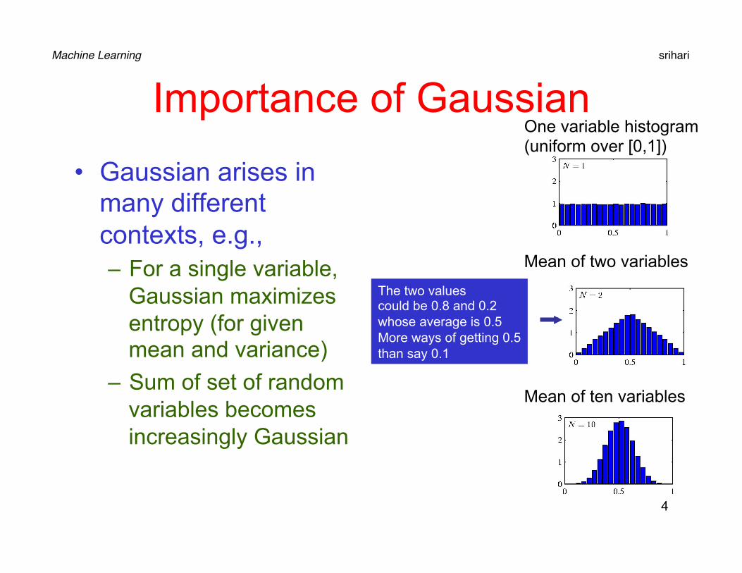
Importance of Gaussian

•  Gaussian arises in many different contexts, e.g., –  For a single variable,

Gaussian maximizes entropy (for given mean and variance)

–  Sum of set of random variables becomes increasingly Gaussian

One variable histogram (uniform over [0,1])

Mean of two variables

Mean of ten variables

The two values could be 0.8 and 0.2 whose average is 0.5 More ways of getting 0.5 than say 0.1


5

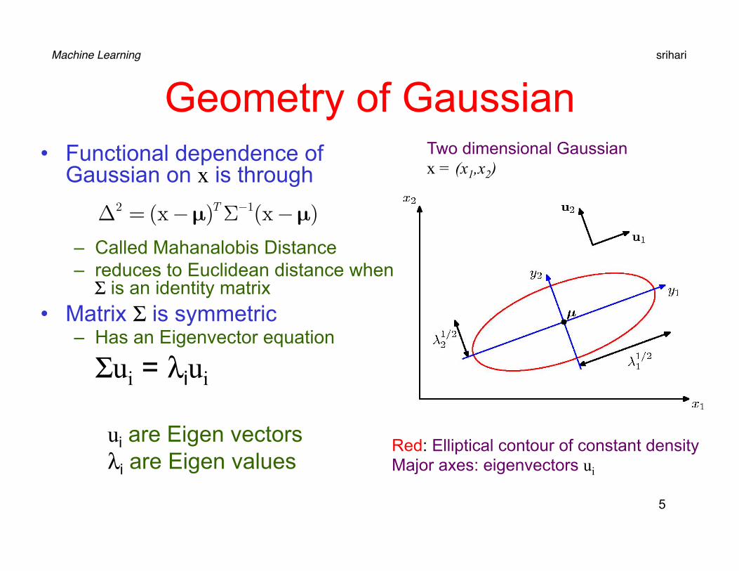
Geometry of Gaussian •  Functional dependence of

Gaussian on x is through

–  Called Mahanalobis Distance –  reduces to Euclidean distance when

Σ is an identity matrix •  Matrix Σ is symmetric

–  Has an Eigenvector equation

Σui = λiui

ui are Eigen vectors λi are Eigen values

Two dimensional Gaussian x = (x1,x2)

Red: Elliptical contour of constant density Major axes: eigenvectors ui

Δ2 = (x−µ)TΣ−1(x−µ)


6

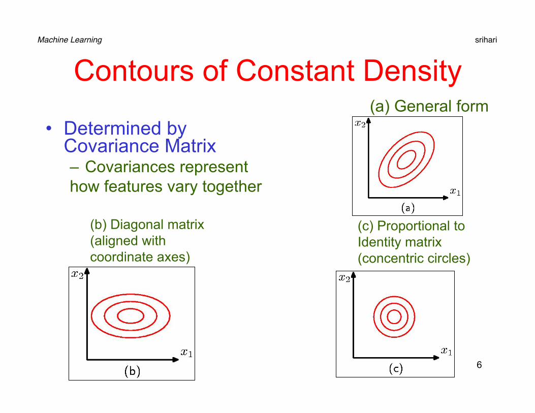
Contours of Constant Density

•  Determined by Covariance Matrix –  Covariances represent how features vary together

(a) General form

(b) Diagonal matrix (aligned with coordinate axes)

(c) Proportional to Identity matrix (concentric circles)


7

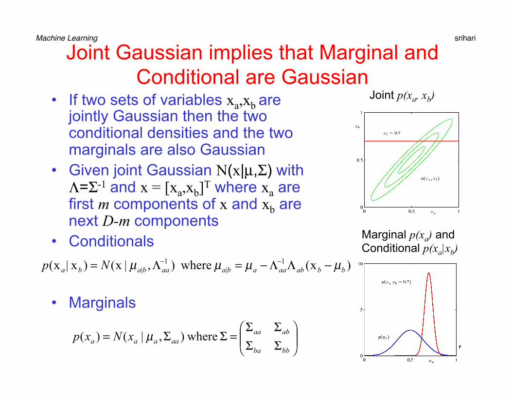
Joint Gaussian implies that Marginal and Conditional are Gaussian

•  If two sets of variables xa,xb are jointly Gaussian then the two conditional densities and the two marginals are also Gaussian

•  Given joint Gaussian N(x|µ,Σ) with Λ=Σ-1 and x = [xa,xb]T where xa are first m components of x and xb are next D-m components

•  Conditionals

•  Marginals

Joint p(xa, xb)

Marginal p(xa) and Conditional p(xa|xb)

)x( where),|x()x|x( 1|

1| bbabaaabaaababa Np µµµµ −ΛΛ−=Λ= −−

⎟⎟⎠

⎞⎜⎜⎝

⎛ΣΣΣΣ

=ΣΣ=bbba

abaaaaaaa xNxp where),|()( µ

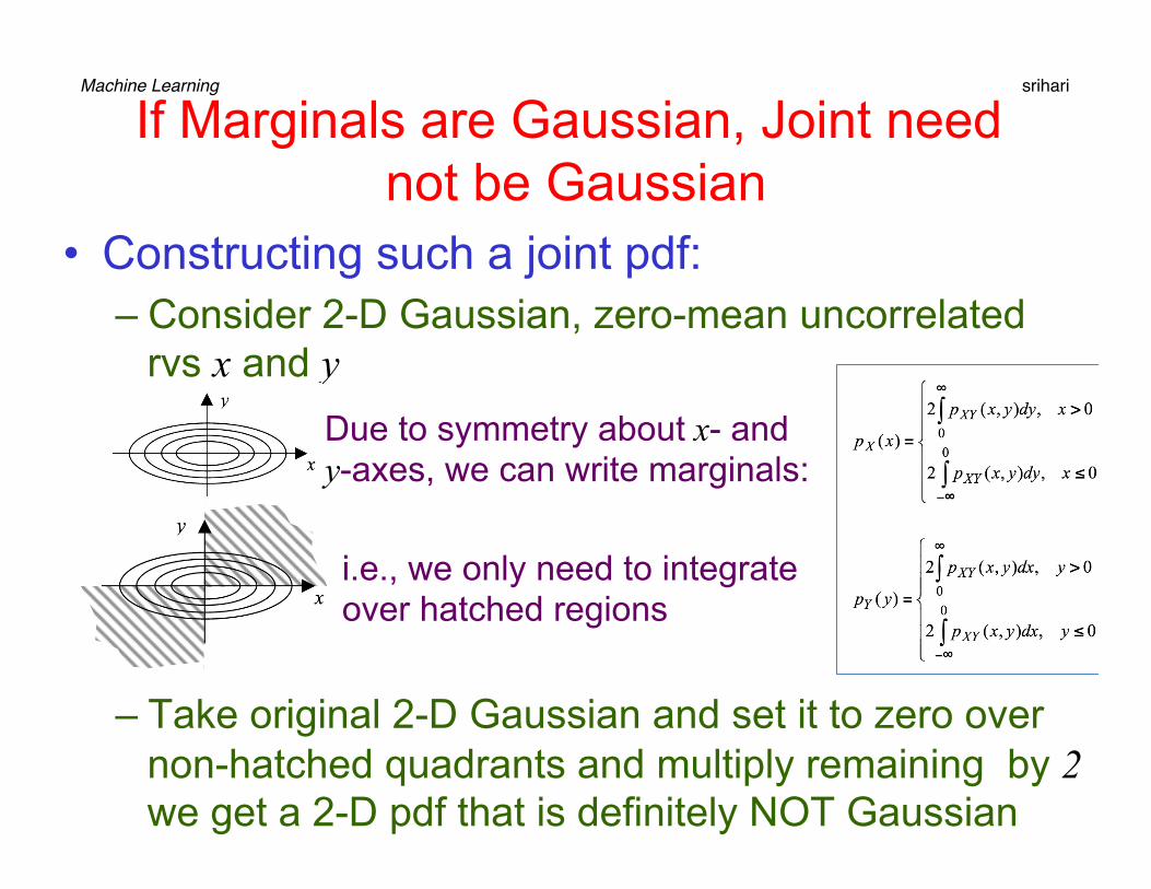
Machine Learning srihari If Marginals are Gaussian, Joint need

not be Gaussian •  Constructing such a joint pdf:

– Consider 2-D Gaussian, zero-mean uncorrelated rvs x and y

– Take original 2-D Gaussian and set it to zero over non-hatched quadrants and multiply remaining by 2 we get a 2-D pdf that is definitely NOT Gaussian

Due to symmetry about x- and y-axes, we can write marginals:

i.e., we only need to integrate over hatched regions


9

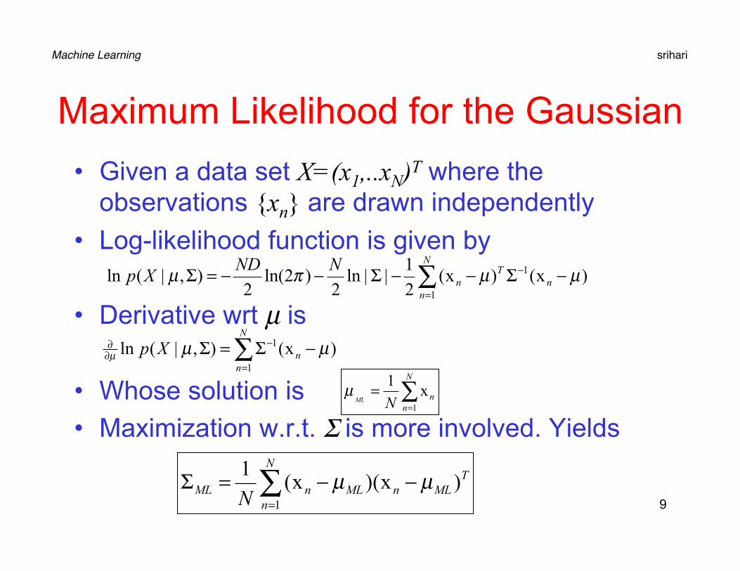
Maximum Likelihood for the Gaussian •  Given a data set X=(x1,..xN)T where the

observations {xn} are drawn independently •  Log-likelihood function is given by

•  Derivative wrt µ is

•  Whose solution is •  Maximization w.r.t. Σ is more involved. Yields

∑=

− −Σ−−Σ−−=ΣN

nn

Tn

NNDXp1

1 )x()x(21

||ln2

)2ln(2

),|( ln µµπµ

∑=

−∂∂ −Σ=Σ

N

nnXp

1

1 )x(),|( ln µµµ

∑=

=N

nnNML

1

x1µ

TMLn

N

nMLnML N

)x()x(1

1

µµ −−=Σ ∑=


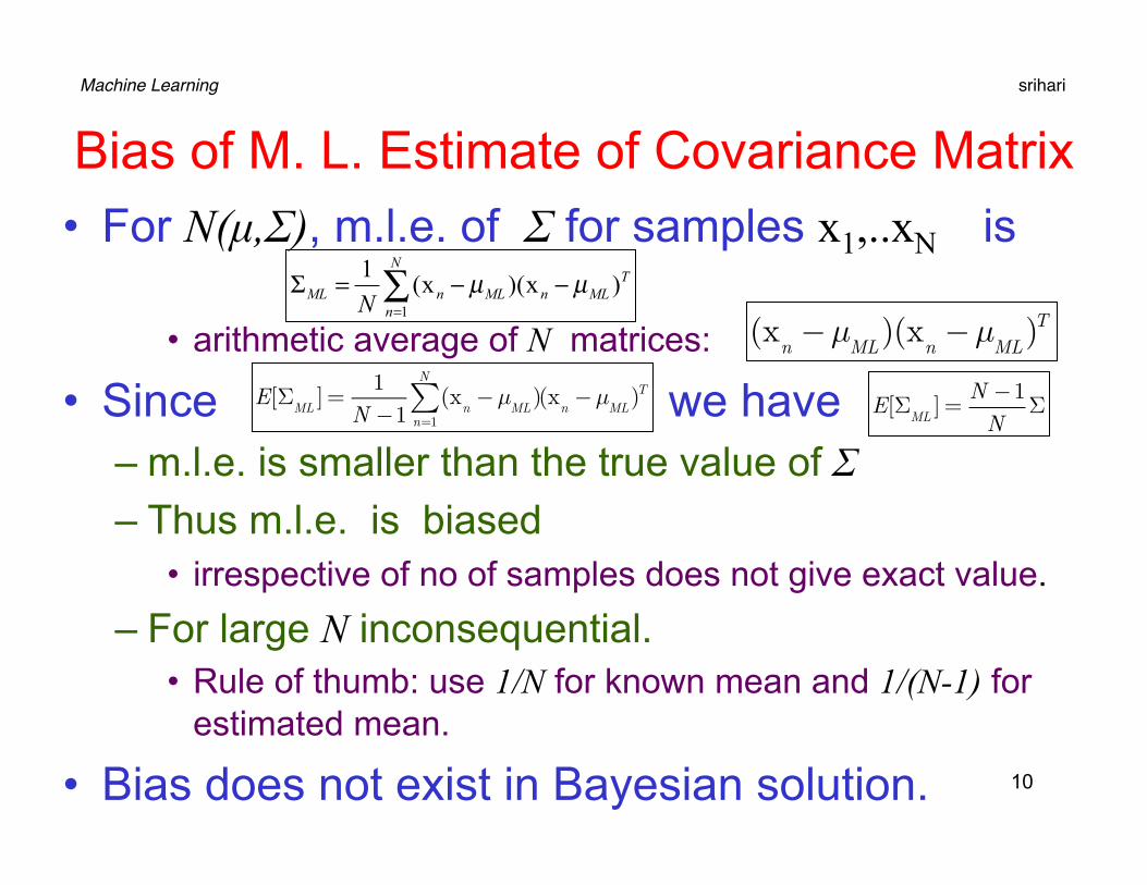
Bias of M. L. Estimate of Covariance Matrix •  For N(µ,Σ), m.l.e. of Σ for samples x1,..xN is

•  arithmetic average of N matrices:

•  Since we have – m.l.e. is smaller than the true value of Σ – Thus m.l.e. is biased

•  irrespective of no of samples does not give exact value. – For large N inconsequential.

•  Rule of thumb: use 1/N for known mean and 1/(N-1) for estimated mean.

•  Bias does not exist in Bayesian solution. 10

TMLn

N

nMLnML N

)x()x(1

1

µµ −−=Σ ∑=

(xn−µ

ML)(x

n−µ

ML)T

E[Σ

ML] =

1N −1

(xn−µ

ML)

n=1

N

∑ (xn−µ

ML)T E[Σ

ML]=N −1NΣ


11

Sequential Estimation •  In on-line applications and large data sets batch

processing of all data points in infeasible –  Real-time learning scenario where steady stream of

data is arriving and predictions must be made before all data is seen

•  Sequential methods allow data points to be processed one-at-a-time and then discarded –  Sequential learning arises naturally with Bayesian

viewpoint •  M.L.E. for parameters of Gaussian gives a

convenient opportunity to discuss more general discussion of sequential estimation for maximum likelihood


12

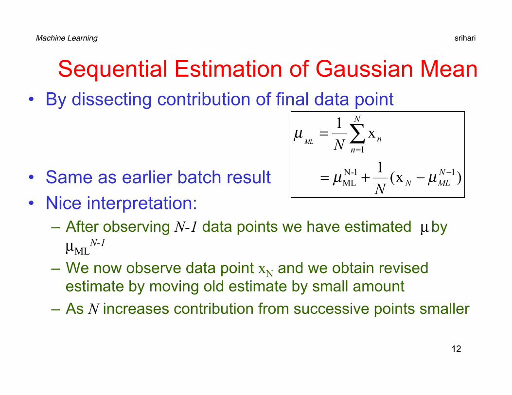
Sequential Estimation of Gaussian Mean •  By dissecting contribution of final data point

•  Same as earlier batch result •  Nice interpretation:

–  After observing N-1 data points we have estimated µ by µML

N-1

–  We now observe data point xN and we obtain revised estimate by moving old estimate by small amount

–  As N increases contribution from successive points smaller

)x(1

x1

11-NML

1

−

=

−+=

= ∑NMLN

N

nn

N

NML

µµ

µ


13

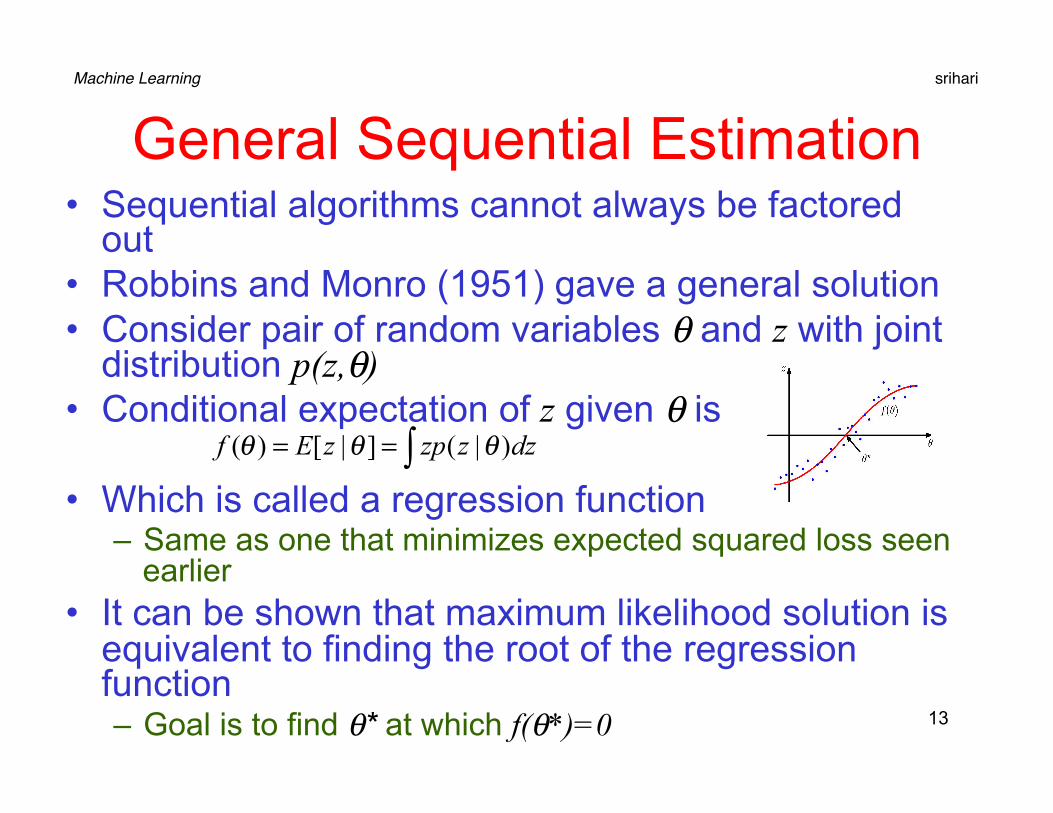
General Sequential Estimation •  Sequential algorithms cannot always be factored

out •  Robbins and Monro (1951) gave a general solution •  Consider pair of random variables θ and z with joint

distribution p(z,θ) •  Conditional expectation of z given θ is

•  Which is called a regression function –  Same as one that minimizes expected squared loss seen

earlier •  It can be shown that maximum likelihood solution is

equivalent to finding the root of the regression function –  Goal is to find θ* at which f(θ*)=0

∫== dzzzpzEf )|(]|[)( θθθ


14

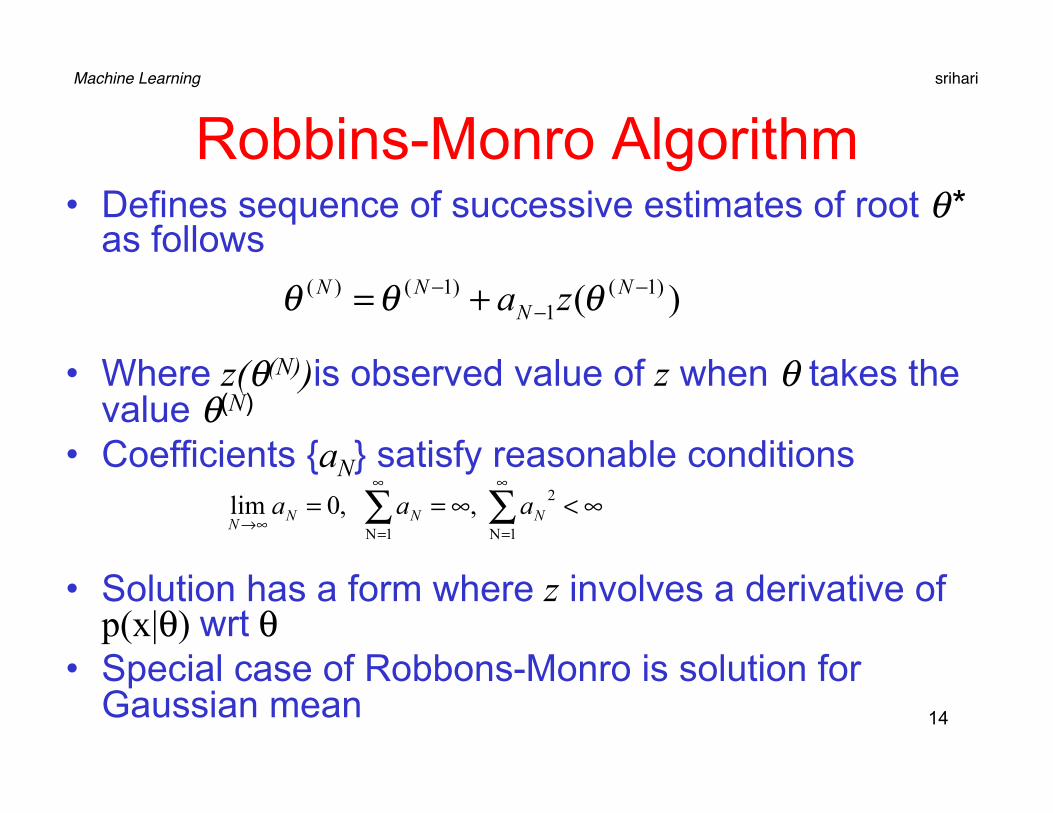
Robbins-Monro Algorithm •  Defines sequence of successive estimates of root θ*

as follows

•  Where z(θ(N))is observed value of z when θ takes the value θ(N)

•  Coefficients {aN} satisfy reasonable conditions

•  Solution has a form where z involves a derivative of p(x|θ) wrt θ

•  Special case of Robbons-Monro is solution for Gaussian mean

)( )1(1

)1()( −−

− += NN

NN za θθθ

∞<∞== ∑∑∞

=

∞

=∞→ 1N

2

1N , ,0lim NNNN

aaa


15

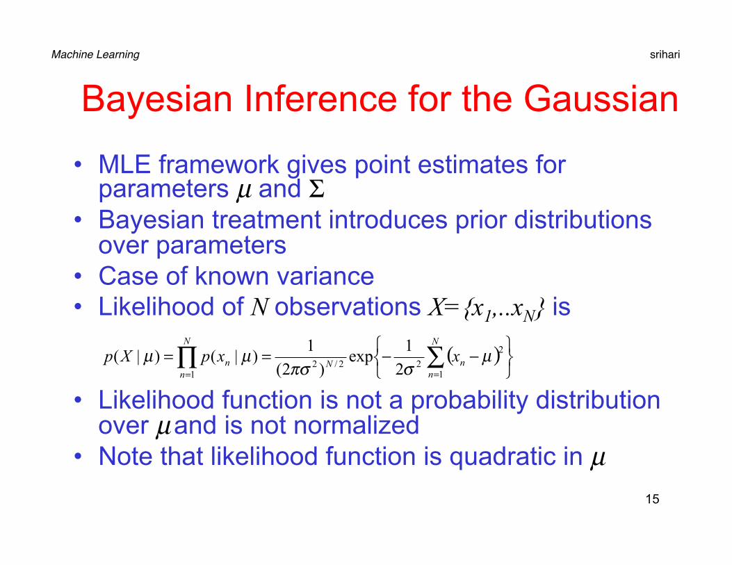
Bayesian Inference for the Gaussian

•  MLE framework gives point estimates for parameters µ and Σ

•  Bayesian treatment introduces prior distributions over parameters

•  Case of known variance •  Likelihood of N observations X={x1,..xN} is

•  Likelihood function is not a probability distribution over µ and is not normalized

•  Note that likelihood function is quadratic in µ

( )⎭⎬⎫

⎩⎨⎧ −−== ∑∏

==

N

nn

N

nNn xxpXp

1

22

12/2 2

1exp

)2(1

)|()|( µσπσ

µµ


16

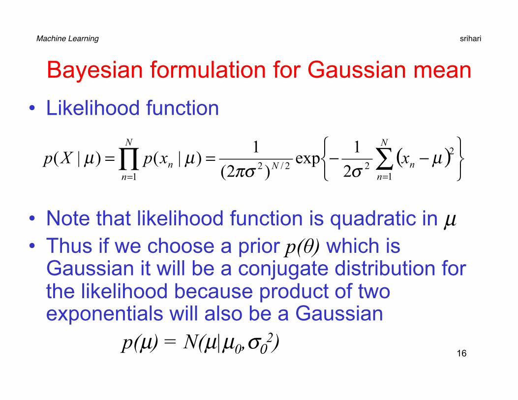
Bayesian formulation for Gaussian mean •  Likelihood function

•  Note that likelihood function is quadratic in µ•  Thus if we choose a prior p(θ) which is

Gaussian it will be a conjugate distribution for the likelihood because product of two exponentials will also be a Gaussian p(µ) = N(µ|µ0,σ0

2)

( )⎭⎬⎫

⎩⎨⎧ −−== ∑∏

==

N

nn

N

nNn xxpXp

1

22

12/2 2

1exp

)2(1

)|()|( µσπσ

µµ


17

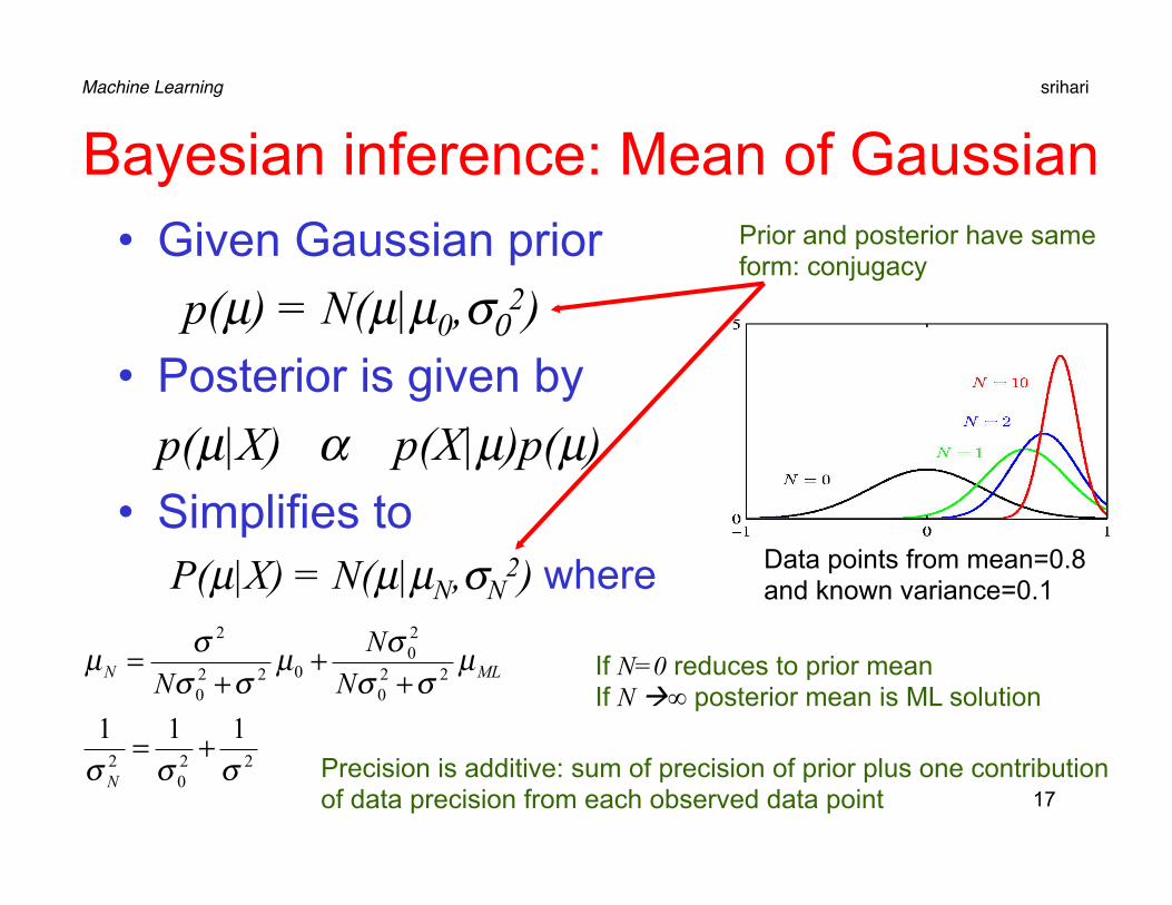
Bayesian inference: Mean of Gaussian •  Given Gaussian prior

p(µ) = N(µ|µ0,σ02)

•  Posterior is given by p(µ|X) α p(X|µ)p(µ)

•  Simplifies to P(µ|X) = N(µ|µN,σN

2) where

220

2

220

20

0220

2

111σσσ

µσσ

σµσσ

σµ

+=

++

+=

N

MLN NN

N

Precision is additive: sum of precision of prior plus one contribution of data precision from each observed data point

If N=0 reduces to prior mean If N à∞ posterior mean is ML solution

Data points from mean=0.8 and known variance=0.1

Prior and posterior have same form: conjugacy


18

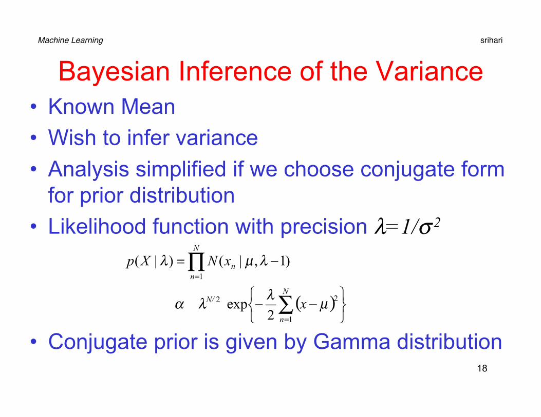
Bayesian Inference of the Variance •  Known Mean •  Wish to infer variance •  Analysis simplified if we choose conjugate form

for prior distribution •  Likelihood function with precision λ=1/σ 2

•  Conjugate prior is given by Gamma distribution

( )⎭⎬⎫

⎩⎨⎧ −−

−=

∑

∏

=

=

N

n

N/

N

nn

x

xNXp

1

22

1

2exp

)1,|()|(

µλλα

λµλ


19

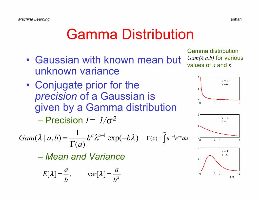
Gamma Distribution

•  Gaussian with known mean but unknown variance

•  Conjugate prior for the precision of a Gaussian is given by a Gamma distribution – Precision l = 1/σ 2

– Mean and Variance

)exp()(

1),|( 1 λλλ bb

abaGam aa −

Γ= −

Gamma distribution Gam(λ|a,b) for various values of a and b

2][ar v,][ba

baE == λλ

∫∞

−−=Γ0

1)( dueux ux


20

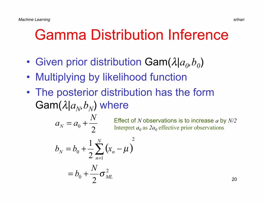
Gamma Distribution Inference

•  Given prior distribution Gam(λ|a0,b0) •  Multiplying by likelihood function •  The posterior distribution has the form

Gam(λ|aN,bN) where

( )

20

2

10

0

2

212

ML

N

nnN

N

Nb

xbb

Naa

σ

µ

+=

−+=

+=

∑=

Effect of N observations is to increase a by N/2 Interpret a0 as 2a0 effective prior observations


21

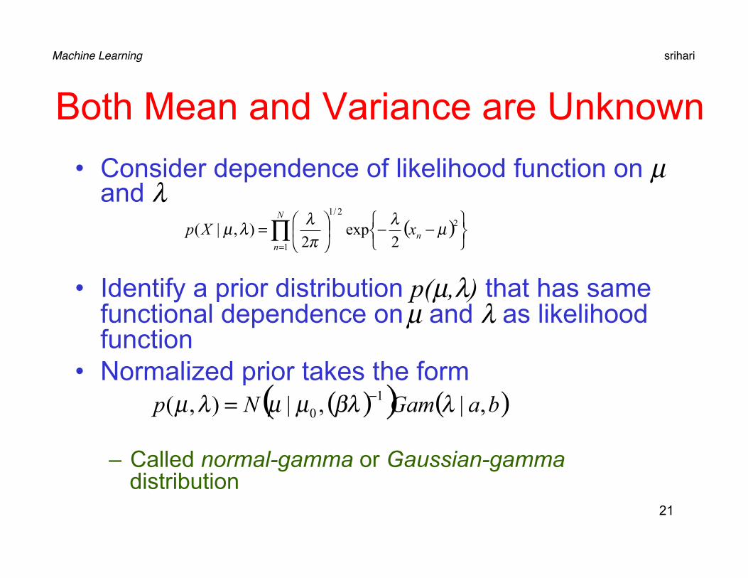
Both Mean and Variance are Unknown •  Consider dependence of likelihood function on µ

and λ

•  Identify a prior distribution p(µ,λ) that has same functional dependence on µ and λ as likelihood function

•  Normalized prior takes the form

–  Called normal-gamma or Gaussian-gamma distribution

( )∏= ⎭

⎬⎫

⎩⎨⎧ −−⎟

⎠⎞⎜

⎝⎛=

N

nnxXp

1

22/1

2exp

2),|( µλ

πλλµ

( )( ) ( )baGamNp ,|,|),( 10 λβλµµλµ −=


22

Normal Gamma

•  Both mean and precision unknown

•  Contour plot with µ0=0, β=2, a=5 and b=6


23

Estimation for Multivariate Case

•  For a multivariate Gaussian distribution N(x|µ,Λ-1) for a D-dimensional variable x – Conjugate prior for mean µ assuming known

precision is Gaussian – For known mean and unknown precision matrix Λ,

conjugate prior is Wishart distribution –  If both mean and precision are unknown conjugate

prior is Gaussian-Wishart


24

Student’s t-distribution •  Conjugate prior for precision of Gaussian is given by Gamma •  If we have a univariate Gaussian N(x|µ,τ -1) together with

Gamma prior Gam(τ|a,b) and we integrate out the precision we obtain marginal distribution of x

•  Has the form

•  Parameter ν=2a is called degrees of freedom and λ=a/b as the precision of the t distribution

ν à ∞ becomes Gaussian •  Infinite mixture of Gaussians with same mean but different

precisions –  Obtained by adding many Gaussian distributions –  Result has longer tails than Gaussian

∫∞

−=0

1 ),|(),|(),,|( τττµµ dbaGamxNbaxp

2/12/22/1 )(1)2()2/12/(),,|(

−−

⎥⎦

⎤⎢⎣

⎡ −+⎟⎠⎞⎜

⎝⎛

+Γ+Γ=

ν

νµλ

πνλ

νννλµ x

xSt


25

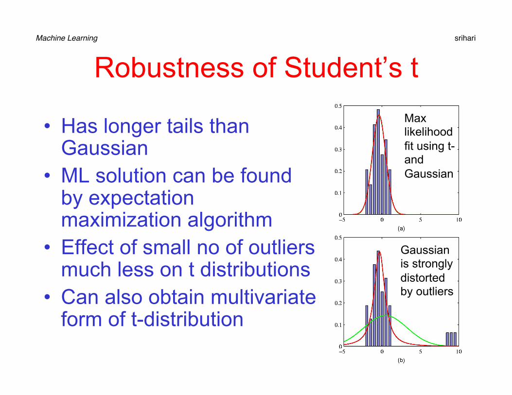
Robustness of Student’s t

•  Has longer tails than Gaussian

•  ML solution can be found by expectation maximization algorithm

•  Effect of small no of outliers much less on t distributions

•  Can also obtain multivariate form of t-distribution

Max likelihood fit using t- and Gaussian

Gaussian is strongly distorted by outliers


26

Periodic Variables •  Gaussian inappropriate for continuous variables that

are periodic or angular –  Wind direction on several days –  Calendar time –  Fingerprint minutiae direction

•  If we choose standard Gaussian, results depend on choice of origin –  With 0* as origin two observations θ1=1* and θ2=359* will

have mean at 180* and std dev 179* –  With 180* as origin mean=0*, std dev= 1*

•  Quantity represented by polar coordinates 0 < θ <2ρ


27

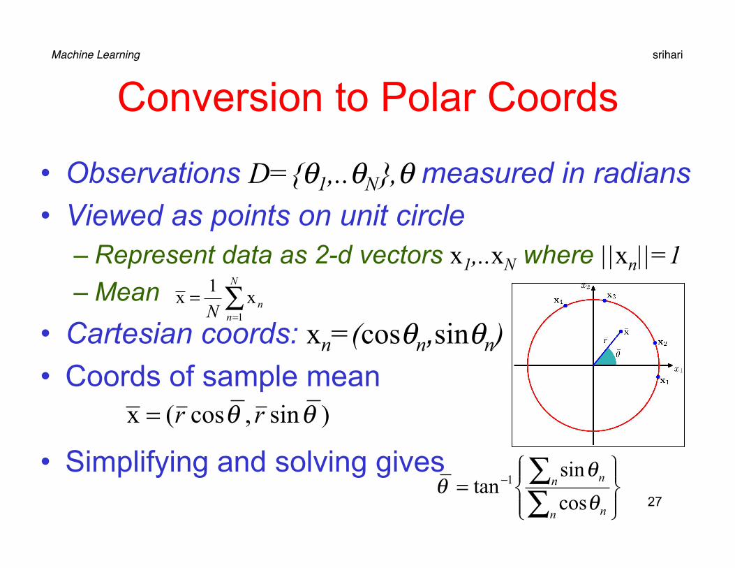
Conversion to Polar Coords

•  Observations D={θ1,..θN},θ measured in radians •  Viewed as points on unit circle

– Represent data as 2-d vectors x1,..xN where ||xn||=1 – Mean

•  Cartesian coords: xn=(cosθn,sinθn) •  Coords of sample mean

•  Simplifying and solving gives

∑=

=N

nnN 1

x1

x

)sin,cos(x θθ rr=

⎪⎭

⎪⎬⎫

⎪⎩

⎪⎨⎧

=∑∑−

n n

n n

θθ

θcos

sintan 1


28

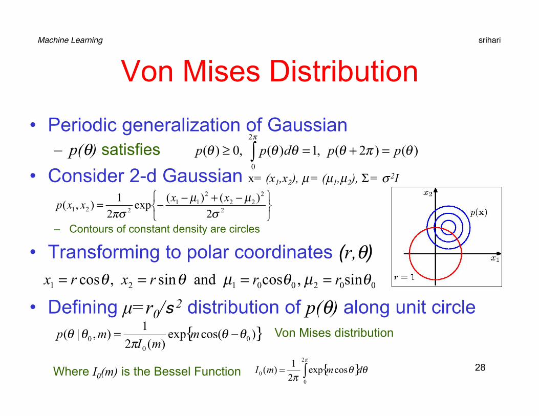
Von Mises Distribution

•  Periodic generalization of Gaussian –  p(θ) satisfies

•  Consider 2-d Gaussian x= (x1,x2), µ = (µ1,µ2), Σ = σ 2I

–  Contours of constant density are circles

•  Transforming to polar coordinates (r,θ)

•  Defining µ=r0/s 2 distribution of p(θ) along unit circle

⎭⎬⎫

⎩⎨⎧ −+−−= 2

222

211

221 2)()(

exp21

),(σ

µµπσ

xxxxp

∫ =+=≥π

θπθθθθ2

0

)()2( ,1)( ,0)( ppdpp

00200121 sin ,cos and sin ,cos θµθµθθ rrrxrx ====

{ })cos(exp)(2

1),|( 0

00 θθ

πθθ −= m

mImp Von Mises distribution

{ }θθπ

π

dmmI ∫=2

00 cosexp

21

)(Where I0(m) is the Bessel Function


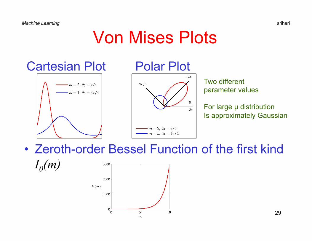
29

Von Mises Plots

•  Zeroth-order Bessel Function of the first kind I0(m)

Cartesian Plot Polar Plot Two different parameter values For large µ distribution Is approximately Gaussian


30

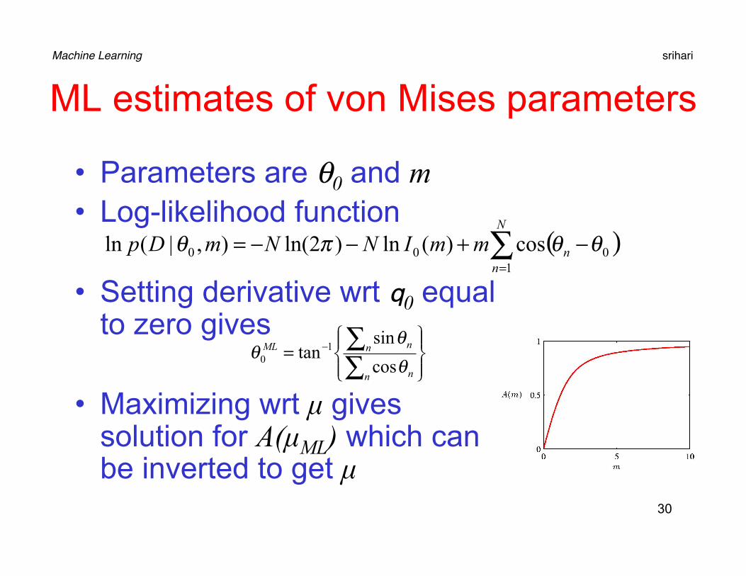
ML estimates of von Mises parameters

•  Parameters are θ0 and m •  Log-likelihood function

•  Setting derivative wrt q0 equal to zero gives

•  Maximizing wrt µ gives solution for A(µML) which can be inverted to get µ

( )∑=

−+−−=N

nnmmINNmDp

1000 cos)(ln)2ln(),|(ln θθπθ

⎪⎭

⎪⎬⎫

⎪⎩

⎪⎨⎧

=∑∑−

n n

n nML

θθ

θcos

sintan 1

0


31

Mixtures of Gaussians •  Gaussian has limitations in modeling real

data sets •  Old Faithful (Hydrothermal Geyser in

Yellowstone) –  272 observations –  Duration (mins, horiz axis) vs Time to next

eruption (vertical axis) –  Simple Gaussian unable to capture

structure –  Linear superposition of two Gaussians is

better •  Linear combinations of Gaussians can

give very complex densities

πk are mixing coefficients that sum to one

•  One –dimension –  Three Gaussians in blue –  Sum in red

∑=

Σ=K

kkkk xNp

1

),|()x( µπ


32

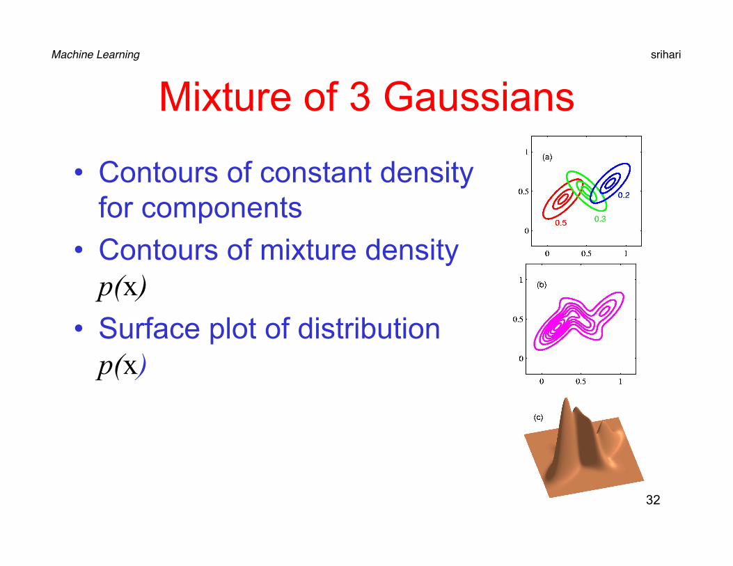
Mixture of 3 Gaussians

•  Contours of constant density for components

•  Contours of mixture density p(x)

•  Surface plot of distribution p(x)


33

Estimation for Gaussian Mixtures

•  Log likelihood function is

•  Situation is more complex •  No closed form solution •  Use either iterative numerical optimization

techniques or Expectation Maximization

( )∑ ∑= = ⎭

⎬⎫

⎩⎨⎧ Σ=Σ

N

n

K

kkknk NXp

1 1

,|xln),,|(ln µπµπ

Gaussian Distribution - Welcome to CEDAR€¦ · Machine Learning srihari 2 The Gaussian...

Documents

Transcript of Gaussian Distribution - Welcome to CEDAR€¦ · Machine Learning srihari 2 The Gaussian...