Thin elastic plates supported over small areas

II. Variational-asymptotic models.

G. Buttazzo∗, G.Cardone†, S.A.Nazarov‡

October 8, 2018

Abstract

An asymptotic analysis is performed for thin anisotropic elastic plate clamped along itslateral side and also supported at a small area θh of one base with diameter of the sameorder as the plate thickness h 1. A three-dimensional boundary layer in the vicinityof the support θh is involved into the asymptotic form which is justified by means of thepreviously derived weighted inequality of Korn’s type provides an error estimate with thebound ch1/2 |lnh| . Ignoring this boundary layer effect reduces the precision order down to

|lnh|−1/2. A two-dimensional variational-asymptotic model of the plate is proposed within

the theory of self-adjoint extensions of differential operators. The only characteristics of theboundary layer, namely the elastic logarithmic potential matrix of size 4 × 4, is involvedinto the model which however keeps the precision order h1/2 |lnh| in certain norms. Severalformulations and applications of the model are discussed.

Keywords: Kirchhoff plate, small support zone, asymptotic analysis, self-adjoint exten-sions, variational model.

MSC: 74K20, 74B05.

1 Introduction

1.1 Motivation

We consider a thin elastic anisotropic plate

Ωh =x = (y, z) ∈ R2 × R : y = (y1, y2) ∈ ω, |z| < h/2

(1.1)

∗Universita di Pisa, Department of Mathematics, Largo B. Pontecorvo, 5, 56127 Pisa, Italy; email: but-tazzo@dm.unipi.it.†Universita del Sannio, Department of Engineering, Corso Garibaldi, 107, 82100 Benevento, Italy; email:

giuseppe.cardone@unisannio.it.‡Mathematics and Mechanics Faculty, St. Petersburg State University, Universitetskaya nab., 7–9, St. Peters-

burg, 199034, Russia; Peter the Great Saint-Petersburg State Polytechnical University, Laboratory “Mechanicsof New Nano-materials”, Polytechnicheskaya ul., 29, St. Petersburg, 195251, Russia; Institute of Problems ofMechanical Engineering RAS, Laboratory “Mathematical Methods in Mechanics of Materials”, V.O., Bolshojpr., 61, St. Petersburg, 199178, Russia; email: s.nazarov@spbu.ru, srgnazarov@yahoo.co.uk.

1

arX

iv:1

601.

0491

2v1

[m

ath.

AP]

19

Jan

2016

y1 2

yz

h

hh

h

a)

b)

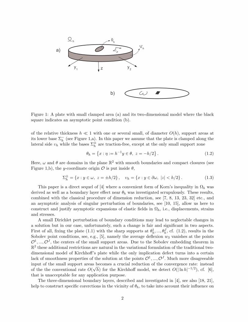
Figure 1: A plate with small clamped area (a) and its two-dimensional model where the blacksquare indicates an asymptotic point condition (b).

of the relative thickness h 1 with one or several small, of diameter O(h), support areas atits lower base Σ−h (see Figure 1,a). In this paper we assume that the plate is clamped along thelateral side υh while the bases Σ±h are traction-free, except at the only small support zone

θh =x : η := h−1y ∈ θ, z = −h/2

. (1.2)

Here, ω and θ are domains in the plane R2 with smooth boundaries and compact closures (seeFigure 1,b), the y-coordinate origin O is put inside θ,

Σ±h = x : y ∈ ω, z = ±h/2 , υh = x : y ∈ ∂ω, |z| < h/2 . (1.3)

This paper is a direct sequel of [4] where a convenient form of Korn’s inequality in Ωh wasderived as well as a boundary layer effect near θh was investigated scrupulously. These results,combined with the classical procedure of dimension reduction, see [7, 8, 13, 23, 32] etc., andan asymptotic analysis of singular perturbation of boundaries, see [10, 15], allow us here toconstruct and justify asymptotic expansions of elastic fields in Ωh, i.e., displacements, strainsand stresses.

A small Dirichlet perturbation of boundary conditions may lead to neglectable changes ina solution but in our case, unfortunately, such a change is fair and significant in two aspects.First of all, fixing the plate (1.1) with the sharp supports at θ1

h, ..., θJh , cf. (1.2), results in the

Sobolev point conditions, see, e.g., [5], namely the average deflexion w3 vanishes at the pointsO1, ...,OJ , the centers of the small support areas. Due to the Sobolev embedding theorem inR2 these additional restrictions are natural in the variational formulation of the traditional two-dimensional model of Kirchhoff’s plate while the only implication defect turns into a certainlack of smoothness properties of the solution at the points O1, ...,OJ . Much more disagreeableinput of the small support areas becomes a crucial reduction of the convergence rate: insteadof the the conventional rate O(

√h) for the Kirchhoff model, we detect O(| lnh|−1/2), cf. [6],

that is unacceptable for any application purpose.The three-dimensional boundary layers, described and investigated in [4], see also [18, 21],

help to construct specific corerctions in the vicinity of θh, to take into account their influence on

2

the far-field asymptotics and, as a result, to achieve the appropriate error estimate O(√h| lnh|).

At the same time, the global asymptotic approximation of the elastic fields becomes quitecomplicated so that its utility in application is rather doubtful. In this way, it is worth torestrict our analysis to the fair-field asymptotics whose dependence on the small parameter hremains complicated but can be expressed through rational functions in lnh and an integralcharacteristics of the support area, namely a 4× 4-matrix of elastic capacity [4, 18].

To provide a correct and mathematically rigorous two-dimensional model of the supportedplate, we employ two approaches. First, we turn to the technique of self-adjoint extensionsof differential operators (see the pioneering paper [1], the review [30] and, e.g., the papers[11, 17, 25, 29], especially [20] connecting this approach with the method of matched asymptoticexpansions). To simulate the influence of localized special boundary layer, we provide a properchoice of singular solutions by selecting a special self-adjoint extension in the Lebesgue spaceL2(ω) of the matrix L(∇y) of differential operators in the Kirchhoff plate model, see (2.30),(2.29). Parameters of this extension depend on the quantity | lnh| and the elastic logarithmiccapacity matrix, see [4, Sect. 3.2], which is similar to the logarithmic capacity in harmonicanalysis, cf. [12, 31].

The introduced model is two-fold and can be formulated as either an abstract equation withthe obtained self-adjoint operator, or a problem on a stationary point of the natural energyfunctional in a weighted function space with detached asymptotics. Advantages and deficienciesof these approaches are discussed in Section 3. In any case the compelled removal of a majorpart of the three-dimensional layer from the asymptotic form surely reduces capabilities of themodel which, in particular, does not give the global approximation of stresses and strains, butdoes outside a neighborhood of the sets θh and υh where the Dirichlet conditions are imposed.Thereupon, we mention that, first, the Kirchhoff model itself does not approximate correctlystresses and strains near the clamped edge, too, and, second, quite many applications demandto determine asymptotics of displacements only. In Corollaries 11 and 13 we will give someerror estimates for the model, in particular, an asymptotic formula for the elastic energy of thethree-dimensional thin-plate. Results [26] predict that the model also can furnish asymptoticsof eigenfrequencies of the plate but this will be a topic of an oncoming paper.

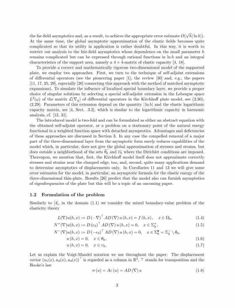
1.2 Formulation of the problem

Similarly to [4], in the domain (1.1) we consider the mixed boundary-value problem of theelasticity theory

L(∇)u(h, x) := D (−∇)>AD (∇)u (h, x) = f (h, x) , x ∈ Ωh, (1.4)

N+(∇)u(h, x) := D (e3)>AD (∇)u (h, x) = 0, x ∈ Σ+h , (1.5)

N−(∇)u(h, x) := D (−e3)>AD (∇)u (h, x) = 0, x ∈ Σ•h = Σ−h \ θh,u (h, x) = 0, x ∈ θh, (1.6)

u (h, x) = 0, x ∈ υh. (1.7)

Let us explain the Voigt-Mandel notation we use throughout the paper. The displacementvector (u1(x), u2(x), u3(x))> is regarded as a column in R3, > stands for transposition and theHooke’s law

σ (u) = Aε (u) = AD (∇)u (1.8)

3

relates the strain column

ε =(ε11, ε22, 2

1/2ε12, 21/2ε13, 2

1/2ε23, ε33

)>, εjk (u) =

1

2

(∂uj∂xk

+∂uk∂xj

),

with the stress column σ (u) of the same structure as ε (u) . Moreover, the stiffness matrix A ofsize 6× 6, symmetric and positive definite, figures in (1.8) as well as the differential operators

D (∇)> =

∂1 0 2−1/2∂2 2−1/2∂3 0 0

0 ∂2 2−1/2∂1 0 2−1/2∂3 0

0 0 0 2−1/2∂1 2−1/2∂2 ∂3

, ∂j =∂

∂xj, ∇ =

∂1

∂2

∂3

. (1.9)

The variational formulation of problem (1.4)-(1.7) implies the integral identity

(AD (∇)u,D (∇) v)Ωh= (f, v)Ωh

, ∀v ∈ H10 (Ωh; Γh)3 , (1.10)

where ( , )Ωhis the scalar product in L2 (Ωh) , H1

0 (Ωh; Γh) is a subspace of functions in the

Sobolev space H1 (Ωh) which vanish on Γh = θh∪υh, see (1.6) and (1.7), and the last superscript3 in (1.10) indicates the number of components in the test (vector) function v = (v1, v2, v3)> .

We here have listed only notation of further use while more explanation and an example ofthe isotropic material can be found in Section 1.2 of [4].

1.3 Architecture of the paper

In §2 we present the standard asymptotic procedure of dimension reduction to provide explicitformulas in the Kirchhoff plate’s model. Based on the results obtained in [4], we construct in§3 asymptotic expansions of a solution u(h, x) to problem (1.4)-(1.7) including the boundarylayer near the support area (1.2) and derive the error estimates in various versions.

The technique of self-adjoint extensions of differential operators is outlined in §3 for theKirchhoff plate supported at one point, i.e. with the Sobolev condition, together with thechoice of the extension parameters on the base of the previous asymptotic analysis. Finally, theasymptotic-variational model mentioned in Section 1.1 is discussed at length in §4.

2 The limit two-dimensional problem

2.1 The dimension reduction

We suppose that the right-hand side of system (1.4) takes the form

f (h, x) = h−1/2f0 (y, ζ) + h1/2f1 (y) + f (h, x) (2.1)

where ζ = h−1z ∈ (−1/2, 1/2) is the stretched transverse coordinate and f0, f1 are vectorfunctions subject to the conditions∫ 1/2

−1/2f0

3 (y, ζ) dζ = 0, f11 (y) = f1

2 (y) = 0, y ∈ ω. (2.2)

Now we assume f0 and f1 smooth and postpone a detailed description of properties of f0, f1

and f to Section 3.2. We emphasize that, owing to linearity of the problem, any reasonable

4

right-hand side can be represented as in (2.1), (2.2). After appropriate rescaling our choice ofthe factors h−1/2 and h1/2 in (2.1) as well as the orthogonality condition in (2.2) ensures thatthe potential energy stored by the plate Ωh under the volume force (2.1) gets order 1 = h0, seeSection 4.4.

As shown in [22], [23, Ch.4], the asymptotic ansatz

u (h, x) = h−3/2U0 (y) + h−1/2U1 (y, ζ) + h1/2U2 (y, ζ) + ... (2.3)

of the solution to problem (1.4)-(1.6) is perfectly adjusted with decomposition (2.1). Thecoordinate change x 7→ (y, ζ) splits the differential operators L (∇) and N± (∇) in (1.4) and(1.5), respectively, as follows:

L (∇) := D (−∇)>AD (∇) = h−2L0 (∂ζ) + h−1L1 (∇y, ∂ζ) + h0L2 (∇y) , (2.4)

N± (∇) := D (0, 0,±1)>AD (∇) = h−1N0± (∂ζ) + h0N1± (∇y) ,

where

L0 = −D>ζ ADζ , L1 = −D>ζ ADy −D>y ADζ , L2 = −D>y ADy,

N0± = ±D>3 ADζ , N1± = ±D>3 ADy

Dζ = D (0, 0, ∂ζ) , Dy = D (∇y, 0) , D3 = (0, 0, 1) , (2.5)

∂ζ = ∂/∂ζ, ∇y = (∂/∂y1, ∂/∂y2) .

We now insert formulas (2.4) and (2.3), (2.1) into (1.4) and (1.5) and collect coefficients ofhp−2 and hp−1, respectively. Equalizing their sums yields a recursive sequence of the Neumannproblems on the interval (−1/2, 1/2) 3 ζ with the parameter y ∈ ω. For p = 0, 1, 2, we have

L0Up = F p := −L1Up−1 − L2Up−2 for ζ ∈(−1

2 ,12

), (2.6)

N0±Up = Gp± := −N1±Up−1 at ζ = ±12 ,

where U−2 = U−1 = 0. Since F 0 = 0, G0± = 0 and F 1 = 0, G1± = ∓D>3 ADyU0, we readily

take

U0 (y) = w3 (y) e3, U1 (y) =2∑i=1

ei

(wi (y)− ζ ∂w3

∂yi(y)

)(2.7)

as solutions to problem (2.6) with p = 0 and p = 1. Here, ej is the unit vector of the xj-axisand

w = (w1, w2, w3)> (2.8)

is a vector function to be determined. Notice that h−3/2w3 (y) and h−1/2wi (y) will be theaveraged deflection and longitudinal displacements in the plate.

If p = 2, one may easily verify that the right-hand sides in (2.6) become

F 2 (y, ζ) = D>ζ ADyU1 +D>y A

(DζU

1 +DyU0)

= D>ζ AY (ζ)D (∇y)w (y) , (2.9)

G2± (y) = ∓D>3 AY (1/2)D (∇y)w (y)

where DζU1 +DyU

0 = 0 in view of (2.7) and

Y (ζ) =

(I3 −21/2I3ζO3 O3

), D (∇y)> =

∂1 0 2−1/2∂2 0 0 0

0 ∂2 2−1/2∂1 0 0 0

0 0 0 2−1/2∂21 2−1/2∂2

2 ∂1∂2

,

(2.10)

5

cf. (1.9), I3 and O3 are the unit and null matrices of size 3× 3.Hence,

U2 (y, ζ) = X (ζ)D (∇y)w (y) (2.11)

and X is a matrix solution (of size 3× 6) to the problem

−D>ζ ADζX (ζ) = D>ζ AY (ζ) , ζ ∈(−1

2 ,12

), ±D>3 ADζX

(±1

2

)= ∓D>3 AY

(±1

2

). (2.12)

Compatibility conditions in problem (2.12) are evidently satisfied.The problem with p = 3

L0Up = F p for ζ ∈(−1

2 ,12

), N0±Up = Gp± at ζ = ±1

2 (2.13)

gets the right-hand sides

F 3 = −L1U2 − L0U1 + f0 = D>ζ ADyU2 +D>y A

(DζU

2 +DyU1)

+ f0, (2.14)

G3± = ∓N1±U2 = ∓D>3 ADyU2.

Let us consider the compatibility conditions

Ipj (y) :=

∫ 1/2

−1/2F pj (y, ζ) dζ +Gp+j (y) +Gp−j (y) = 0, j = 1, 2, 3, (2.15)

with p = 3. By (2.14) and (2.7), (2.11), we have

DζU2 (y, ζ) +DyU

1 (y, ζ) = (DζX (ζ) + Y (ζ))D (∇y)w (y) (2.16)

and

I3i (y) = e>i D

>y

∫ 1/2

−1/2A (DζX (ζ) + Y (ζ)) dζD (∇y)w (y) dζ +

∫ 1/2

−1/2f0i (y, ζ) dζ.

Since e>i D>y = e>i D (∇y) according to (1.9), (2.5), (2.10), the equalities I3

i (y) = 0 with i = 1, 2are nothing but two upper lines in the system of differential equations

D (−∇y)>AD (∇y)w (y) = g (y) , y ∈ ω, (2.17)

where

A =

∫ 1/2

−1/2Y (ζ)>A (DζX (ζ) + Y (ζ)) dζ (2.18)

and

gi (y) =

∫ 1/2

−1/2f0i (y, ζ) dζ, i = 1, 2. (2.19)

6

The compatibility condition (2.15) with j = 3 is fulfilled automatically. Indeed, we take intoaccount the orthogonality condition in (2.2) and write

I33 (y) =

∫ 1/2

−1/2e>3 D

>y A (DζX (ζ) + Y (ζ)) dζ D (∇y)w (y)

=

2∑i=1

∂

∂yi

∫ 1/2

−1/2(Dζζei)

>A (DζX (ζ) + Y (ζ)) dζ D (∇y)w (y)

=

2∑i=1

∂

∂yi

(−∫ 1/2

−1/2e>i ζD

>ζ A (DζX (ζ) + Y (ζ)) dζ

+ e>i ζD>3 A (DζX (ζ) + Y (ζ))

∣∣∣1/2ζ=−1/2

)D (∇y)w (y) = 0.

Here, we again applied representation (2.16) together with the identity

Dye3 =

2∑i=1

Dζζei∂

∂yi(2.20)

inherited from (1.9), (2.5), and finally recalled problem (2.12) for the 3× 6-matrix X .Let us demonstrate that the third line of system (2.17) is equivalent to the equality

I43 (y) = 0, (2.21)

that is the third compatibility condition (2.15) in problem (2.13) with the right-hand sides

F 3 = −L1U3 − L0U2 + f1 = D>ζ ADyU3 +D>y A

(DζU

3 +DyU2)

+ f13 ,

G4± = ∓N1±U3 = ∓D>3 ADyU3.

We have

I43 (y) =

∫ 1/2

−1/2e>3 D

>y A

(DζU

3 +DyU2)dζ + f1

3 (2.22)

=

2∑i=1

∂

∂yi

∫ 1/2

−1/2(Dζζei)

>A(DζU

3 +DyU2)dζ + f1

3

= f13 +

2∑i=1

∂

∂yie>i

(−∫ 1/2

−1/2ζD>ζ A

(DζU

3 +DyU2)dζ +

(ζD>3 A

(DζU

3 +DyU2))|1/2ζ=−1/2

)

= f13 +

2∑i=1

∂

∂yie>i

∫ 1/2

−1/2ζ(D>y A

(DζU

2 +DyU1)

+ f0)dζ

= g3 +

2∑i=1

∂

∂yie>i D

>y

∫ 1/2

−1/2ζA (DζX + Y) dζD (∇y)w

where

g3 (y) = f13 (y) +

2∑i=1

∫ 1/2

−1/2ζ∂f0

i

∂yi(y, ζ) dζ. (2.23)

7

Let us clarify calculation (2.22). First, we used identity (2.20) and integrate by parts in theinterval (−1/2, 1/2) . Then we took into account problem (2.6) with p = 3 and its right-handsides (2.14). Finally, formula (2.16) was applied.

In view of (1.9) and (2.10) one observes that

2∑i=1

∂

∂yie>i D

>y ζ = e>3 D (∇y)Y (ζ)

and, hence, equality (2.21) indeed implies the third line of system (2.17) due to definition (2.18).

2.2 The plate equations

Owing to the Dirichlet condition (1.7) on the lateral side υh of the plate Ωh, we supply system(2.17) with the boundary conditions

wi (y) = 0, i = 1, 2, w3 (y) = 0, ∂nw3 (y) = 0, y ∈ ∂ω, (2.24)

where ∂n = n>∇y and n = (n1, n2)> is the unit vector of the outward normal at the boundaryof the domain ω ⊂ R2. Notice that conditions (2.24) make the main asymptotic terms (2.7) inansatz (2.3) vanish at the lateral boundary υh.

It follows from the weighted Korn’s inequality (2.10) in [4] and will be shown by other meanslater that the Dirichlet conditions (1.6) at the small support zones (1.2) lead to the Sobolev(point) condition at the y-coordinates origin O, namely

w3 (O) = 0. (2.25)

To prove the unique solvability of the limit two-dimensional problem (2.17), (2.24), (2.25) needsa piece of information on the matrix A of the system.

Lemma 1 Matrix (2.18) is block-diagonal and takes the form

A =

(A′ O3

O3 A(3)

)=

(A0 O3

O316A

0

)(2.26)

where A0 = A(yy)−A(yz)A−1(zz)A(zy) is a symmetric and positive definite 3×3-matrix constructed

from submatrices of size 3× 3 in the representation of the stiffness matrix

A =

(A(yy) A(yz)

A(zy) A(zz)

). (2.27)

Proof. We introduce the diagonal matrix J = diag(2−1/2, 2−1/2, 1

)and, by (2.27) and

(1.9), rewrite problem (2.12) as follows:

−A(zz)J∂2ζX (ζ) = A(zy)(O3,−21/2I3), ζ ∈ (−1/2, 1/2) ,

±A(zz)J∂ζX (±1/2) = ∓A(zy)(I3,∓21/2I3).

Its solution thus reads

X (ζ) = J−1A−1(zz)A(zy)

(−ζI3, 21/2

(ζ2

2 −124

)I3). (2.28)

8

Inserting this formula into (2.18) assures representation (2.26). Since matrix (2.27) is symmetricand positive definite, these properties are evidently passed to A0.

Representation (2.26) indicates a remarkable fact: for any homogeneous anisotropic platethe limit two-dimensional system (2.17) divides into the fourth-order differential operator

L3 (∇y) = 16D3 (∇y)>A0D3 (∇y) (2.29)

for the deflection w3 and the 2× 2-matrix second-order of differential operators

L′ (∇y) = D′ (−∇y)>A0D′ (∇y) (2.30)

for the longitudinal displacement vector w′ = (w1, w2)> .In the isotropic case (see formula (1.10) in [4]) we have

A0 =

λ′ + 2µ λ′ 0λ′ λ′ + 2µ 00 0 2µ

, λ′ =2λµ

λ+ 2µ

while L3 (∇y) and L′ (∇y) are the bi-harmonic operator and the plane Lame operator

L′3 (∇y) =µ

3

λ+ µ

λ+ 2µ∆2y, L′ (∇y) = −µ∆yI2 −

(λ′ + µ

)∇y∇>y .

Remark 2 Throughout the paper it is convenient to write the constructed solutions of problems(2.6) and (2.13) with f0 in the form

Up (y, ζ) = W p (ζ,∇y)w (y) , p = 0, 1, 2, 3, (2.31)

where, according to (2.7), (2.11) and (2.28),

W 0 (ζ,∇y) =

0 0 00 0 00 0 1

, W 1 (ζ,∇y) =

1 0 −ζ∂1

0 1 −ζ∂2

0 0 0

, ∂i =∂

∂yi, (2.32)

W 2 (ζ,∇y) = J−1A−1(zz)A(zy)

(−ζI3, 21/2

(ζ2

2− 1

24

)I3)D (∇y) .

A concrete formula for W 3 (ζ,∇y) will not be applied. We emphasize that (2.31) is a linearcombination of derivatives of w′ = (w1, w2) of order p− 1 and w3 of order p.

Proposition 3 Let

g3 = g03 −

2∑i=1

∂

∂yigi3, g0

3, gi3, gi ∈ L2 (ω) . (2.33)

Problem (2.17), (2.24), (2.25) admits a unique solution in the energy space H = H10 (ω; ∂ω)2×

H20 (ω; ∂ω ∪ O) . Moreover, this solution falls into H2 (ω)2 ×H3 (ω) and meets estimate

||w;H2 (ω)2 ×H3 (ω) || ≤ cN (2.34)

where N is the sum of norms of functions indicated in (2.33). The space H consists of vectorfunctions (2.8) in the direct product H1 (ω)2 ×H2 (ω) of Sobolev spaces such that the Dirichlet(2.24) and Sobolev (2.25) conditions are satisfied.

9

Proof. The variational formulation of problem (2.17), (2.24), (2.25) reads: to find w ∈ Hfulfilling the integral identity

(AD(∇y)w,D(∇y)v

)ω

=(g0

3, v3

)ω

+2∑i=1

((gi, vi)ω +

(gi3,

∂v3

∂yi

)ω

), ∀v ∈ H. (2.35)

The latter, as usual, is obtained by multiplying system (2.17) scalarly with a test function v ∈ Hand integrating by parts in ω with the help of conditions (2.24), (2.25) for v and the formulafor g3 in (2.33). Clearly, the right-hand side of (2.35) is a continuous linear functional in H 3 v.The left-hand side of (2.35) may be chosen as a scalar product in H. Indeed, the necessaryproperties of this bi-linear form are inherited from the positive definiteness of the matrix A0

together with the following Friedrichs and Korn inequalities:

||u;L2 (ω) || ≤ cω||∇yu;L2 (ω) ||, ∀u ∈ H10 (ω; ∂ω) , (2.36)

||∇yw′;L2 (ω) || ≤ cω||D′ (∇y)w′;L2 (ω) ||, ∀w′ ∈ H10 (ω; ∂ω)2 .

Equivalently, we may write equation (2.35) as the minimization problem

min

1

2

(AD(∇y)w,D(∇y)w

)ω− (g, w)ω : w ∈ H

where g = (g1, g2, g3) is given by (2.33). Notice that the Sobolev embedding theorem H2 ⊂ Cin R2 assures that H is a closed subspace in H1 (ω)2 × H2 (ω) and the second inequality in(2.36) can be easily derived by integration by parts because w′ vanishes at ∂ω.

Now the Riesz representation theorem guarantees the existence of a unique weak solutionto problem (2.35) and the estimate

||w;H1 (ω)2 ×H2 (ω) || ≤ cN .

Finally, a result in [14, Ch.2] on lifting smoothness of solutions to elliptic problems, see also [5]for details about the fourth-order equation, concludes with the inclusion w ∈ H2 (ω)2 ×H3 (ω)and inequality (2.34).

A classical assertion, cf. [7, 8, 13, 32] and others, was outlined in Theorem 7 of [4], namelythe rescaled displacements h3/2u3 (h, y, hζ) and h1/2ui (h, y, hζ) , i = 1, 2, taken from the three-dimensional problem (1.4)-(1.7), converge in L2 (ω × (−1/2, 1/2)) as h → +0 to the functionsw3 (y) and wi (y) − ζ ∂w3

∂yi(y) , respectively, where w = (w1, w2, w3)> is the solution of the two-

dimensional Dirichlet-Sobolev problem given in Proposition 3. Moreover, the convergence rateO(| lnh|−1/2), see Theorem 8 and Remark 6, is rather slow and in the next section we willimprove the asymptotic result by constructing three-dimensional boundary layers studied in[4, 18, 21].

3 Constructing and justifying the asymptotics

3.1 Matching the outer and inner expansions

Intending to apply the method of matched asymptotic expansions, cf. [10, 33] and [15, Ch.2],we regard (2.3) as the outer expansion suitable at a distance from the small support area (1.2).

10

In the vicinity of the set θh we, as mentioned in Section 3 of [4], use the stretched coordinates

ξ = (η, ζ) = (h−1y, h−1z) (3.1)

and engage the inner expansion in the form

u (h, x) = h1/2P (ξ) a+ ... (3.2)

where P is the elastic logarithmic potential, see Section 3.4 in [4], and a ∈ R4 is a column tobe determined. The decompositions for this potential derived in [4] show that, when ρ→ +∞,we have

h1/2P (ξ) a = h1/2( 3∑p=0

hpW p (ζ,∇η) Φ] (η) + d] (η, ζ)C])a+ ... = (3.3)

=

3∑p=0

hp−3/2W p (ζ,∇y)(

Φ] (y)−Ψ lnh+ d] (η, 0)C])a+ ...

Here, the operators W p(ζ,∇η) were introduced in Remark 2 and dots stand for lower-orderasymptotic terms and we have taken into account formulas

W p (ζ,∇η) = hp−1W p (ζ,∇y)H, H = diag1, 1, h, (3.4)

d] (η, ζ) = H−1d] (y, ζ) , Φ] (η) = H−1(

Φ] (y)− d] (y, 0) Ψ lnh)

where d] and Φ] are the following 3× 4-matrices

d] (η, ζ) =

1 0 0 ζ0 1 −ζ 00 0 η2 −η1

(3.5)

Φ] (y) =(d] (−∇y, 0)>Φ (y)>

)>=

Φ′ (y)

0 0

0 00 0

Φ23 (y) Φ1

3 (y)

, Φj3 =

∂Φ3

∂yj,

which are composed, respectively, from rigid motions and the nondegenerate block-diagonal4× 4-matrix

Ψ = diag

Ψ′,Ψ3,Ψ3

(3.6)

where Ψ′ is a non-degenerate numeral 2× 2-matrix and Ψ3 is a scalar in the representations

Φ′(y) = Ψ′ ln r + ψ′(ϕ), Φ3(y) = r2

(−1

2Ψ3 ln r + ψ3(ϕ)

)(3.7)

of the fundamental matrix of the differential operator (2.30) of size 2× 2 and the fundamentalsolution of the scalar differential operator (2.29). These were described in detail in Section 3.4of [4] on the base of general results in [9]. Moreover, (r, ϕ) is the polar coordinate system andψ′, ψ3 are smooth on the unit circle S1 3 ϕ. Furthermore, we have used the diagonal matrixH = diag 1, 1, h and the obvious formulas

d] (η, ζ) =(W 0 +W 1 (ζ,∇η)

)d] (η, 0) , W 2 (ζ,∇η) d] (η, 0) = W 3 (ζ,∇η) d] (η, 0) = 0. (3.8)

11

Note that lnh comes to (3.4) from the relation ln |η| = ln |y| − lnh and H is caused by differentorders of differentiation in W p (ζ,∇η) and different degrees of ρ = |η| in matrix functions butH disappears from the final expression in (3.3).

We also will need the following expansion of the elastic logarithmic potential, see Section3.6 in [4],

P(ξ) = (1− χθ(η))

(3∑p=0

W p (ζ,∇η) Φ] (η) + d] (η, 0)C] + Υ] (η)

)+˜P(ξ) (3.9)

which had been used in (3.3). Ingredients of (3.9) were defined in (2.32) and (3.5)-(3.7) while C]

stands for the elastic capacity matrix, χθ a smooth compactly supported function which equals1 in the vicinity of the clamped area θ, the vector function Υ] was described in Section 3.6 of

[4] but it plays an auxiliary role and an explicit form is not used below, and the remainders˜P

admits the estimates for a big ρ = |η|

|∇pη∂qζ˜P(ξ)| ≤ cpqρ−1+ε, |∇pη∂

qζ˜P3(ξ)| ≤ cpqρε, p, q = 0, 1, 2, ..., ε > 0. (3.10)

The presence of Φ] (y) drives all detached terms in (3.4) from the space H1 (ω)2×H2 (ω) wherethe solution w of the limit problem (2.17), (2.24), (2.25) was found in Proposition 3. On theother hand, the Neumann boundary condition (1.5) on the lower base Σ− does not hold onthe small set θh = Σ− \ Σ• which shrinks to the coordinate origin O. Hence, the dimensionreduction procedure in Section 2 was not able to deduce the differential equations at the pointO and we did not have a regular reason to cast out solutions with reasonable singularities. Letus introduce such solutions.

We denote by G′ the Green 2×2-matrix of the Dirichlet problem in ω for the matrix operator(2.30). Its particular value G′ (·,O) is a distributional solution of the problem

L′ (∇y)G′ (y,O) = δ (y) I2, y ∈ ω, G′ (y,O) = 0, y ∈ ∂ω, (3.11)

where δ is the Dirac mass and I2 is the unit 2× 2-matrix.As known, the Green function G3 of the Dirichlet problem for the fourth-order scalar dif-

ferential operator (2.29) belongs to H2 (ω) ⊂ C (ω) and its value

G3 (O,O) = (A3D3 (∇y)G3 (·,O) ,D3 (∇y)G3 (·,O))ω

is positive, see, e.g., [5]. The derivative in the second argument

G3,i (y,O) =∂

∂yiG3 (y,y) |y=0 (3.12)

leaves the space H2 (ω) but remains Holder-continuous in ω and satisfies the equation

L3 (∇y)G3.i (y,O) = − ∂

∂yiδ (y) , y ∈ ω, (3.13)

and the Dirichlet conditions (2.24). However, the Sobolev condition (2.25) is not achieved yetand we set

Gi3 (y,O) = G3,i (y,O)−G3,i (O,O)G3 (O,O)−1G3 (y,O) , (3.14)

12

cf. [5], so that Gi3 (O,O) = 0 and Gi3 (y,O) = ∂nGi3 (y,O) = 0, y ∈ ∂ω. Finally we introduce

the matrix function of size 3× 4

G] (y) =

G′ (y,O)

0 0

0 00 0

−G23 (y,O) G1

3 (y,O)

which, by virtue of (3.11) and (3.13), admits the representation

G] (y) = Φ] (y) + G] (y) (3.15)

where Φ] is the singular matrix function in (3.5) and G] is the regular part. According to general

properties of the Green matrices of second-order systems, see [9], first two lines G]i, i = 1, 2,

in G] involve smooth functions in ω, however the singularity O(r2 |ln r|

)of the subtrahend in

(3.14) moves some entries of G]3 from C2 (ω) but keep them still in the Holder space C1,α (ω)with any α ∈ (0, 1) . Hence, the remainder in (3.15) verifies the relations

G] (y) = d] (y, 0)G] + G] (y) , G]i (y) = O (r) , i = 1, 2, G]3 (y) = O(r2(1 + | ln r|)), (3.16)

where G] = G] (A,ω) is a numeric matrix of size 4 × 4. Properties of this matrix are just thesame as ones of the elastic logarithmic capacity and verification of its symmetry is a sufficientsimplification of the proof of Theorem 13 in [4].

Lemma 4 The 4× 4-matrix G] = G] (A,ω) in (3.16) is symmetric.

Let us put into the outer expansion (2.3) the singular solution

w (y) = w(y) +G](y)a (3.17)

of problem (2.17), (2.24), (2.25) with the same coefficient column a ∈ R4 as in (3.2) and thesmooth solution w ∈ H2 (ω)2 ×H3 (ω) given in Proposition 3. With a reference to the Sobolevembedding theorem H2 ⊂ C and the standard Hardy inequalities (see, e.g., Section 2.1 in [4]),we write

w (y) = d](y, 0)F + w(y) (3.18)

where the coefficient column F ∈ R4 and the remainder w satisfy the estimates

|F | ≤ cN , (3.19)∫ωr−2(1 + |ln r|)−2

(|∇yw′(y)|2 + r−2|w′(y)|2 + |∇2

yw3(y)|2 (3.20)

+r−2|∇yw3(y)|2 + r−4|w3(y)|2)dy ≤ cN ,

while N is the sum of norms of functions in (2.33).Notice that, according to definition of the Green matrix, we have

F =

∫ωG] (y) g (y) dy.

13

Using formulas (3.17), (3.18) and notation (2.31), we obtain for the outer expansion (2.3) that

h−3/23∑p=0

hpUp (y, ζ) = h−3/23∑p=0

hpW p (ζ,∇y)w (y) (3.21)

=3∑p=0

hp−3/2W p (ζ,∇y)(d] (y, 0)F +

(Φ] (y) + d] (y, 0)

)a)

+ ...

where dots again stand for lower-order asymptotic terms. The method of matched asymptoticexpansions requires that the expressions detached in (3.21) and (3.3), coincide with each other.This coincidence implies the system of linear algebraic equations

F + G]a = − lnh Ψa+ C]a (3.22)

and, thus,

a (lnh) =(|lnh|Ψ + C] (A, θ)− G] (A,ω)

)−1F. (3.23)

We here display the dependence of C] and G] on the stiffness matrix A and the domains θ andω. Since the matrix (3.6) is not degenerate, the matrix

M ] (lnh) = |lnh|Ψ + C] (A, θ)− G] (A,ω) (3.24)

is invertible for a small h ∈ (0, 1), too. Moreover, column (3.23) is a rational vector function in|lnh| = − lnh while clearly

a (lnh) = |lnh|−1 Ψ−1F +O(|lnh|−2). (3.25)

Formula (3.23) gives concrete expressions to all terms in (2.3), (3.17) and (3.2) so that ourformal construction of main terms in the outer and inner expansions is completed.

3.2 The final assumptions on the right-hand sides

To provide the necessary properties of the regular solution (3.18) of problem (2.17), (2.24),(2.25), we put the following requirement on terms in representation (2.1):

f0 ∈ L2(ω ×

(−1

2 ,12

))3, f1

3 ∈ H−1 (ω) . (3.26)

The latter inclusion, as usual, cf. [14], means that

f13 (y) = ∇>y

−→f 1

3 (y) + f130 (y) ,

−→f 1

3 =(f1

31, f132

)> ∈ L2 (ω)2 , f130 ∈ L2 (ω) . (3.27)

More precisely, the right-hand side (2.23) of the third equation in system (2.17) gives rise tothe continuous functional

(g3, v3)ω :=(f1

30, v3

)ω−

2∑i=1

(f1

3i +

∫ 1/2

−1/2ζf0i (·, ζ) dζ,

∂v3

∂yi

)ω

, v3 ∈ H10 (ω) . (3.28)

14

In view of (2.19), (3.26) and (3.28), (3.27) condition (2.33) in Proposition 3 is fulfilled so thatthe solution w ∈ H2 (ω)2 ×H3 (ω) meets estimate (2.34) where, as well as in (3.19), (3.20), Ncan be now fixed as

N =∥∥f0;L2

(ω ×

(−1

2 ,12

))∥∥+2∑p=0

∥∥f13p;L

2 (ω)∥∥ . (3.29)

For the remainder f in (2.1), we suppose that the expression

N = h−1/2| lnh|−1(h−1||s2

hS−1h2 f3;L2 (Ωh) ||+

2∑i=1

||shS−1h1 fi;L

2 (Ωh) ||)

(3.30)

gets the same order as the expression (3.29). Notice that weights

sh(y) = h+ dist(y, ∂ω), Shq(y) = (h2 + |y|2)−q/2(1 + | ln(h2 + |y|2)|)−1, q = 0, 1, (3.31)

come from the anisotropic Korn inequality (2.10) in [4] and make the norms on the right-handside of (3.30) much weaker that the common Lebesgue norms. The factor h−1/2 |lnh|−1 isconsistent with the final error estimate in Theorem 7. In other words, our way to signify thesmallness of this remainder does not spoil the precision of the two-dimensional model.

3.3 The global approximation solution

We proceed with constructing a vector function u ∈ H10 (Ωh; υh ∪ θh)3 which is a bit cumbersome

but very convenient for an estimation of the difference u−u between the true and approximatesolutions of problem (1.4)-(1.7). In the next section we will get rid of unnecessary terms in uto conclude a fair asymptotics of u.

Although in the previous section we have used the method of matched expansions, wenow apply an asymptotic structure attributed to the method of compound expansions, see acomparison of the methods in [15, Ch.2]. We give priority to expansion (3.2) and insert into(2.3) the decaying near O component w, see (3.18) and (3.20), instead of the whole singularsolution (3.17). We also introduce the cut-off functions

Xωh (y) = 1− χ

(h−1 |n|

), Xθ

h (y) = 1− χ(2h−1r/Rθ

)(3.32)

χ ∈ C∞ (R) , χ(r) = 1 for r < 12 , χ(r) = 0 for r ≥ 1, 0 ≤ χ ≤ 1,

which help to fulfill the Dirichlet conditions (1.7) and (1.6) because Xωh and Xθ

h vanish near theclamped sets υh and θh respectively. To this end, Rθ is fixed such that θ belongs to the diskB2R of radius R = Rθ.

We set

u (h, x) = h−1/2Xωh (y)P

(h−1x

)a (lnh) + (3.33)

+ h−3/2Xωh (y)

2∑p=0

hpW p (ζ,∇y)(Xθh (y) w (y)− hw (h, y)

)where the following correction term is introduced

w (h, y) =(1− χ

(R−1ω r))

Υ](h−1y

)(3.34)

15

with Υ] taken from (3.9) and Rω > 0 is such that BRω ⊂ ω. We emphasize that, accordingto definition of the differential operators (2.32) in (2.31), the inclusion w ∈ H2 (ω)2 × H3 (ω)assures that

W p (ζ,∇y) w ∈ H3−p (ω)3 for any ζ ∈ (−1/2, 1/2) (3.35)

and, therefore, the term W 3 (ζ,∇y) w (y) does not belong to the energy space H1 (Ωh)3 and isexcluded from the global approximation solution, i.e., p = 0, 1, 2 but p 6= 3 in (3.33).

Thanks to the cut-off functions (3.32) and the Dirichlet conditions for P, the displacementfield satisfies conditions (1.6), (1.7). Hence, the difference v = u−u ∈H1 (Ωh; υh ∪ θh)3 can betaken as a test function in the integral identity (1.10). Subtracting from both sides the scalarproduct (AD (∇)u, D (∇)v)Ωh

, we arrive at the formula

(AD (∇)v, D (∇)v)Ωh= (f,v)Ωh

− (AD (∇)u,v)Ωh. (3.36)

By the Korn inequality (see (2.10) and Theorem 2 in [4]), the left-hand side of (3.36) exceedthe product cA|||v; Ωh|||2• with the weighted anisotropic Sobolev norm

|||u; Ωh|||2• =

∫Ωh

(2∑i=1

(|∇yui|2 +

h2

s2h

S2h1

( ∣∣∣∣∂ui∂z

∣∣∣∣2 +

∣∣∣∣∂u3

∂yi

∣∣∣∣2 )+1

s2h

S2h1 |ui|

2)

(3.37)

+

∣∣∣∣∂u3

∂z

∣∣∣∣2 +h2

s4h

S2h2 |u3|2

)dx.

and our immediate objective becomes to examine the right-hand side. The complication arisesfrom the cut-off functions (3.32) which are included into (3.33) and meet the relations

|∇yXωh (y) | ≤ ch−1, supp |∇yXω

h | ⊂ ω (h) := y ∈ ω : 0 > n > −h , (3.38)

|∇yXθh (y) | ≤ ch−1, supp |∇yXθ

h| ⊂ B2Rωh.

Denoting vω = Xωh v and wθ = Xθ

hw, we obtain

||D (∇)vω;L2 (Ωh) || ≤ c(||D (∇)v;L2 (Ωh) ||+ h−1||v;L2 (ω (h)× (−h/2, h/2)) ||

)≤ C||D (∇)v;L2 (Ωh) || =: Cn,

||wθ;H2 (ω)2 ×H3 (ω) || ≤ c(||w;H2 (ω)2 ×H3 (ω) ||2 + J

)≤ c||w;H2 (ω)2 ×H3 (ω) ||2 ≤ CN ,

where J is the weighted integral on the left in (3.20). In both inequalities we have taken intoaccount that the weights sh (y) and r (1 + |ln r|) are small in the boundary strip ω (h) and thedisk B2Rθh.

16

3.4 Estimating the discrepancies

Let h−3/2XωhW − h−1/2Xω

hW stand for the last sum in (3.33). We have

(AD (∇)u, D (∇)v)Ωh= h−1/2 (AD (∇)Pa,D (∇)vω)Ωh

(3.39)

+ h−1/2(A (D (∇)Xω

h )(Pa+ h−1W −W

), D (∇)v

)Ωh

+(AD (∇)

(Pa+ h−1W −W

), (D (∇)Xω

h )v)

Ωh

+ h−1/2 (AD (∇)W, D (∇)vω)Ωh+ h−3/2 (AD (∇)W, D (∇)vω)Ωh

=: I1 + I2 + I3 + I4.

First of all, we observe that v = 0 at the lateral side υh and, therefore, after extending vω asnull over the layer R2 × (−h/2, h/2) we make the coordinate dilation (3.1) and integrate byparts to conclude that I1 = 0 since P is a solution of the homogeneous elasticity problem inthe infinite layer Λ = R2 × (−1/2, 1/2) clamped over the set θ × −1/2 on its lower base.

Next, formulas (3.9) and (3.17), (3.18) together with the matching condition (3.22) yield

P (ξ) a+ h−1W (h, x)−W (h, x)

=˜P (ξ) a+ h2

(W 3 (ζ,∇y) Φ] (η) + d] (η, 0)C] + Υ] (η)

)a+ h−1

2∑p=0

hpW p (ζ,∇y)w (y) .

The first term on the right is estimated by means of (3.10) noticing that ρ−1 = hr−1 = O (h) inthe thin boundary strip ω (h) . The second term and its derivatives become O

(h2 (1 + |lnh|)

)near the plate edge due to formulas (3.5), (3.8) and (3.25). Furthermore,∫

ω(h)

(s−2h

∣∣w′∣∣2 +∣∣∇yw′∣∣2 + s−4

h |w3|2 + s−2h |∇yw3|2 +

∣∣∇2yw3

∣∣2) dy≤ c

∫ω(h)

(∣∣∇yw′∣∣2 +∣∣∇2

yw3

∣∣2) dy≤ ch

(∥∥w′;H2(ω \ BRω/2

)∥∥2+∥∥w3;H3

(ω \ BRω/2

)∥∥2)

≤ chN

follows from formulas (3.20), (3.25), the standard Hardy inequalities (cf. Section 2.1 in [4]) andanother consequence of the Newton-Leibnitz formula with some fixed T ≥ Rω/2, namely∫ h

0|U (t)|2 dt =

∫ h

0

∫ T

t

∂

∂τ

(χ (τ/T )U (τ)2

)dτdt ≤ c

∫ h

0

∫ T

t

(∣∣∣∣dUdτ (τ)

∣∣∣∣2 + |U (τ)|2)dτdt

≤ ch∥∥U ;H1 (0, T )

∥∥2.

Estimating the matrix function D (∇)Xωh according to (3.38) and mentioning that, by virtue

of weight (3.31) in norm (3.37),∥∥(D (∇)Xωh )v;L2 (Ωh)

∥∥ ≤ c|||v;ω (h)× (−h/2, h/2) |||• ≤ cn,

17

we deduce that

|I2| ≤ ch−1/2h1/2(h−1h (1 + |lnh|)2 |a| (mes2 ω (h))1/2 (3.40)

+∥∥w;H1 (ω (h))2 ×H2 (ω (h))

∥∥2+ h2 (1 + |lnh|)2 |a| (mes2 ω (h))1/2 )n

≤ ch1/2 |lnh|n.

Note that, in the middle part of (3.40), h−1/2 is the original common factor, h1/2 comes fromintegration in z, mes2 ω (h) = O (h) and (1 + |lnh|)2 reduces finally to 1 + |lnh| due to theinequality |a (lnh)| ≤ c (1 + |lnh|)−1N inherited from (3.23), (3.19) and (3.25).

The third term I3 is examined in the simplest way. Indeed, formulas (2.32) and (2.11), (2.9)assure that

h−1/2D (∇)W (h, x) (3.41)

= h1/2((DζX (ζ) + Y (ζ))D (∇y)w (h, x) + hDyW2 (ζ,∇y)w (h, x))

and we readily obtain that|I3| ≤ ch1/2h1/2 |lnh| Nn.

Estimating the fourth term I4 in (3.39) follows the standard scheme in the theory of thinplates with a modification caused by the cut-off function Xθ

h present in (3.33). The functionwθ satisfies the system

L (∇y) wθ = gθ := Xθhg − [L(∇y), Xθ

h]

where [L, Xθh] is the commutator of the differential operator with the cut-off function Xθ

h. By(3.20) and (3.38), we have∫ω

(S2

1,h|(1−Xθh)g′|2 + h−2S2

2,h|(1−Xθh)g3|2

)dy ≤ ch2 (1 + |lnh|)2N , (3.42)∫

ωS2

1,h|[L′, Xθh]w′|2dy ≤ c

∫B2Rθh

(r + h)2 (1 +∣∣ln (r2 + h2

)∣∣)2 (h−4|w′|2 + h−2|∇yw′|2)dy

≤ ch2 |lnh|4N ,∫ωS2

2,h|[L3, Xθh]w3|2dy

≤ c∫B2Rθh

(r + h)4 (1 +∣∣ln (r2 + h2

)∣∣)2 (h−8|w3|2 + h−6|∇yw3|2 + h−4|∇2yw3|2 + h−2|∇3

yw3|2)dy

≤ ch2 |lnh|4N .

In these calculations we used that weights are small on the disk B2Rθh and coefficients of order kderivatives in the first- and third-order operators [L′, Xθ

h] and [L3, Xθh] are O(hk−2) and O(hk−4),

respectively. Returning to the notation in Section 2.2, we set Up (y, ζ) = W p (ζ,∇y) wθ (y) ,

18

p = 0, 1, 2, and, similarly to (3.41), write

I4 = h−5/2(ADζU

0, D (∇)vω)

Ωh+ h−3/2

(A(DζU

1 +DyU0), D (∇)vθ

)Ωh

(3.43)

+ h−1/2(A(DζU

2 +DyU1), D (∇)vθ

)Ωh

+ h1/2(ADyU

2, D (∇)vθ)

Ωh

= h−3/2(A (DζX + Y)D (∇y)wθ, Dζv

ω)

Ωh+ h−1/2

(A(DζU

2 +DyU1), Dyv

ω)

Ωh

+(ADyU

2, Dζvω)

Ωh+ h1/2

(ADyU

2, Dyvω)

Ωh

=: h−3/2I40 + h−1/2I41 + h1/2I42.

Here, we have taken into account that DζU0 = 0, DζU

1 +DyU0 = 0 due to (2.7) and, moreover,

I40 = 0 because the 3× 6-matrix X solves problem (2.12) and wθ is independent of ζ. Recallingproblem (2.13) with p = 3, we see that

I41 = −(D>y A

(DζU

2 +DyU1)

+D>ζ ADyU1,vθ

)Ωh

+∑± ±

(D>3 ADyU

2,vω)

Σ±h(3.44)

=(D>ζ ADζU

3 + f0,vω)

Ωh−∑± ±

(D>3 ADζU

3,vω)

Σ±h

=(f0,vω

)Ωh−(ADζU

3, Dζvω)

Ωh

=(f0,vω

)Ωh− h(ADζU

3, D (∇)vω)

Ωh+ h(ADζU

3, Dyvω)

Ωh.

We emphasize that the differential properties (3.35) put all entries of scalar products into theLebesgue space L2 (Ωh) . Furthermore, we have the estimates

h−1/2∣∣ (f0,vω

)Ωh−(f0,v

)Ωh

∣∣ = h−1/2

∣∣∣∣∣2∑i=1

(f0i , (1−Xω

h )vi)

Ωh

∣∣∣∣∣ (3.45)

≤ ch−1/2h1/2∥∥f0;L2 (Ω1)

∥∥h |||v;ω (h)× (−h/2, h/2) |||•≤ chNn,

h−1/2∣∣h(ADζU

3, D (∇)vω)

Ωh

∣∣ ≤ ch1/2h1/2N∥∥D (∇)vω;L2 (Ωh)

∥∥ ≤ chNn.

Notice that the factors h1/2 came into (3.45) due to the change z 7→ ζ = h−1z. It remains toconsider the last terms in (3.43) and (3.44). We write

h1/2(A(DyU

2 +DζU3), Dyv

ω)

Ωh= h1/2

(A(DyU

2 +DζU3), Dye3v

ω3

)Ωh

+h1/2(A(DyU

2 +DζU3), Dy (vω − e3v

ω3 ))

Ωh=: h1/2I1

42 + h1/2I242,

where vω3 (y) = h−1∫ h/2−h/2v

ω3 (y, z) dz. The known inequality∥∥Dy (vω − e3v

ω3 ) ;L2 (Ωh)

∥∥ ≤ ∥∥D (∇)vω;L2 (Ωh)∥∥ , ∀vω ∈ H1

0 (Ωh, υh)3 ,

see, e.g., [22, Section 4.3] and [23, Proposition 3.3.13], yields:

h1/2∣∣I2

42

∣∣ ≤ ch1/2h1/2Nn.

Finally, calculation (2.22) together with formulas (2.18), (2.26) for the matrix A and the re-lation D3 (∇y) = 2−1/2∇yD′ (∇y) between blocks in the matrix D (∇y) , see (2.10), demonstrate

19

that

h1/2I142 − h1/2

(f1

3 ,vω3

)Ωh

= h3/2

(2−1/2

(D′ (−∇y)>A(3)D3 (∇y) wθ3,∇yvω3

)ω

−(f1

30,vω3

)ω

+

2∑i=1

(f1

3i +Xθh

∫ 1/2

−1/2ζf0i (·, ζ) dζ,

∂vω3∂yi

)ω

).

We here took into account that in the approximate solution (3.33) the component w of (3.18)is multiplied with the cut-off function Xθ

h, see (3.32). Hence, to use the integral identity (2.35)with particular test functions vi = 0 and v3 = Xθ

hvω3 , which vanish in neighborhood of ∂ω and

O, we need to process several commutators with coefficient supports located in the small diskB2Rθh in the same way as we had done in (3.42). All of them receive bounds of similar order inh, always much better than in (3.40), and therefore we list only typical estimates

h3/2∣∣∣([D′ (∇y)>A(3)D3 (∇y) , Xθ

h

]w3,∇yvω3

)ω

∣∣∣≤ ch3/2

(∫B2Rθh

(h−6 |w3|2 + h−4 |∇yw3|2 + h−2

∣∣∇2yw3

∣∣2 )dy)1/2 ∥∥∇yvω3 ;L2 (B2Rθh)∥∥

≤ ch3/2 |lnh| Nh1/2∥∥∇yvω3 ;L2 (B2Rθh × (−h/2, h/2))

∥∥ ≤ ch |lnh|2Nn,

h3/2∣∣∣(f1

30,vω3

)ω−(f1

30, Xθhv

ω3

)ω

∣∣∣≤ ch3/2

∥∥f130;L2 (ω)

∥∥h1/2∥∥vω3 ;L2 (B2Rθh × (−h/2, h/2))

∥∥ ≤ ch2 |lnh|2Nn,

h3/2∣∣∣(f1

3i,vω3 ∂iX

θh

)ω

∣∣∣≤ ch3/2

∥∥f13i;L

2 (ω)∥∥h−3/2

∥∥vω3 ;L2 (B2Rθh × (−h/2, h/2))∥∥ ≤ ch |lnh|2Nn.

In this way we finally obtain:

h1/2∣∣I1

41 −(f1

3 ,vω3

)Ωh

∣∣ ≤ ch |lnh|2Nn.

We are in position to reckon calculations performed. Comparing bounds in all estimates forterms on the right of (3.39) we detect the worst one in (3.40), namely ch1/2 |lnh| Nn. Recallingalso supposition (3.30), we finally derive from (3.36) and (3.39), (2.1) the formula

(AD (∇)v, D (∇)v)Ωh≤ ch1/2 |lnh|

(N+N

) ∥∥D (∇)v;L2 (Ωh)∥∥

which together with the weighted anisotropic Korn inequality of Theorem 1 in [4] lead to thefollowing assertion.

Proposition 5 Under assumptions (2.2) and (3.26), (3.27) on the right-hand side (2.1) inproblem (1.4)-(1.7) (or (1.10) in the variational form) the difference v of the true u and ap-proximate u solutions meets the estimate

|||u− u; Ωh|||• ≤ c∥∥D (∇) (u− u) ;L2 (Ωh)

∥∥ ≤ Ch1/2 |lnh|(N+N

)(3.46)

where u is determined in (3.33), N and N in (3.29) and (3.30), ||| · |||• stands for the norm(3.37) and C is a constant independent of both, the right-hand side f and the small parameterh ∈ (0, h0] , h0 > 0.

20

Remark 6 As verified in [34], the error O(h1/2) of the Kirchhoff plate model (that is withoutthe small support (1.6)) cannot be improved because of the boundary layer phenomenon nearthe edge. We will see that the boundary layer near the support θh brings a perturbation of muchbigger order O(|lnh|−1).

3.5 Theorem on asymptotics

The complicated form (3.33) with various cut-off functions was technically needed to satisfy thestable boundary conditions (1.6) and (1.7) in the variational formulation (1.10) of the problembut after verifying estimate (3.46) we may get rid of some waste items while keeping the sameorder of proximity. We consider two versions of the simplified asymptotic structures, namely

uθ (h, x) = h−1/2P(h−1x

)a (lnh) + h−3/2

2∑p=0

hpW p (ζ,∇y) w (y) (3.47)

with the notation in (3.33) and

uω (h, x) = h−3/22∑p=0

hpW p (ζ,∇y)(w (y) +G]θ (h, x) a (lnh)

)+ h−1/2P

(h−1x

)a (lnh) (3.48)

where, comparing formula (3.15) with the content of Section 3.5 in [4], we set

G]θ (h, x) = (1− χ(r/2hRθ))Φ] (y) + G] (y) , (3.49)

P (ξ) = P (ξ)−2∑p=1

W p (ζ,∇η) (1− χ (ρ/2Rθ))(

Φ] (η) + d] (η, 0)C]).

Theorem 7 Under conditions of Proposition 5, the vector functions (3.47), (3.48) meet esti-mate (3.46).

Proof. According to (3.49), the approximate asymptotic solutions (3.47) and (3.48) differfrom each other only for the singular term, cf. (3.4),

(1− χ (2r/hRθ)) Φ] (y) = (1− χ (2ρ/Rθ))H(Φ] (η) + d] (η, 0) Ψ lnh),

and the concomitant rearranging of the rigid motion

h−1/2H−1d](y, 0)(C] −Ψ lnh)a (lnh) ,

taking into account the matching condition (3.22).Hence, it is sufficient to check up the estimate for uθ. First of all, we observe that the

discrepancy of (3.47) in the Dirichlet conditions (1.7) on the lateral side υh of the plate is equalto

h−3/22∑p=0

hpW p (ζ,∇y)HΥ](h−1y

)+ h−1/2 ˜P (ε−1x

)+ h1/2W 2 (ζ,∇y) w (y) . (3.50)

Fast decay of the first two terms in (3.50) and the small coefficient h1/2 in the third term allowus to withdraw from (3.33) the cut-off function Xω

h as well as term (3.34) which gets the small

21

factor h in (3.33) and vanishes in the disk BRω/2 3 y, that is at a distance from θh. This requires astandard and simple calculation based on weights in norm (3.37) and has been outlined in manypublications (see, e.g., [22], [23, §4.3] etc.). To take off from (3.33) the other cut-off function Xθ

h

which is null in the vicinity of θh, becomes much more delicate issue since the support of∣∣∇yXθ

h

∣∣is located very near singularities of the asymptotic terms. We make use of the weighted estimate(3.20) for w and observe that the expressions hp−3/2W p (ζ,∇y)

(1−Xθ

h (y))w (y) vanish outside

the cylinder B2Rθh × (−h/2, h/2) where all weights in (3.20) and (3.37) are big. In this way wewrite

hp−3/2|||W p(1−Xθh)w; Ωh|||•

≤ chp−3/2h1/2

(p−1∑q=0

h−(p−1−q)h−1 |lnh|−1 ||∇qyw′;L2(B2Rθh)||

+

p∑q=0

h−(p−q)h−1| lnh|−1||∇qyw3;L2(B2Rθh)||

)

≤ chp−1

(p−1∑q=0

h−(p−1−q)h1−q||r−2+q(1 + |ln r|)−1∇qyw′;L2(B2Rθh)||

+

p∑q=0

h−(p−q)h2−q||r−3+q(1 + |ln r|)−1∇qyw3;L2(B2Rθh)||

).

Note that the factors h1/2 and h−1| lnh|−1 arrived due to integration in z ∈ (−h/2, h/2) and tak-ing the weights Sh1 and hSh2 into account. Plugging into norms the weights r−2−q (1 + |ln r|)−1

and r−3−q (1 + |ln r|)−1 according to (3.20), we have gained back h2−q |lnh| and h3−q |lnh| ,respectively, that had led to the bound chN which is even better than in (3.46).

3.6 Further simplifications of asymptotic forms

By virtue of (3.20), (3.23) and the definition of the elastic capacity potential in [4], the elasticenergy of the boundary layer term h−1/2P

(h−1x

)a (lnh) in (3.48) gets order∥∥D (∇)h−1/2Pa;L2(Ωh)

∥∥2= O((h−1h3h−2|a (lnh) |2) = O(| lnh|−2) (3.51)

and therefore it cannot be omitted in the asymptotic expansion of the elastic fields in the plateΩh when one attends to achieve an error estimate with the power-law bound cδh

δ, δ > 0.However, contenting ourselves with the logarithmic precision O(|lnh|−1), we may write muchsimpler asymptotics.

Theorem 8 Under conditions of Proposition 5, the regular solution w ∈ H1 (ω)2 ×H2 (ω) ofthe two-dimensional Sobolev-Dirichlet problem (2.17),(2.24), (2.25) is related to the solutionu ∈ H1

0 (Ωh; Γh)3 of the three-dimensional problem (1.4)-(1.7) by the inequality

|||u− h−3/22∑p=0

hpW pw; Ωh|||• ≤ c |lnh|−1/2 (N+N ),

where W p (ζ,∇y) are differential operators in (2.32) and c is a constant independent of h ∈(0, h0] and quantities N , N given in (3.29), (3.30).

22

Proof. We still have to estimate the ingredients hp−3/2W p (ζ,∇y)G]θ (h, x) a (lnh) , p =0, 1, 2, of the asymptotic solution (3.34). We take into account representation (3.15) of theGreen matrix G] which is smooth in the punctured domain ω \ O and recall Remark 2 aboutW p (ζ,∇y) together with formulas (3.7), (3.5) for the fundamental matrix. Then we write

h−3/2|||G]θ3 a; Ωh|||• ≤ ch−3/2h1/2h

(1 +

∫ω\BRθh

(r2 (1 + |ln r|)2

(r2 + h2)2 (1 + |ln (r + h)|)2(3.52)

+(1 + |ln r|)2

(r2 + h2) (1 + |ln (r + h)|)2

)dy

)1/2

|a (lnh)|

≤ c |lnh|1/2 |lnh|−1 = c |lnh|−1/2 ,

h−1/2|||W 1G]θa; Ωh|||•

≤ ch−1/2h1/2

(1 +

∫ω\BRθh

(1 + |ln r|)2

(r2 + h2) (1 + |ln (r + h)|)2dy

)1/2

|a (lnh)| ≤ c |lnh|−1/2 ,

h1/2|||W 2G]θa; Ωh|||•

≤ ch1/2h1/2

(1 +

∫ω\BRθh

(1 + |ln r|)2

r2 (r2 + h2) (1 + |ln (r + h)|)2dy

)1/2

|a (lnh)| ≤ c |lnh|−1/2 .

For p = 0, we considered a specific input of the third component u3 into the weighted norm(3.37) while in the other cases p = 1, 2 the estimates were derived in the standard way: h1/2

comes from integration in z and 1 is inserted to bound the regular part of G]. Note that thefirst two integrals in (3.52) are O (|lnh|) while the third one is O

(h−1 |lnh|

)so that the relation

|a (lnh)| = O(|lnh|−1) is very important.

A similar effect of the catastrophic precision drop due to the Dirichlet condition at a smallregion was underlined in [6] for an homogenization problem in a perforated domain, too.

Our last simplification of asymptotic formulas is based on the following two observations.First,

||h−1/2Pa;L2 (Ωh) ||2 = O((h−1h3|a (lnh) |2) = O(h2| lnh|−2)

because the factors h−2 and h3 were introduced into (3.51) due to differentiation and integrationin the fast variables ξ = h−1x. Second, logarithmic singularities do not lead the Green matrixG] out from the spaces L2 (ω) and L2 (Ωh) . In other words, the boundary layer may be excludedfrom the asymptotic form but G] may be included without any cut-off function when dealingwith the Lebesgue norms of displacements (for stresses and strains this does not hold true, ofcourse).

Let us formulate a simple but substantial consequence of our previous results.

Theorem 9 Under conditions of Proposition 5, the inequality

2∑i=0

∥∥∥∥ui − h−1/2

(wi − h−1z

∂w3

∂yi

);L2 (Ωh)

∥∥∥∥+ h∥∥∥u3 − h−3/2w3;L2 (Ωh)

∥∥∥ ≤ ch1/2 |lnh| (N+N )

is valid where w (lnh;x) is the singular solution (3.17) of the two-dimensional problem (2.17),(2.24), (2.25) with the column a (lnh) ∈ R4 calculated in (3.23) and c is a constant independentof h ∈ (0, h0] and quantities N , N given in (3.29), (3.30).

23

4 A variational asymptotic model of a plate with small supports

4.1 A symmetric unbounded operator and its adjoint

We intend to apply a traditional scheme to model media with small defect in the frameworkof self-adjoint extension of differential operators, see the pioneering paper [1] together with thereview paper [30] where a physical terminology refers to ”potentials of zero radii”. Thanks tothe block-diagonal structure of the matrix L (∇y) , cf. Lemma 1, all preparatory results beloware substantiated by the papers [11] and [20] where a scalar fourth-order differential operatorand a second-order system are considered. At the same time, a straight way verification onthem is an accessible task, too.

Let A0 be an unbounded operator in the Hilbert space L2 (ω)3 with the differential expressionL (∇y) and the domain is

D(A0)

=w ∈ C∞c (ω \ O)3 : (2.24) is fulfilled

. (4.1)

Since the matrix L (∇y) is elliptic and block-diagonal, the closure A = A0 gets the samedifferential expression but the domain

D (A) =w ∈ H2 (ω)2 ×H4 (ω) : w (y) = 0, ∂nw3 (y) = 0, y ∈ ∂ω, (4.2)

w (O) = 0 ∈ R3, ∇yw3 (O) = 0 ∈ R2.

Here, the Sobolev theorem on embedding H2 ⊂ C is taken into account as well as the factthat H1 (ω) * C (ω) . In this way the property of w in (4.1) to vanish in a neighborhood of thecoordinate origin O were converted into five point conditions in (4.2) including the Sobolev one(2.25).

Both A0 and A are symmetric but not self-adjoint. Indeed, their adjoint operator A∗ keeps,as it is shown in [11, 20] and can be verified directly, the differential expression L (∇y) but itsdomain becomes much bigger, namely

D (A∗) =w = w(sing) + w(reg) : w(reg) ∈ H2 (ω)2 ×H4 (ω) , w(reg) (y) = 0, (4.3)

∂nw(reg)3 (y) = 0, y ∈ ∂ω, w′(sing) (y) = G′ (y,O) a′, a′ = (a1, a2)> ,

w′(sing)3 (y) = G3 (y,O) a0 +G13 (y,O) a3 +G2

3 (y,O) a4,

a0 ∈ R, a = (a1, a2, a3, a4)> ∈ R4.

Recall that the Green matrix G′ of problem (3.11) and the Green function G3 of the Dirichletproblem for the operator L3 (∇y) together with its derivatives (3.12) live in the Lebesgue spacebut higher-order derivatives do not. In particular, D (A∗) ⊂ L2 (ω)3 .

4.2 Self-adjoint extensions

One readily observes that codimension of the subspace D (A) ⊂ D (A∗) is 10 = 5+5, i.e. five freeconstants a0, ..., a4 in (4.3) and b0 = w(reg)3 (O) , b = d] (∇y, 0)w(reg) (O) ∈ R4. Moreover, thedefect index of A∗ equals (5 : 5), cf. [11, 20]. Hence, according to the von Neumann theorem,see [2, §4.4], the operator A admits self-adjoint extensions.

24

The Friedrichs extension (or the hard one, [2, §10.3]) is obtained, for example, as a restrictionof A∗ onto the subspace

w ∈ D (A∗) : a0 = 0, a = 0 ∈ R4

of codimension 5 and corresponds

to the classical formulation in H2 (ω)2 × H4 (ω) of problem (2.17),(2.24) with the right-handside g ∈ L2 (ω)3 . The Dirichlet-Sobolev problem (2.17),(2.24), (2.25), again with g ∈ L2 (ω)3 ,is associated with a self-adjoint extension possessing the domain

w ∈ D (A∗) : a = 0 ∈ R4, b0 = w3 (O) but a0 is arbitrary.

However, to realize modeling of the three-dimensional elasticity problem (1.4)-(1.7) in Ωh weought to deal with a different self-adjoint extension.

Theorem 10 Let M be a symmetric (real) 4 × 4-matrix. The restriction AM of A∗ onto thelinear space

D (AM ) =w ∈ D (A∗) : d] (∇y, 0)> w (O) =Ma, w3 (O) = 0, (4.4)

w (y) = w(reg) (y) + a0G (y,O)

is a self-adjoint extension of the operator A with domain (4.2).

Proof. To verify that (4.4) constitutes the domain of a self-adjoint operator, we first of allmention that D (A) ⊂ D (AM ) and dim (D (A∗) /D (AM )) = 5 because five linear restrictionsare imposed on the free coefficients in (4.3), namely on a, w(reg)3 (O) and d] (∇y, 0) w (O) =

(w1 (O) , w2 (O) , ∂1w3 (O) , ∂2w3 (O))>, see (3.5). Then the symplectic form

q (w, v) = (A∗w, v)ω + (w,A∗v)ω (4.5)

is properly defined on the direct product. At the same time, with a clear reason, form (4.5)vanishes in the case both w and v belong to the domain of a self-adjoint extension of A. Thus,if we confirm that q (w, v) = 0, ∀w, v ∈ D (AM ) the theorem is concluded.

We take functions from (4.3) with the attributes a(w), a(v) ∈ R4 and write

q (w, v) = limt→+0

((Lw, v)ω\Bt − (w,Lv)ω\Bt

)= lim

t→+0

( (N ′w′, v′

)St + (N3w3, (1,∇y) v3)St −

(w′,N ′v′

)St − ((1,∇y)w3,N3v3)St

)where Bt and St are the disk and circle with radius t and the center at y = 0 while theNeumann operators N ′ and N3 are taken from the Green formula for the differential operatormatrix L = diag L′,L3 in the domain ω \Bt with a small hole. Natural integration propertiesof the fundamental matrix (3.7), given, e.g., by formulas (3.36) and (3.42) in Section 3.4 in [4],provide a direct calculation of the last limit according to the representation in (4.3) and wefinally obtain

q (w, v) = (Lw, v)ω − (w,Lv)ω (4.6)

= (d] (∇y, 0)> v (O) + G]a(v))>a(w) − a>(w)

(d] (∇y, 0)> w (O) + G]a(w)

).

Since the matrices M and G] are symmetric, inserting relationship given in (4.4) shows thatthe right-hand side of (4.6) vanishes.

We call (4.6) the generalized Green formula, cf. [20, 28], [27, Ch.6]; it holds for any w, v ∈D (A∗) .

25

4.3 The operator model for the supported plate

We simplify representation (2.1) of the right-hand side in the three-dimensional problem (1.4)-(1.7) and set

f (h, x) = h−1/2(f0

1 (y) , f02 (y) , hf0

3 (y))>, f0

j ∈ L2 (ω) . (4.7)

The introduced restrictions (2.2) and (3.26), (3.27) are, of course, satisfied and, according to(2.19), (2.23), (3.29)

g (y) = f0 (y) =(f0

1 (y) , f02 (y) , f0

3 (y))>, N =

∥∥f0;L2 (ω)∥∥ , N = 0. (4.8)

Let A (lnh) be the self-adjoint operator AM](lnh) given by Theorem 10 with the numeralmatrix (3.24). We consider the abstract equation

A (lnh)w = g ∈ L2 (ω)3 . (4.9)

A solution of this equation takes form (3.17) where w ∈ H1 (ω)2 × H2 (ω) is the unique so-lution of the Sobolev-Dirichlet problem (2.17), (2.24), (2.25) and the column a = a (lnh) =M ] (lnh)−1 d] (∇y, 0) w (O) is perfectly defined through formulas (3.23) and (3.18) for a smallh > 0. In other words, the abstract equation (4.9) is uniquely solvable and, moreover, its solu-tion w ∈ D (A (lnh)) coincides with generator (3.17) of the outer asymptotic expansion (2.3)constructed in Sections 2.1 and 3.1.

Theorem 9 assures the following result.

Corollary 11 A solution w of equation (4.9) with the chosen self-adjoint extension A (lnh)and a right-hand side as in (4.7) and (4.8) satisfies the estimate∫

Ωh

2∑i=1

∣∣ui (h, x)− h−1/2wi (lnh, y)∣∣2 + h2

∣∣u3 (h, x)− h−3/2w3 (lnh, y)∣∣2dx ≤ ch1/2 |lnh| N

where N is given in (4.8) and c is a constant independent of data (4.7) and the small parameterε ∈ (0, ε0), ε0 > 0.

4.4 The variational model for the supported plate

The self-adjoint operator A (lnh) traditionally gives rise to the energy functional

12 (A (lnh)w,w)ω − (g, w)ω . (4.10)

We also introduce the functional

E (w; g) = 12 (A∗w,w)ω − (g, w)ω + 1

2a>(M ] (lnh) a− d] (∇y, 0) w (O)) (4.11)

which according to (4.4) at M = M ] (lnh) , coincides with (4.10) for v ∈ D (A (lnh)) but isdefined on the whole space

H =v ∈ D (A∗) : w3 (O) = 0

(4.12)

which becomes Hilbert with the norm

‖w;H‖ =(∥∥w(reg);H

2 (ω)2 ×H4 (ω)∥∥2

+ |a0|2 + |a|2)1/2

.

26

Theorem 12 A solution w ∈ D (A (lnh)) of equation (4.9) is the only stationary point offunctional (4.11) in H.

Proof. Since, by definition, A∗G] = 0 ∈ L2 (ω)4 , the generalized Green formula (4.6) andthe symmetry of the matrices M ] (lnh) and G] convert the variation of E into

1

2(Lw, v)ω +

1

2(Lv, w)ω − (g, v)ω +

1

2a>(v)

(M ] (lnh) a(w) − d] (∇y, 0) w (O)

)(4.13)

+1

2a>(w)

(M ] (lnh) a(v) − d] (∇y, 0) v (O)

)=

1

2(Lw, v)ω +

1

2(v,Lw)ω − (g, v)ω +

1

2a>(w)

(d] (∇y, 0) v (O) + G]a(v)

)− 1

2a>(v)

(d] (∇y, 0) w (O) + G]a(w)

)+

1

2a>(v)

(M ] (lnh) a(w) − d] (∇y, 0) w (O)

)+

1

2a>(w)

(M ] (lnh) a(v) − d] (∇y, 0) v (O)

)= (Lw − g, v)Ω + a>(v)

(M ] (lnh) a(w) − d] (∇y, 0) w (O)

).

Equating (4.13) to null and taking a test function v ∈ C∞c (ω \ O)3 yields

(Lw − g, v)Ω = 0 =⇒ L (∇y) w (y) = g (y) , y ∈ ω \ O,

while conditions (2.24) and (2.25) are inherited from the inclusion w ∈ H. Since a(v) ∈ R4 is ar-

bitrary, we conclude that expression (4.13) vanishes provided M ] (lnh) a(w) = d] (∇y, 0) w (O) .Thus, w falls into the domain D (A (lnh)) .

In a similar way one verifies that a solution w of (4.9) annuls the variation of functional(4.11).

From this theorem it follows that the abstract equation (4.9) is equivalent to the variationalproblem for the quadratic functional (4.11), cf. [16]. The latter is much more suitable for, e.g.,numerical implementation because the space (4.12) does not involve any linear restriction on wexcept for the Sobolev condition (2.25).

The potential energy of the three-dimensional plate (1.1) under the volume force (4.7) isequal to

Eh (u; f) = 12 (AD (∇x)u,D (∇x)u)Ωh

− (u, f)Ωh= −1

2 (u, f)Ωh;

here the Green formula for a solution u of (1.4)-(1.7) was applied. The last expression demon-strates that, although the introduced model cannot provide ”good” approximation of the strainand stress fields near the support area θh, Corollary 11 leads to a simple asymptotic formulafor the energy.

Corollary 13 For the right-hand sides (4.7) and (4.8), the solutions u (h, x) of the three-dimensional problem (1.4)-(1.7) and the solution w (lnh, y) of its two-dimensional model providethe following relationship between the corresponding energy functionals

|Eh (u; f)− E (w; g)| ≤ c√εN

where N is given in (4.8) and c is a constant independent of data (4.7) and the small parameterε ∈ (0, ε0) , ε0 > 0.

27

Modifying calculation (4.13) and applying the standard Green formula in ω, we derive that

E (w; g) = 12(Lw, w +G]a)ω − (g, w +G]a)ω + 0 (4.14)

= 12(Lw, w)ω − (g, w)ω − 1

2a>d (∇y, 0) w (O) + a>d (∇y, 0) w (O)

= E(w; g) + 12a>M ] (lnh) a,

where

E(w; g) =1

2(AD (∇y) w,D (∇y) w)ω − (g, w)ω. (4.15)

In other words, the energy functional (4.11) computed for the solution w ∈ D (A (lnh)) ofthe two-dimensional plate model (4.9) is equal to the sum of the potential energy (4.15), storedby the Kirchhoff plate with the Sobolev-Dirichlet conditions, and the correction term

1

2a>M ] (lnh) a (4.16)

which describes the energy concentrated in the vicinity of the small clamped zone θh. It shouldbe mentioned that, in view of (3.25) and (3.24), value (4.16) gets order O(|lnh|−1) and ispositive. The latter complies extension (1.2) of the Dirichlet area in the minimization problem

Eh (u; f) = minv∈H1

0 (Ωh;Γh)3Eh (v; f)

compared with the traditional problem on the plate (1.1) clamped along the lateral side υh.Although the model energy functional (4.14) gains the positive increment (4.16), the station-

ary point indicated in Theorem 12 does not constitute its minimum because of the calculation

E (w + v; g)− E (w; g) =1

2

(Lv, v +G]a(v)

)ω

+1

2a>(v)M

] (lnh) a(v)

=1

2(AD (∇y) v,D (∇y) v)ω +

1

2a>(v)

(M ] (lnh) a(v) − d] (∇y, 0) v (O)

)where the last terms can get any sign in H. This terms vanishes in D (A (lnh)) and, quiteexpected, the energy functional (4.11) admits the global minimum over the intrinsic linearspace (4.4) at the solution w of equation (4.9).

4.5 Conclusive remarks

Asymptotics derived and justified in §3 indicates a distinguishing feature of the influence of thesmall support θh on the strain-stress state of the plate Ωh, see (1.1) and (1.3). Namely, thethree-dimensional boundary layer phenomenon in the vicinity of θh overrides the standard errorestimateO(h1/2) for the two-dimensional Kirchhoff model and the convergence rateO(|lnh|−1/2)in

h1/2ui (h, y, hζ)→ wi (y)− ζ ∂w3

∂yi, i = 1, 2, (4.17)

h3/2u3 (h, y, hζ)→ w3 (y) in H1 (ω × (−1/2, 1/2)) ,

see Theorem 8, becomes too sluggish so that cannot maintain an engineering application. Anacceptable error estimate in Theorem 7, comparable with the usual one in the Kirchhoff theory,

28

requires to include into the asymptotic form the three-dimensional elastic field, that is theelastic logarithmical capacity potential P

(ε−1x

)in Section 3.5 of [4] which is not described

explicitly yet even for the disk θh of radius h and the isotropic material. However, replacingin (4.17) the regular solution w ∈ H1 (ω)2 × H2 (ω) of the Dirichlet-Sobolev problem (2.17),(2.24), (2.25) for the singular solution (3.17) procures the convergence rate O

(h1/2 |lnh|

)in

h1/2ui (h, y, hζ)− wi (lnh, y) + ζ ∂w3∂yi

(lnh, y)→ 0, i = 1, 2, (4.18)

h3/2u3 (h, y, hζ)− w3 (lnh, y)→ 0 in L2 (ω × (−1/2, 1/2)) ,

however in the Lebesgue, not Sobolev norm.The problem to determine the necessary singular solution w ∈ L2 (ω)2×H1 (ω) is well-posed

with different formulations in Sections 4.3 and 4.4. Its structure (3.17), (3.23) of w, refers tothe Green matrix (3.15), (3.16) and the integral characteristics C] (A, θ) in the representationof the logarithmic elastic potential P in the elastic layer, see Theorem 13 in [4]. The elasticlogarithmic capacity matrix is a numeral 4× 4-matrix and can be computed numerically.

Convergence (4.18) does not provide information about the stress and strain fields in theplate, however, using a technique of local estimates in [19, 23], it is possible to verify that, undercertain restrictions on the volume forces (3.26), this convergence becomes pointwise outside aneighborhood of θh. We mention that, as discovered in [34], see also [24], pointwise convergenceof stresses and strains is always broken near the clamped edge υh of the plate with or withoutsmall perturbation at θh.

Both, the asymptotic procedure and the models, can be easily adapted to the plate (1.1)with several small support areas θ1

h, ..., θJh sparsely distributed on one or two bases Σ±h .

In view of block-diagonal structure (2.26) of the matrix A the Dirichlet-Sobolev problem(2.17), (2.24), (2.25) naturally decouples into independent problems for the vector w′ = (w1, w2)of longitudinal displacements and the deflection w3. Since the elasticity problem for the infinitelayer Λ = R2 × (−1/2, 1/2) clamped over the only area θ × −1/2 loses the symmetry withrespect to the plane

ξ ∈ R3 : ξ3 = ζ = 0

, the elastic capacity matrix C] does not get in general

a block-diagonal structure and thus the relationship imposed in (4.4) on the regular and similarcomponents of the solution w = (w′, w3) of the model equation (4.9) couples the vector w′ andthe scalar w3 at the level O(|lnh|−1).

References

[1] Berezin F.A., Faddeev L.D., Remark on the Schrodinger equation with singular potential.Dokl. Akad. Nauk SSSR, 137 (1961) 1011–1014.

[2] Birman M. S., Solomyak M.Z., Spectral Theory of Self-Adjoint Operators in Hilbert Space.Reidel Publishing Company, Dordrecht, 1986.

[3] Bunoiu R., Cardone G., Nazarov S.A., Scalar boundary value problems on junctions of thinrods and plates. I. Asymptotic analysis and error estimates, ESAIM: Math. Model. Num.Anal., 48 (2014), 1495–1528.

[4] Buttazzo G., Cardone G., Nazarov S.A., Thin elastic plates supported over small areas. I.Korn’s inequalities and boundary layers. J. Convex Anal. 23 (1) (2016).

29

[5] Buttazzo G., Nazarov S.A., Optimal location of support points in the Kirchhoff plate. In:“Variational Analysis and Aerospace Engineering II”, Springer Optim. Appl. 33, Springer,New York, 2009, 33–48.

[6] Cardone G., Nazarov S.A., Piatnitski A.L., On the rate of convergence for perforated plateswith a small interior Dirichlet zone. Z. Angew. Math. Phys., 62 (3) (2011), 439–468.

[7] Ciarlet P.G., Plates and Junctions in Elastic Multi-Structures: An Asymptotic Analysis.Masson, Paris, and Springer-Verlag, Heidelberg, 1990.

[8] Ciarlet P.G., Mathematical Elasticity. Vol. II. Theory of Plates. Studies in Mathematicsand its Applications 27, North-Holland, Amsterdam, 1997.

[9] Gelfand I.M., Shilov G.E., Generalized Functions. Vol. 3: Theory of Differential Equations.Mayer Academic Press, New York-London, 1967.

[10] Il’in A.M., Matching of asymptotic expansions of solutions of boundary value problems.Translations of Mathematical Monographs 102, American Mathematical Society, Provi-dence, 1992.

[11] Karpeshina Y.E., Pavlov B.S., Interaction of the zero radius for the biharmonic and thepolyharmonic equation. Math. Notes, 40 (1-2) (1987), 528–533.

[12] Landkof N.S., Foundations of Modern Potential Theory. Die Grundlehren der mathema-tischen Wissenschaften 180, Springer-Verlag, New York-Heidelberg, 1972.

[13] Le Dret H., Problemes Variationnels dans les Multi-Domains Modelisation des Jonctionset Applications. Masson, Paris, 1991.

[14] Lions J.L., Magenes E., Non-Homogeneous Boundary Value Problems and Applications.Springer-Verlag, New York-Heidelberg, 1972.

[15] Maz’ya V.G., Nazarov S.A., Plamenevskij B.A., Asymptotic Theory of Elliptic BoundaryValue Problems in Singularly Perturbed Domains, Operator Theory. Advances and Appli-cations 112, Birkhauser Verlag, Basel, 2000.

[16] Mikhlin S.G., The problem of the minimum of a quadratic functional. Holden-Day Seriesin Mathematical Physics, Holden-Day, Inc., San Francisco-London-Amsterdam, 1965.

[17] Nazarov S.A., Self-adjoint extensions of the Dirichlet problem operator in weighted functionspaces. Math. USSR Sbornik, 65 (1) (1990), 229–247.

[18] Nazarov S.A. Elastic capacity and polarization of a defect in an elastic layer. Mekh. Tverd.Tela., 5 (1990), 57–65.

[19] Nazarov S.A., Justification of the asymptotic theory of thin rods. Integral and pointwiseestimates. J. Math. Sci., 97 (4) (1999), 4245–4279.

[20] Nazarov S.A., Asymptotic conditions at a point, self-adjoint extensions of operators andthe method of matched asymptotic expansions. Trans. Am. Math. Soc. Ser. 2, 193 (1999),77–126.

30

[21] Nazarov S.A., Asymptotic expansions at infinity of solutions to the elasticity theory problemin a layer. Trans. Moscow Math. Soc., 60 (1999), 1–85.

[22] Nazarov S.A., Asymptotic analysis of an arbitrary anisotropic plate of variable thickness(sploping shell). Sb. Math., 191 (7-8) (2000), 1075–1106.

[23] Nazarov S.A., Asymptotic Theory of Thin Plates and Rods. Vol.1. Dimension Reductionand Integral Estimates. Nauchnaya Kniga, Novosibirsk, 2001.

[24] Nazarov S.A., Estimates for second order derivatives of eigenvectors in thin anisotropicplates with variable thickness. J. Math. Sci., 132 (1) (2006), 91–102.

[25] Nazarov S.A., Asymptotic analysis and modeling of the jointing of a massive body with thinrods, J. Math. Sci., 127 (5) (2003), 2172–2263.

[26] Nazarov S.A., Asymptotics of solutions and modeling of the elasticity problems in a domainwith the rapidly oscillating boundary. Izv. Ross. Akad. Nauk. Ser. Mat., 72 (3) (2008), 103–158.

[27] Nazarov S.A., Plamenevsky B.A., Elliptic Problems in Domains with Piecewise SmoothBoundaries. Walter de Gruyter, Berlin-New York, 1994.

[28] Nazarov S.A., Plamenevskii B.A. A generalized Green’s formula for elliptic problems indomains with edges. J. Math. Sci., 73 (6) (1995), 674–700.

[29] Nazarov S.A., Sokolowski J. Self-adjoint extensions for the Neumann Laplacian and appli-cations. Acta Mathematica Sinica, 22 (3) (2006), 879–906.

[30] Pavlov B.S. The theory of extensions, and explicit solvable models. Russian Math. Surveys,42 (6) (1987) 127–168.

[31] Polya G., Szego G. Isoperimetric Inequalities in Mathematical Physics. Annals of Mathe-matics Studies 27, Princeton University Press, Princeton, 1951.

[32] Sanchez-Hubert J., Sanchez-Palencia E. Coques Elastiques Minces. Proprietes Asympto-tiques. Recherches en Mathematiques Appliquees 41, Masson, Paris, 1997.

[33] Van Dyke M. Perturbation methods in fluid mechanics, Applied Mathematics and Mechan-ics, Vol. 8 Academic Press, New York-London, 1964.

[34] Zorin I.S., Nazarov S.A. The boundary effect in the bending of a thin three-dimensionalplate, J. Appl. Math. Mech., 53 (4) (1989), 500–507.

31