Fundamentals Matrix Algebra
248
. of . Fundamentals . Matrix Algebra . . Third Edition . . . x . y . . . θ . Gregory Hartman
Transcript of Fundamentals Matrix Algebra
.
.
.
.
of.
Fundamentals
.
Matrix Algebra..
Third Edition
.
.. x.
y
.........
θ
.
Gregory Hartman

F M AThird Edi on, Version 3.1110
Gregory Hartman, Ph.D.Department of Mathema cs and Computer Science
Virginia Military Ins tute

Copyright © 2011 Gregory HartmanLicensed to the public under Crea ve CommonsA ribu on-Noncommercial 3.0 United States License

T
This text took a great deal of effort to accomplish and I owe a great many peoplethanks.
I owe Michelle (and Sydney and Alex) much for their support at home. Michelleputs up with much as I con nually read LATEX manuals, sketch outlines of the text, writeexercises, and draw illustra ons.
My thanks to the Department of Mathema cs and Computer Science at VirginiaMilitary Ins tute for their support of this project. Lee Dewald and Troy Siemers, mydepartment heads, deserve special thanks for their special encouragement and recog-ni on that this effort has been a worthwhile endeavor.
My thanks to all who informed me of errors in the text or provided ideas for im-provement. Special thanks to Michelle Feole and Dan Joseph who each caught a num-ber of errors.
This whole project would have been impossible save for the efforts of the LATEXcommunity. This text makes use of about 15 different packages, was compiled us-ing MiKTEX, and edited using TEXnicCenter, all of which was provided free of charge.This generosity helped convince me that this text should be made freely available aswell.
iii


PA Note to Students, Teachers, and other Readers
Thank you for reading this short preface. Allowme to share a few key points aboutthe text so that you may be er understand what you will find beyond this page.
This text deals with matrix algebra, as opposed to linear algebra. Without argu-ing seman cs, I view matrix algebra as a subset of linear algebra, focused primarilyon basic concepts and solu on techniques. There is li le formal development of the-ory and abstract concepts are avoided. This is akin to the master carpenter teachinghis appren ce how to use a hammer, saw and plane before teaching how to make acabinet.
This book is intended to be read. Each sec on starts with “AS YOU READ” ques onsthat the reader should be able to answer a er a careful reading of the sec on even ifall the concepts of the sec on are not fully understood. I use these ques ons as a dailyreading quiz for my students. The text is wri en in a conversa onal manner, hopefullyresul ng in a text that is easy (and even enjoyable) to read.
Many examples are given to illustrate concepts. When a concept is first learned,I try to demonstrate all the necessary steps so mastery can be obtained. Later, whenthis concept is now a tool to study another idea, certain steps are glossed over to focuson the newmaterial at hand. I would suggest that technology be employed in a similarfashion.
This text is “open.” If it nearly suits your needs as an instructor, but falls short inany way, feel free to make changes. I will readily share the source files (and help youunderstand them) and you can do with them as you wish. I would find such a processvery rewarding on my own end, and I would enjoy seeing this text become be er andeven eventually grow into a separate linear algebra text. I do ask that the Crea veCommons copyright be honored, in that any changes acknowledge this as a sourceand that it only be used non commercially.
This is the third edi on of the Fundamentals of Matrix Algebra text. I had notintended a third edi on, but it proved necessary given the number of errors found inthe second edi on and the other opportuni es found to improve the text. It variesfrom the first and second edi ons in mostly minor ways. I hope this edi on is “stable;”I do not want a fourth edi on any me soon.
Finally, I welcome any and all feedback. Please contact me with sugges ons, cor-rec ons, etc.
Sincerely,Gregory Hartman
v

Contents
Thanks iii
Preface v
Table of Contents vii
1 Systems of Linear Equa ons 11.1 Introduc on to Linear Equa ons . . . . . . . . . . . . . . . . . . . . 11.2 Using Matrices To Solve Systems of Linear Equa ons . . . . . . . . . 51.3 Elementary Row Opera ons and Gaussian Elimina on . . . . . . . . . 121.4 Existence and Uniqueness of Solu ons . . . . . . . . . . . . . . . . . 221.5 Applica ons of Linear Systems . . . . . . . . . . . . . . . . . . . . . 34
2 Matrix Arithme c 452.1 Matrix Addi on and Scalar Mul plica on . . . . . . . . . . . . . . . 452.2 Matrix Mul plica on . . . . . . . . . . . . . . . . . . . . . . . . . . 512.3 Visualizing Matrix Arithme c in 2D . . . . . . . . . . . . . . . . . . . 662.4 Vector Solu ons to Linear Systems . . . . . . . . . . . . . . . . . . . 802.5 Solving Matrix Equa ons AX = B . . . . . . . . . . . . . . . . . . . . 972.6 The Matrix Inverse . . . . . . . . . . . . . . . . . . . . . . . . . . . 1032.7 Proper es of the Matrix Inverse . . . . . . . . . . . . . . . . . . . . 112
3 Opera ons on Matrices 1213.1 The Matrix Transpose . . . . . . . . . . . . . . . . . . . . . . . . . . 1213.2 The Matrix Trace . . . . . . . . . . . . . . . . . . . . . . . . . . . . 1313.3 The Determinant . . . . . . . . . . . . . . . . . . . . . . . . . . . . 1353.4 Proper es of the Determinant . . . . . . . . . . . . . . . . . . . . . 1463.5 Cramer’s Rule . . . . . . . . . . . . . . . . . . . . . . . . . . . . . . 159
4 Eigenvalues and Eigenvectors 1634.1 Eigenvalues and Eigenvectors . . . . . . . . . . . . . . . . . . . . . . 1634.2 Proper es of Eigenvalues and Eigenvectors . . . . . . . . . . . . . . 177

Contents
5 Graphical Explora ons of Vectors 1875.1 Transforma ons of the Cartesian Plane . . . . . . . . . . . . . . . . . 1875.2 Proper es of Linear Transforma ons . . . . . . . . . . . . . . . . . . 2025.3 Visualizing Vectors: Vectors in Three Dimensions . . . . . . . . . . . 215
A Solu ons To Selected Problems 227
Index 237
viii
1 .
S L E
You have probably encountered systems of linear equa ons before; you can proba-bly remember solving systems of equa ons where you had three equa ons, threeunknowns, and you tried to find the value of the unknowns. In this chapter we willuncover some of the fundamental principles guiding the solu on to such problems.
Solving such systems was a bit me consuming, but not terribly difficult. So whybother? We bother because linear equa ons have many, many, many applica ons,from business to engineering to computer graphics to understandingmoremathemat-ics. And not only are there many applica ons of systems of linear equa ons, on mostoccasions where these systems arise we are using far more than three variables. (En-gineering applica ons, for instance, o en require thousands of variables.) So ge nga good understanding of how to solve these systems effec vely is important.
But don’t worry; we’ll start at the beginning.
1.1 Introduc on to Linear Equa ons
...AS YOU READ . . .
1. What is one of the annoying habits of mathema cians?
2. What is the difference between constants and coefficients?
3. Can a coefficient in a linear equa on be 0?
We’ll begin this sec on by examining a problem you probably already know howto solve.
.. Example 1 ..Suppose a jar contains red, blue and green marbles. You are toldthat there are a total of 30 marbles in the jar; there are twice as many red marbles as
Chapter 1 Systems of Linear Equa ons
green ones; the number of blue marbles is the same as the sum of the red and greenmarbles. How many marbles of each color are there?
S We could a empt to solve this with some trial and error, and we’dprobably get the correct answer without too much work. However, this won’t lenditself towards learning a good technique for solving larger problems, so let’s be moremathema cal about it.
Let’s let r represent the number of redmarbles, and let b and g denote the numberof blue and green marbles, respec vely. We can use the given statements about themarbles in the jar to create some equa ons.
Since we know there are 30 marbles in the jar, we know that
r+ b+ g = 30. (1.1)
Also, we are told that there are twice as many red marbles as green ones, so we knowthat
r = 2g. (1.2)
Finally, we know that the number of blue marbles is the same as the sum of the redand green marbles, so we have
b = r+ g. (1.3)
From this stage, there isn’t one “right” way of proceeding. Rather, there are manyways to use this informa on to find the solu on. One way is to combine ideas fromequa ons 1.2 and 1.3; in 1.3 replace r with 2g. This gives us
b = 2g+ g = 3g. (1.4)
We can then combine equa ons 1.1, 1.2 and 1.4 by replacing r in 1.1 with 2g as we didbefore, and replacing b with 3g to get
r+ b+ g = 30
2g+ 3g+ g = 30
6g = 30
g = 5 (1.5)
We can now use equa on 1.5 to find r and b; we know from 1.2 that r = 2g = 10and then since r+ b+ g = 30, we easily find that b = 15. ...
Mathema cians o en see solu ons to given problems and then ask “What if. . .?”It’s an annoying habit that we would do well to develop – we should learn to thinklike a mathema cian. What are the right kinds of “what if” ques ons to ask? Here’sanother annoying habit of mathema cians: they o en ask “wrong” ques ons. Thatis, they o en ask ques ons and find that the answer isn’t par cularly interes ng. Butasking enoughques ons o en leads to somegood “right” ques ons. So don’t be afraidof doing something “wrong;” we mathema cians do it all the me.
So what is a good ques on to ask a er seeing Example 1? Here are two possibleques ons:
2
1.1 Introduc on to Linear Equa ons
1. Did we really have to call the red balls “r”? Could we call them “q”?
2. What if we had 60 balls at the start instead of 30?
Let’s look at the first ques on. Would the solu on to our problem change if wecalled the red balls q? Of course not. At the end, we’d find that q = 10, and we wouldknow that this meant that we had 10 red balls.
Now let’s look at the second ques on. Suppose we had 60 balls, but the otherrela onships stayed the same. How would the situa on and solu on change? Let’scompare the “orginal” equa ons to the “new” equa ons.
Original Newr+ b+ g = 30 r+ b+ g = 60
r = 2g r = 2gb = r+ g b = r+ g
By examining these equa ons, we see that nothing has changed except the firstequa on. It isn’t too much of a stretch of the imagina on to see that we would solvethis new problem exactly the same way that we solved the original one, except thatwe’d have twice as many of each type of ball.
A conclusion fromanswering these two ques ons is this: it doesn’tma erwhatwecall our variables, and while changing constants in the equa ons changes the solu on,they don’t really change themethod of how we solve these equa ons.
In fact, it is a great discovery to realize that all we care about are the constants andthe coefficients of the equa ons. By systema cally handling these, we can solve anyset of linear equa ons in a very nice way. Before we go on, we must first define whata linear equa on is.
..Defini on 1
.
.Linear Equa on
A linear equa on is an equa on that can be wri en in theform
a1x1 + a2x2 + · · ·+ anxn = c
where the xi are variables (the unknowns), the ai arecoefficients, and c is a constant.
A system of linear equa ons is a set of linear equa ons thatinvolve the same variables.
A solu on to a system of linear equa ons is a set of valuesfor the variables xi such that each equa on in the system issa sfied.
So in Example 1, whenwe answered “howmanymarbles of each color are there?,”we were also answering “find a solu on to a certain system of linear equa ons.”
3
Chapter 1 Systems of Linear Equa ons
The following are examples of linear equa ons:
2x+ 3y− 7z = 29
x1 +72x2 + x3 − x4 + 17x5 =
3√−10
y1 + 142y4 + 4 = y2 + 13− y1√7r+ πs+
3t5
= cos(45◦)
No ce that the coefficients and constants can be frac ons and irra onal numbers(like π, 3
√−10 and cos(45◦)). The variables only come in the form of aixi; that is, just
one variable mul plied by a coefficient. (Note that 3t5 = 3
5 t, just a variable mul pliedby a coefficient.) Also, it doesn’t really ma er what side of the equa on we put thevariables and the constants, although most of the me we write them with the vari-ables on the le and the constants on the right.
We would not regard the above collec on of equa ons to cons tute a system ofequa ons, since each equa on uses differently named variables. An example of a sys-tem of linear equa ons is
x1 − x2 + x3 + x4 = 1
2x1 + 3x2 + x4 = 25
x2 + x3 = 10
It is important to no ce that not all equa ons used all of the variables (it is moreaccurate to say that the coefficients can be 0, so the last equa on could have beenwri en as 0x1 + x2 + x3 + 0x4 = 10). Also, just because we have four unknowns doesnot mean we have to have four equa ons. We could have had fewer, even just one,and we could have had more.
To get a be er feel for what a linear equa on is, we point out some examples ofwhat are not linear equa ons.
2xy+ z = 1
5x2 + 2y5 = 1001x+√y+ 24z = 3
sin2 x1 + cos2 x2 = 29
2x1 + ln x2 = 13
The first example is not a linear equa on since the variables x and y are mul -plied together. The second is not a linear equa on because the variables are raisedto powers other than 1; that is also a problem in the third equa on (remember that1/x = x−1 and
√x = x1/2). Our variables cannot be the argument of func on like sin,
cos or ln, nor can our variables be raised as an exponent.
4
1.2 Using Matrices To Solve Systems of Linear Equa ons
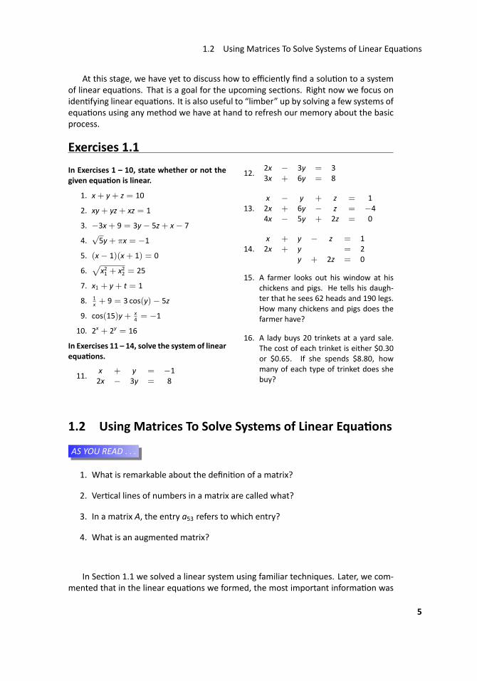
At this stage, we have yet to discuss how to efficiently find a solu on to a systemof linear equa ons. That is a goal for the upcoming sec ons. Right now we focus oniden fying linear equa ons. It is also useful to “limber” up by solving a few systems ofequa ons using any method we have at hand to refresh our memory about the basicprocess.
Exercises 1.1
In Exercises 1 – 10, state whether or not thegiven equa on is linear.
1. x+ y+ z = 10
2. xy+ yz+ xz = 1
3. −3x+ 9 = 3y− 5z+ x− 7
4.√5y+ πx = −1
5. (x− 1)(x+ 1) = 0
6.√
x21 + x22 = 25
7. x1 + y+ t = 1
8. 1x + 9 = 3 cos(y)− 5z
9. cos(15)y+ x4 = −1
10. 2x + 2y = 16
In Exercises 11 – 14, solve the system of linearequa ons.
11.x + y = −12x − 3y = 8
12.2x − 3y = 33x + 6y = 8
13.x − y + z = 12x + 6y − z = −44x − 5y + 2z = 0
14.x + y − z = 12x + y = 2
y + 2z = 0
15. A farmer looks out his window at hischickens and pigs. He tells his daugh-ter that he sees 62 heads and 190 legs.How many chickens and pigs does thefarmer have?
16. A lady buys 20 trinkets at a yard sale.The cost of each trinket is either $0.30or $0.65. If she spends $8.80, howmany of each type of trinket does shebuy?
1.2 Using Matrices To Solve Systems of Linear Equa ons
...AS YOU READ . . .
1. What is remarkable about the defini on of a matrix?
2. Ver cal lines of numbers in a matrix are called what?
3. In a matrix A, the entry a53 refers to which entry?
4. What is an augmented matrix?
In Sec on 1.1 we solved a linear system using familiar techniques. Later, we com-mented that in the linear equa ons we formed, the most important informa on was
5
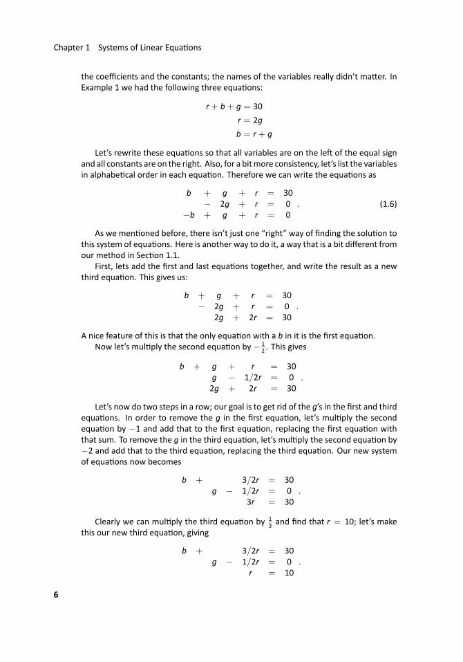
Chapter 1 Systems of Linear Equa ons
the coefficients and the constants; the names of the variables really didn’t ma er. InExample 1 we had the following three equa ons:
r+ b+ g = 30
r = 2g
b = r+ g
Let’s rewrite these equa ons so that all variables are on the le of the equal signand all constants are on the right. Also, for a bitmore consistency, let’s list the variablesin alphabe cal order in each equa on. Therefore we can write the equa ons as
b + g + r = 30− 2g + r = 0
−b + g + r = 0. (1.6)
As we men oned before, there isn’t just one “right” way of finding the solu on tothis system of equa ons. Here is another way to do it, a way that is a bit different fromour method in Sec on 1.1.
First, lets add the first and last equa ons together, and write the result as a newthird equa on. This gives us:
b + g + r = 30− 2g + r = 0
2g + 2r = 30.
A nice feature of this is that the only equa on with a b in it is the first equa on.Now let’s mul ply the second equa on by− 1
2 . This gives
b + g + r = 30g − 1/2r = 02g + 2r = 30
.
Let’s now do two steps in a row; our goal is to get rid of the g’s in the first and thirdequa ons. In order to remove the g in the first equa on, let’s mul ply the secondequa on by −1 and add that to the first equa on, replacing the first equa on withthat sum. To remove the g in the third equa on, let’s mul ply the second equa on by−2 and add that to the third equa on, replacing the third equa on. Our new systemof equa ons now becomes
b + 3/2r = 30g − 1/2r = 0
3r = 30.
Clearly we can mul ply the third equa on by 13 and find that r = 10; let’s make
this our new third equa on, giving
b + 3/2r = 30g − 1/2r = 0
r = 10.
6
1.2 Using Matrices To Solve Systems of Linear Equa ons
Now let’s get rid of the r’s in the first and second equa on. To remove the r in thefirst equa on, let’s mul ply the third equa on by − 3
2 and add the result to the firstequa on, replacing the first equa on with that sum. To remove the r in the secondequa on, we canmul ply the third equa on by 1
2 and add that to the second equa on,replacing the second equa on with that sum. This gives us:
b = 15g = 5
r = 10.
Clearly we have discovered the same result as when we solved this problem in Sec on1.1.
Now again revisit the idea that all that really ma ers are the coefficients and theconstants. There is nothing special about the le ers b, g and r; we could have used x,y and z or x1, x2 and x3. And even then, since we wrote our equa ons so carefully, wereally didn’t need to write the variable names at all as long as we put things “in theright place.”
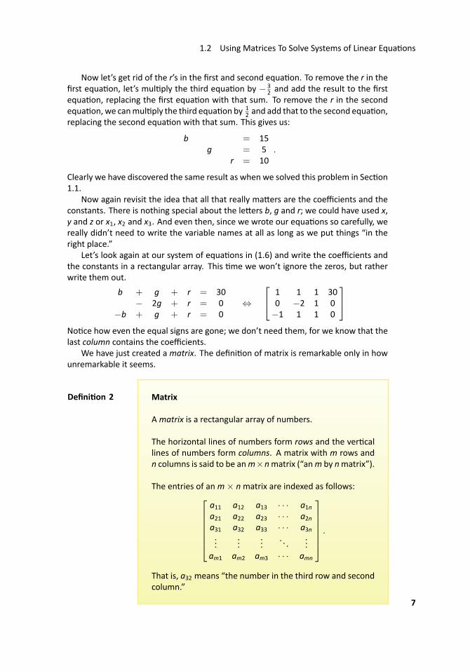
Let’s look again at our system of equa ons in (1.6) and write the coefficients andthe constants in a rectangular array. This me we won’t ignore the zeros, but ratherwrite them out.
b + g + r = 30− 2g + r = 0
−b + g + r = 0⇔
1 1 1 300 −2 1 0−1 1 1 0
No ce how even the equal signs are gone; we don’t need them, for we know that thelast column contains the coefficients.
We have just created amatrix. The defini on of matrix is remarkable only in howunremarkable it seems.
..Defini on 2
.
.Matrix
Amatrix is a rectangular array of numbers.
The horizontal lines of numbers form rows and the ver callines of numbers form columns. A matrix with m rows andn columns is said to be anm×nmatrix (“anm by nmatrix”).
The entries of anm× nmatrix are indexed as follows:a11 a12 a13 · · · a1na21 a22 a23 · · · a2na31 a32 a33 · · · a3n...
......
. . ....
am1 am2 am3 · · · amn
.
That is, a32 means “the number in the third row and secondcolumn.”
7
Chapter 1 Systems of Linear Equa ons
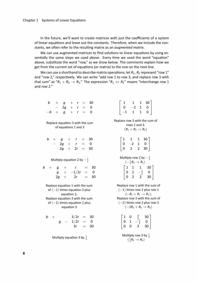
In the future, we’ll want to create matrices with just the coefficients of a systemof linear equa ons and leave out the constants. Therefore, when we include the con-stants, we o en refer to the resul ng matrix as an augmented matrix.
We can use augmented matrices to find solu ons to linear equa ons by using es-sen ally the same steps we used above. Every me we used the word “equa on”above, subs tute the word “row,” as we show below. The comments explain how weget from the current set of equa ons (or matrix) to the one on the next line.
We can use a shorthand to describematrix opera ons; let R1, R2 represent “row 1”and “row 2,” respec vely. We can write “add row 1 to row 3, and replace row 3 withthat sum” as “R1 + R3 → R3.” The expression “R1 ↔ R2” means “interchange row 1and row 2.”
b + g + r = 30− 2g + r = 0
−b + g + r = 0
1 1 1 300 −2 1 0−1 1 1 0
Replace equa on 3 with the sum
of equa ons 1 and 3
Replace row 3 with the sum ofrows 1 and 3.
(R1 + R3 → R3)
b + g + r = 30− 2g + r = 0
2g + 2r = 30
1 1 1 300 −2 1 00 2 2 30
Mul ply equa on 2 by− 1
2Mul ply row 2 by− 1
2(− 1
2R2 → R2)
b + g + r = 30g + −1/2r = 02g + 2r = 30
1 1 1 300 1 − 1
2 00 2 2 30
Replace equa on 1 with the sumof (−1) mes equa on 2 plus
equa on 1;Replace equa on 3 with the sumof (−2) mes equa on 2 plus
equa on 3
Replace row 1 with the sum of(−1) mes row 2 plus row 1
(−R2 + R1 → R1);Replace row 3 with the sum of(−2) mes row 2 plus row 3
(−2R2 + R3 → R3)
b + 3/2r = 30g − 1/2r = 0
3r = 30
1 0 32 30
0 1 − 12 0
0 0 3 30
Mul ply equa on 3 by 1
3Mul ply row 3 by 1
3( 13R3 → R3)
8
1.2 Using Matrices To Solve Systems of Linear Equa ons
b + 3/2r = 30g − 1/2r = 0
r = 10
1 0 32 30
0 1 − 12 0
0 0 1 10
Replace equa on 2 with the sum
of 12 mes equa on 3 plus
equa on 2;Replace equa on 1 with the sumof− 3
2 mes equa on 3 plusequa on 1
Replace row 2 with the sum of 12
mes row 3 plus row 2( 12R3 + R2 → R2);
Replace row 1 with the sum of− 3
2 mes row 3 plus row 1(− 3
2R3 + R1 → R1)
b = 15g = 5
r = 10
1 0 0 150 1 0 50 0 1 10
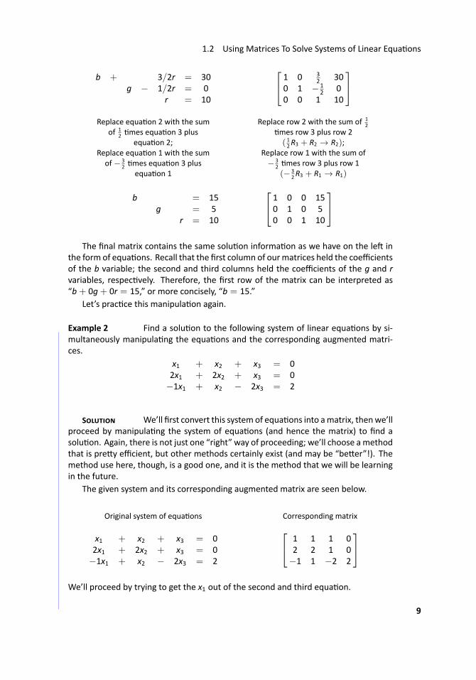
The final matrix contains the same solu on informa on as we have on the le in
the form of equa ons. Recall that the first column of ourmatrices held the coefficientsof the b variable; the second and third columns held the coefficients of the g and rvariables, respec vely. Therefore, the first row of the matrix can be interpreted as“b+ 0g+ 0r = 15,” or more concisely, “b = 15.”
Let’s prac ce this manipula on again.
.. Example 2 ..Find a solu on to the following system of linear equa ons by si-multaneously manipula ng the equa ons and the corresponding augmented matri-ces.
x1 + x2 + x3 = 02x1 + 2x2 + x3 = 0−1x1 + x2 − 2x3 = 2
S We’ll first convert this systemof equa ons into amatrix, thenwe’llproceed by manipula ng the system of equa ons (and hence the matrix) to find asolu on. Again, there is not just one “right” way of proceeding; we’ll choose amethodthat is pre y efficient, but other methods certainly exist (and may be “be er”!). Themethod use here, though, is a good one, and it is the method that we will be learningin the future.
The given system and its corresponding augmented matrix are seen below.
Original system of equa ons Corresponding matrix
x1 + x2 + x3 = 02x1 + 2x2 + x3 = 0−1x1 + x2 − 2x3 = 2
1 1 1 02 2 1 0−1 1 −2 2
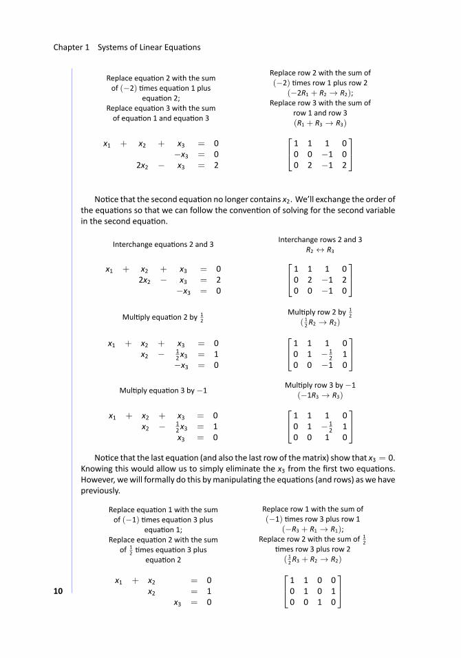
We’ll proceed by trying to get the x1 out of the second and third equa on.
9
Chapter 1 Systems of Linear Equa ons
Replace equa on 2 with the sumof (−2) mes equa on 1 plus
equa on 2;Replace equa on 3 with the sumof equa on 1 and equa on 3
Replace row 2 with the sum of(−2) mes row 1 plus row 2
(−2R1 + R2 → R2);Replace row 3 with the sum of
row 1 and row 3(R1 + R3 → R3)
x1 + x2 + x3 = 0−x3 = 0
2x2 − x3 = 2
1 1 1 00 0 −1 00 2 −1 2
..No ce that the second equa on no longer contains x2. We’ll exchange the order of
the equa ons so that we can follow the conven on of solving for the second variablein the second equa on.
Interchange equa ons 2 and 3Interchange rows 2 and 3
R2 ↔ R3
x1 + x2 + x3 = 02x2 − x3 = 2
−x3 = 0
1 1 1 00 2 −1 20 0 −1 0
Mul ply equa on 2 by 1
2Mul ply row 2 by 1
2( 12R2 → R2)
x1 + x2 + x3 = 0x2 − 1
2x3 = 1−x3 = 0
1 1 1 00 1 − 1
2 10 0 −1 0
Mul ply equa on 3 by−1
Mul ply row 3 by−1(−1R3 → R3)
x1 + x2 + x3 = 0x2 − 1
2x3 = 1x3 = 0
1 1 1 00 1 − 1
2 10 0 1 0
No ce that the last equa on (and also the last row of thematrix) show that x3 = 0.
Knowing this would allow us to simply eliminate the x3 from the first two equa ons.However, wewill formally do this bymanipula ng the equa ons (and rows) as we havepreviously.
Replace equa on 1 with the sumof (−1) mes equa on 3 plus
equa on 1;Replace equa on 2 with the sum
of 12 mes equa on 3 plus
equa on 2
Replace row 1 with the sum of(−1) mes row 3 plus row 1
(−R3 + R1 → R1);Replace row 2 with the sum of 1
2mes row 3 plus row 2( 12R3 + R2 → R2)
x1 + x2 = 0x2 = 1
x3 = 0
1 1 0 00 1 0 10 0 1 0
10
1.2 Using Matrices To Solve Systems of Linear Equa ons
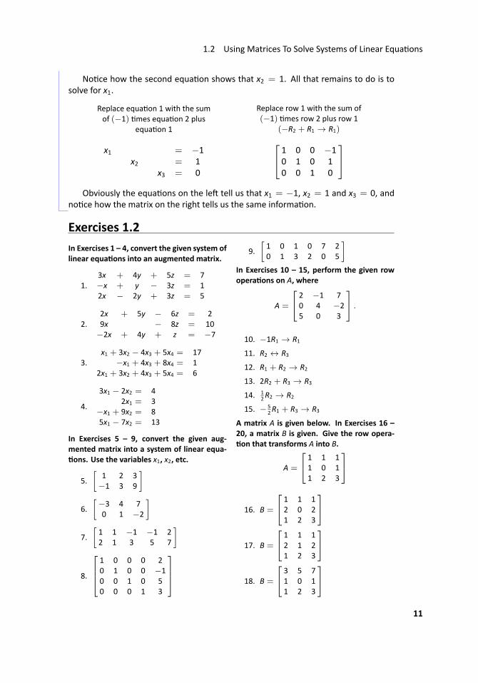
No ce how the second equa on shows that x2 = 1. All that remains to do is tosolve for x1.
Replace equa on 1 with the sumof (−1) mes equa on 2 plus
equa on 1
Replace row 1 with the sum of(−1) mes row 2 plus row 1
(−R2 + R1 → R1)
x1 = −1x2 = 1
x3 = 0
1 0 0 −10 1 0 10 0 1 0
Obviously the equa ons on the le tell us that x1 = −1, x2 = 1 and x3 = 0, and
no ce how the matrix on the right tells us the same informa on. ...
Exercises 1.2In Exercises 1 – 4, convert the given system oflinear equa ons into an augmented matrix.
1.3x + 4y + 5z = 7−x + y − 3z = 12x − 2y + 3z = 5
2.2x + 5y − 6z = 29x − 8z = 10−2x + 4y + z = −7
3.x1 + 3x2 − 4x3 + 5x4 = 17
−x1 + 4x3 + 8x4 = 12x1 + 3x2 + 4x3 + 5x4 = 6
4.
3x1 − 2x2 = 42x1 = 3
−x1 + 9x2 = 85x1 − 7x2 = 13
In Exercises 5 – 9, convert the given aug-mented matrix into a system of linear equa-ons. Use the variables x1, x2, etc.
5.[
1 2 3−1 3 9
]
6.[−3 4 70 1 −2
]
7.[1 1 −1 −1 22 1 3 5 7
]
8.
1 0 0 0 20 1 0 0 −10 0 1 0 50 0 0 1 3
9.[1 0 1 0 7 20 1 3 2 0 5
]In Exercises 10 – 15, perform the given rowopera ons on A, where
A =
2 −1 70 4 −25 0 3
.
10. −1R1 → R1
11. R2 ↔ R3
12. R1 + R2 → R2
13. 2R2 + R3 → R3
14. 12R2 → R2
15. − 52R1 + R3 → R3
A matrix A is given below. In Exercises 16 –20, a matrix B is given. Give the row opera-on that transforms A into B.
A =
1 1 11 0 11 2 3
16. B =
1 1 12 0 21 2 3
17. B =
1 1 12 1 21 2 3
18. B =
3 5 71 0 11 2 3
11
Chapter 1 Systems of Linear Equa ons
19. B =
1 0 11 1 11 2 3
20. B =
1 1 11 0 10 2 2
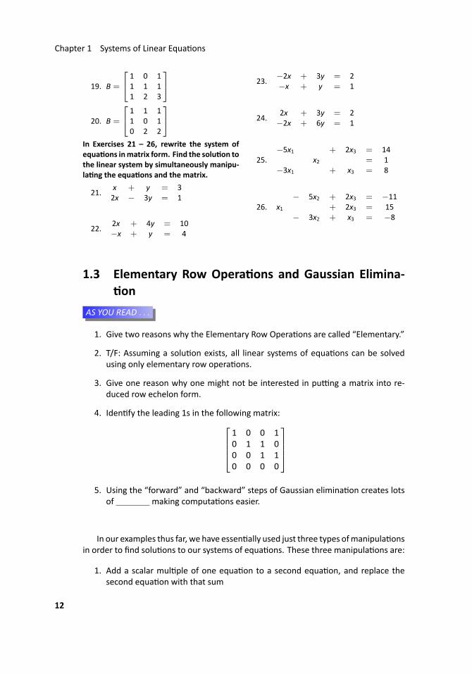
In Exercises 21 – 26, rewrite the system ofequa ons inmatrix form. Find the solu on tothe linear system by simultaneously manipu-la ng the equa ons and the matrix.
21.x + y = 32x − 3y = 1
22.2x + 4y = 10−x + y = 4
23.−2x + 3y = 2−x + y = 1
24.2x + 3y = 2−2x + 6y = 1
25.−5x1 + 2x3 = 14
x2 = 1−3x1 + x3 = 8
26.− 5x2 + 2x3 = −11
x1 + 2x3 = 15− 3x2 + x3 = −8
1.3 Elementary Row Opera ons and Gaussian Elimina-on...AS YOU READ . . .
1. Give two reasons why the Elementary Row Opera ons are called “Elementary.”
2. T/F: Assuming a solu on exists, all linear systems of equa ons can be solvedusing only elementary row opera ons.
3. Give one reason why one might not be interested in pu ng a matrix into re-duced row echelon form.
4. Iden fy the leading 1s in the following matrix:1 0 0 10 1 1 00 0 1 10 0 0 0
5. Using the “forward” and “backward” steps of Gaussian elimina on creates lots
of making computa ons easier.
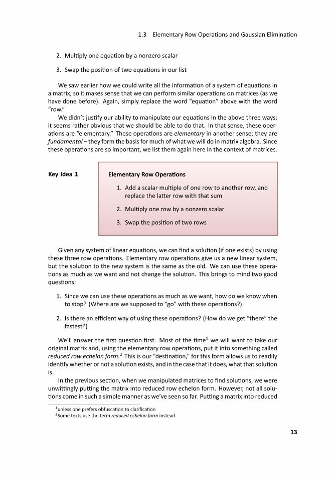
In our examples thus far, we have essen ally used just three types ofmanipula onsin order to find solu ons to our systems of equa ons. These three manipula ons are:
1. Add a scalar mul ple of one equa on to a second equa on, and replace thesecond equa on with that sum
12
1.3 Elementary Row Opera ons and Gaussian Elimina on
2. Mul ply one equa on by a nonzero scalar
3. Swap the posi on of two equa ons in our list
We saw earlier how we could write all the informa on of a system of equa ons ina matrix, so it makes sense that we can perform similar opera ons on matrices (as wehave done before). Again, simply replace the word “equa on” above with the word“row.”
We didn’t jus fy our ability to manipulate our equa ons in the above three ways;it seems rather obvious that we should be able to do that. In that sense, these oper-a ons are “elementary.” These opera ons are elementary in another sense; they arefundamental – they form the basis formuch of what wewill do inmatrix algebra. Sincethese opera ons are so important, we list them again here in the context of matrices.
..Key Idea 1
.
.Elementary Row Opera ons
1. Add a scalar mul ple of one row to another row, andreplace the la er row with that sum
2. Mul ply one row by a nonzero scalar
3. Swap the posi on of two rows
Given any system of linear equa ons, we can find a solu on (if one exists) by usingthese three row opera ons. Elementary row opera ons give us a new linear system,but the solu on to the new system is the same as the old. We can use these opera-ons as much as we want and not change the solu on. This brings to mind two good
ques ons:
1. Since we can use these opera ons as much as we want, how do we know whento stop? (Where are we supposed to “go” with these opera ons?)
2. Is there an efficient way of using these opera ons? (How do we get “there” thefastest?)
We’ll answer the first ques on first. Most of the me1 we will want to take ouroriginal matrix and, using the elementary row opera ons, put it into something calledreduced row echelon form.2 This is our “des na on,” for this form allows us to readilyiden fywhether or not a solu on exists, and in the case that it does, what that solu onis.
In the previous sec on, when we manipulated matrices to find solu ons, we wereunwi ngly pu ng the matrix into reduced row echelon form. However, not all solu-ons come in such a simplemanner as we’ve seen so far. Pu ng amatrix into reduced
1unless one prefers obfusca on to clarifica on2Some texts use the term reduced echelon form instead.
13
Chapter 1 Systems of Linear Equa ons
row echelon form helps us iden fy all types of solu ons. We’ll explore the topic of un-derstanding what the reduced row echelon form of a matrix tells us in the followingsec ons; in this sec on we focus on finding it.
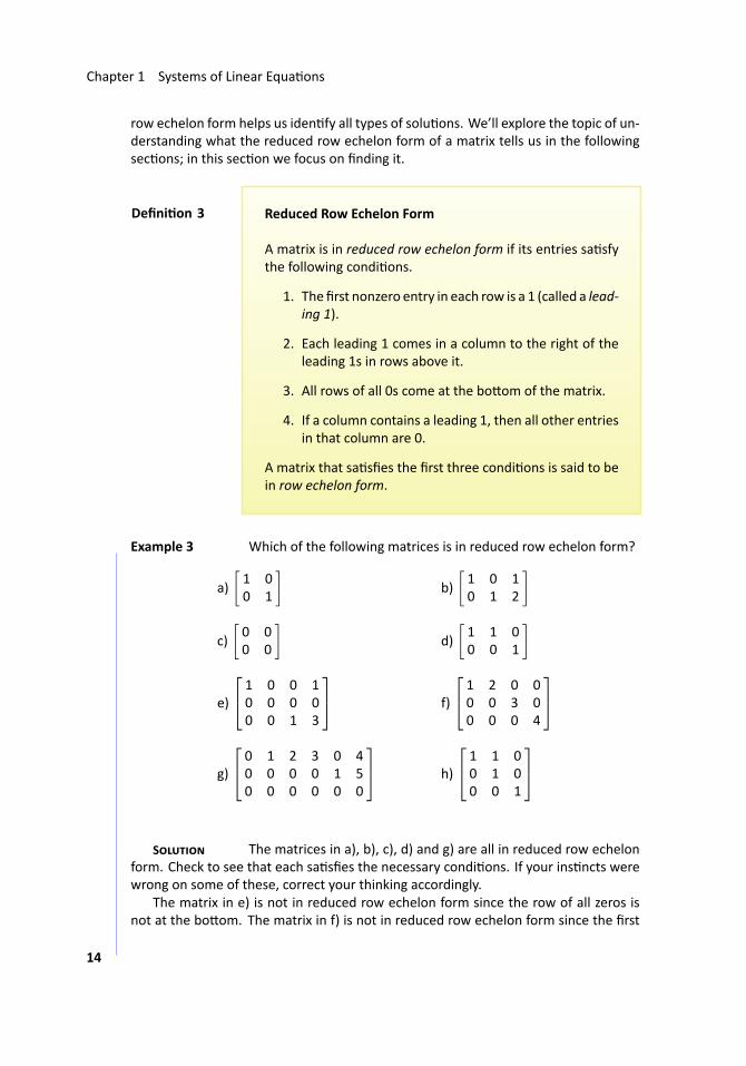
..Defini on 3
.
.Reduced Row Echelon Form
A matrix is in reduced row echelon form if its entries sa sfythe following condi ons.
1. The first nonzero entry in each row is a 1 (called a lead-ing 1).
2. Each leading 1 comes in a column to the right of theleading 1s in rows above it.
3. All rows of all 0s come at the bo om of the matrix.
4. If a column contains a leading 1, then all other entriesin that column are 0.
A matrix that sa sfies the first three condi ons is said to bein row echelon form.
.. Example 3 ..Which of the following matrices is in reduced row echelon form?
a)[1 00 1
]b)
[1 0 10 1 2
]
c)[0 00 0
]d)
[1 1 00 0 1
]
e)
1 0 0 10 0 0 00 0 1 3
f)
1 2 0 00 0 3 00 0 0 4
g)
0 1 2 3 0 40 0 0 0 1 50 0 0 0 0 0
h)
1 1 00 1 00 0 1
S The matrices in a), b), c), d) and g) are all in reduced row echelonform. Check to see that each sa sfies the necessary condi ons. If your ins ncts werewrong on some of these, correct your thinking accordingly.
The matrix in e) is not in reduced row echelon form since the row of all zeros isnot at the bo om. The matrix in f) is not in reduced row echelon form since the first
14
1.3 Elementary Row Opera ons and Gaussian Elimina on
nonzero entries in rows 2 and 3 are not 1. Finally, the matrix in h) is not in reducedrow echelon form since the first entry in column 2 is not zero; the second 1 in column2 is a leading one, hence all other entries in that column should be 0.
We end this example with a preview of what we’ll learn in the future. Considerthe matrix in b). If this matrix came from the augmented matrix of a system of linearequa ons, then we can readily recognize that the solu on of the system is x1 = 1 andx2 = 2. Again, in previous examples, when we found the solu on to a linear system,we were unwi ngly pu ng our matrices into reduced row echelon form. ...
We began this sec on discussing how we can manipulate the entries in a matrixwith elementary row opera ons. This led to two ques ons, “Where do we go?” and“How do we get there quickly?” We’ve just answered the first ques on: most of theme we are “going to” reduced row echelon form. We now address the second ques-on.There is no one “right” way of using these opera ons to transform a matrix into
reduced row echelon form. However, there is a general technique that works very wellin that it is very efficient (sowe don’twaste meon unnecessary steps). This techniqueis called Gaussian elimina on. It is named in honor of the great mathema cian KarlFriedrich Gauss.
While this technique isn’t very difficult to use, it is one of those things that is eas-ier understood by watching it being used than explained as a series of steps. With thisin mind, we will go through one more example highligh ng important steps and thenwe’ll explain the procedure in detail.
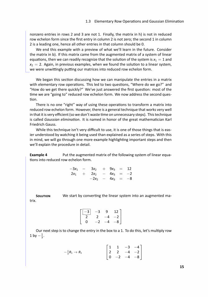
.. Example 4 ..Put the augmented matrix of the following system of linear equa-ons into reduced row echelon form.
−3x1 − 3x2 + 9x3 = 122x1 + 2x2 − 4x3 = −2
−2x2 − 4x3 = −8
S We start by conver ng the linear system into an augmented ma-trix. −3 −3 9 12
2 2 −4 −20 −2 −4 −8
Our next step is to change the entry in the box to a 1. To do this, let’s mul ply row
1 by− 13 .
− 13R1 → R1
1 1 −3 −42 2 −4 −20 −2 −4 −8
15
Chapter 1 Systems of Linear Equa ons
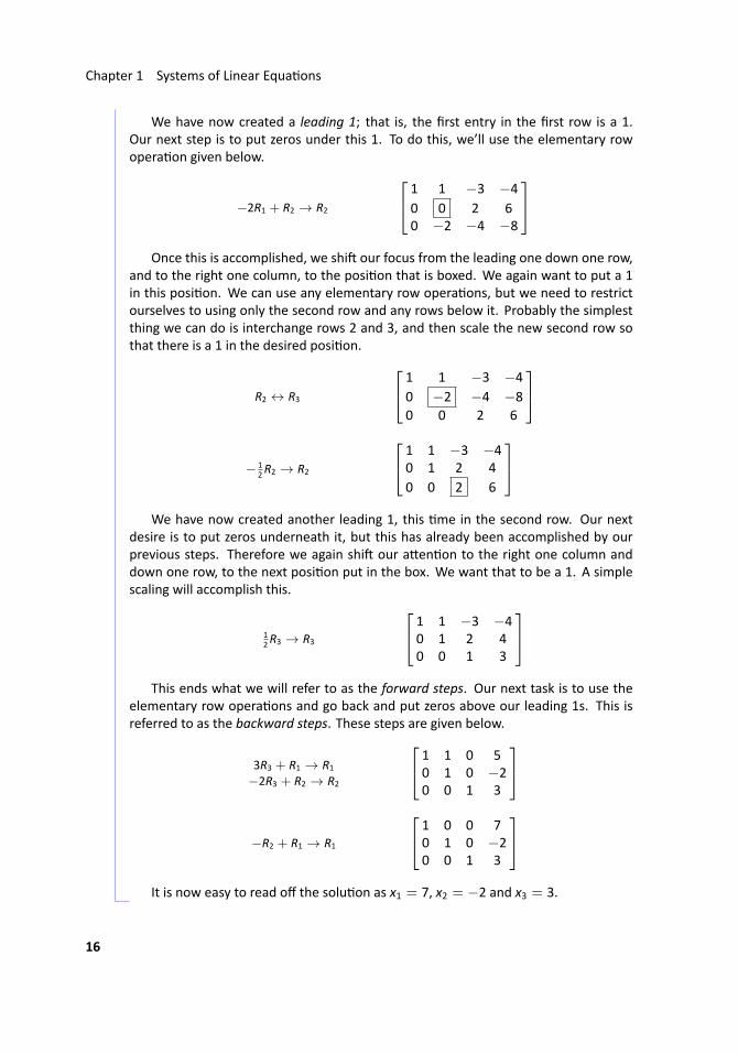
We have now created a leading 1; that is, the first entry in the first row is a 1.Our next step is to put zeros under this 1. To do this, we’ll use the elementary rowopera on given below.
−2R1 + R2 → R2
1 1 −3 −40 0 2 60 −2 −4 −8
Once this is accomplished, we shi our focus from the leading one down one row,
and to the right one column, to the posi on that is boxed. We again want to put a 1in this posi on. We can use any elementary row opera ons, but we need to restrictourselves to using only the second row and any rows below it. Probably the simplestthing we can do is interchange rows 2 and 3, and then scale the new second row sothat there is a 1 in the desired posi on.
R2 ↔ R3
1 1 −3 −40 −2 −4 −80 0 2 6
− 12R2 → R2
1 1 −3 −40 1 2 40 0 2 6
We have now created another leading 1, this me in the second row. Our next
desire is to put zeros underneath it, but this has already been accomplished by ourprevious steps. Therefore we again shi our a en on to the right one column anddown one row, to the next posi on put in the box. We want that to be a 1. A simplescaling will accomplish this.
12R3 → R3
1 1 −3 −40 1 2 40 0 1 3
This ends what we will refer to as the forward steps. Our next task is to use the
elementary row opera ons and go back and put zeros above our leading 1s. This isreferred to as the backward steps. These steps are given below.
3R3 + R1 → R1
−2R3 + R2 → R2
1 1 0 50 1 0 −20 0 1 3
−R2 + R1 → R1
1 0 0 70 1 0 −20 0 1 3
It is now easy to read off the solu on as x1 = 7, x2 = −2 and x3 = 3. ...
16
1.3 Elementary Row Opera ons and Gaussian Elimina on
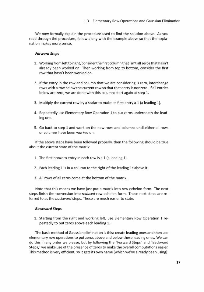
We now formally explain the procedure used to find the solu on above. As youread through the procedure, follow along with the example above so that the expla-na on makes more sense.
Forward Steps
1. Working from le to right, consider the first column that isn’t all zeros that hasn’talready been worked on. Then working from top to bo om, consider the firstrow that hasn’t been worked on.
2. If the entry in the row and column that we are considering is zero, interchangerowswith a row below the current row so that that entry is nonzero. If all entriesbelow are zero, we are done with this column; start again at step 1.
3. Mul ply the current row by a scalar to make its first entry a 1 (a leading 1).
4. Repeatedly use Elementary Row Opera on 1 to put zeros underneath the lead-ing one.
5. Go back to step 1 and work on the new rows and columns un l either all rowsor columns have been worked on.
If the above steps have been followed properly, then the following should be trueabout the current state of the matrix:
1. The first nonzero entry in each row is a 1 (a leading 1).
2. Each leading 1 is in a column to the right of the leading 1s above it.
3. All rows of all zeros come at the bo om of the matrix.
Note that this means we have just put a matrix into row echelon form. The nextsteps finish the conversion into reduced row echelon form. These next steps are re-ferred to as the backward steps. These are much easier to state.
Backward Steps
1. Star ng from the right and working le , use Elementary Row Opera on 1 re-peatedly to put zeros above each leading 1.
The basic method of Gaussian elimina on is this: create leading ones and then useelementary row opera ons to put zeros above and below these leading ones. We cando this in any order we please, but by following the “Forward Steps” and “BackwardSteps,” wemake use of the presence of zeros to make the overall computa ons easier.This method is very efficient, so it gets its own name (which we’ve already been using).
17
Chapter 1 Systems of Linear Equa ons
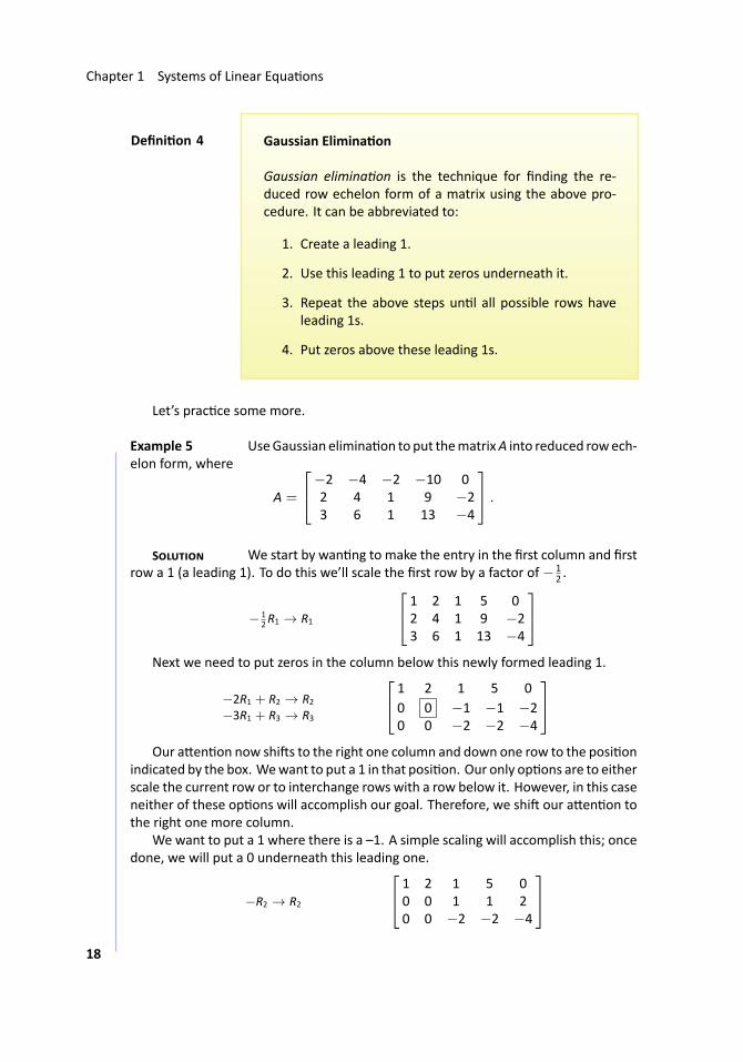
..Defini on 4
.
.Gaussian Elimina on
Gaussian elimina on is the technique for finding the re-duced row echelon form of a matrix using the above pro-cedure. It can be abbreviated to:
1. Create a leading 1.
2. Use this leading 1 to put zeros underneath it.
3. Repeat the above steps un l all possible rows haveleading 1s.
4. Put zeros above these leading 1s.
Let’s prac ce some more.
.. Example 5 ..UseGaussian elimina on to put thematrixA into reduced rowech-elon form, where
A =
−2 −4 −2 −10 02 4 1 9 −23 6 1 13 −4
.
S We start by wan ng to make the entry in the first column and firstrow a 1 (a leading 1). To do this we’ll scale the first row by a factor of− 1
2 .
− 12R1 → R1
1 2 1 5 02 4 1 9 −23 6 1 13 −4
Next we need to put zeros in the column below this newly formed leading 1.
−2R1 + R2 → R2
−3R1 + R3 → R3
1 2 1 5 00 0 −1 −1 −20 0 −2 −2 −4
Our a en on now shi s to the right one column and down one row to the posi on
indicated by the box. Wewant to put a 1 in that posi on. Our only op ons are to eitherscale the current row or to interchange rows with a row below it. However, in this caseneither of these op ons will accomplish our goal. Therefore, we shi our a en on tothe right one more column.
We want to put a 1 where there is a –1. A simple scaling will accomplish this; oncedone, we will put a 0 underneath this leading one.
−R2 → R2
1 2 1 5 00 0 1 1 20 0 −2 −2 −4
18
1.3 Elementary Row Opera ons and Gaussian Elimina on
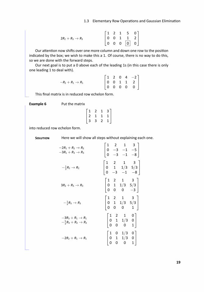
2R2 + R3 → R3
1 2 1 5 00 0 1 1 20 0 0 0 0
Our a en on now shi s over one more column and down one row to the posi on
indicated by the box; we wish to make this a 1. Of course, there is no way to do this,so we are done with the forward steps.
Our next goal is to put a 0 above each of the leading 1s (in this case there is onlyone leading 1 to deal with).
−R2 + R1 → R1
1 2 0 4 −20 0 1 1 20 0 0 0 0
This final matrix is in reduced row echelon form. ...
.. Example 6 Put the matrix 1 2 1 32 1 1 13 3 2 1
into reduced row echelon form.
S Here we will show all steps without explaining each one.
−2R1 + R2 → R2
−3R1 + R3 → R3
1 2 1 30 −3 −1 −50 −3 −1 −8
− 1
3R2 → R2
1 2 1 30 1 1/3 5/30 −3 −1 −8
3R2 + R3 → R3
1 2 1 30 1 1/3 5/30 0 0 −3
− 1
3R3 → R3
1 2 1 30 1 1/3 5/30 0 0 1
−3R3 + R1 → R1
− 53R3 + R2 → R2
1 2 1 00 1 1/3 00 0 0 1
−2R2 + R1 → R1
1 0 1/3 00 1 1/3 00 0 0 1
..
19
Chapter 1 Systems of Linear Equa ons
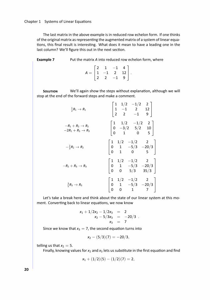
The last matrix in the above example is in reduced row echelon form. If one thinksof the original matrix as represen ng the augmentedmatrix of a system of linear equa-ons, this final result is interes ng. What does it mean to have a leading one in the
last column? We’ll figure this out in the next sec on.
.. Example 7 ..Put the matrix A into reduced row echelon form, where
A =
2 1 −1 41 −1 2 122 2 −1 9
.
S We’ll again show the steps without explana on, although we willstop at the end of the forward steps and make a comment.
12R1 → R1
1 1/2 −1/2 21 −1 2 122 2 −1 9
−R1 + R2 → R2
−2R1 + R3 → R3
1 1/2 −1/2 20 −3/2 5/2 100 1 0 5
− 23R2 → R2
1 1/2 −1/2 20 1 −5/3 −20/30 1 0 5
−R2 + R3 → R3
1 1/2 −1/2 20 1 −5/3 −20/30 0 5/3 35/3
35R3 → R3
1 1/2 −1/2 20 1 −5/3 −20/30 0 1 7
Let’s take a break here and think about the state of our linear system at this mo-
ment. Conver ng back to linear equa ons, we now know
x1 + 1/2x2 − 1/2x3 = 2x2 − 5/3x3 = −20/3
x3 = 7.
Since we know that x3 = 7, the second equa on turns into
x2 − (5/3)(7) = −20/3,
telling us that x2 = 5.Finally, knowing values for x2 and x3 lets us subs tute in the first equa on and find
x1 + (1/2)(5)− (1/2)(7) = 2,
20
1.3 Elementary Row Opera ons and Gaussian Elimina on
so x1 = 3.
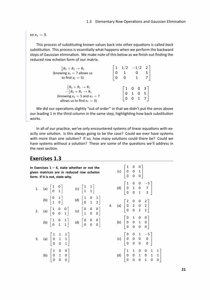
This process of subs tu ng known values back into other equa ons is called backsubs tu on. This process is essen ally what happens when we perform the backwardsteps of Gaussian elimina on. Wemake note of this below as we finish out finding thereduced row echelon form of our matrix.
53R3 + R2 → R2
(knowing x3 = 7 allows usto find x2 = 5)
1 1/2 −1/2 20 1 0 50 0 1 7
12R3 + R1 → R1
− 12R2 + R1 → R1
(knowing x2 = 5 and x3 = 7allows us to find x1 = 3)
1 0 0 30 1 0 50 0 1 7
We did our opera ons slightly “out of order” in that we didn’t put the zeros above
our leading 1 in the third column in the same step, highligh ng how back subs tu onworks. ...
In all of our prac ce, we’ve only encountered systems of linear equa ons with ex-actly one solu on. Is this always going to be the case? Could we ever have systemswith more than one solu on? If so, how many solu ons could there be? Could wehave systems without a solu on? These are some of the ques ons we’ll address inthe next sec on.
Exercises 1.3In Exercises 1 – 4, state whether or not thegiven matrices are in reduced row echelonform. If it is not, state why.
1. (a)[1 00 1
](b)
[0 11 0
] (c)[1 11 1
](d)
[1 0 10 1 2
]2. (a)
[1 0 00 0 1
](b)
[1 0 10 1 1
] (c)[0 0 01 0 0
](d)
[0 0 00 0 0
]
3. (a)
1 1 10 1 10 0 1
(b)
1 0 00 1 00 0 0
(c)
1 0 00 0 10 0 0
(d)
1 0 0 −50 1 0 70 0 1 3
4. (a)
2 0 0 20 2 0 20 0 2 2
(b)
0 1 0 00 0 1 00 0 0 0
(c)
0 0 1 −50 0 0 00 0 0 0
(d)
1 1 0 0 1 10 0 1 0 1 10 0 0 1 0 0
21
Chapter 1 Systems of Linear Equa ons
In Exercises 5 – 22, use Gaussian Elimina onto put the given matrix into reduced row ech-elon form.
5.[
1 2−3 −5
]6.
[2 −23 −2
]7.
[4 12−2 −6
]8.
[−5 710 14
]9.
[−1 1 4−2 1 1
]10.
[7 2 33 1 2
]11.
[3 −3 6−1 1 −2
]12.
[4 5 −6
−12 −15 18
]
13.
−2 −4 −8−2 −3 −52 3 6
14.
2 1 11 1 12 1 2
15.
1 2 11 3 1−1 −3 0
16.
1 2 30 4 51 6 9
17.
1 1 1 22 −1 −1 1−1 1 1 0
18.
2 −1 1 53 1 6 −13 0 5 0
19.
1 1 −1 72 1 0 103 2 −1 17
20.
4 1 8 151 1 2 73 1 5 11
21.
[2 2 1 3 1 41 1 1 3 1 4
]
22.[1 −1 3 1 −2 92 −2 6 1 −2 13
]
1.4 Existence and Uniqueness of Solu ons
...AS YOU READ . . .
1. T/F: It is possible for a linear system to have exactly 5 solu ons.
2. T/F: A variable that corresponds to a leading 1 is “free.”
3. How can one tell what kind of solu on a linear system of equa ons has?
4. Give an example (different from those given in the text) of a 2 equa on, 2 un-known linear system that is not consistent.
5. T/F: A par cular solu on for a linear system with infinite solu ons can be foundby arbitrarily picking values for the free variables.
22
1.4 Existence and Uniqueness of Solu ons
So far, whenever we have solved a system of linear equa ons, we have alwaysfound exactly one solu on. This is not always the case; we will find in this sec on thatsome systems do not have a solu on, and others have more than one.
We start with a very simple example. Consider the following linear system:
x− y = 0.
There are obviously infinite solu ons to this system; as long as x = y, we have a so-lu on. We can picture all of these solu ons by thinking of the graph of the equa ony = x on the tradi onal x, y coordinate plane.
Let’s con nue this visual aspect of considering solu ons to linear systems. Con-sider the system
x+ y = 2
x− y = 0.
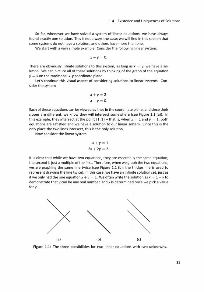
Each of these equa ons can be viewed as lines in the coordinate plane, and since theirslopes are different, we know they will intersect somewhere (see Figure 1.1 (a)). Inthis example, they intersect at the point (1, 1) – that is, when x = 1 and y = 1, bothequa ons are sa sfied and we have a solu on to our linear system. Since this is theonly place the two lines intersect, this is the only solu on.
Now consider the linear system
x+ y = 1
2x+ 2y = 2.
It is clear that while we have two equa ons, they are essen ally the same equa on;the second is just a mul ple of the first. Therefore, when we graph the two equa ons,we are graphing the same line twice (see Figure 1.1 (b); the thicker line is used torepresent drawing the line twice). In this case, we have an infinite solu on set, just asif we only had the one equa on x+ y = 1. We o en write the solu on as x = 1− y todemonstrate that y can be any real number, and x is determined once we pick a valuefor y.
..
(a)
.
(b)
.
(c)
..Figure 1.1: The three possibili es for two linear equa ons with two unknowns.
23
Chapter 1 Systems of Linear Equa ons
Finally, consider the linear system
x+ y = 1
x+ y = 2.
We should immediately spot a problem with this system; if the sum of x and y is 1,how can it also be 2? There is no solu on to such a problem; this linear system has nosolu on. We can visualize this situa on in Figure 1.1 (c); the two lines are parallel andnever intersect.
If wewere to consider a linear systemwith three equa ons and two unknowns, wecould visualize the solu on by graphing the corresponding three lines. We can picturethat perhaps all three lines would meet at one point, giving exactly 1 solu on; per-haps all three equa ons describe the same line, giving an infinite number of solu ons;perhaps we have different lines, but they do not all meet at the same point, givingno solu on. We further visualize similar situa ons with, say, 20 equa ons with twovariables.
While it becomes harder to visualize when we add variables, no ma er how manyequa ons and variables we have, solu ons to linear equa ons always come in one ofthree forms: exactly one solu on, infinite solu ons, or no solu on. This is a fact thatwe will not prove here, but it deserves to be stated.
..Theorem 1
.
.Solu on Forms of Linear Systems
Every linear system of equa ons has exactly one solu on,infinite solu ons, or no solu on.
This leads us to a defini on. Here we don’t differen ate between having one so-lu on and infinite solu ons, but rather just whether or not a solu on exists.
..Defini on 5
.
.Consistent and Inconsistent Linear Systems
A system of linear equa ons is consistent if it has a solu on(perhaps more than one). A linear system is inconsistent ifit does not have a solu on.
How can we tell what kind of solu on (if one exists) a given system of linear equa-ons has? The answer to this ques on lies with properly understanding the reduced
row echelon form of a matrix. To discover what the solu on is to a linear system, wefirst put the matrix into reduced row echelon form and then interpret that form prop-erly.
Before we start with a simple example, let us make a note about finding the re-
24
1.4 Existence and Uniqueness of Solu ons
duced row echelon form of a matrix.
TechnologyNote: In the previous sec on, we learned how to find the reduced rowechelon form of a matrix using Gaussian elimina on – by hand. We need to know howto do this; understanding the process has benefits. However, actually execu ng theprocess by hand for every problem is not usually beneficial. In fact, with large systems,compu ng the reduced row echelon form by hand is effec vely impossible. Our mainconcern iswhat “the rref” is, notwhat exact stepswere used to arrive there. Therefore,the reader is encouraged to employ some form of technology to find the reduced rowechelon form. Computer programs such asMathema ca, MATLAB, Maple, and Derivecan be used; many handheld calculators (such as Texas Instruments calculators) willperform these calcula ons very quickly.
As a general rule, when we are learning a new technique, it is best to not usetechnology to aid us. This helps us learn not only the technique but some of its “innerworkings.” We can then use technology once we havemastered the technique and arenow learning how to use it to solve problems.
From here on out, in our examples, when we need the reduced row echelon formof a matrix, we will not show the steps involved. Rather, we will give the ini al matrix,then immediately give the reduced row echelon form of the matrix. We trust that thereader can verify the accuracy of this form by both performing the necessary steps byhand or u lizing some technology to do it for them.
Our first example explores officially a quick example used in the introduc on ofthis sec on.
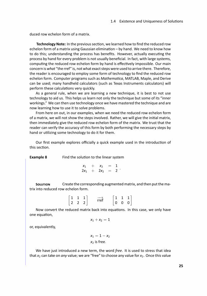
.. Example 8 ..Find the solu on to the linear system
x1 + x2 = 12x1 + 2x2 = 2
.
S Create the corresponding augmentedmatrix, and thenput thema-trix into reduced row echelon form.[
1 1 12 2 2
]−→rref
[1 1 10 0 0
]Now convert the reduced matrix back into equa ons. In this case, we only have
one equa on,x1 + x2 = 1
or, equivalently,
x1 = 1− x2x2 is free.
We have just introduced a new term, the word free. It is used to stress that ideathat x2 can take on any value; we are “free” to choose any value for x2. Once this value
25
Chapter 1 Systems of Linear Equa ons
is chosen, the value of x1 is determined. We have infinite choices for the value of x2,so therefore we have infinite solu ons.
For example, if we set x2 = 0, then x1 = 1; if we set x2 = 5, then x1 = −4. ...
Let’s try another example, one that uses more variables.
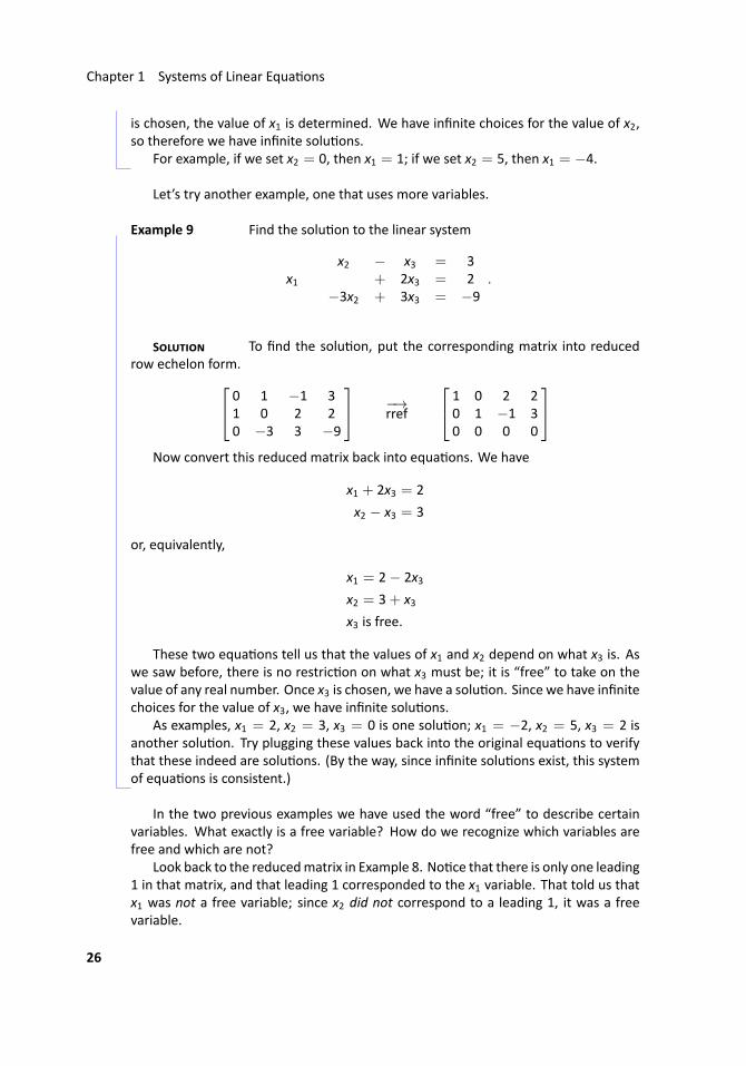
.. Example 9 Find the solu on to the linear system
x2 − x3 = 3x1 + 2x3 = 2
−3x2 + 3x3 = −9.
S To find the solu on, put the corresponding matrix into reducedrow echelon form. 0 1 −1 3
1 0 2 20 −3 3 −9
−→rref
1 0 2 20 1 −1 30 0 0 0
Now convert this reduced matrix back into equa ons. We have
x1 + 2x3 = 2
x2 − x3 = 3
or, equivalently,
x1 = 2− 2x3x2 = 3+ x3x3 is free.
These two equa ons tell us that the values of x1 and x2 depend on what x3 is. Aswe saw before, there is no restric on on what x3 must be; it is “free” to take on thevalue of any real number. Once x3 is chosen, we have a solu on. Since we have infinitechoices for the value of x3, we have infinite solu ons.
As examples, x1 = 2, x2 = 3, x3 = 0 is one solu on; x1 = −2, x2 = 5, x3 = 2 isanother solu on. Try plugging these values back into the original equa ons to verifythat these indeed are solu ons. (By the way, since infinite solu ons exist, this systemof equa ons is consistent.) ..
In the two previous examples we have used the word “free” to describe certainvariables. What exactly is a free variable? How do we recognize which variables arefree and which are not?
Look back to the reducedmatrix in Example 8. No ce that there is only one leading1 in that matrix, and that leading 1 corresponded to the x1 variable. That told us thatx1 was not a free variable; since x2 did not correspond to a leading 1, it was a freevariable.
26
1.4 Existence and Uniqueness of Solu ons
Look also at the reduced matrix in Example 9. There were two leading 1s in thatmatrix; one corresponded to x1 and the other to x2. This meant that x1 and x2 werenot free variables; since there was not a leading 1 that corresponded to x3, it was afree variable.
We formally define this and a few other terms in this following defini on.
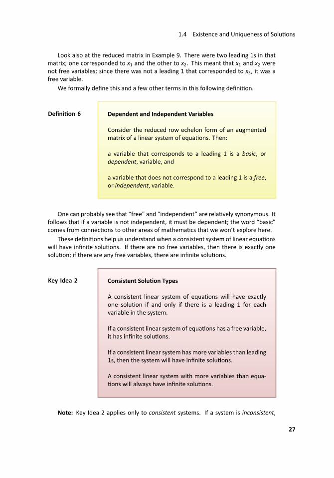
..Defini on 6
.
.Dependent and Independent Variables
Consider the reduced row echelon form of an augmentedmatrix of a linear system of equa ons. Then:
a variable that corresponds to a leading 1 is a basic, ordependent, variable, and
a variable that does not correspond to a leading 1 is a free,or independent, variable.
One can probably see that “free” and “independent” are rela vely synonymous. Itfollows that if a variable is not independent, it must be dependent; the word “basic”comes from connec ons to other areas of mathema cs that we won’t explore here.
These defini ons help us understand when a consistent system of linear equa onswill have infinite solu ons. If there are no free variables, then there is exactly onesolu on; if there are any free variables, there are infinite solu ons.
..Key Idea 2
.
.Consistent Solu on Types
A consistent linear system of equa ons will have exactlyone solu on if and only if there is a leading 1 for eachvariable in the system.
If a consistent linear system of equa ons has a free variable,it has infinite solu ons.
If a consistent linear system has more variables than leading1s, then the system will have infinite solu ons.
A consistent linear system with more variables than equa-ons will always have infinite solu ons.
Note: Key Idea 2 applies only to consistent systems. If a system is inconsistent,
27
Chapter 1 Systems of Linear Equa ons
then no solu on exists and talking about free and basic variables is meaningless.
When a consistent system has only one solu on, each equa on that comes fromthe reduced row echelon form of the corresponding augmented matrix will containexactly one variable. If the consistent system has infinite solu ons, then there will beat least one equa on coming from the reduced row echelon form that contains morethan one variable. The “first” variable will be the basic (or dependent) variable; allothers will be free variables.
We have now seen examples of consistent systems with exactly one solu on andothers with infinite solu ons. How will we recognize that a system is inconsistent?Let’s find out through an example.
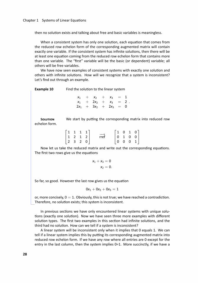
.. Example 10 Find the solu on to the linear system
x1 + x2 + x3 = 1x1 + 2x2 + x3 = 22x1 + 3x2 + 2x3 = 0
.
S We start by pu ng the corresponding matrix into reduced rowechelon form. 1 1 1 1
1 2 1 22 3 2 0
−→rref
1 0 1 00 1 0 00 0 0 1
Now let us take the reduced matrix and write out the corresponding equa ons.
The first two rows give us the equa ons
x1 + x3 = 0
x2 = 0.
So far, so good. However the last row gives us the equa on
0x1 + 0x2 + 0x3 = 1
or, more concisely, 0 = 1. Obviously, this is not true; we have reached a contradic on.Therefore, no solu on exists; this system is inconsistent. ..
In previous sec ons we have only encountered linear systems with unique solu-ons (exactly one solu on). Now we have seen three more examples with different
solu on types. The first two examples in this sec on had infinite solu ons, and thethird had no solu on. How can we tell if a system is inconsistent?
A linear system will be inconsistent only when it implies that 0 equals 1. We cantell if a linear system implies this by pu ng its corresponding augmented matrix intoreduced row echelon form. If we have any row where all entries are 0 except for theentry in the last column, then the system implies 0=1. More succinctly, if we have a
28
1.4 Existence and Uniqueness of Solu ons
leading 1 in the last column of an augmented matrix, then the linear system has nosolu on.
..Key Idea 3
.
.Inconsistent Systems of Linear Equa ons
A system of linear equa ons is inconsistent if the reducedrow echelon form of its corresponding augmented matrixhas a leading 1 in the last column.
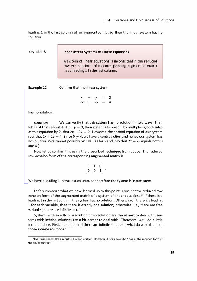
.. Example 11 Confirm that the linear system
x + y = 02x + 2y = 4
has no solu on.
S We can verify that this system has no solu on in two ways. First,let’s just think about it. If x+ y = 0, then it stands to reason, by mul plying both sidesof this equa on by 2, that 2x+ 2y = 0. However, the second equa on of our systemsays that 2x+ 2y = 4. Since 0 = 4, we have a contradic on and hence our system hasno solu on. (We cannot possibly pick values for x and y so that 2x+ 2y equals both 0and 4.)
Now let us confirm this using the prescribed technique from above. The reducedrow echelon form of the corresponding augmented matrix is[
1 1 00 0 1
].
We have a leading 1 in the last column, so therefore the system is inconsistent. ..
Let’s summarize what we have learned up to this point. Consider the reduced rowechelon form of the augmented matrix of a system of linear equa ons.3 If there is aleading 1 in the last column, the systemhas no solu on. Otherwise, if there is a leading1 for each variable, then there is exactly one solu on; otherwise (i.e., there are freevariables) there are infinite solu ons.
Systems with exactly one solu on or no solu on are the easiest to deal with; sys-tems with infinite solu ons are a bit harder to deal with. Therefore, we’ll do a li lemore prac ce. First, a defini on: if there are infinite solu ons, what do we call one ofthose infinite solu ons?
3That sure seems like a mouthful in and of itself. However, it boils down to “look at the reduced form ofthe usual matrix.”
29
Chapter 1 Systems of Linear Equa ons
..Defini on 7
.
.Par cular Solu on
Consider a linear systemof equa onswith infinite solu ons.A par cular solu on is one solu on out of the infinite set ofpossible solu ons.
The easiest way to find a par cular solu on is to pick values for the free variableswhich then determines the values of the dependent variables. Again, more prac ce iscalled for.
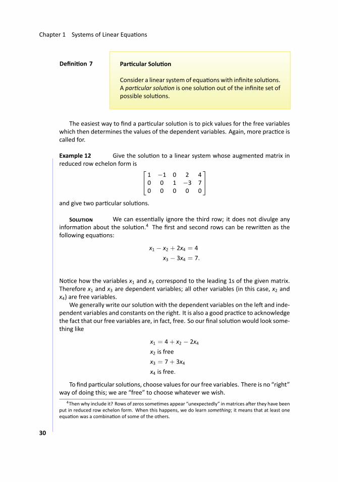
.. Example 12 ..Give the solu on to a linear system whose augmented matrix inreduced row echelon form is 1 −1 0 2 4
0 0 1 −3 70 0 0 0 0
and give two par cular solu ons.
S We can essen ally ignore the third row; it does not divulge anyinforma on about the solu on.4 The first and second rows can be rewri en as thefollowing equa ons:
x1 − x2 + 2x4 = 4
x3 − 3x4 = 7.
No ce how the variables x1 and x3 correspond to the leading 1s of the given matrix.Therefore x1 and x3 are dependent variables; all other variables (in this case, x2 andx4) are free variables.
We generally write our solu on with the dependent variables on the le and inde-pendent variables and constants on the right. It is also a good prac ce to acknowledgethe fact that our free variables are, in fact, free. So our final solu on would look some-thing like
x1 = 4+ x2 − 2x4x2 is free
x3 = 7+ 3x4x4 is free.
To find par cular solu ons, choose values for our free variables. There is no “right”way of doing this; we are “free” to choose whatever we wish.
4Then why include it? Rows of zeros some mes appear “unexpectedly” in matrices a er they have beenput in reduced row echelon form. When this happens, we do learn something; it means that at least oneequa on was a combina on of some of the others.
30
1.4 Existence and Uniqueness of Solu ons
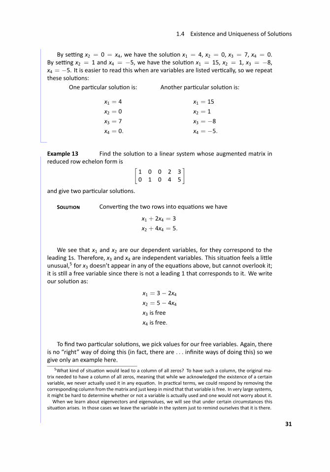
By se ng x2 = 0 = x4, we have the solu on x1 = 4, x2 = 0, x3 = 7, x4 = 0.By se ng x2 = 1 and x4 = −5, we have the solu on x1 = 15, x2 = 1, x3 = −8,x4 = −5. It is easier to read this when are variables are listed ver cally, so we repeatthese solu ons:
One par cular solu on is:
x1 = 4
x2 = 0
x3 = 7
x4 = 0.
Another par cular solu on is:
x1 = 15
x2 = 1
x3 = −8
x4 = −5....
.. Example 13 ..Find the solu on to a linear system whose augmented matrix inreduced row echelon form is [
1 0 0 2 30 1 0 4 5
]and give two par cular solu ons.
S Conver ng the two rows into equa ons we have
x1 + 2x4 = 3
x2 + 4x4 = 5.
We see that x1 and x2 are our dependent variables, for they correspond to theleading 1s. Therefore, x3 and x4 are independent variables. This situa on feels a li leunusual,5 for x3 doesn’t appear in any of the equa ons above, but cannot overlook it;it is s ll a free variable since there is not a leading 1 that corresponds to it. We writeour solu on as:
x1 = 3− 2x4x2 = 5− 4x4x3 is free
x4 is free.
To find two par cular solu ons, we pick values for our free variables. Again, thereis no “right” way of doing this (in fact, there are . . . infinite ways of doing this) so wegive only an example here.
5What kind of situa on would lead to a column of all zeros? To have such a column, the original ma-trix needed to have a column of all zeros, meaning that while we acknowledged the existence of a certainvariable, we never actually used it in any equa on. In prac cal terms, we could respond by removing thecorresponding column from thematrix and just keep in mind that that variable is free. In very large systems,it might be hard to determine whether or not a variable is actually used and one would not worry about it.
When we learn about eigenvectors and eigenvalues, we will see that under certain circumstances thissitua on arises. In those cases we leave the variable in the system just to remind ourselves that it is there.
31
Chapter 1 Systems of Linear Equa ons
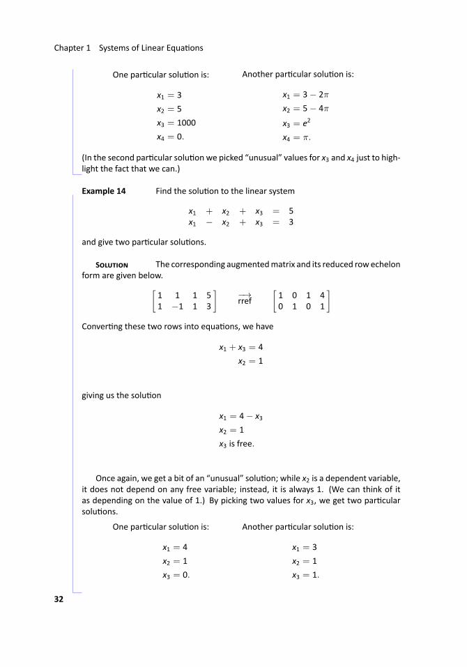
One par cular solu on is:
x1 = 3
x2 = 5
x3 = 1000
x4 = 0.
Another par cular solu on is:
x1 = 3− 2π
x2 = 5− 4π
x3 = e2
x4 = π.
(In the second par cular solu on we picked “unusual” values for x3 and x4 just to high-light the fact that we can.) ...
.. Example 14 Find the solu on to the linear system
x1 + x2 + x3 = 5x1 − x2 + x3 = 3
and give two par cular solu ons.
S The corresponding augmentedmatrix and its reduced rowechelonform are given below.[
1 1 1 51 −1 1 3
]−→rref
[1 0 1 40 1 0 1
]Conver ng these two rows into equa ons, we have
x1 + x3 = 4
x2 = 1
giving us the solu on
x1 = 4− x3x2 = 1
x3 is free.
Once again, we get a bit of an “unusual” solu on; while x2 is a dependent variable,it does not depend on any free variable; instead, it is always 1. (We can think of itas depending on the value of 1.) By picking two values for x3, we get two par cularsolu ons.
One par cular solu on is:
x1 = 4
x2 = 1
x3 = 0.
Another par cular solu on is:
x1 = 3
x2 = 1
x3 = 1...
32
1.4 Existence and Uniqueness of Solu ons
The constants and coefficients of a matrix work together to determine whether agiven system of linear equa ons has one, infinite, or no solu on. The concept will befleshed out more in later chapters, but in short, the coefficients determine whether amatrix will have exactly one solu on or not. In the “or not” case, the constants deter-mine whether or not infinite solu ons or no solu on exists. (So if a given linear systemhas exactly one solu on, it will always have exactly one solu on even if the constantsare changed.) Let’s look at an example to get an idea of how the values of constantsand coefficients work together to determine the solu on type.
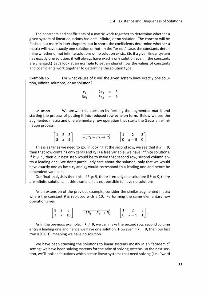
.. Example 15 For what values of k will the given system have exactly one solu-on, infinite solu ons, or no solu on?
x1 + 2x2 = 33x1 + kx2 = 9
S We answer this ques on by forming the augmented matrix andstar ng the process of pu ng it into reduced row echelon form. Below we see theaugmented matrix and one elementary row opera on that starts the Gaussian elimi-na on process.[
1 2 33 k 9
]−−−−−−−−−−−→−3R1 + R2 → R2
[1 2 30 k− 9 0
]This is as far as we need to go. In looking at the second row, we see that if k = 9,
then that row contains only zeros and x2 is a free variable; we have infinite solu ons.If k = 9, then our next step would be to make that second row, second column en-try a leading one. We don’t par cularly care about the solu on, only that we wouldhave exactly one as both x1 and x2 would correspond to a leading one and hence bedependent variables.
Our final analysis is then this. If k = 9, there is exactly one solu on; if k = 9, thereare infinite solu ons. In this example, it is not possible to have no solu ons. ..
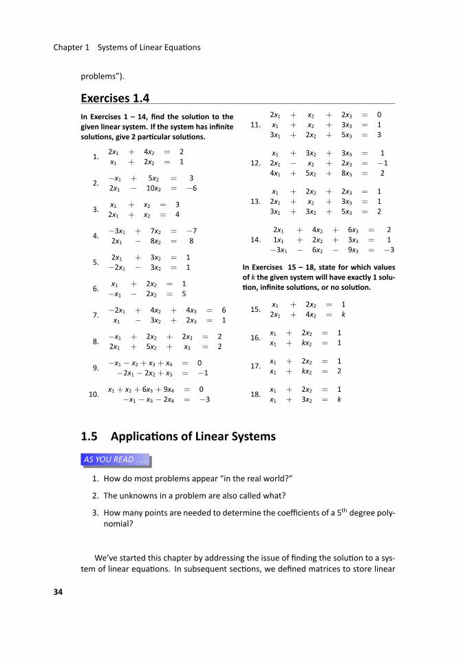
As an extension of the previous example, consider the similar augmented matrixwhere the constant 9 is replaced with a 10. Performing the same elementary rowopera on gives[
1 2 33 k 10
]−−−−−−−−−−−→−3R1 + R2 → R2
[1 2 30 k− 9 1
].
As in the previous example, if k = 9, we can make the second row, second columnentry a leading one and hence we have one solu on. However, if k = 9, then our lastrow is [0 0 1], meaning we have no solu on.
We have been studying the solu ons to linear systems mostly in an “academic”se ng; we have been solving systems for the sake of solving systems. In the next sec-on, we’ll look at situa ons which create linear systems that need solving (i.e., “word
33
Chapter 1 Systems of Linear Equa ons
problems”).
Exercises 1.4In Exercises 1 – 14, find the solu on to thegiven linear system. If the system has infinitesolu ons, give 2 par cular solu ons.
1.2x1 + 4x2 = 2x1 + 2x2 = 1
2.−x1 + 5x2 = 32x1 − 10x2 = −6
3.x1 + x2 = 32x1 + x2 = 4
4.−3x1 + 7x2 = −72x1 − 8x2 = 8
5.2x1 + 3x2 = 1−2x1 − 3x2 = 1
6.x1 + 2x2 = 1−x1 − 2x2 = 5
7.−2x1 + 4x2 + 4x3 = 6x1 − 3x2 + 2x3 = 1
8.−x1 + 2x2 + 2x3 = 22x1 + 5x2 + x3 = 2
9.−x1 − x2 + x3 + x4 = 0
−2x1 − 2x2 + x3 = −1
10.x1 + x2 + 6x3 + 9x4 = 0
−x1 − x3 − 2x4 = −3
11.2x1 + x2 + 2x3 = 0x1 + x2 + 3x3 = 13x1 + 2x2 + 5x3 = 3
12.x1 + 3x2 + 3x3 = 12x1 − x2 + 2x3 = −14x1 + 5x2 + 8x3 = 2
13.x1 + 2x2 + 2x3 = 12x1 + x2 + 3x3 = 13x1 + 3x2 + 5x3 = 2
14.2x1 + 4x2 + 6x3 = 21x1 + 2x2 + 3x3 = 1−3x1 − 6x2 − 9x3 = −3
In Exercises 15 – 18, state for which valuesof k the given system will have exactly 1 solu-on, infinite solu ons, or no solu on.
15.x1 + 2x2 = 12x1 + 4x2 = k
16.x1 + 2x2 = 1x1 + kx2 = 1
17.x1 + 2x2 = 1x1 + kx2 = 2
18.x1 + 2x2 = 1x1 + 3x2 = k
1.5 Applica ons of Linear Systems
...AS YOU READ . . .
1. How do most problems appear “in the real world?”
2. The unknowns in a problem are also called what?
3. Howmany points are needed to determine the coefficients of a 5th degree poly-nomial?
We’ve started this chapter by addressing the issue of finding the solu on to a sys-tem of linear equa ons. In subsequent sec ons, we defined matrices to store linear
34
1.5 Applica ons of Linear Systems
equa on informa on; we described how we can manipulate matrices without chang-ing the solu ons; we described how to efficiently manipulate matrices so that a work-ing solu on can be easily found.
We shouldn’t lose sight of the fact that ourwork in the previous sec onswas aimedat finding solu ons to systems of linear equa ons. In this sec on, we’ll learn how toapply what we’ve learned to actually solve some problems.
Many, many, many problems that are addressed by engineers, businesspeople,scien sts and mathema cians can be solved by properly se ng up systems of linearequa ons. In this sec on we highlight only a few of the wide variety of problems thatmatrix algebra can help us solve.
We start with a simple example.
.. Example 16 ..A jar contains 100 blue, green, red and yellow marbles. There aretwice as many yellow marbles as blue; there are 10 more blue marbles than red; thesum of the red and yellowmarbles is the same as the sum of the blue and green. Howmany marbles of each color are there?
S Let’s call the number of blue balls b, and the number of the otherballs g, r and y, each represen ng the obvious. Since we know that we have 100 mar-bles, we have the equa on
b+ g+ r+ y = 100.
The next sentence in our problem statement allows us to create threemore equa ons.We are told that there are twice as many yellow marbles as blue. One of the fol-
lowing two equa ons is correct, based on this statement; which one is it?
2y = b or 2b = y
The first equa on says that if we take the number of yellow marbles, then doubleit, we’ll have the number of blue marbles. That is not what we were told. The secondequa on states that if we take the number of blue marbles, then double it, we’ll havethe number of yellow marbles. This is what we were told.
The next statement of “there are 10 more blue marbles as red” can be wri en aseither
b = r+ 10 or r = b+ 10.
Which is it?The first equa on says that if we take the number of red marbles, then add 10,
we’ll have the number of blue marbles. This is what we were told. The next equa onis wrong; it implies there are more red marbles than blue.
The final statement tells us that the sum of the red and yellowmarbles is the sameas the sum of the blue and green marbles, giving us the equa on
r+ y = b+ g.
35
Chapter 1 Systems of Linear Equa ons
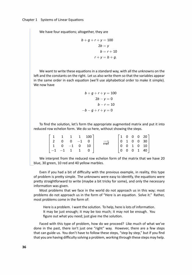
We have four equa ons; altogether, they are
b+ g+ r+ y = 100
2b = y
b = r+ 10
r+ y = b+ g.
Wewant to write these equa ons in a standard way, with all the unknowns on thele and the constants on the right. Let us also write them so that the variables appearin the same order in each equa on (we’ll use alphabe cal order to make it simple).We now have
b+ g+ r+ y = 100
2b− y = 0
b− r = 10
−b− g+ r+ y = 0
To find the solu on, let’s form the appropriate augmented matrix and put it intoreduced row echelon form. We do so here, without showing the steps.
1 1 1 1 1002 0 0 −1 01 0 −1 0 10−1 −1 1 1 0
−→rref
1 0 0 0 200 1 0 0 300 0 1 0 100 0 0 1 40
We interpret from the reduced row echelon form of the matrix that we have 20
blue, 30 green, 10 red and 40 yellow marbles. ...
Even if you had a bit of difficulty with the previous example, in reality, this typeof problem is pre y simple. The unknowns were easy to iden fy, the equa ons werepre y straigh orward to write (maybe a bit tricky for some), and only the necessaryinforma on was given.
Most problems that we face in the world do not approach us in this way; mostproblems do not approach us in the form of “Here is an equa on. Solve it.” Rather,most problems come in the form of:
Here is a problem. I want the solu on. To help, here is lots of informa on.It may be just enough; it may be too much; it may not be enough. Youfigure out what you need; just give me the solu on.
Faced with this type of problem, how do we proceed? Like much of what we’vedone in the past, there isn’t just one “right” way. However, there are a few stepsthat can guide us. You don’t have to follow these steps, “step by step,” but if you findthat you are having difficulty solving a problem, working through these stepsmay help.
36
1.5 Applica ons of Linear Systems
(Note: while the principles outlined herewill help one solve any type of problem, thesesteps are wri en specifically for solving problems that involve only linear equa ons.)
..Key Idea 4
.
.Mathema cal Problem Solving
1. Understand the problem. What exactly is beingasked?
2. Iden fy the unknowns. What are you trying to find?What units are involved?
3. Give names to your unknowns (these are your vari-ables).
4. Use the informa on given to write as many equa onsas you can that involve these variables.
5. Use the equa ons to form an augmented matrix; useGaussian elimina on to put the matrix into reducedrow echelon form.
6. Interpret the reduced row echelon form of the matrixto iden fy the solu on.
7. Ensure the solu on makes sense in the context of theproblem.
Having iden fied some steps, let us put them into prac ce with some examples.
.. Example 17 ..A concert hall has sea ng arranged in three sec ons. As part of aspecial promo on, guests will recieve two of three prizes. Guests seated in the firstand second sec ons will receive Prize A, guests seated in the second and third sec onswill receive Prize B, and guests seated in the first and third sec ons will receive PrizeC. Concert promoters told the concert hall managers of their plans, and asked howmany seats were in each sec on. (The promoters want to store prizes for each sec onseparately for easier distribu on.) The managers, thinking they were being helpful,told the promoters they would need 105 A prizes, 103 B prizes, and 88 C prizes, andhave since been unavailable for further help. How many seats are in each sec on?
S Before we rush in and start making equa ons, we should be clearabout what is being asked. The final sentence asks: “How many seats are in eachsec on?” This tells us what our unknowns should be: we should name our unknownsfor the number of seats in each sec on. Let x1, x2 and x3 denote the number of seatsin the first, second and third sec ons, respec vely. This covers the first two steps ofour general problem solving technique.
37
Chapter 1 Systems of Linear Equa ons
(It is temp ng, perhaps, to name our variables for the number of prizes given away.However, when we think more about this, we realize that we already know this – thatinforma on is given to us. Rather, we should name our variables for the things wedon’t know.)
Having our unknowns iden fied and variables named, we now proceed to formingequa ons from the informa on given. Knowing that Prize A goes to guests in the firstand second sec ons and that we’ll need 105 of these prizes tells us
x1 + x2 = 105.
Proceeding in a similar fashion, we get two more equa ons,
x2 + x3 = 103 and x1 + x3 = 88.
Thus our linear system isx1 + x2 = 105x2 + x3 = 103x1 + x3 = 88
and the corresponding augmented matrix is 1 1 0 1050 1 1 1031 0 1 88
.
To solve our system, let’s put this matrix into reduced row echelon form. 1 1 0 1050 1 1 1031 0 1 88
−→rref
1 0 0 450 1 0 600 0 1 43
We can now read off our solu on. The first sec on has 45 seats, the second has
60 seats, and the third has 43 seats. ...
.. Example 18 ..A lady takes a 2-milemotorizedboat trip down theHighwater River,knowing the trip will take 30 minutes. She asks the boat pilot “How fast does this riverflow?” He replies “I have no idea, lady. I just drive the boat.”
She thinks for a moment, then asks “How long does the return trip take?” Hereplies “The same; half an hour.” She follows up with the statement, “Since both legstake the same me, you must not drive the boat at the same speed.”
“Naw,” the pilot said. “While I really don’t know exactly how fast I go, I do knowthat since we don’t carry any tourists, I drive the boat twice as fast.”
The lady walks away sa sfied; she knows how fast the river flows.(How fast does it flow?)
S This problem forces us to think about what informa on is givenand how to use it to find what we want to know. In fact, to find the solu on, we’ll findout extra informa on that we weren’t asked for!
38
1.5 Applica ons of Linear Systems
We are asked to find how fast the river is moving (step 1). To find this, we shouldrecognize that, in some sense, there are three speeds at work in the boat trips: thespeed of the river (which we want to find), the speed of the boat, and the speed thatthey actually travel at.
We know that each leg of the trip takes half an hour; if it takes half an hour to cover2 miles, then they must be traveling at 4 mph, each way.
The other two speeds are unknowns, but they are related to the overall speeds.Let’s call the speed of the river r and the speed of the boat b. (And we should becareful. From the conversa on, we know that the boat travels at two different speeds.So we’ll say that b represents the speed of the boat when it travels downstream, so2b represents the speed of the boat when it travels upstream.) Let’s let our speed bemeasured in the units of miles/hour (mph) as we used above (steps 2 and 3).
What is the rate of the people on the boat? When they are travelling downstream,their rate is the sum of the water speed and the boat speed. Since their overall speedis 4 mph, we have the equa on r+ b = 4.
When the boat returns going against the current, its overall speed is the rate ofthe boat minus the rate of the river (since the river is working against the boat). Theoverall trip is s ll taken at 4 mph, so we have the equa on 2b − r = 4. (Recall: theboat is traveling twice as fast as before.)
The corresponding augmented matrix is[1 1 42 −1 4
].
Note that we decided to let the first column hold the coefficients of b.Pu ng this matrix in reduced row echelon form gives us:[
1 1 42 −1 4
]−→rref
[1 0 8/30 1 4/3
].
We finish by interpre ng this solu on: the speed of the boat (going downstream)is 8/3mph, or 2.6mph, and the speed of the river is 4/3mph, or 1.3mph. All we reallywanted to know was the speed of the river, at about 1.3 mph. ...
.. Example 19 ..Find the equa on of the quadra c func on that goes through thepoints (−1, 6), (1, 2) and (2, 3).
S This may not seem like a “linear” problem since we are talkingabout a quadra c func on, but closer examina on will show that it really is.
We normally write quadra c func ons as y = ax2 + bx + c where a, b and c arethe coefficients; in this case, they are our unknowns. We have three points; considerthe point (−1, 6). This tells us directly that if x = −1, then y = 6. Therefore we knowthat 6 = a(−1)2+b(−1)+c. Wri ng this in amore standard form, we have the linearequa on
a− b+ c = 6.
The second point tells us that a(1)2 + b(1) + c = 2, which we can simplify asa + b + c = 2, and the last point tells us a(2)2 + b(2) + c = 3, or 4a + 2b + c = 3.
39
Chapter 1 Systems of Linear Equa ons
Thus our linear system isa− b+ c = 6a+ b+ c = 2
4a+ 2b+ c = 3.
Again, to solve our system, we find the reduced row echelon form of the corre-sponding augmented matrix. We don’t show the steps here, just the final result. 1 −1 1 6
1 1 1 24 2 1 3
−−→rref
1 0 0 10 1 0 −20 0 1 3
This tells us that a = 1, b = −2 and c = 3, giving us the quadra c func on
y = x2 − 2x+ 3. ...
One thing interes ng about the previous example is that it confirms for us some-thing that we may have known for a while (but didn’t know why it was true). Why dowe need two points to find the equa on of the line? Because in the equa on of thea line, we have two unknowns, and hence we’ll need two equa ons to find values forthese unknowns.
A quadra c has three unknowns (the coefficients of the x2 term and the x term, andthe constant). Therefore we’ll need three equa ons, and therefore we’ll need threepoints.
What happens if we try to find the quadra c func on that goes through 3 pointsthat are all on the same line? The fast answer is that you’ll get the equa on of a line;there isn’t a quadra c func on that goes through 3 colinear points. Try it and see!(Pick easy points, like (0, 0), (1, 1) and (2, 2). You’ll find that the coefficient of the x2
term is 0.)Of course, we can do the same type of thing to find polynomials that go through 4,
5, etc., points. In general, if you are given n+1 points, a polynomial that goes throughall n+ 1 points will have degree at most n.
.. Example 20 ..A woman has 32 $1, $5 and $10 bills in her purse, giving her a totalof $100. How many bills of each denomina on does she have?
S Let’s name our unknowns x, y and z for our ones, fives and tens,respec vely (it is temp ng to call them o, f and t, but o looks too much like 0). Weknow that there are a total of 32 bills, so we have the equa on
x+ y+ z = 32.
We also know that we have $100, so we have the equa on
x+ 5y+ 10z = 100.
We have three unknowns but only two equa ons, so we know that we cannot expecta unique solu on. Let’s try to solve this system anyway and see what we get.
Pu ng the system into a matrix and then finding the reduced row echelon form,we have [
1 1 1 321 5 10 100
]−→rref
[1 0 − 5
4 150 1 9
4 17
].
40
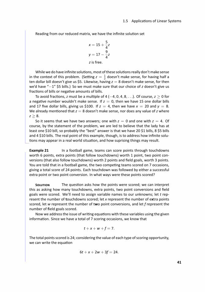
1.5 Applica ons of Linear Systems
Reading from our reduced matrix, we have the infinite solu on set
x = 15+54z
y = 17− 94z
z is free.
Whilewedohave infinite solu ons,most of these solu ons really don’tmake sensein the context of this problem. (Se ng z = 1
2 doesn’t make sense, for having half aten dollar bill doesn’t give us $5. Likewise, having z = 8 doesn’t make sense, for thenwe’d have “−1” $5 bills.) So we must make sure that our choice of z doesn’t give usfrac ons of bills or nega ve amounts of bills.
To avoid frac ons, z must be a mul ple of 4 (−4, 0, 4, 8, . . .). Of course, z ≥ 0 fora nega ve number wouldn’t make sense. If z = 0, then we have 15 one dollar billsand 17 five dollar bills, giving us $100. If z = 4, then we have x = 20 and y = 8.We already men oned that z = 8 doesn’t make sense, nor does any value of z wherez ≥ 8.
So it seems that we have two answers; one with z = 0 and one with z = 4. Ofcourse, by the statement of the problem, we are led to believe that the lady has atleast one $10 bill, so probably the “best” answer is that we have 20 $1 bills, 8 $5 billsand 4 $10 bills. The real point of this example, though, is to address how infinite solu-ons may appear in a real world situa on, and how suprising things may result. ...
.. Example 21 ..In a football game, teams can score points through touchdownsworth 6 points, extra points (that follow touchdowns) worth 1 point, two point con-versions (that also follow touchdowns) worth 2 points and field goals, worth 3 points.You are told that in a football game, the two compe ng teams scored on 7 occasions,giving a total score of 24 points. Each touchdown was followed by either a successfulextra point or two point conversion. In what ways were these points scored?
S The ques on asks how the points were scored; we can interpretthis as asking how many touchdowns, extra points, two point conversions and fieldgoals were scored. We’ll need to assign variable names to our unknowns; let t rep-resent the number of touchdowns scored; let x represent the number of extra pointsscored, let w represent the number of two point conversions, and let f represent thenumber of field goals scored.
Nowwe address the issue of wri ng equa ons with these variables using the giveninforma on. Since we have a total of 7 scoring occasions, we know that
t+ x+ w+ f = 7.
The total points scored is 24; considering the value of each type of scoring opportunity,we can write the equa on
6t+ x+ 2w+ 3f = 24.
41
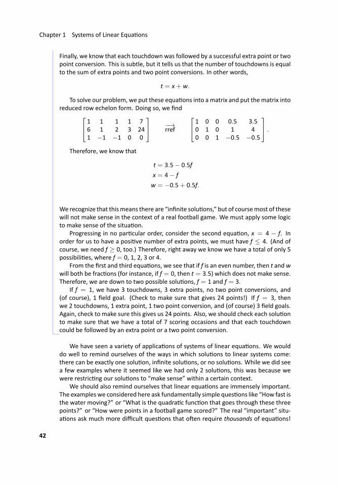
Chapter 1 Systems of Linear Equa ons
Finally, we know that each touchdown was followed by a successful extra point or twopoint conversion. This is subtle, but it tells us that the number of touchdowns is equalto the sum of extra points and two point conversions. In other words,
t = x+ w.
To solve our problem, we put these equa ons into a matrix and put thematrix intoreduced row echelon form. Doing so, we find 1 1 1 1 7
6 1 2 3 241 −1 −1 0 0
−→rref
1 0 0 0.5 3.50 1 0 1 40 0 1 −0.5 −0.5
.
Therefore, we know that
t = 3.5− 0.5f
x = 4− f
w = −0.5+ 0.5f.
We recognize that thismeans there are “infinite solu ons,” but of coursemost of thesewill not make sense in the context of a real football game. We must apply some logicto make sense of the situa on.
Progressing in no par cular order, consider the second equa on, x = 4 − f. Inorder for us to have a posi ve number of extra points, we must have f ≤ 4. (And ofcourse, we need f ≥ 0, too.) Therefore, right away we know we have a total of only 5possibili es, where f = 0, 1, 2, 3 or 4.
From the first and third equa ons, we see that if f is an even number, then t andwwill both be frac ons (for instance, if f = 0, then t = 3.5) which does not make sense.Therefore, we are down to two possible solu ons, f = 1 and f = 3.
If f = 1, we have 3 touchdowns, 3 extra points, no two point conversions, and(of course), 1 field goal. (Check to make sure that gives 24 points!) If f = 3, thenwe 2 touchdowns, 1 extra point, 1 two point conversion, and (of course) 3 field goals.Again, check to make sure this gives us 24 points. Also, we should check each solu onto make sure that we have a total of 7 scoring occasions and that each touchdowncould be followed by an extra point or a two point conversion. ...
We have seen a variety of applica ons of systems of linear equa ons. We woulddo well to remind ourselves of the ways in which solu ons to linear systems come:there can be exactly one solu on, infinite solu ons, or no solu ons. While we did seea few examples where it seemed like we had only 2 solu ons, this was because wewere restric ng our solu ons to “make sense” within a certain context.
We should also remind ourselves that linear equa ons are immensely important.The examples we considered here ask fundamentally simple ques ons like “How fast isthe water moving?” or “What is the quadra c func on that goes through these threepoints?” or “How were points in a football game scored?” The real “important” situ-a ons ask much more difficult ques ons that o en require thousands of equa ons!
42
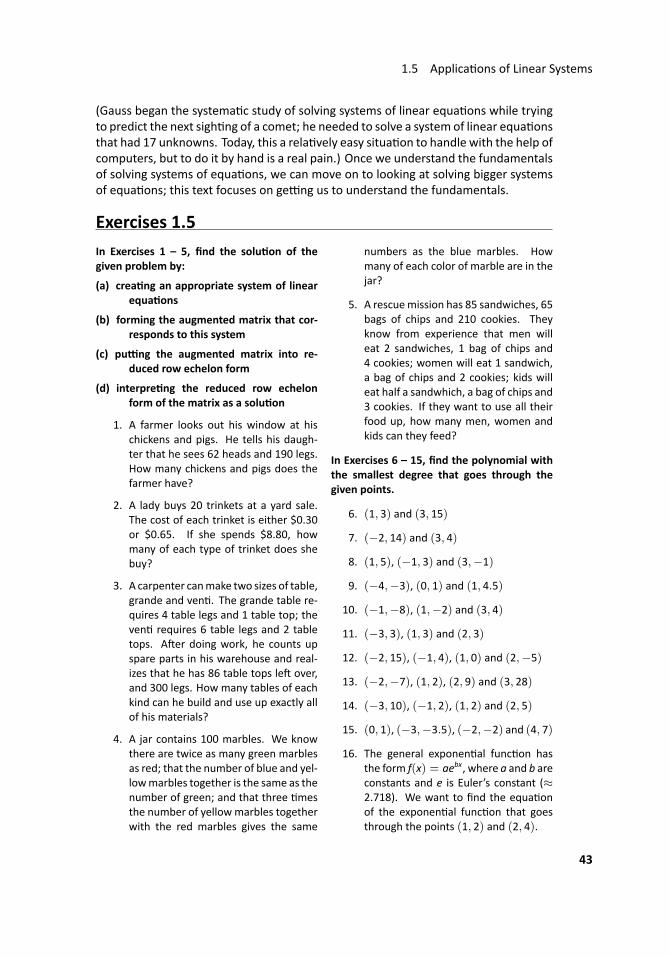
1.5 Applica ons of Linear Systems
(Gauss began the systema c study of solving systems of linear equa ons while tryingto predict the next sigh ng of a comet; he needed to solve a system of linear equa onsthat had 17 unknowns. Today, this a rela vely easy situa on to handle with the help ofcomputers, but to do it by hand is a real pain.) Once we understand the fundamentalsof solving systems of equa ons, we can move on to looking at solving bigger systemsof equa ons; this text focuses on ge ng us to understand the fundamentals.
Exercises 1.5In Exercises 1 – 5, find the solu on of thegiven problem by:
(a) crea ng an appropriate system of linearequa ons
(b) forming the augmented matrix that cor-responds to this system
(c) pu ng the augmented matrix into re-duced row echelon form
(d) interpre ng the reduced row echelonform of the matrix as a solu on
1. A farmer looks out his window at hischickens and pigs. He tells his daugh-ter that he sees 62 heads and 190 legs.How many chickens and pigs does thefarmer have?
2. A lady buys 20 trinkets at a yard sale.The cost of each trinket is either $0.30or $0.65. If she spends $8.80, howmany of each type of trinket does shebuy?
3. A carpenter canmake two sizes of table,grande and ven . The grande table re-quires 4 table legs and 1 table top; theven requires 6 table legs and 2 tabletops. A er doing work, he counts upspare parts in his warehouse and real-izes that he has 86 table tops le over,and 300 legs. How many tables of eachkind can he build and use up exactly allof his materials?
4. A jar contains 100 marbles. We knowthere are twice as many green marblesas red; that the number of blue and yel-lowmarbles together is the same as thenumber of green; and that three mesthe number of yellowmarbles togetherwith the red marbles gives the same
numbers as the blue marbles. Howmany of each color of marble are in thejar?
5. A rescuemission has 85 sandwiches, 65bags of chips and 210 cookies. Theyknow from experience that men willeat 2 sandwiches, 1 bag of chips and4 cookies; women will eat 1 sandwich,a bag of chips and 2 cookies; kids willeat half a sandwhich, a bag of chips and3 cookies. If they want to use all theirfood up, how many men, women andkids can they feed?
In Exercises 6 – 15, find the polynomial withthe smallest degree that goes through thegiven points.
6. (1, 3) and (3, 15)
7. (−2, 14) and (3, 4)
8. (1, 5), (−1, 3) and (3,−1)
9. (−4,−3), (0, 1) and (1, 4.5)
10. (−1,−8), (1,−2) and (3, 4)
11. (−3, 3), (1, 3) and (2, 3)
12. (−2, 15), (−1, 4), (1, 0) and (2,−5)
13. (−2,−7), (1, 2), (2, 9) and (3, 28)
14. (−3, 10), (−1, 2), (1, 2) and (2, 5)
15. (0, 1), (−3,−3.5), (−2,−2) and (4, 7)
16. The general exponen al func on hasthe form f(x) = aebx, where a and b areconstants and e is Euler’s constant (≈2.718). We want to find the equa onof the exponen al func on that goesthrough the points (1, 2) and (2, 4).
43
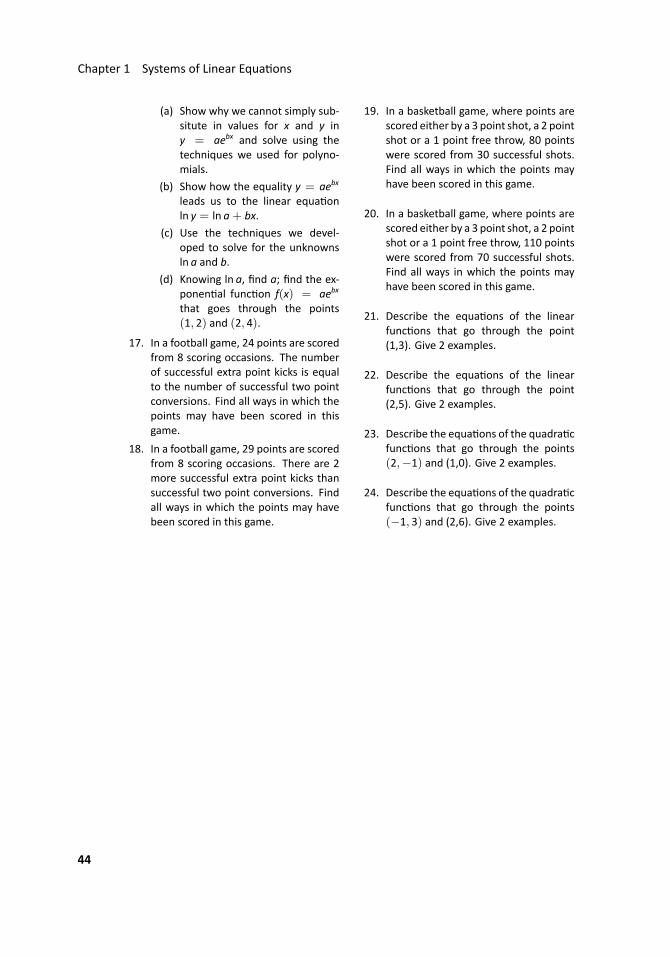
Chapter 1 Systems of Linear Equa ons
(a) Show why we cannot simply sub-situte in values for x and y iny = aebx and solve using thetechniques we used for polyno-mials.
(b) Show how the equality y = aebx
leads us to the linear equa onln y = ln a+ bx.
(c) Use the techniques we devel-oped to solve for the unknownsln a and b.
(d) Knowing ln a, find a; find the ex-ponen al func on f(x) = aebx
that goes through the points(1, 2) and (2, 4).
17. In a football game, 24 points are scoredfrom 8 scoring occasions. The numberof successful extra point kicks is equalto the number of successful two pointconversions. Find all ways in which thepoints may have been scored in thisgame.
18. In a football game, 29 points are scoredfrom 8 scoring occasions. There are 2more successful extra point kicks thansuccessful two point conversions. Findall ways in which the points may havebeen scored in this game.
19. In a basketball game, where points arescored either by a 3 point shot, a 2 pointshot or a 1 point free throw, 80 pointswere scored from 30 successful shots.Find all ways in which the points mayhave been scored in this game.
20. In a basketball game, where points arescored either by a 3 point shot, a 2 pointshot or a 1 point free throw, 110 pointswere scored from 70 successful shots.Find all ways in which the points mayhave been scored in this game.
21. Describe the equa ons of the linearfunc ons that go through the point(1,3). Give 2 examples.
22. Describe the equa ons of the linearfunc ons that go through the point(2,5). Give 2 examples.
23. Describe the equa ons of the quadra cfunc ons that go through the points(2,−1) and (1,0). Give 2 examples.
24. Describe the equa ons of the quadra cfunc ons that go through the points(−1, 3) and (2,6). Give 2 examples.
44
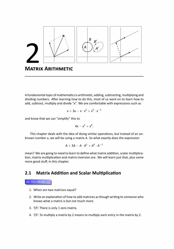
2 ..
A′
.
B′
.
B
.
A
M A
A fundamental topic ofmathema cs is arithme c; adding, subtrac ng,mul plying anddividing numbers. A er learning how to do this, most of us went on to learn how toadd, subtract, mul ply and divide “x”. We are comfortable with expressions such as
x+ 3x− x · x2 + x5 · x−1
and know that we can “simplify” this to
4x− x3 + x4.
This chapter deals with the idea of doing similar opera ons, but instead of an un-known number x, we will be using a matrix A. So what exactly does the expression
A+ 3A− A · A2 + A5 · A−1
mean? We are going to need to learn to define whatmatrix addi on, scalar mul plica-on, matrix mul plica on and matrix inversion are. We will learn just that, plus some
more good stuff, in this chapter.
2.1 Matrix Addi on and Scalar Mul plica on
...AS YOU READ . . .
1. When are two matrices equal?
2. Write an explana on of how to addmatrices as though wri ng to someone whoknows what a matrix is but not much more.
3. T/F: There is only 1 zero matrix.
4. T/F: To mul ply a matrix by 2 means to mul ply each entry in the matrix by 2.
Chapter 2 Matrix Arithme c
In the past, when we dealt with expressions that used “x,” we didn’t just add andmul ply x’s together for the fun of it, but rather because we were usually given somesort of equa on that had x in it and we had to “solve for x.”
This begs the ques on, “What does it mean to be equal?” Two numbers are equal,when, . . ., uh, . . ., nevermind. What does it mean for two matrices to be equal? Wesay that matrices A and B are equal when their corresponding entries are equal. Thisseems like a very simple defini on, but it is rather important, so we give it a box.
..Defini on 8
..
Matrix EqualityTwom×nmatrices A and B are equal if their correspondingentries are equal.
No ce that our more formal defini on specifies that if matrices are equal, theyhave the same dimensions. This should make sense.
Nowwemove on to describing how to add twomatrices together. To start off, takea wild stab: what do you think the following sum is equal to?[
1 23 4
]+
[2 −15 7
]= ?
If you guessed [3 18 11
],
you guessed correctly. That wasn’t so hard, was it?Let’s keep going, hoping that we are star ng to get on a roll. Make another wild
guess: what do you think the following expression is equal to?
3 ·[1 23 4
]= ?
If you guessed [3 69 12
],
you guessed correctly!Even if you guessed wrong both mes, you probably have seen enough in these
two examples to have a fair idea now what matrix addi on and scalar mul plica onare all about.
Before we formally define how to perform the above opera ons, let us first recallthat if A is anm× nmatrix, then we can write A as
A =
a11 a12 · · · a1na21 a22 · · · a2n...
.... . .
...am1 am2 · · · amn
.
46
2.1 Matrix Addi on and Scalar Mul plica on
Secondly, we should define what we mean by the word scalar. A scalar is any numberthat we mul ply a matrix by. (In some sense, we use that number to scale the matrix.)We are now ready to define our first arithme c opera ons.
..Defini on 9
.
.Matrix Addi on
Let A and B bem×nmatrices. The sum of A and B, denotedA+ B, is
a11 + b11 a12 + b12 · · · a1n + b1na21 + b21 a22 + b22 · · · a2n + b2n
......
. . ....
am1 + bm1 am2 + bm2 · · · amn + bmn
.
..Defini on 10
.
.Scalar Mul plica on
Let A be an m × n matrix and let k be a scalar. The scalarmul plica on of k and A, denoted kA, is
ka11 ka12 · · · ka1nka21 ka22 · · · ka2n...
.... . .
...kam1 kam2 · · · kamn
.
We are now ready for an example.
.. Example 22 ..Let
A =
1 2 3−1 2 15 5 5
, B =
2 4 61 2 2−1 0 4
, C =
[1 2 39 8 7
].
Simplify the following matrix expressions.
1. A+ B
2. B+ A
3. A− B
4. A+ C
5. −3A+ 2B
6. A− A
7. 5A+ 5B
8. 5(A+ B)
S
47
Chapter 2 Matrix Arithme c
1. A+ B =
3 6 90 4 34 5 9
.2. B+ A =
3 6 90 4 34 5 9
.3. A− B =
−1 −2 −3−2 0 −16 5 1
.4. A + C is not defined. If we look at our defini on of matrix addi on, we see
that the two matrices need to be the same size. Since A and C have differentdimensions, we don’t even try to create something as an addi on; we simplysay that the sum is not defined.
5. −3A+ 2B =
1 2 35 −2 1
−17 −15 −7
.6. A− A =
0 0 00 0 00 0 0
.7. Strictly speaking, this is
5 10 15−5 10 525 25 25
+ 10 20 30
5 10 10−5 0 20
=
15 30 450 20 1520 25 45
.8. Strictly speaking, this is
5
1 2 3−1 2 15 5 5
+
2 4 61 2 2−1 0 4
= 5 ·
3 6 90 4 34 5 9
=
15 30 450 20 1520 25 45
.
...
Our example raised a few interes ng points. No ce how A + B = B + A. Weprobably aren’t suprised by this, since we know that when dealing with numbers, a+b = b+ a. Also, no ce that 5A+ 5B = 5(A+ B). In our example, we were careful tocompute each of these expressions following the proper order of opera ons; knowingthese are equal allows us to compute similar expressions in the most convenient way.
Another interes ng thing that came from our previous example is that
A− A =
0 0 00 0 00 0 0
.
48
2.1 Matrix Addi on and Scalar Mul plica on
It seems like this should be a special matrix; a er all, every entry is 0 and 0 is a specialnumber.
In fact, this is a special matrix. We define 0, which we read as “the zero matrix,”to be the matrix of all zeros.1 We should be careful; this previous “defini on” is a bit
ambiguous, for we have not stated what size the zero matrix should be. Is[0 00 0
]the zero matrix? How about
[0 0
]?
Let’s not get bogged down in seman cs. If we ever see 0 in an expression, wewill usually know right away what size 0 should be; it will be the size that allows theexpression to make sense. If A is a 3 × 5 matrix, and we write A + 0, we’ll simplyassume that 0 is also a 3 × 5 matrix. If we are ever in doubt, we can add a subscript;for instance, 02×7 is the 2× 7 matrix of all zeros.
Since the zero matrix is an important concept, we give it it’s own defini on box.
..Defini on 11
.
.The Zero Matrix
The m × n matrix of all zeros, denoted 0m×n, is the zeromatrix.
When the dimensions of the zero matrix are clear from thecontext, the subscript is generally omi ed.
The following presents some of the proper es of matrix addi on and scalar mul -plica on that we discovered above, plus a few more.
..Theorem 2
.
.Proper es of Matrix Addi on and Scalar Mul plica on
The following equali es hold for allm× nmatrices A, B andC and scalars k.
1. A+ B = B+ A (Commuta ve Property)
2. (A+ B) + C = A+ (B+ C) (Associa ve Property)
3. k(A+B) = kA+ kB (Scalar Mul plica on Distribu veProperty)
4. kA = Ak
5. A+ 0 = 0+ A = A (Addi ve Iden ty)
6. 0A = 0
Be sure that this last property makes sense; it says that if we mul ply any matrix
1We use the bold face to dis nguish the zero matrix, 0, from the number zero, 0.49
Chapter 2 Matrix Arithme c
by the number 0, the result is the zero matrix, or 0.We began this sec on with the concept of matrix equality. Let’s put our matrix
addi on proper es to use and solve a matrix equa on.
.. Example 23 Let
A =
[2 −13 6
].
Find the matrix X such that2A+ 3X = −4A.
S We can use basic algebra techniques to manipulate this equa onfor X; first, let’s subtract 2A from both sides. This gives us
3X = −6A.
Now divide both sides by 3 to get
X = −2A.
Now we just need to compute−2A; we find that
X =
[−4 2−6 −12
].
..
Our matrix proper es iden fied 0 as the Addi ve Iden ty; i.e., if you add 0 to anymatrix A, you simply get A. This is similar in no on to the fact that for all numbers a,a+ 0 = a. AMul plica ve Iden ty would be a matrix I where I× A = A for all matri-ces A. (What would such a matrix look like? A matrix of all 1s, perhaps?) However, inorder for this to make sense, we’ll need to learn to mul ply matrices together, whichwe’ll do in the next sec on.
Exercises 2.1Matrices A and B are given below. In Exer-cises 1 – 6, simplify the given expression.
A =
[1 −17 4
]B =
[−3 25 9
]
1. A+ B
2. 2A− 3B
3. 3A− A
4. 4B− 2A
5. 3(A− B) + B
6. 2(A− B)− (A− 3B)
Matrices A and B are given below. In Exer-cises 7 – 10, simplify the given expression.
A =
[35
]B =
[−24
]
7. 4B− 2A
8. −2A+ 3A
50
2.2 Matrix Mul plica on
9. −2A− 3A
10. −B+ 3B− 2B
Matrices A and B are given below. In Exer-cises 11 – 14, find X that sa sfies the equa-on.
A =
[3 −12 5
]B =
[1 73 −4
]
11. 2A+ X = B
12. A− X = 3B
13. 3A+ 2X = −1B
14. A− 12X = −B
In Exercises 15 – 21, find values for the scalarsa and b that sa sfy the given equa on.
15. a[12
]+ b
[−15
]=
[19
]16. a
[−31
]+ b
[84
]=
[71
]17. a
[4−2
]+ b
[−63
]=
[10−5
]18. a
[11
]+ b
[−13
]=
[55
]19. a
[13
]+ b
[−3−9
]=
[4
−12
]
20. a
123
+ b
112
=
0−1−1
21. a
101
+ b
512
=
347
2.2 Matrix Mul plica on
...AS YOU READ . . .
1. T/F: Column vectors are used more in this text than row vectors, although someother texts do the opposite.
2. T/F: To mul ply A× B, the number of rows of A and B need to be the same.
3. T/F: The entry in the 2nd row and 3rd column of the product AB comes frommul pling the 2nd row of A with the 3rd column of B.
4. Name two proper es of matrix mul plica on that also hold for “regular mul -plica on” of numbers.
5. Name a property of “regular mul plica on” of numbers that does not hold formatrix mul plica on.
6. T/F: A3 = A · A · A
In the previous sec on we found that the defini on of matrix addi on was veryintui ve, and we ended that sec on discussing the fact that eventually we’d like toknow what it means to mul ply matrices together.
In the spirit of the last sec on, take another wild stab: what do you think[1 23 4
]×[1 −12 2
]51
Chapter 2 Matrix Arithme c
means?You are likely to have guessed [
1 −26 8
]but this is, in fact, not right.2 The actual answer is[
5 311 5
].
If you can look at this one example and suddenly understand exactly how matrix mul-plica on works, then you are probably smarter than the author. While matrix mul -
plica on isn’t hard, it isn’t nearly as intui ve as matrix addi on is.To further muddy the waters (before we clear them), consider[
1 23 4
]×[1 −1 02 2 −1
].
Our experience from the last sec on would lend us to believe that this is not defined,but our confidence is probably a bit shaken by now. In fact, this mul plica on is de-fined, and it is [
5 3 −211 5 −4
].
You may see some similarity in this answer to what we got before, but again, probablynot enough to really figure things out.
So let’s take a step back and progress slowly. The first thing we’d like to do is definea special type of matrix called a vector.
..Defini on 12
.
.Column and Row Vectors
Am× 1 matrix is called a column vector.
A 1× nmatrix is called a row vector.
While it isn’t obvious right now, column vectors are going to become far more use-ful to us than row vectors. Therefore, we o en omit the word “column” when referingto column vectors, and we just call them “vectors.”3
2I guess you could define mul plica on this way. If you’d prefer this type of mul plica on, write yourown book.
3In this text, row vectors are only used in this sec on when we discuss matrix mul plica on, whereaswe’ll make extensive use of column vectors. Other texts make great use of row vectors, but li le use ofcolumn vectors. It is a ma er of preference and tradi on: “most” texts use column vectors more.
52
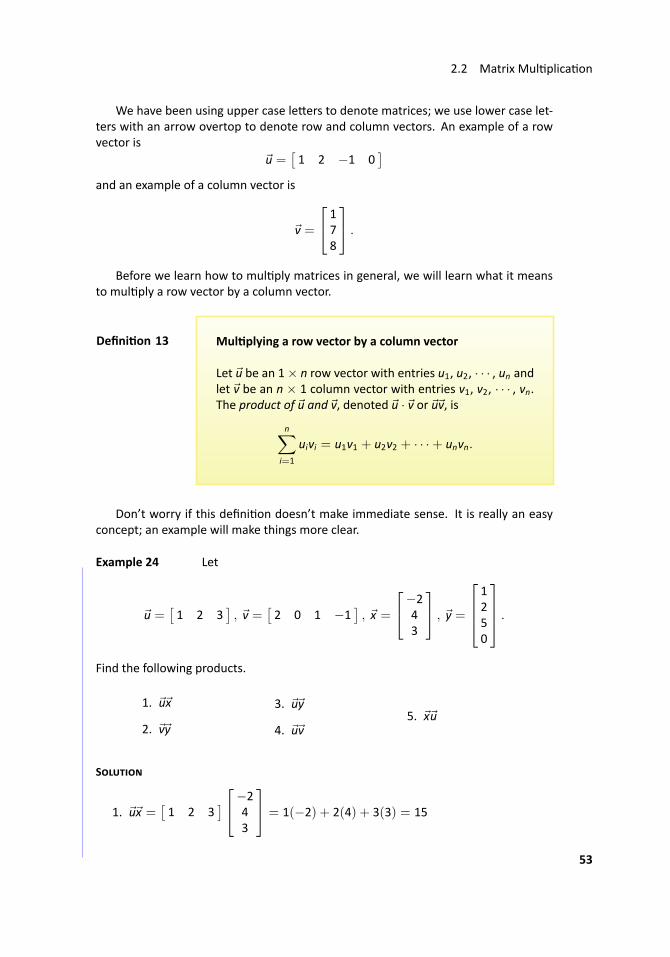
2.2 Matrix Mul plica on
We have been using upper case le ers to denote matrices; we use lower case let-ters with an arrow overtop to denote row and column vectors. An example of a rowvector is
u =[1 2 −1 0
]and an example of a column vector is
v =
178
.
Before we learn how to mul ply matrices in general, we will learn what it meansto mul ply a row vector by a column vector.
..Defini on 13
.
.Mul plying a row vector by a column vector
Let u be an 1× n row vector with entries u1, u2, · · · , un andlet v be an n × 1 column vector with entries v1, v2, · · · , vn.The product of u and v, denoted u · v or uv, is
n∑i=1
uivi = u1v1 + u2v2 + · · ·+ unvn.
Don’t worry if this defini on doesn’t make immediate sense. It is really an easyconcept; an example will make things more clear.
.. Example 24 ..Let
u =[1 2 3
], v =
[2 0 1 −1
], x =
−243
, y =
1250
.
Find the following products.
1. ux
2. vy
3. uy
4. uv5. xu
S
1. ux =[1 2 3
] −243
= 1(−2) + 2(4) + 3(3) = 15
53
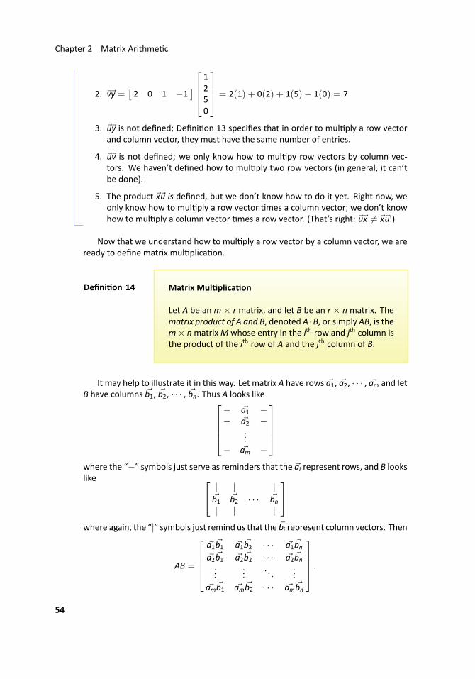
Chapter 2 Matrix Arithme c
2. vy =[2 0 1 −1
] 1250
= 2(1) + 0(2) + 1(5)− 1(0) = 7
3. uy is not defined; Defini on 13 specifies that in order to mul ply a row vectorand column vector, they must have the same number of entries.
4. uv is not defined; we only know how to mul py row vectors by column vec-tors. We haven’t defined how to mul ply two row vectors (in general, it can’tbe done).
5. The product xu is defined, but we don’t know how to do it yet. Right now, weonly know how to mul ply a row vector mes a column vector; we don’t knowhow to mul ply a column vector mes a row vector. (That’s right: ux = xu!)...
Now that we understand how to mul ply a row vector by a column vector, we areready to define matrix mul plica on.
..Defini on 14
.
.Matrix Mul plica on
Let A be an m × r matrix, and let B be an r × n matrix. Thematrix product of A and B, denoted A ·B, or simply AB, is them× nmatrixM whose entry in the ith row and jth column isthe product of the ith row of A and the jth column of B.
It may help to illustrate it in this way. Let matrix A have rows a1, a2, · · · , am and letB have columns b1, b2, · · · , bn. Thus A looks like
− a1 −− a2 −
...− am −
where the “−” symbols just serve as reminders that the ai represent rows, and B lookslike | | |
b1 b2 · · · bn| | |
where again, the “|” symbols just remind us that the bi represent column vectors. Then
AB =
a1b1 a1b2 · · · a1bna2b1 a2b2 · · · a2bn...
.... . .
...amb1 amb2 · · · ambn
.
54
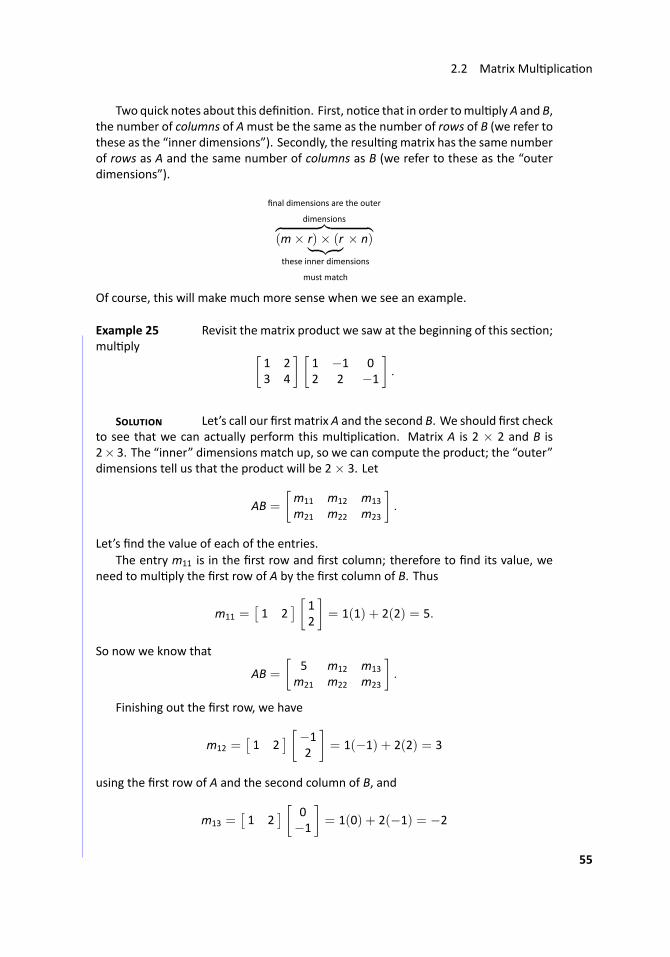
2.2 Matrix Mul plica on
Two quick notes about this defini on. First, no ce that in order tomul ply A and B,the number of columns of Amust be the same as the number of rows of B (we refer tothese as the “inner dimensions”). Secondly, the resul ng matrix has the same numberof rows as A and the same number of columns as B (we refer to these as the “outerdimensions”).
final dimensions are the outer
dimensions︷ ︸︸ ︷(m× r)× (r︸ ︷︷ ︸these inner dimensions
must match
× n)
Of course, this will make much more sense when we see an example.
.. Example 25 ..Revisit the matrix product we saw at the beginning of this sec on;mul ply [
1 23 4
] [1 −1 02 2 −1
].
S Let’s call our first matrix A and the second B. We should first checkto see that we can actually perform this mul plica on. Matrix A is 2 × 2 and B is2× 3. The “inner” dimensions match up, so we can compute the product; the “outer”dimensions tell us that the product will be 2× 3. Let
AB =
[m11 m12 m13
m21 m22 m23
].
Let’s find the value of each of the entries.The entry m11 is in the first row and first column; therefore to find its value, we
need to mul ply the first row of A by the first column of B. Thus
m11 =[1 2
] [ 12
]= 1(1) + 2(2) = 5.
So now we know that
AB =
[5 m12 m13
m21 m22 m23
].
Finishing out the first row, we have
m12 =[1 2
] [−12
]= 1(−1) + 2(2) = 3
using the first row of A and the second column of B, and
m13 =[1 2
] [ 0−1
]= 1(0) + 2(−1) = −2
55
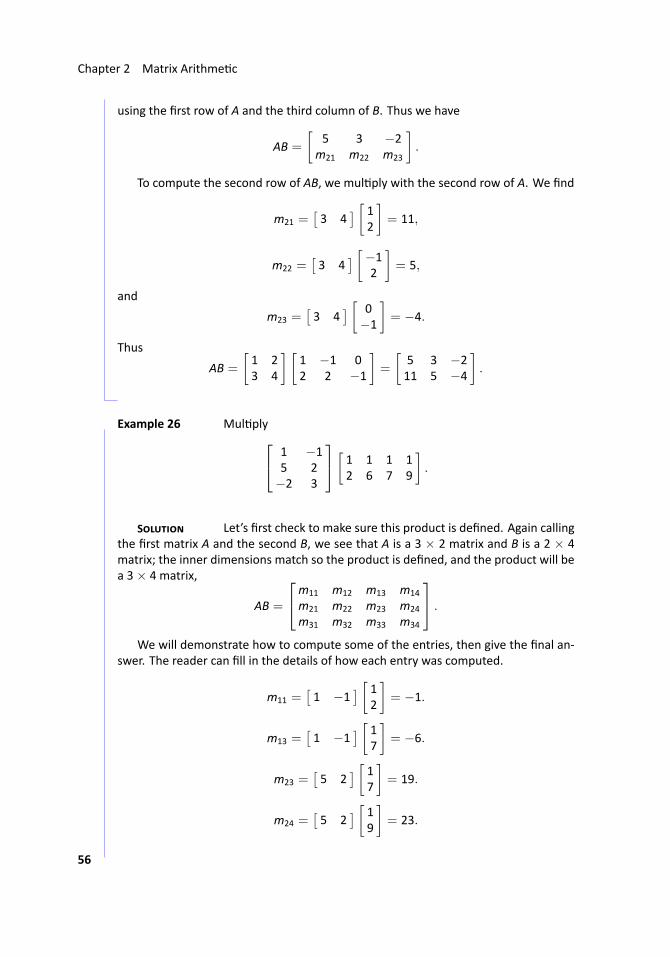
Chapter 2 Matrix Arithme c
using the first row of A and the third column of B. Thus we have
AB =
[5 3 −2
m21 m22 m23
].
To compute the second row of AB, we mul ply with the second row of A. We find
m21 =[3 4
] [ 12
]= 11,
m22 =[3 4
] [−12
]= 5,
and
m23 =[3 4
] [ 0−1
]= −4.
Thus
AB =
[1 23 4
] [1 −1 02 2 −1
]=
[5 3 −211 5 −4
].
...
.. Example 26 ..Mul ply 1 −15 2−2 3
[1 1 1 12 6 7 9
].
S Let’s first check to make sure this product is defined. Again callingthe first matrix A and the second B, we see that A is a 3 × 2 matrix and B is a 2 × 4matrix; the inner dimensions match so the product is defined, and the product will bea 3× 4 matrix,
AB =
m11 m12 m13 m14
m21 m22 m23 m24
m31 m32 m33 m34
.
We will demonstrate how to compute some of the entries, then give the final an-swer. The reader can fill in the details of how each entry was computed.
m11 =[1 −1
] [ 12
]= −1.
m13 =[1 −1
] [ 17
]= −6.
m23 =[5 2
] [ 17
]= 19.
m24 =[5 2
] [ 19
]= 23.
56
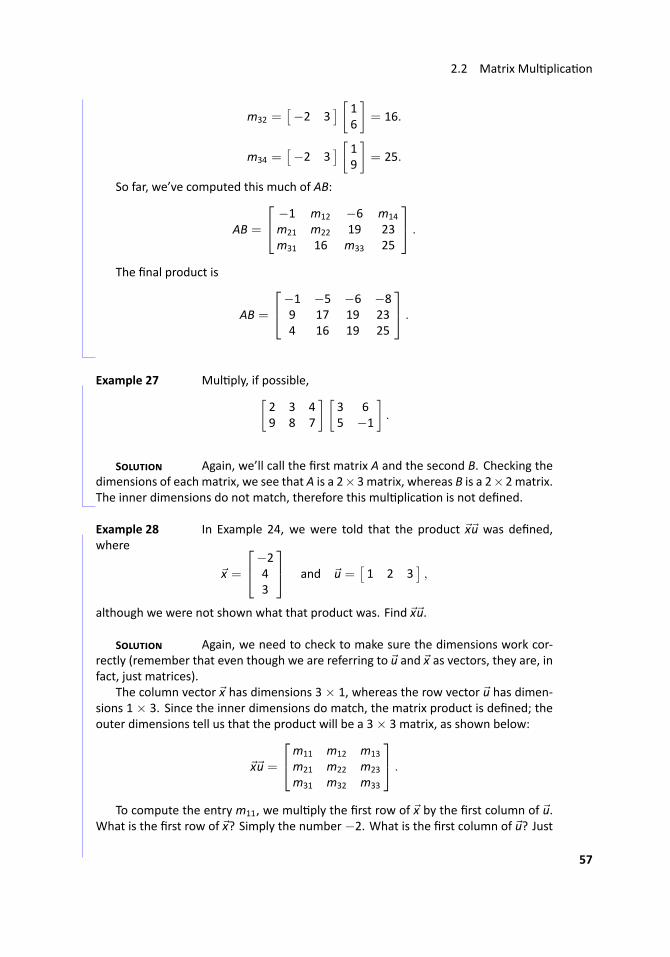
2.2 Matrix Mul plica on
m32 =[−2 3
] [ 16
]= 16.
m34 =[−2 3
] [ 19
]= 25.
So far, we’ve computed this much of AB:
AB =
−1 m12 −6 m14
m21 m22 19 23m31 16 m33 25
.
The final product is
AB =
−1 −5 −6 −89 17 19 234 16 19 25
.
...
.. Example 27 Mul ply, if possible,[2 3 49 8 7
] [3 65 −1
].
S Again, we’ll call the first matrix A and the second B. Checking thedimensions of each matrix, we see that A is a 2×3 matrix, whereas B is a 2×2 matrix.The inner dimensions do not match, therefore this mul plica on is not defined. ..
.. Example 28 ..In Example 24, we were told that the product xu was defined,where
x =
−243
and u =[1 2 3
],
although we were not shown what that product was. Find xu.
S Again, we need to check to make sure the dimensions work cor-rectly (remember that even though we are referring to u and x as vectors, they are, infact, just matrices).
The column vector x has dimensions 3 × 1, whereas the row vector u has dimen-sions 1 × 3. Since the inner dimensions do match, the matrix product is defined; theouter dimensions tell us that the product will be a 3× 3 matrix, as shown below:
xu =
m11 m12 m13
m21 m22 m23
m31 m32 m33
.
To compute the entry m11, we mul ply the first row of x by the first column of u.What is the first row of x? Simply the number−2. What is the first column of u? Just
57
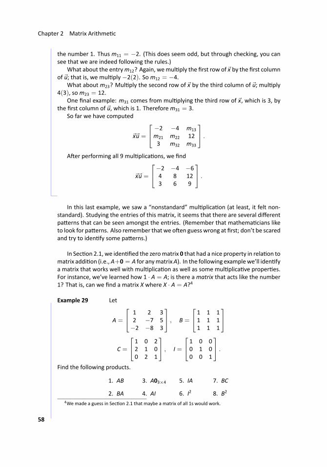
Chapter 2 Matrix Arithme c
the number 1. Thus m11 = −2. (This does seem odd, but through checking, you cansee that we are indeed following the rules.)
What about the entrym12? Again, wemul ply the first row of x by the first columnof u; that is, we mul ply−2(2). Som12 = −4.
What about m23? Mul ply the second row of x by the third column of u; mul ply4(3), som23 = 12.
One final example: m31 comes from mul plying the third row of x, which is 3, bythe first column of u, which is 1. Thereforem31 = 3.
So far we have computed
xu =
−2 −4 m13
m21 m22 123 m32 m33
.
A er performing all 9 mul plica ons, we find
xu =
−2 −4 −64 8 123 6 9
.
...
In this last example, we saw a “nonstandard” mul plica on (at least, it felt non-standard). Studying the entries of this matrix, it seems that there are several differentpa erns that can be seen amongst the entries. (Remember that mathema cians liketo look for pa erns. Also remember that we o en guess wrong at first; don’t be scaredand try to iden fy some pa erns.)
In Sec on 2.1, we iden fied the zeromatrix 0 that had a nice property in rela on tomatrix addi on (i.e., A+0 = A for anymatrixA). In the following examplewe’ll iden fya matrix that works well with mul plica on as well as some mul plica ve proper es.For instance, we’ve learned how 1 · A = A; is there amatrix that acts like the number1? That is, can we find a matrix X where X · A = A?4
.. Example 29 ..Let
A =
1 2 32 −7 5−2 −8 3
, B =
1 1 11 1 11 1 1
C =
1 0 22 1 00 2 1
, I =
1 0 00 1 00 0 1
.
Find the following products.
1. AB
2. BA
3. A03×4
4. AI
5. IA
6. I2
7. BC
8. B2
4We made a guess in Sec on 2.1 that maybe a matrix of all 1s would work.
58
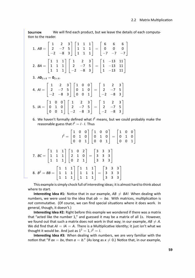
2.2 Matrix Mul plica on
S We will find each product, but we leave the details of each computa-on to the reader.
1. AB =
1 2 32 −7 5−2 −8 3
1 1 11 1 11 1 1
=
6 6 60 0 0−7 −7 −7
2. BA =
1 1 11 1 11 1 1
1 2 32 −7 5−2 −8 3
=
1 −13 111 −13 111 −13 11
3. A03×4 = 03×4.
4. AI =
1 2 32 −7 5−2 −8 3
1 0 00 1 00 0 1
=
1 2 32 −7 5−2 −8 3
5. IA =
1 0 00 1 00 0 1
1 2 32 −7 5−2 −8 3
=
1 2 32 −7 5−2 −8 3
6. We haven’t formally defined what I2 means, but we could probably make the
reasonable guess that I2 = I · I. Thus
I2 =
1 0 00 1 00 0 1
1 0 00 1 00 0 1
=
1 0 00 1 00 0 1
7. BC =
1 1 11 1 11 1 1
1 0 22 1 00 2 1
=
3 3 33 3 33 3 3
8. B2 = BB =
1 1 11 1 11 1 1
1 1 11 1 11 1 1
=
3 3 33 3 33 3 3
...
This example is simply chock full of interes ng ideas; it is almost hard to think aboutwhere to start.
Interes ng Idea #1: No ce that in our example, AB = BA! When dealing withnumbers, we were used to the idea that ab = ba. With matrices, mul plica on isnot commuta ve. (Of course, we can find special situa ons where it does work. Ingeneral, though, it doesn’t.)
Interes ng Idea #2: Right before this example we wondered if there was a matrixthat “acted like the number 1,” and guessed it may be a matrix of all 1s. However,we found out that such a matrix does not work in that way; in our example, AB = A.We did find that AI = IA = A. There is a Mul plica ve Iden ty; it just isn’t what wethought it would be. And just as 12 = 1, I2 = I.
Interes ng Idea #3: When dealing with numbers, we are very familiar with theno on that “If ax = bx, then a = b.” (As long as x = 0.) No ce that, in our example,
59
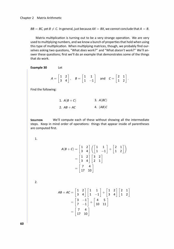
Chapter 2 Matrix Arithme c
BB = BC, yet B = C. In general, just becauseAX = BX, we cannot conclude thatA = B.
Matrix mul plica on is turning out to be a very strange opera on. We are veryused tomul plying numbers, andwe know a bunch of proper es that hold when usingthis type of mul plica on. When mul plying matrices, though, we probably find our-selves asking two ques ons, “What does work?” and “What doesn’t work?” We’ll an-swer these ques ons; first we’ll do an example that demonstrates some of the thingsthat do work.
.. Example 30 ..Let
A =
[1 23 4
], B =
[1 11 −1
]and C =
[2 11 2
].
Find the following:
1. A(B+ C)
2. AB+ AC
3. A(BC)
4. (AB)C
S We’ll compute each of these without showing all the intermediatesteps. Keep in mind order of opera ons: things that appear inside of parenthesesare computed first.
1.
A(B+ C) =[1 23 4
]([1 11 −1
]+
[2 11 2
])=
[1 23 4
] [3 22 1
]=
[7 417 10
]
2.
AB+ AC =
[1 23 4
] [1 11 −1
]+
[1 23 4
] [2 11 2
]=
[3 −17 −1
]+
[4 510 11
]=
[7 417 10
]
60
2.2 Matrix Mul plica on
3.
A(BC) =[1 23 4
]([1 11 −1
] [2 11 2
])=
[1 23 4
] [3 31 −1
]=
[5 113 5
]
4.
(AB) C =
([1 23 4
] [1 11 −1
])[2 11 2
]=
[3 −17 −1
] [2 11 2
]=
[5 113 5
]...
In looking at our example, we should no ce two things. First, it looks like the “dis-tribu ve property” holds; that is, A(B+ C) = AB+ AC. This is nice as many algebraictechniques we have learned about in the past (when doing “ordinary algebra”) will s llwork. Secondly, it looks like the “associa ve property” holds; that is, A(BC) = (AB)C.This is nice, for it tells us that when we are mul plying several matrices together, wedon’t have to be par cularly careful in what order wemul ply certain pairs of matricestogether.5
In leading to an important theorem, let’s define a matrix we saw in an earlier ex-ample.6
..Defini on 15
.
.Iden ty Matrix
The n × n matrix with 1’s on the diagonal and zeros else-where is the n × n iden ty matrix, denoted In. When thecontext makes the dimension of the iden ty clear, the sub-script is generally omi ed.
Note that while the zero matrix can come in all different shapes and sizes, the
5Be careful: in compu ng ABC together, we can first mul ply AB or BC, but we cannot change the orderin which these matrices appear. We cannot mul ply BA or AC, for instance.
6The following defini on uses a termwewon’t define un l Defini on 20 on page 123: diagonal. In short,a “diagonal matrix” is one in which the only nonzero entries are the “diagonal entries.” The examples givenhere and in the exercises should suffice un l we meet the full defini on later.
61
Chapter 2 Matrix Arithme c
iden ty matrix is always a square matrix. We show a few iden ty matrices below.
I2 =[1 00 1
], I3 =
1 0 00 1 00 0 1
, I4 =
1 0 0 00 1 0 00 0 1 00 0 0 1
In our examples above, we have seen examples of things that do and do not work.
We should be careful about what examples prove, though. If someone were to claimthat AB = BA is always true, one would only need to show them one example wherethey were false, and we would know the person was wrong. However, if someoneclaims that A(B + C) = AB + AC is always true, we can’t prove this with just oneexample. We need something more powerful; we need a true proof.
In this text, we forgo most proofs. The reader should know, though, that whenwe state something in a theorem, there is a proof that backs up what we state. Ourjus fica on comes from something stronger than just examples.
Now we give the good news of what does work when dealing with matrix mul pli-ca on.
..Theorem 3
.
.Proper es of Matrix Mul plica on
Let A, B and C be matrices with dimensions so that the fol-lowing opera ons make sense, and let k be a scalar. Thefollowing equali es hold:
1. A(BC) = (AB)C (Associa ve Property)
2. A(B+ C) = AB+ AB and
(B+ C)A = BA+ CA (Distribu ve Property)
3. k(AB) = (kA)B = A(kB)
4. AI = IA = A
The above box contains some very good news, and probably some very surprisingnews. Matrix mul plica on probably seems to us like a very odd opera on, so weprobably wouldn’t have been surprised if we were told that A(BC) = (AB)C. It is avery nice thing that the Associa ve Property does hold.
As we near the end of this sec on, we raise one more issue of nota on. We defineA0 = I. If n is a posi ve integer, we define
An = A · A · · · · · A︸ ︷︷ ︸n mes
.
With numbers, we are used to a−n = 1an . Do nega ve exponents work with matri-
ces, too? The answer is yes, sort of. We’ll have to be careful, and we’ll cover the topic
62
2.2 Matrix Mul plica on
in detail once we define the inverse of a matrix. For now, though, we recognize thefact that A−1 = 1
A , for1A makes no sense; we don’t know how to “divide” by a matrix.
We end this sec on with a reminder of some of the things that do not work withmatrix mul plica on. The good news is that there are really only two things on thislist.
1. Matrix mul plica on is not commuta ve; that is, AB = BA.
2. In general, just because AX = BX, we cannot conclude that A = B.
The bad news is that these ideas pop up in many places where we don’t expect them.For instance, we are used to
(a+ b)2 = a2 + 2ab+ b2.
What about (A+ B)2? All we’ll say here is that
(A+ B)2 = A2 + 2AB+ B2;
we leave it to the reader to figure out why.The next sec on is devoted to visualizing column vectors and “seeing” how some
of these arithme c proper es work together.
Exercises 2.2In Exercises 1 – 12, row and column vectors uand v are defined. Find the product uv, wherepossible.
1. u =[1 −4
]v =
[−25
]2. u =
[2 3
]v =
[7−4
]3. u =
[1 −1
]v =
[33
]4. u =
[0.6 0.8
]v =
[0.60.8
]
5. u =[1 2 −1
]v =
21−1
6. u =
[3 2 −2
]v =
−109
7. u =
[8 −4 3
]v =
245
8. u =[−3 6 1
]v =
1−11
9. u =
[1 2 3 4
]v =
1−11−1
10. u =
[6 2 −1 2
]v =
3295
11. u =
[1 2 3
]v =
[32
]
12. u =[2 −5
]v =
111
In Exercises 13 – 27, matrices A and B are de-fined.
63
Chapter 2 Matrix Arithme c
(a) Give the dimensions of A and B. If thedimensions properly match, give thedimensions of AB and BA.
(b) Find the products AB and BA, if possi-ble.
13. A =
[1 2−1 4
]B =
[2 53 −1
]
14. A =
[3 72 5
]B =
[1 −13 −3
]
15. A =
[3 −12 2
]B =
[1 0 74 2 9
]
16. A =
0 11 −1−2 −4
B =
[−2 03 8
]
17. A =
[9 4 39 −5 9
]B =
[−2 5−2 −1
]
18. A =
−2 −19 −53 −1
B =
[−5 6 −40 6 −3
]
19. A =
2 66 25 −1
B =
[−4 5 0−4 4 −4
]
20. A =
−5 2−5 −2−5 −4
B =
[0 −5 6−5 −3 −1
]
21. A =
8 −24 52 −5
B =
[−5 1 −58 3 −2
]
22. A =
[1 47 6
]B =
[1 −1 −5 5−2 1 3 −5
]
23. A =
[−1 56 7
]B =
[5 −3 −4 −4−2 −5 −5 −1
]
24. A =
−1 2 1−1 2 −10 0 −2
B =
0 0 −21 2 −11 0 0
25. A =
−1 1 1−1 −1 −21 1 −2
B =
−2 −2 −20 −2 0−2 0 2
26. A =
−4 3 3−5 −1 −5−5 0 −1
B =
0 5 0−5 −4 35 −4 3
27. A =
−4 −1 32 −3 51 5 3
B =
−2 4 3−1 1 −14 0 2
In Exercises 28 – 33, a diagonalmatrixD and amatrix A are given. Find the products DA andAD, where possible.
28. D =
[3 00 −1
]A =
[2 46 8
]
29. D =
[4 00 −3
]A =
[1 21 2
]64
2.2 Matrix Mul plica on
30. D =
−1 0 00 2 00 0 3
A =
1 2 34 5 67 8 9
31. D =
1 1 12 2 2−3 −3 −3
A =
2 0 00 −3 00 0 5
32. D =
[d1 00 d2
]A =
[a bc d
]
33. D =
d1 0 00 d2 00 0 d3
A =
a b cd e fg h i
In Exercises 34 – 39, a matrix A and a vector xare given. Find the product Ax.
34. A =
[2 31 −1
], x =
[49
]35. A =
[−1 47 3
], x =
[2−1
]
36. A =
2 0 31 1 13 −1 2
, x =
142
37. A =
−2 0 31 1 −24 2 −1
, x =
431
38. A =
[2 −14 3
], x =
[x1x2
]
39. A =
1 2 31 0 22 3 1
, x =
x1x2x3
40. Let A =
[0 11 0
]. Find A2 and A3.
41. Let A =
[2 00 3
]. Find A2 and A3.
42. Let A =
−1 0 00 3 00 0 5
. Find A2 and
A3.
43. Let A =
0 1 00 0 11 0 0
. Find A2 and A3.
44. Let A =
0 0 10 0 00 1 0
. Find A2 and A3.
45. In the text we state that (A + B)2 =A2+2AB+B2. We inves gate that claimhere.
(a) Let A =
[5 3−3 −2
]and let B =[
−5 −5−2 1
]. Compute A+ B.
(b) Find (A + B)2 by using your an-swer from (a).
(c) Compute A2 + 2AB+ B2.
(d) Are the results from (a) and (b)the same?
(e) Carefully expand the expression(A + B)2 = (A + B)(A + B)and show why this is not equal toA2 + 2AB+ B2.
65
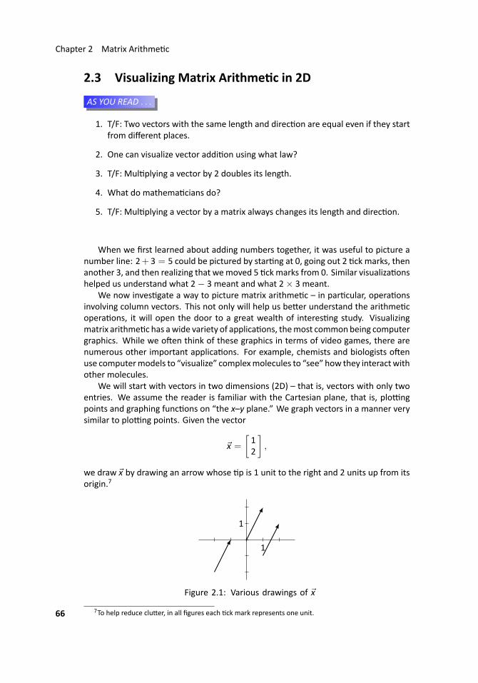
Chapter 2 Matrix Arithme c
2.3 Visualizing Matrix Arithme c in 2D
...AS YOU READ . . .
1. T/F: Two vectors with the same length and direc on are equal even if they startfrom different places.
2. One can visualize vector addi on using what law?
3. T/F: Mul plying a vector by 2 doubles its length.
4. What do mathema cians do?
5. T/F: Mul plying a vector by a matrix always changes its length and direc on.
When we first learned about adding numbers together, it was useful to picture anumber line: 2+ 3 = 5 could be pictured by star ng at 0, going out 2 ck marks, thenanother 3, and then realizing that wemoved 5 ckmarks from 0. Similar visualiza onshelped us understand what 2− 3 meant and what 2× 3 meant.
We now inves gate a way to picture matrix arithme c – in par cular, opera onsinvolving column vectors. This not only will help us be er understand the arithme copera ons, it will open the door to a great wealth of interes ng study. Visualizingmatrix arithme c has awide variety of applica ons, themost commonbeing computergraphics. While we o en think of these graphics in terms of video games, there arenumerous other important applica ons. For example, chemists and biologists o enuse computermodels to “visualize” complexmolecules to “see” how they interactwithother molecules.
We will start with vectors in two dimensions (2D) – that is, vectors with only twoentries. We assume the reader is familiar with the Cartesian plane, that is, plo ngpoints and graphing func ons on “the x–y plane.” We graph vectors in a manner verysimilar to plo ng points. Given the vector
x =
[12
],
we draw x by drawing an arrow whose p is 1 unit to the right and 2 units up from itsorigin.7
..1
.1
..Figure 2.1: Various drawings of x
7To help reduce clu er, in all figures each ck mark represents one unit.66
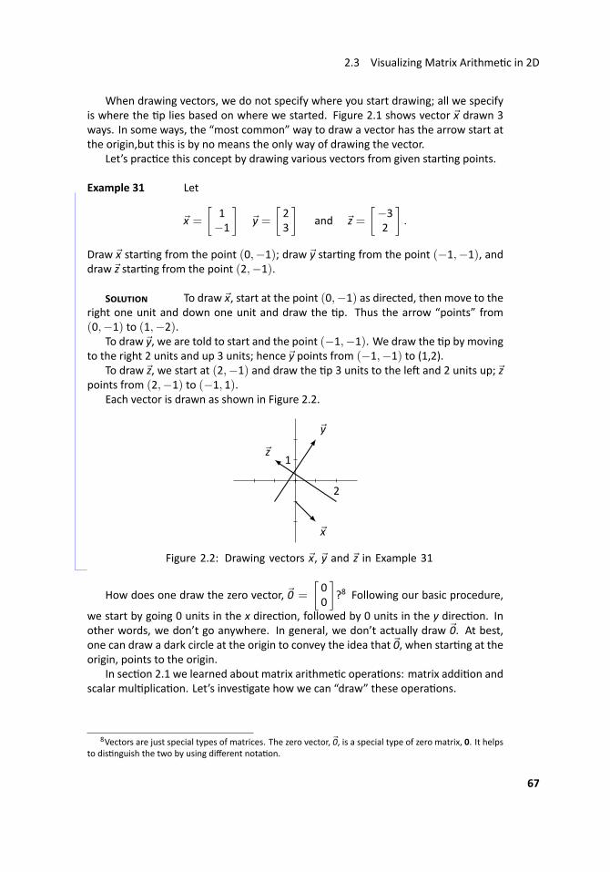
2.3 Visualizing Matrix Arithme c in 2D
When drawing vectors, we do not specify where you start drawing; all we specifyis where the p lies based on where we started. Figure 2.1 shows vector x drawn 3ways. In some ways, the “most common” way to draw a vector has the arrow start atthe origin,but this is by no means the only way of drawing the vector.
Let’s prac ce this concept by drawing various vectors from given star ng points.
.. Example 31 Let
x =
[1−1
]y =
[23
]and z =
[−32
].
Draw x star ng from the point (0,−1); draw y star ng from the point (−1,−1), anddraw z star ng from the point (2,−1).
S To draw x, start at the point (0,−1) as directed, then move to theright one unit and down one unit and draw the p. Thus the arrow “points” from(0,−1) to (1,−2).
To draw y, we are told to start and the point (−1,−1). We draw the p by movingto the right 2 units and up 3 units; hence y points from (−1,−1) to (1,2).
To draw z, we start at (2,−1) and draw the p 3 units to the le and 2 units up; zpoints from (2,−1) to (−1, 1).
Each vector is drawn as shown in Figure 2.2.
..2
.1.
x
.
y
.
z
..Figure 2.2: Drawing vectors x, y and z in Example 31..
How does one draw the zero vector, 0 =
[00
]?8 Following our basic procedure,
we start by going 0 units in the x direc on, followed by 0 units in the y direc on. Inother words, we don’t go anywhere. In general, we don’t actually draw 0. At best,one can draw a dark circle at the origin to convey the idea that 0, when star ng at theorigin, points to the origin.
In sec on 2.1 we learned about matrix arithme c opera ons: matrix addi on andscalar mul plica on. Let’s inves gate how we can “draw” these opera ons.
8Vectors are just special types of matrices. The zero vector, 0, is a special type of zero matrix, 0. It helpsto dis nguish the two by using different nota on.
67
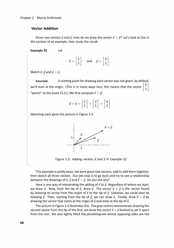
Chapter 2 Matrix Arithme c
Vector Addi on
Given two vectors x and y, how do we draw the vector x + y? Let’s look at this inthe context of an example, then study the result.
.. Example 32 Let
x =
[11
]and y =
[31
].
Sketch x, y and x + y.
S A star ng point for drawing each vector was not given; by default,
we’ll start at the origin. (This is in many ways nice; this means that the vector[31
]“points” to the point (3,1).) We first compute x + y:
x + y =[11
]+
[31
]=
[42
]Sketching each gives the picture in Figure 2.3.
..1
.
1
.
x
.y
.
x + y
..Figure 2.3: Adding vectors x and y in Example 32..
This example is pre y basic; wewere given two vectors, told to add them together,then sketch all three vectors. Our job now is to go back and try to see a rela onshipbetween the drawings of x, y and x + y. Do you see any?
Here is one way of interpre ng the adding of x to y. Regardless of where we start,we draw x. Now, from the p of x, draw y. The vector x + y is the vector foundby drawing an arrow from the origin of x to the p of y. Likewise, we could start bydrawing y. Then, star ng from the p of y, we can draw x. Finally, draw x + y bydrawing the vector that starts at the origin of y and ends at the p of x.
The picture in Figure 2.4 illustrates this. The gray vectors demonstrate drawing thesecond vector from the p of the first; we draw the vector x + y dashed to set it apartfrom the rest. We also lightly filled the parallelogram whose opposing sides are the
68
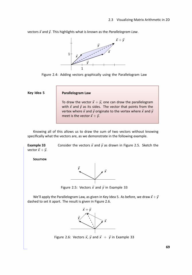
2.3 Visualizing Matrix Arithme c in 2D
vectors x and y. This highlights what is known as the Parallelogram Law.
..1
.
1
.
x
. y.
x
.
y
.
x + y
..Figure 2.4: Adding vectors graphically using the Parallelogram Law
..Key Idea 5
.
.Parallelogram Law
To draw the vector x + y, one can draw the parallelogramwith x and y as its sides. The vector that points from thevertex where x and y originate to the vertex where x and ymeet is the vector x + y.
Knowing all of this allows us to draw the sum of two vectors without knowingspecifically what the vectors are, as we demonstrate in the following example.
.. Example 33 Consider the vectors x and y as drawn in Figure 2.5. Sketch thevector x + y.
S
..
x
.
y
..Figure 2.5: Vectors x and y in Example 33
We’ll apply the Parallelogram Law, as given in Key Idea 5. As before, we draw x+ ydashed to set it apart. The result is given in Figure 2.6.
..
x
.
y
.
x + y
..Figure 2.6: Vectors x, y and x + y in Example 33
.. 69
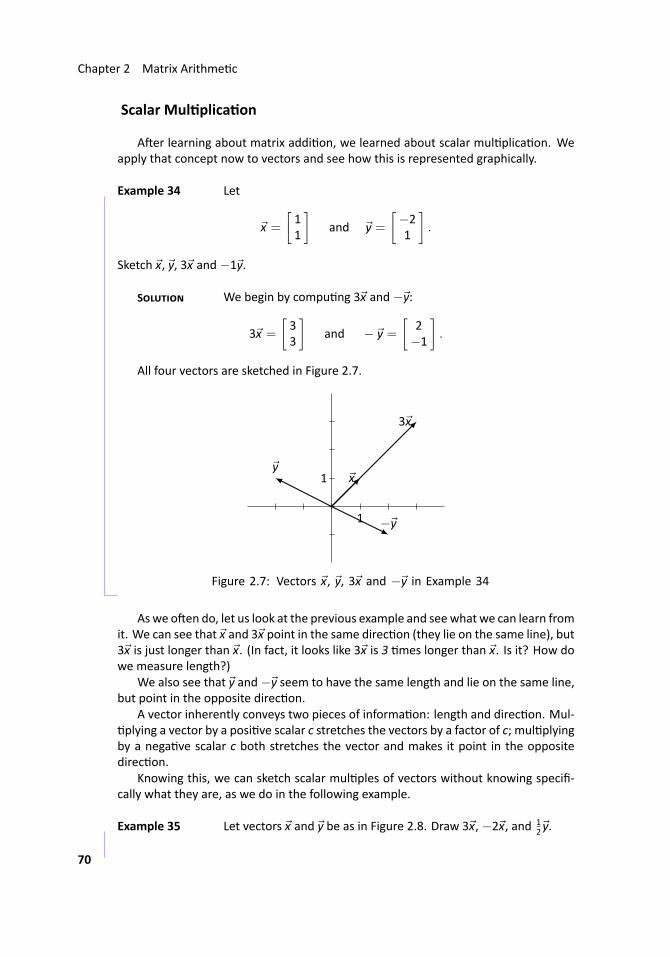
Chapter 2 Matrix Arithme c
Scalar Mul plica on
A er learning about matrix addi on, we learned about scalar mul plica on. Weapply that concept now to vectors and see how this is represented graphically.
.. Example 34 Let
x =
[11
]and y =
[−21
].
Sketch x, y, 3x and−1y.
S We begin by compu ng 3x and−y:
3x =
[33
]and − y =
[2−1
].
All four vectors are sketched in Figure 2.7.
..1
.
1
.
3x
.
x
.
y
.
−y
..Figure 2.7: Vectors x, y, 3x and −y in Example 34..
As we o en do, let us look at the previous example and seewhat we can learn fromit. We can see that x and 3x point in the same direc on (they lie on the same line), but3x is just longer than x. (In fact, it looks like 3x is 3 mes longer than x. Is it? How dowe measure length?)
We also see that y and−y seem to have the same length and lie on the same line,but point in the opposite direc on.
A vector inherently conveys two pieces of informa on: length and direc on. Mul-plying a vector by a posi ve scalar c stretches the vectors by a factor of c; mul plying
by a nega ve scalar c both stretches the vector and makes it point in the oppositedirec on.
Knowing this, we can sketch scalar mul ples of vectors without knowing specifi-cally what they are, as we do in the following example.
.. Example 35 ..Let vectors x and y be as in Figure 2.8. Draw 3x,−2x, and 12 y.
70
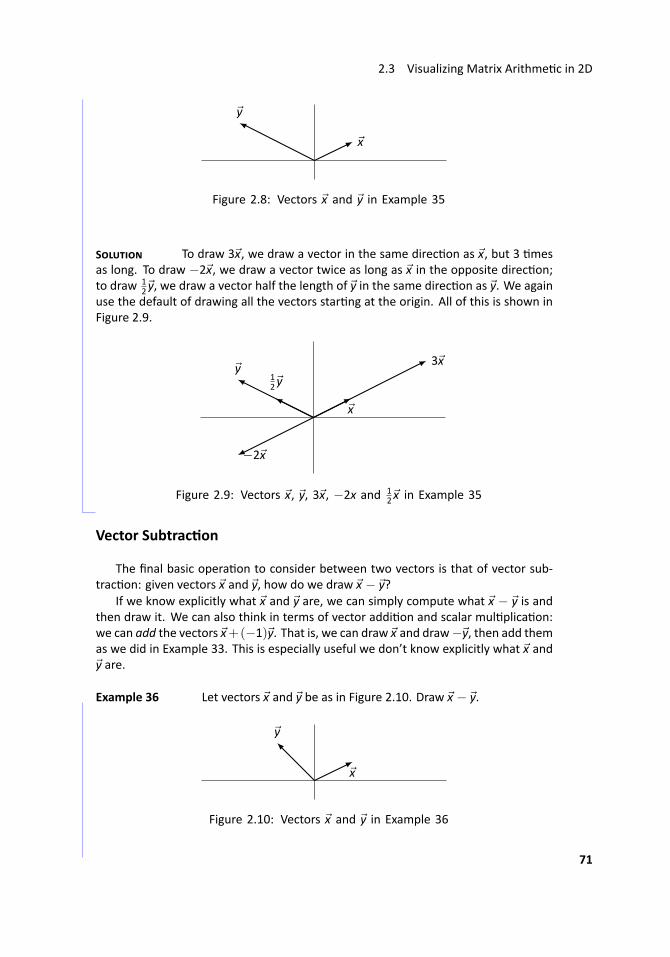
2.3 Visualizing Matrix Arithme c in 2D
..x
.
y
..Figure 2.8: Vectors x and y in Example 35
S To draw 3x, we draw a vector in the same direc on as x, but 3 mesas long. To draw −2x, we draw a vector twice as long as x in the opposite direc on;to draw 1
2 y, we draw a vector half the length of y in the same direc on as y. We againuse the default of drawing all the vectors star ng at the origin. All of this is shown inFigure 2.9.
.. x.
y
.
3x
.
−2x
.
12 y
..Figure 2.9: Vectors x, y, 3x, −2x and 12 x in Example 35
...
Vector Subtrac on
The final basic opera on to consider between two vectors is that of vector sub-trac on: given vectors x and y, how do we draw x − y?
If we know explicitly what x and y are, we can simply compute what x − y is andthen draw it. We can also think in terms of vector addi on and scalar mul plica on:we can add the vectors x+(−1)y. That is, we can draw x and draw−y, then add themas we did in Example 33. This is especially useful we don’t know explicitly what x andy are.
.. Example 36 ..Let vectors x and y be as in Figure 2.10. Draw x − y.
.. x.
y
..Figure 2.10: Vectors x and y in Example 36
71
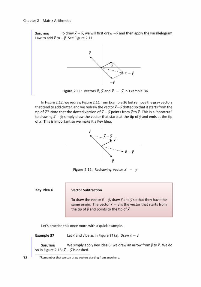
Chapter 2 Matrix Arithme c
S To draw x − y, we will first draw−y and then apply the ParallelogramLaw to add x to−y. See Figure 2.11.
.. x.
y
.
−y
.
x − y
..Figure 2.11: Vectors x, y and x − y in Example 36...
In Figure 2.12, we redraw Figure 2.11 from Example 36 but remove the gray vectorsthat tend to add clu er, andwe redraw the vector x− y do ed so that it starts from thep of y.9 Note that the do ed version of x − y points from y to x. This is a “shortcut”
to drawing x − y; simply draw the vector that starts at the p of y and ends at the pof x. This is important so we make it a Key Idea.
..x
.
y
.
-y
.
x − y
.
x − y
..Figure 2.12: Redrawing vector x − y
..Key Idea 6
.
.Vector Subtrac on
To draw the vector x− y, draw x and y so that they have thesame origin. The vector x − y is the vector that starts fromthe p of y and points to the p of x.
Let’s prac ce this once more with a quick example.
.. Example 37 ..Let x and y be as in Figure ?? (a). Draw x − y.
S We simply apply Key Idea 6: we draw an arrow from y to x. We doso in Figure 2.13; x − y is dashed.
9Remember that we can draw vectors star ng from anywhere.72
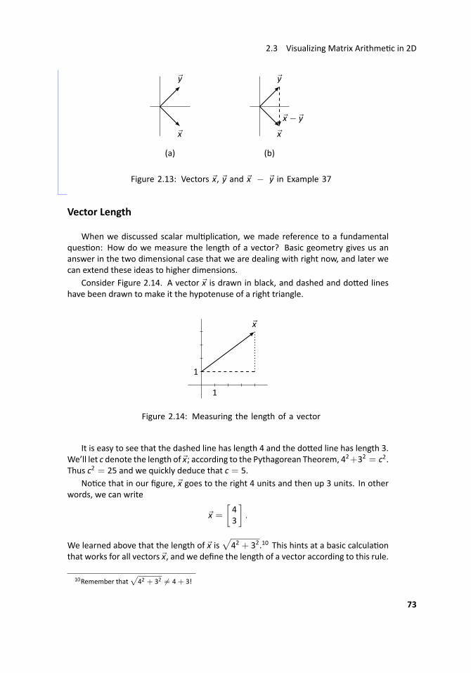
2.3 Visualizing Matrix Arithme c in 2D
..
y
.
x
.
(a)
.
y
.
x
.
x − y
.
(b)
..Figure 2.13: Vectors x, y and x − y in Example 37...
Vector Length
When we discussed scalar mul plica on, we made reference to a fundamentalques on: How do we measure the length of a vector? Basic geometry gives us ananswer in the two dimensional case that we are dealing with right now, and later wecan extend these ideas to higher dimensions.
Consider Figure 2.14. A vector x is drawn in black, and dashed and do ed lineshave been drawn to make it the hypotenuse of a right triangle.
..1
.1.
x
..Figure 2.14: Measuring the length of a vector
It is easy to see that the dashed line has length 4 and the do ed line has length 3.We’ll let c denote the length of x; according to the Pythagorean Theorem, 42+32 = c2.Thus c2 = 25 and we quickly deduce that c = 5.
No ce that in our figure, x goes to the right 4 units and then up 3 units. In otherwords, we can write
x =
[43
].
We learned above that the length of x is√
42 + 32.10 This hints at a basic calcula onthat works for all vectors x, and we define the length of a vector according to this rule.
10Remember that√
42 + 32 = 4+ 3!
73
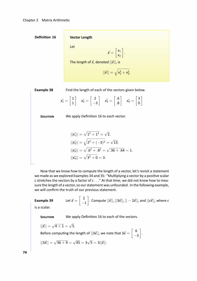
Chapter 2 Matrix Arithme c
..Defini on 16
.
.Vector Length
Let
x =
[x1x2
].
The length of x, denoted ||x||, is
||x|| =√
x21 + x22.
.. Example 38 Find the length of each of the vectors given below.
x1 =[11
]x2 =
[2−3
]x3 =
[.6.8
]x4 =
[30
]
S We apply Defini on 16 to each vector.
||x1|| =√
12 + 12 =√2.
||x2|| =√
22 + (−3)2 =√13.
||x3|| =√.62 + .82 =
√.36+ .64 = 1.
||x4|| =√
32 + 0 = 3...
Now that we know how to compute the length of a vector, let’s revisit a statementwemade aswe explored Examples 34 and 35: “Mul plying a vector by a posi ve scalarc stretches the vectors by a factor of c . . .” At that me, we did not know how to mea-sure the length of a vector, so our statementwas unfounded. In the following example,we will confirm the truth of our previous statement.
.. Example 39 ..Let x =
[2−1
]. Compute ||x||, ||3x||, || − 2x||, and ||cx||, where c
is a scalar.
S We apply Defini on 16 to each of the vectors.
||x|| =√4+ 1 =
√5.
Before compu ng the length of ||3x||, we note that 3x =
[6−3
].
||3x|| =√36+ 9 =
√45 = 3
√5 = 3||x||.
74
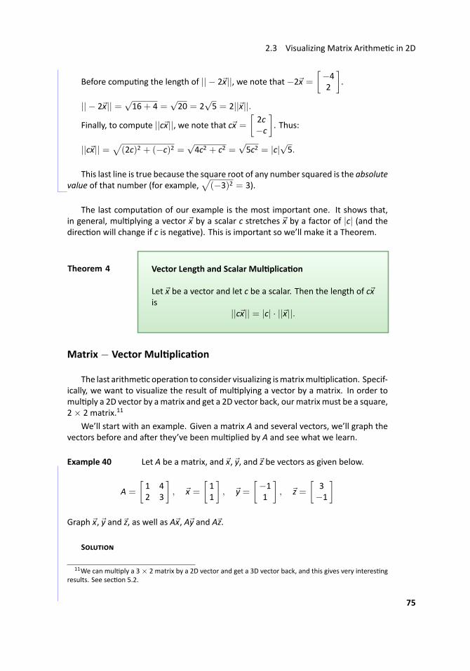
2.3 Visualizing Matrix Arithme c in 2D
Before compu ng the length of || − 2x||, we note that−2x =
[−42
].
|| − 2x|| =√16+ 4 =
√20 = 2
√5 = 2||x||.
Finally, to compute ||cx||, we note that cx =
[2c−c
]. Thus:
||cx|| =√
(2c)2 + (−c)2 =√4c2 + c2 =
√5c2 = |c|
√5.
This last line is true because the square root of any number squared is the absolutevalue of that number (for example,
√(−3)2 = 3). ...
The last computa on of our example is the most important one. It shows that,in general, mul plying a vector x by a scalar c stretches x by a factor of |c| (and thedirec on will change if c is nega ve). This is important so we’ll make it a Theorem.
..Theorem 4
.
.Vector Length and Scalar Mul plica on
Let x be a vector and let c be a scalar. Then the length of cxis
||cx|| = |c| · ||x||.
Matrix− Vector Mul plica on
The last arithme copera on to consider visualizing ismatrixmul plica on. Specif-ically, we want to visualize the result of mul plying a vector by a matrix. In order tomul ply a 2D vector by amatrix and get a 2D vector back, ourmatrix must be a square,2× 2 matrix.11
We’ll start with an example. Given a matrix A and several vectors, we’ll graph thevectors before and a er they’ve been mul plied by A and see what we learn.
.. Example 40 ..Let A be a matrix, and x, y, and z be vectors as given below.
A =
[1 42 3
], x =
[11
], y =
[−11
], z =
[3−1
]
Graph x, y and z, as well as Ax, Ay and Az.
S
11We can mul ply a 3× 2 matrix by a 2D vector and get a 3D vector back, and this gives very interes ngresults. See sec on 5.2.
75
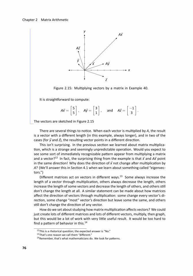
Chapter 2 Matrix Arithme c
.. x.
y
.x
.
y
.
z
.
Ax
.Ay
.
Az
..Figure 2.15: Mul plying vectors by a matrix in Example 40.
It is straigh orward to compute:
Ax =
[55
], Ay =
[31
], and Az =
[−13
].
The vectors are sketched in Figure 2.15 ...
There are several things to no ce. When each vector is mul plied by A, the resultis a vector with a different length (in this example, always longer), and in two of thecases (for y and z), the resul ng vector points in a different direc on.
This isn’t surprising. In the previous sec on we learned about matrix mul plica-on, which is a strange and seemingly unpredictable opera on. Would you expect to
see some sort of immediately recognizable pa ern appear from mul plying a matrixand a vector?12 In fact, the surprising thing from the example is that x and Ax pointin the same direc on! Why does the direc on of x not change a er mul plica on byA? (We’ll answer this in Sec on 4.1 when we learn about something called “eigenvec-tors.”)
Different matrices act on vectors in different ways.13 Some always increase thelength of a vector through mul plica on, others always decrease the length, othersincrease the length of some vectors and decrease the length of others, and others s lldon’t change the length at all. A similar statement can be made about how matricesaffect the direc on of vectors through mul plica on: some change every vector’s di-rec on, some change “most” vector’s direc on but leave some the same, and otherss ll don’t change the direc on of any vector.
How dowe set about studying howmatrixmul plica on affects vectors? We couldjust create lots of different matrices and lots of different vectors, mul ply, then graph,but this would be a lot of work with very li le useful result. It would be too hard tofind a pa ern of behavior in this.14
12This is a rhetorical ques on; the expected answer is “No.”13That’s one reason we call them “different.”14Remember, that’s what mathema cians do. We look for pa erns.
76
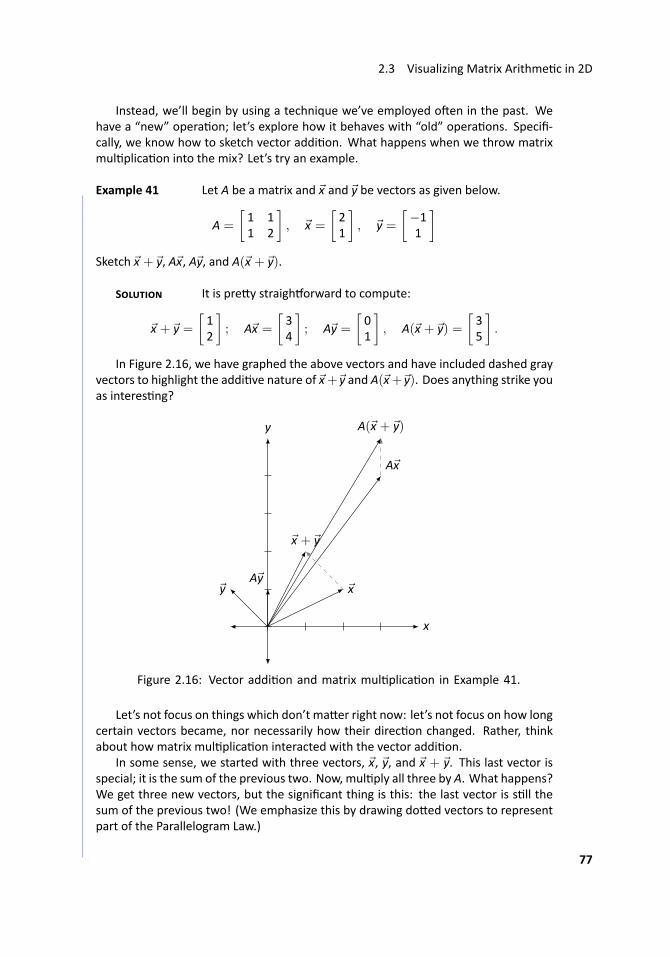
2.3 Visualizing Matrix Arithme c in 2D
Instead, we’ll begin by using a technique we’ve employed o en in the past. Wehave a “new” opera on; let’s explore how it behaves with “old” opera ons. Specifi-cally, we know how to sketch vector addi on. What happens when we throw matrixmul plica on into the mix? Let’s try an example.
.. Example 41 ..Let A be a matrix and x and y be vectors as given below.
A =
[1 11 2
], x =
[21
], y =
[−11
]Sketch x + y, Ax, Ay, and A(x + y).
S It is pre y straigh orward to compute:
x + y =[12
]; Ax =
[34
]; Ay =
[01
], A(x + y) =
[35
].
In Figure 2.16, we have graphed the above vectors and have included dashed grayvectors to highlight the addi ve nature of x+ y and A(x+ y). Does anything strike youas interes ng?
.. x.
y
.
x
.
y
.
x + y
.
Ax
.
Ay
.
A(x + y)
..Figure 2.16: Vector addi on and matrix mul plica on in Example 41.
Let’s not focus on things which don’t ma er right now: let’s not focus on how longcertain vectors became, nor necessarily how their direc on changed. Rather, thinkabout how matrix mul plica on interacted with the vector addi on.
In some sense, we started with three vectors, x, y, and x + y. This last vector isspecial; it is the sum of the previous two. Now, mul ply all three by A. What happens?We get three new vectors, but the significant thing is this: the last vector is s ll thesum of the previous two! (We emphasize this by drawing do ed vectors to representpart of the Parallelogram Law.)
77
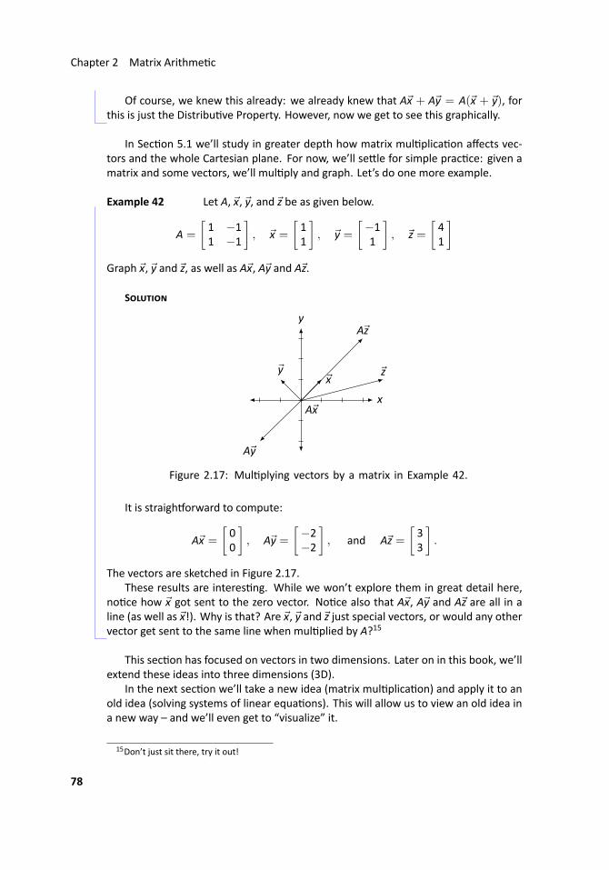
Chapter 2 Matrix Arithme c
Of course, we knew this already: we already knew that Ax + Ay = A(x + y), forthis is just the Distribu ve Property. However, now we get to see this graphically. ...
In Sec on 5.1 we’ll study in greater depth how matrix mul plica on affects vec-tors and the whole Cartesian plane. For now, we’ll se le for simple prac ce: given amatrix and some vectors, we’ll mul ply and graph. Let’s do one more example.
.. Example 42 Let A, x, y, and z be as given below.
A =
[1 −11 −1
], x =
[11
], y =
[−11
], z =
[41
]Graph x, y and z, as well as Ax, Ay and Az.
S
.. x.
y
.x
.
y
.
z
.Ax.
Ay
.
Az
..Figure 2.17: Mul plying vectors by a matrix in Example 42.
It is straigh orward to compute:
Ax =
[00
], Ay =
[−2−2
], and Az =
[33
].
The vectors are sketched in Figure 2.17.These results are interes ng. While we won’t explore them in great detail here,
no ce how x got sent to the zero vector. No ce also that Ax, Ay and Az are all in aline (as well as x!). Why is that? Are x, y and z just special vectors, or would any othervector get sent to the same line when mul plied by A?15 ..
This sec on has focused on vectors in two dimensions. Later on in this book, we’llextend these ideas into three dimensions (3D).
In the next sec on we’ll take a new idea (matrix mul plica on) and apply it to anold idea (solving systems of linear equa ons). This will allow us to view an old idea ina new way – and we’ll even get to “visualize” it.
15Don’t just sit there, try it out!
78
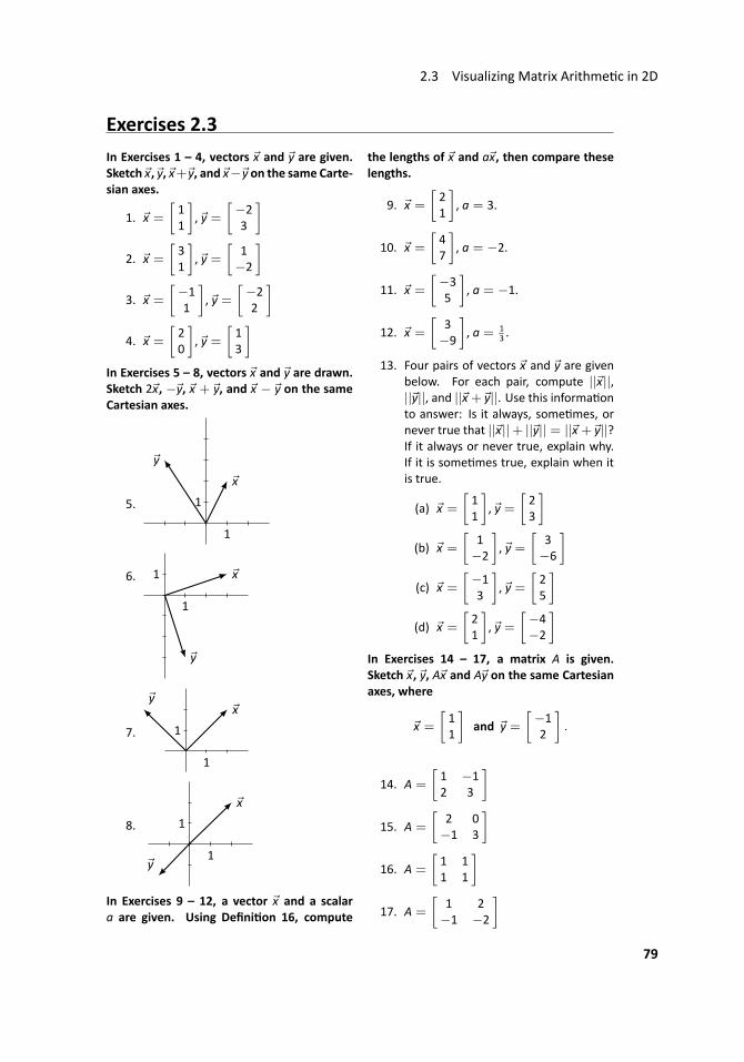
2.3 Visualizing Matrix Arithme c in 2D
Exercises 2.3In Exercises 1 – 4, vectors x and y are given.Sketch x, y, x+ y, and x− y on the same Carte-sian axes.
1. x =
[11
], y =
[−23
]2. x =
[31
], y =
[1−2
]3. x =
[−11
], y =
[−22
]4. x =
[20
], y =
[13
]In Exercises 5 – 8, vectors x and y are drawn.Sketch 2x, −y, x + y, and x − y on the sameCartesian axes.
5...
1.
1.
x
.
y
6...
1.
1.
x.
y
7...
1.
1.
x
.
y
8...
1.
1.
x
.
y
In Exercises 9 – 12, a vector x and a scalara are given. Using Defini on 16, compute
the lengths of x and ax, then compare theselengths.
9. x =
[21
], a = 3.
10. x =
[47
], a = −2.
11. x =
[−35
], a = −1.
12. x =
[3−9
], a = 1
3 .
13. Four pairs of vectors x and y are givenbelow. For each pair, compute ||x||,||y||, and ||x + y||. Use this informa onto answer: Is it always, some mes, ornever true that ||x||+ ||y|| = ||x + y||?If it always or never true, explain why.If it is some mes true, explain when itis true.
(a) x =
[11
], y =
[23
](b) x =
[1−2
], y =
[3−6
](c) x =
[−13
], y =
[25
](d) x =
[21
], y =
[−4−2
]In Exercises 14 – 17, a matrix A is given.Sketch x, y, Ax and Ay on the same Cartesianaxes, where
x =
[11
]and y =
[−12
].
14. A =
[1 −12 3
]15. A =
[2 0−1 3
]16. A =
[1 11 1
]17. A =
[1 2−1 −2
]79
Chapter 2 Matrix Arithme c
2.4 Vector Solu ons to Linear Systems
...AS YOU READ . . .
1. T/F: The equa on Ax = b is just another way of wri ng a system of linear equa-ons.
2. T/F: In solving Ax = 0, if there are 3 free variables, then the solu on will be“pulled apart” into 3 vectors.
3. T/F: A homogeneous system of linear equa ons is one in which all of the coeffi-cients are 0.
4. Whether or not the equa on Ax = b has a solu on depends on an intrinsicproperty of .
The first chapter of this text was spent finding solu ons to systems of linear equa-ons. We have spent the first two sec ons of this chapter learning opera ons that
can be performed with matrices. One may have wondered “Are the ideas of the firstchapter related to what we have been doing recently?” The answer is yes, these ideasare related. This sec on begins to show that rela onship.
We have o en hearkened back to previous algebra experience to help understandmatrix algebra concepts. We do that again here. Consider the equa on ax = b, wherea = 3 and b = 6. If we asked one to “solve for x,” what exactly would we be asking?We would want to find a number, which we call x, where a mes x gives b; in this case,it is a number, when mul plied by 3, returns 6.
Now we consider matrix algebra expressions. We’ll eventually consider solvingequa ons like AX = B, where we know what the matrices A and B are and we want tofind the matrix X. For now, we’ll only consider equa ons of the type Ax = b, wherewe know the matrix A and the vector b. We will want to find what vector x sa sfiesthis equa on; we want to “solve for x.”
To help understand what this is asking, we’ll consider an example. Let
A =
1 1 11 −1 22 0 1
, b =
2−31
and x =
x1x2x3
.
(We don’t know what x is, so we have to represent it’s entries with the variables x1, x2and x3.) Let’s “solve for x,” given the equa on Ax = b.
We can mul ply out the le hand side of this equa on. We find that
Ax =
x1 + x2 + x3x1 − x2 + 2x3
2x1 + x3
.
Be sure to note that the product is just a vector; it has just one column.
80
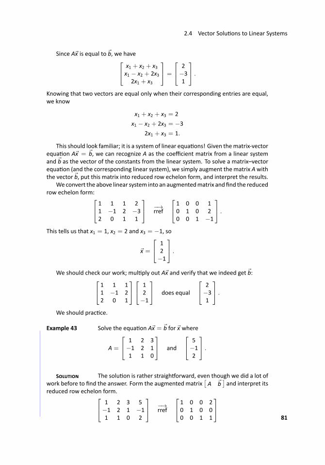
2.4 Vector Solu ons to Linear Systems
Since Ax is equal to b, we have x1 + x2 + x3x1 − x2 + 2x3
2x1 + x3
=
2−31
.
Knowing that two vectors are equal only when their corresponding entries are equal,we know
x1 + x2 + x3 = 2
x1 − x2 + 2x3 = −3
2x1 + x3 = 1.
This should look familiar; it is a system of linear equa ons! Given thematrix-vectorequa on Ax = b, we can recognize A as the coefficient matrix from a linear systemand b as the vector of the constants from the linear system. To solve a matrix–vectorequa on (and the corresponding linear system), we simply augment the matrix Awiththe vector b, put this matrix into reduced row echelon form, and interpret the results.
We convert the above linear system into an augmentedmatrix andfind the reducedrow echelon form: 1 1 1 2
1 −1 2 −32 0 1 1
−→rref
1 0 0 10 1 0 20 0 1 −1
.
This tells us that x1 = 1, x2 = 2 and x3 = −1, so
x =
12−1
.
We should check our work; mul ply out Ax and verify that we indeed get b: 1 1 11 −1 22 0 1
12−1
does equal
2−31
.
We should prac ce.
.. Example 43 ..Solve the equa on Ax = b for x where
A =
1 2 3−1 2 11 1 0
and
5−12
.
S The solu on is rather straigh orward, even though we did a lot ofwork before to find the answer. Form the augmented matrix
[A b
]and interpret its
reduced row echelon form. 1 2 3 5−1 2 1 −11 1 0 2
−→rref
1 0 0 20 1 0 00 0 1 1
81
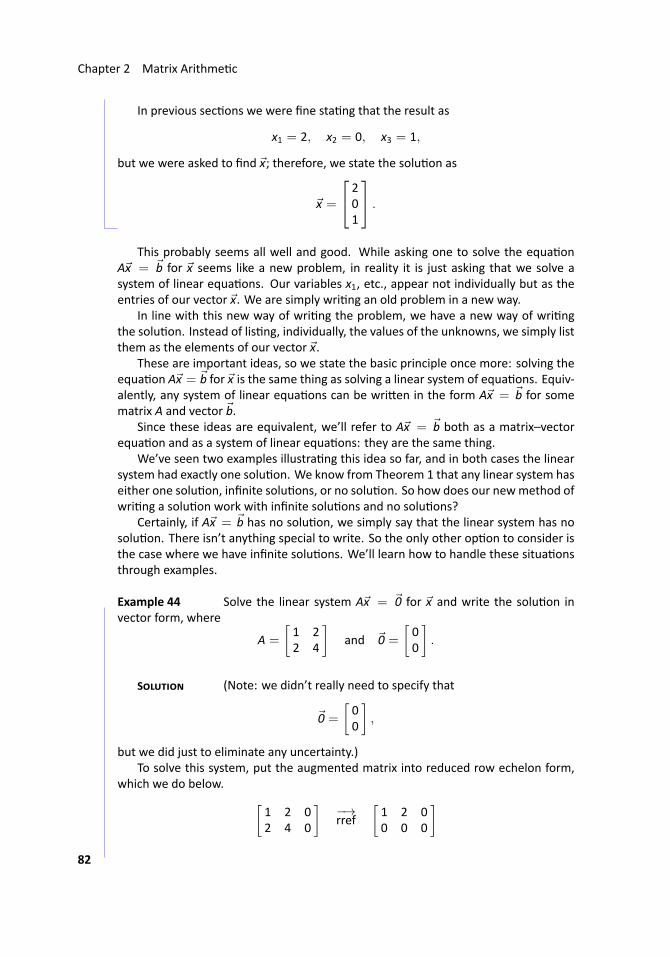
Chapter 2 Matrix Arithme c
In previous sec ons we were fine sta ng that the result as
x1 = 2, x2 = 0, x3 = 1,
but we were asked to find x; therefore, we state the solu on as
x =
201
....
This probably seems all well and good. While asking one to solve the equa onAx = b for x seems like a new problem, in reality it is just asking that we solve asystem of linear equa ons. Our variables x1, etc., appear not individually but as theentries of our vector x. We are simply wri ng an old problem in a new way.
In line with this new way of wri ng the problem, we have a new way of wri ngthe solu on. Instead of lis ng, individually, the values of the unknowns, we simply listthem as the elements of our vector x.
These are important ideas, so we state the basic principle once more: solving theequa on Ax = b for x is the same thing as solving a linear system of equa ons. Equiv-alently, any system of linear equa ons can be wri en in the form Ax = b for somematrix A and vector b.
Since these ideas are equivalent, we’ll refer to Ax = b both as a matrix–vectorequa on and as a system of linear equa ons: they are the same thing.
We’ve seen two examples illustra ng this idea so far, and in both cases the linearsystem had exactly one solu on. We know from Theorem 1 that any linear system haseither one solu on, infinite solu ons, or no solu on. So how does our newmethod ofwri ng a solu on work with infinite solu ons and no solu ons?
Certainly, if Ax = b has no solu on, we simply say that the linear system has nosolu on. There isn’t anything special to write. So the only other op on to consider isthe case where we have infinite solu ons. We’ll learn how to handle these situa onsthrough examples.
.. Example 44 ..Solve the linear system Ax = 0 for x and write the solu on invector form, where
A =
[1 22 4
]and 0 =
[00
].
S (Note: we didn’t really need to specify that
0 =
[00
],
but we did just to eliminate any uncertainty.)To solve this system, put the augmented matrix into reduced row echelon form,
which we do below. [1 2 02 4 0
]−→rref
[1 2 00 0 0
]82
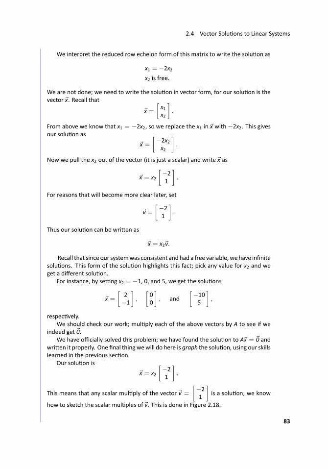
2.4 Vector Solu ons to Linear Systems
We interpret the reduced row echelon form of this matrix to write the solu on as
x1 = −2x2x2 is free.
We are not done; we need to write the solu on in vector form, for our solu on is thevector x. Recall that
x =
[x1x2
].
From above we know that x1 = −2x2, so we replace the x1 in x with −2x2. This givesour solu on as
x =
[−2x2x2
].
Now we pull the x2 out of the vector (it is just a scalar) and write x as
x = x2
[−21
].
For reasons that will become more clear later, set
v =[−21
].
Thus our solu on can be wri en as
x = x2v.
..Recall that since our systemwas consistent and had a free variable, wehave infinitesolu ons. This form of the solu on highlights this fact; pick any value for x2 and weget a different solu on.
For instance, by se ng x2 = −1, 0, and 5, we get the solu ons
x =
[2−1
],
[00
], and
[−105
],
respec vely.We should check our work; mul ply each of the above vectors by A to see if we
indeed get 0.We have officially solved this problem; we have found the solu on to Ax = 0 and
wri en it properly. One final thing wewill do here is graph the solu on, using our skillslearned in the previous sec on.
Our solu on is
x = x2
[−21
].
This means that any scalar mul ply of the vector v =
[−21
]is a solu on; we know
how to sketch the scalar mul ples of v. This is done in Figure 2.18.
83
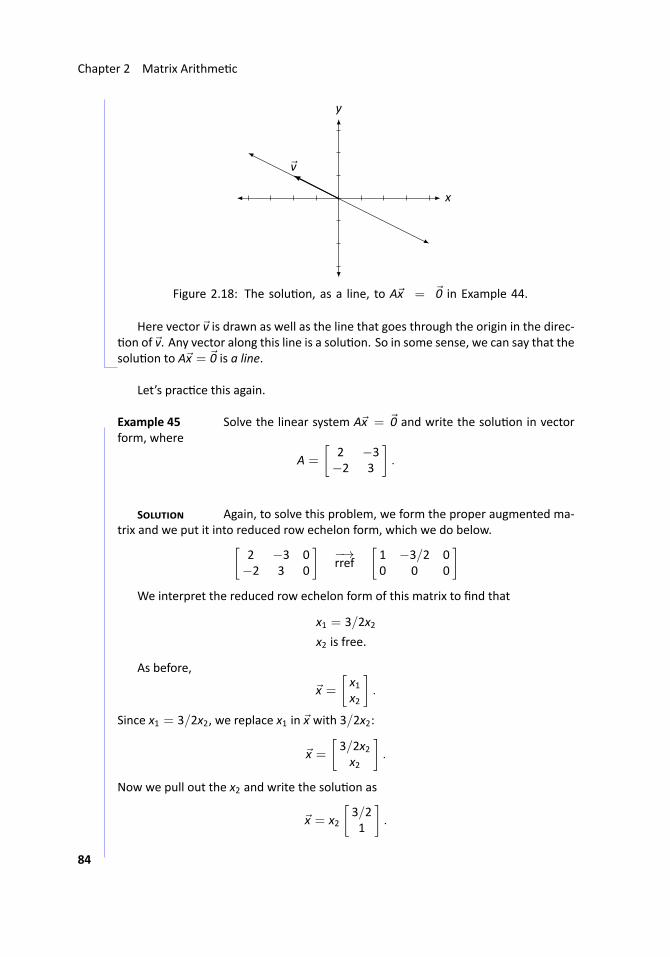
Chapter 2 Matrix Arithme c
.. x.
y
.
v
..Figure 2.18: The solu on, as a line, to Ax = 0 in Example 44.
Here vector v is drawn as well as the line that goes through the origin in the direc-on of v. Any vector along this line is a solu on. So in some sense, we can say that the
solu on to Ax = 0 is a line. ...
Let’s prac ce this again.
.. Example 45 ..Solve the linear system Ax = 0 and write the solu on in vectorform, where
A =
[2 −3−2 3
].
S Again, to solve this problem, we form the proper augmented ma-trix and we put it into reduced row echelon form, which we do below.[
2 −3 0−2 3 0
]−→rref
[1 −3/2 00 0 0
]We interpret the reduced row echelon form of this matrix to find that
x1 = 3/2x2x2 is free.
As before,
x =
[x1x2
].
Since x1 = 3/2x2, we replace x1 in x with 3/2x2:
x =
[3/2x2x2
].
Now we pull out the x2 and write the solu on as
x = x2
[3/21
].
84
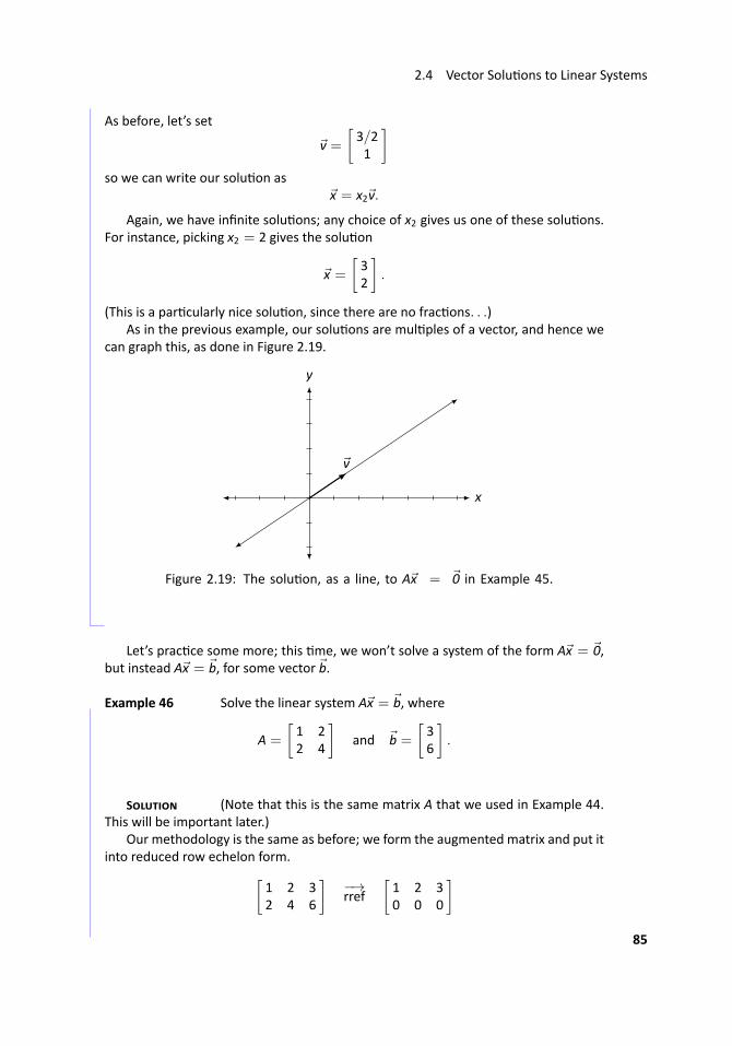
2.4 Vector Solu ons to Linear Systems
As before, let’s set
v =[3/21
]so we can write our solu on as
x = x2v.
Again, we have infinite solu ons; any choice of x2 gives us one of these solu ons.For instance, picking x2 = 2 gives the solu on
x =
[32
].
(This is a par cularly nice solu on, since there are no frac ons. . .)As in the previous example, our solu ons are mul ples of a vector, and hence we
can graph this, as done in Figure 2.19.
.. x.
y
.
v
..Figure 2.19: The solu on, as a line, to Ax = 0 in Example 45.
...
Let’s prac ce some more; this me, we won’t solve a system of the form Ax = 0,but instead Ax = b, for some vector b.
.. Example 46 ..Solve the linear system Ax = b, where
A =
[1 22 4
]and b =
[36
].
S (Note that this is the same matrix A that we used in Example 44.This will be important later.)
Our methodology is the same as before; we form the augmented matrix and put itinto reduced row echelon form.[
1 2 32 4 6
]−→rref
[1 2 30 0 0
]85
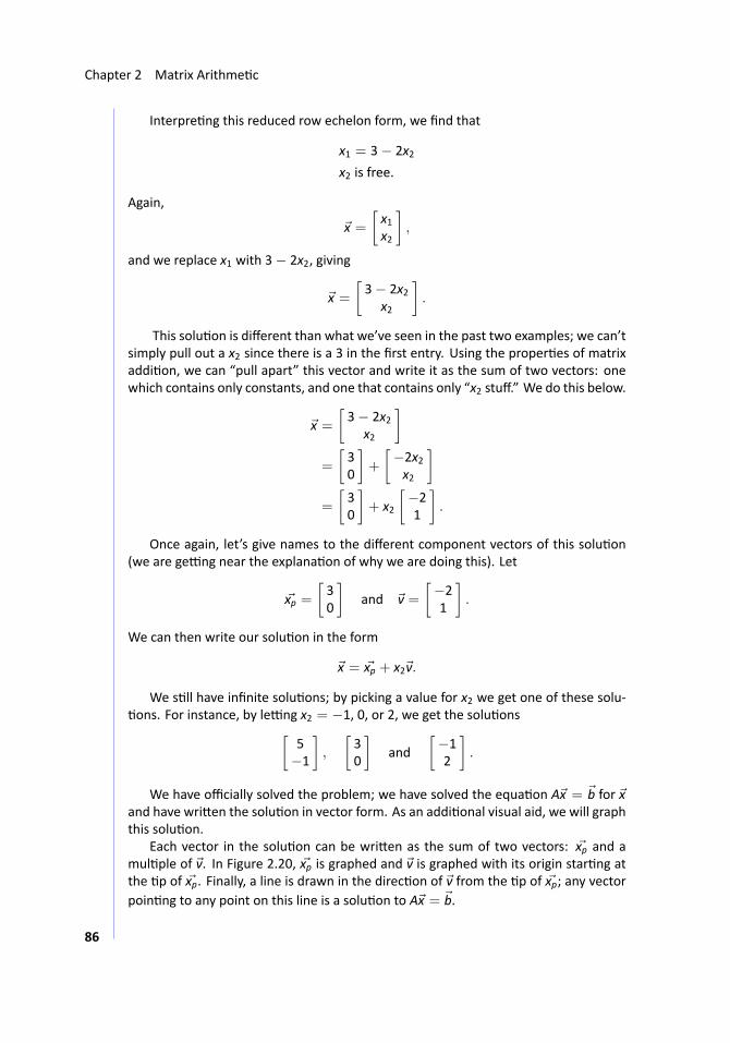
Chapter 2 Matrix Arithme c
Interpre ng this reduced row echelon form, we find that
x1 = 3− 2x2x2 is free.
Again,
x =
[x1x2
],
and we replace x1 with 3− 2x2, giving
x =
[3− 2x2
x2
].
..This solu on is different than what we’ve seen in the past two examples; we can’tsimply pull out a x2 since there is a 3 in the first entry. Using the proper es of matrixaddi on, we can “pull apart” this vector and write it as the sum of two vectors: onewhich contains only constants, and one that contains only “x2 stuff.” We do this below.
x =
[3− 2x2
x2
]=
[30
]+
[−2x2x2
]=
[30
]+ x2
[−21
].
Once again, let’s give names to the different component vectors of this solu on(we are ge ng near the explana on of why we are doing this). Let
xp =[30
]and v =
[−21
].
We can then write our solu on in the form
x = xp + x2v.
We s ll have infinite solu ons; by picking a value for x2 we get one of these solu-ons. For instance, by le ng x2 = −1, 0, or 2, we get the solu ons[
5−1
],
[30
]and
[−12
].
We have officially solved the problem; we have solved the equa on Ax = b for xand have wri en the solu on in vector form. As an addi onal visual aid, we will graphthis solu on.
Each vector in the solu on can be wri en as the sum of two vectors: xp and amul ple of v. In Figure 2.20, xp is graphed and v is graphed with its origin star ng atthe p of xp. Finally, a line is drawn in the direc on of v from the p of xp; any vectorpoin ng to any point on this line is a solu on to Ax = b.
86
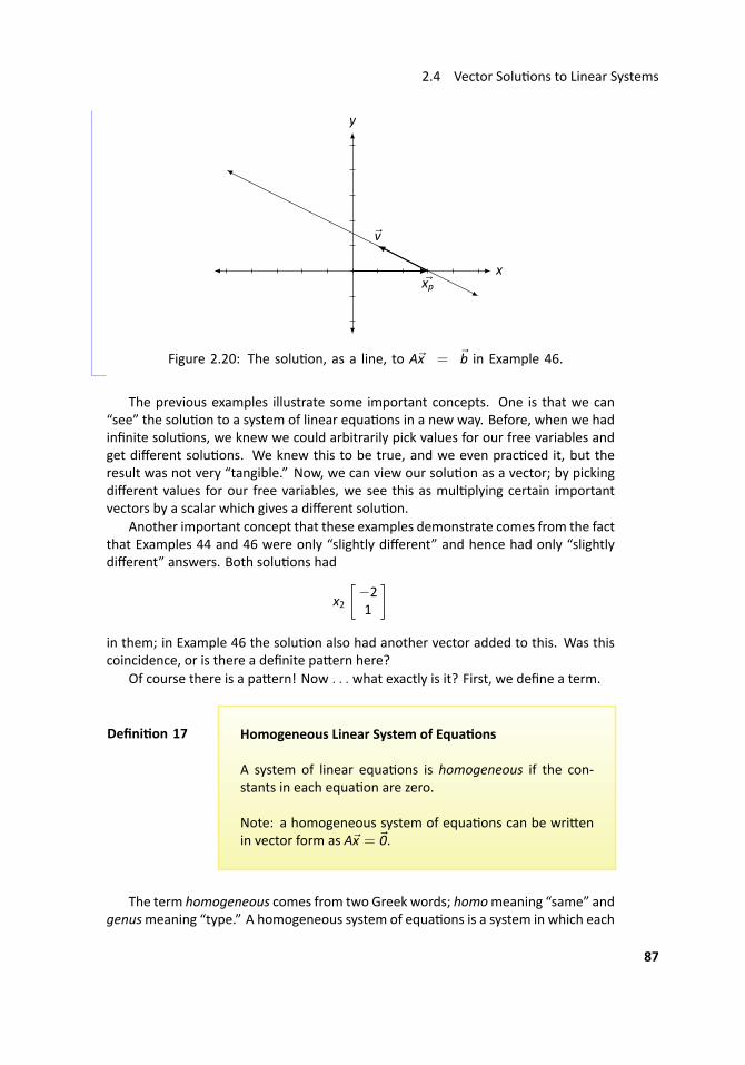
2.4 Vector Solu ons to Linear Systems
.. x.
y
.xp
.
v
..Figure 2.20: The solu on, as a line, to Ax = b in Example 46....
The previous examples illustrate some important concepts. One is that we can“see” the solu on to a system of linear equa ons in a new way. Before, when we hadinfinite solu ons, we knew we could arbitrarily pick values for our free variables andget different solu ons. We knew this to be true, and we even prac ced it, but theresult was not very “tangible.” Now, we can view our solu on as a vector; by pickingdifferent values for our free variables, we see this as mul plying certain importantvectors by a scalar which gives a different solu on.
Another important concept that these examples demonstrate comes from the factthat Examples 44 and 46 were only “slightly different” and hence had only “slightlydifferent” answers. Both solu ons had
x2
[−21
]in them; in Example 46 the solu on also had another vector added to this. Was thiscoincidence, or is there a definite pa ern here?
Of course there is a pa ern! Now . . . what exactly is it? First, we define a term.
..Defini on 17
.
.Homogeneous Linear System of Equa ons
A system of linear equa ons is homogeneous if the con-stants in each equa on are zero.
Note: a homogeneous system of equa ons can be wri enin vector form as Ax = 0.
The term homogeneous comes from two Greek words; homomeaning “same” andgenusmeaning “type.” A homogeneous system of equa ons is a system in which each
87
Chapter 2 Matrix Arithme c
equa on is of the same type – all constants are 0. No ce that the system of equa onsin Examples 44 and 46 are homogeneous.
Note that A0 = 0; that is, if we set x = 0, we have a solu on to a homogeneous setof equa ons. This fact is important; the zero vector is always a solu on to a homoge-neous linear system. Therefore a homogeneous system is always consistent; we needonly to determine whether we have exactly one solu on (just 0) or infinite solu ons.This idea is important so we give it it’s own box.
..Key Idea 7
..
Homogeneous Systems and Consistency
All homogeneous linear systems are consistent.
How do we determine if we have exactly one or infinite solu ons? Recall Key Idea2: if the solu on has any free variables, then it will have infinite solu ons. How canwe tell if the system has free variables? Form the augmented matrix
[A 0
], put it
into reduced row echelon form, and interpret the result.It may seem that we’ve brought up a new ques on, “When does Ax = 0 have ex-
actly one or infinite solu ons?” only to answer with “Look at the reduced row echelonform of A and interpret the results, just as always.” Why bring up a new ques on if theanswer is an old one?
While the new ques on has an old solu on, it does lead to a great idea. Let’srefresh our memory; earlier we solved two linear systems,
Ax = 0 and Ax = b
where
A =
[1 22 4
]and b =
[36
].
The solu on to the first system of equa ons, Ax = 0, is
x = x2
[−21
]and the solu on to the second set of equa ons, Ax = b, is
x =
[30
]+ x2
[−21
],
for all values of x2.Recalling our nota on used earlier, set
xp =[30
]and let v =
[−21
].
88
2.4 Vector Solu ons to Linear Systems
Thus our solu on to the linear system Ax = b is
x = xp + x2v.
Let us see how exactly this solu on works; let’s see why Ax equals b. Mul ply Ax:
Ax = A(xp + x2v)
= Axp + A(x2v)
= Axp + x2(Av)
= Axp + x20
= Axp + 0
= Axp
= b
Weknow that the last line is true, thatAxp = b, sincewe know that xwas a solu onto Ax = b. The whole point is that xp itself is a solu on to Ax = b, and we could findmore solu ons by adding vectors “that go to zero”whenmul plied byA. (The subscriptp of “xp” is used to denote that this vector is a “par cular” solu on.)
Stated in a different way, let’s say that we know two things: that Axp = b andAv = 0. What is A(xp + v)? We can mul ply it out:
A(xp + v) = Axp + Av
= b+ 0
= b
and see that A(xp + v) also equals b.
So we wonder: does this mean that Ax = b will have infinite solu ons? A er all,if xp and xp + v are both solu ons, don’t we have infinite solu ons?
No. If Ax = 0 has exactly one solu on, then v = 0, and xp = xp + v; we only haveone solu on.
So here is the culmina on of all of our fun that started a few pages back. If v isa solu on to Ax = 0 and xp is a solu on to Ax = b, then xp + v is also a solu on toAx = b. If Ax = 0 has infinite solu ons, so does Ax = b; if Ax = 0 has only onesolu on, so does Ax = b. This culmina ng idea is of course important enough to bestated again.
89
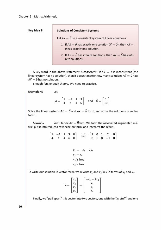
Chapter 2 Matrix Arithme c
..Key Idea 8
.
.Solu ons of Consistent Systems
Let Ax = b be a consistent system of linear equa ons.
1. If Ax = 0 has exactly one solu on (x = 0), then Ax =
b has exactly one solu on.
2. If Ax = 0 has infinite solu ons, then Ax = b has infi-nite solu ons.
A key word in the above statement is consistent. If Ax = b is inconsistent (thelinear system has no solu on), then it doesn’t ma er howmany solu ons Ax = 0 has;Ax = b has no solu on.
Enough fun, enough theory. We need to prac ce.
.. Example 47 ..Let
A =
[1 −1 1 34 2 4 6
]and b =
[110
].
Solve the linear systems Ax = 0 and Ax = b for x, and write the solu ons in vectorform.
S We’ll tackle Ax = 0 first. We form the associated augmented ma-trix, put it into reduced row echelon form, and interpret the result.[
1 −1 1 3 04 2 4 6 0
]−→rref
[1 0 1 2 00 1 0 −1 0
]
x1 = −x3 − 2x4x2 = x4x3 is free
x4 is free
To write our solu on in vector form, we rewrite x1 and x2 in x in terms of x3 and x4.
x =
x1x2x3x4
=
−x3 − 2x4
x4x3x4
Finally, we “pull apart” this vector into two vectors, onewith the “x3 stuff” and one
90
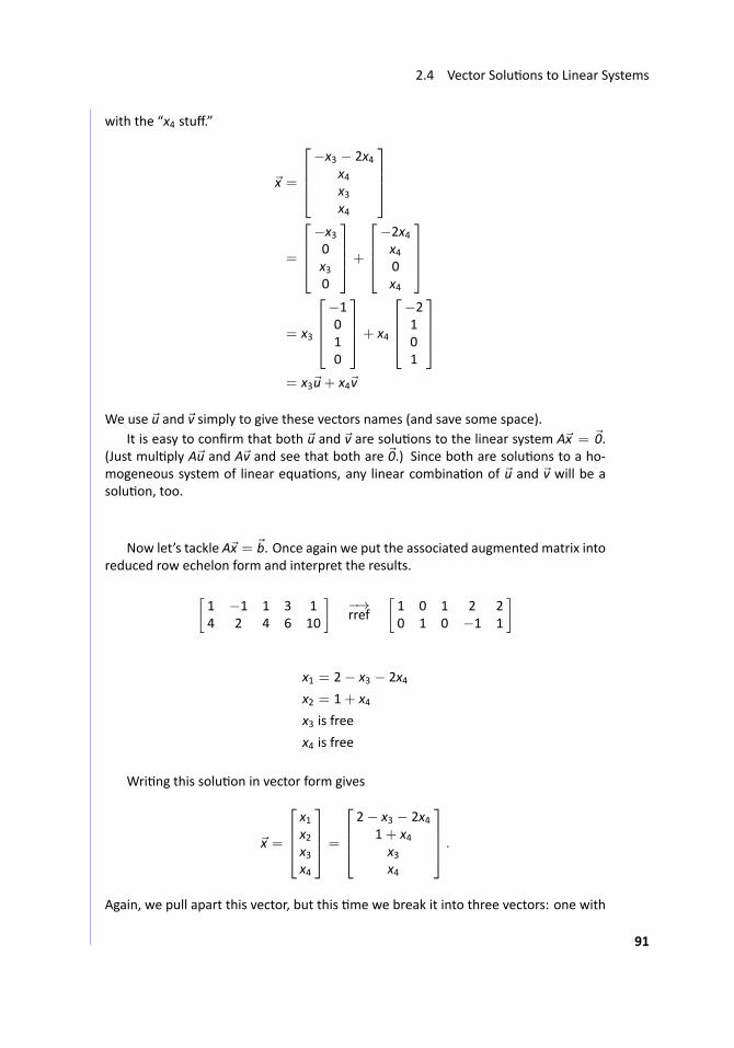
2.4 Vector Solu ons to Linear Systems
with the “x4 stuff.”
x =
−x3 − 2x4
x4x3x4
=
−x30x30
+
−2x4x40x4
= x3
−1010
+ x4
−2101
= x3u+ x4v
We use u and v simply to give these vectors names (and save some space).It is easy to confirm that both u and v are solu ons to the linear system Ax = 0.
(Just mul ply Au and Av and see that both are 0.) Since both are solu ons to a ho-mogeneous system of linear equa ons, any linear combina on of u and v will be asolu on, too.
..Now let’s tackle Ax = b. Once again we put the associated augmented matrix into
reduced row echelon form and interpret the results.
[1 −1 1 3 14 2 4 6 10
]−→rref
[1 0 1 2 20 1 0 −1 1
]
x1 = 2− x3 − 2x4x2 = 1+ x4x3 is free
x4 is free
Wri ng this solu on in vector form gives
x =
x1x2x3x4
=
2− x3 − 2x4
1+ x4x3x4
.
Again, we pull apart this vector, but this me we break it into three vectors: one with
91
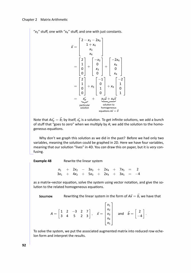
Chapter 2 Matrix Arithme c
“x3” stuff, one with “x4” stuff, and one with just constants.
x =
2− x3 − 2x4
1+ x4x3x4
=
2100
+
−x30x30
+
−2x4x40x4
=
2100
+ x3
−1010
+ x4
−2101
= xp︸︷︷︸
par cularsolu on
+ x3u+ x4v︸ ︷︷ ︸solu on to
homogeneousequa ons Ax = 0
Note that Axp = b; by itself, xp is a solu on. To get infinite solu ons, we add a bunchof stuff that “goes to zero” when we mul ply by A; we add the solu on to the homo-geneous equa ons.
Why don’t we graph this solu on as we did in the past? Before we had only twovariables, meaning the solu on could be graphed in 2D. Here we have four variables,meaning that our solu on “lives” in 4D. You can draw this on paper, but it is very con-fusing. ...
.. Example 48 ..Rewrite the linear system
x1 + 2x2 − 3x3 + 2x4 + 7x5 = 23x1 + 4x2 + 5x3 + 2x4 + 3x5 = −4
as a matrix–vector equa on, solve the system using vector nota on, and give the so-lu on to the related homogeneous equa ons.
S Rewri ng the linear system in the form of Ax = b, we have that
A =
[1 2 −3 2 73 4 5 2 3
], x =
x1x2x3x4x5
and b =
[2−4
].
To solve the system, we put the associated augmented matrix into reduced row eche-lon form and interpret the results.
92
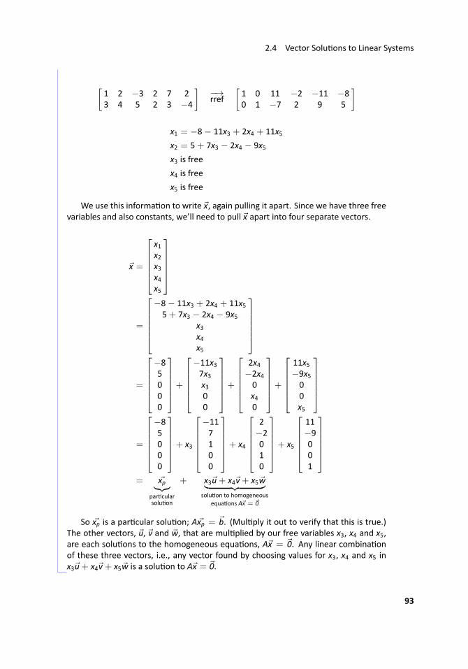
2.4 Vector Solu ons to Linear Systems
[1 2 −3 2 7 23 4 5 2 3 −4
]−→rref
[1 0 11 −2 −11 −80 1 −7 2 9 5
]
x1 = −8− 11x3 + 2x4 + 11x5x2 = 5+ 7x3 − 2x4 − 9x5x3 is free
x4 is free
x5 is free
We use this informa on to write x, again pulling it apart. Since we have three freevariables and also constants, we’ll need to pull x apart into four separate vectors.
x =
x1x2x3x4x5
=
−8− 11x3 + 2x4 + 11x55+ 7x3 − 2x4 − 9x5
x3x4x5
=
−85000
+
−11x37x3x300
+
2x4−2x40x40
+
11x5−9x500x5
=
−85000
+ x3
−117100
+ x4
2−2010
+ x5
11−9001
= xp︸︷︷︸
par cularsolu on
+ x3u+ x4v+ x5w︸ ︷︷ ︸solu on to homogeneous
equa ons Ax = 0
So xp is a par cular solu on; Axp = b. (Mul ply it out to verify that this is true.)The other vectors, u, v and w, that are mul plied by our free variables x3, x4 and x5,are each solu ons to the homogeneous equa ons, Ax = 0. Any linear combina onof these three vectors, i.e., any vector found by choosing values for x3, x4 and x5 inx3u+ x4v+ x5w is a solu on to Ax = 0. ...
93
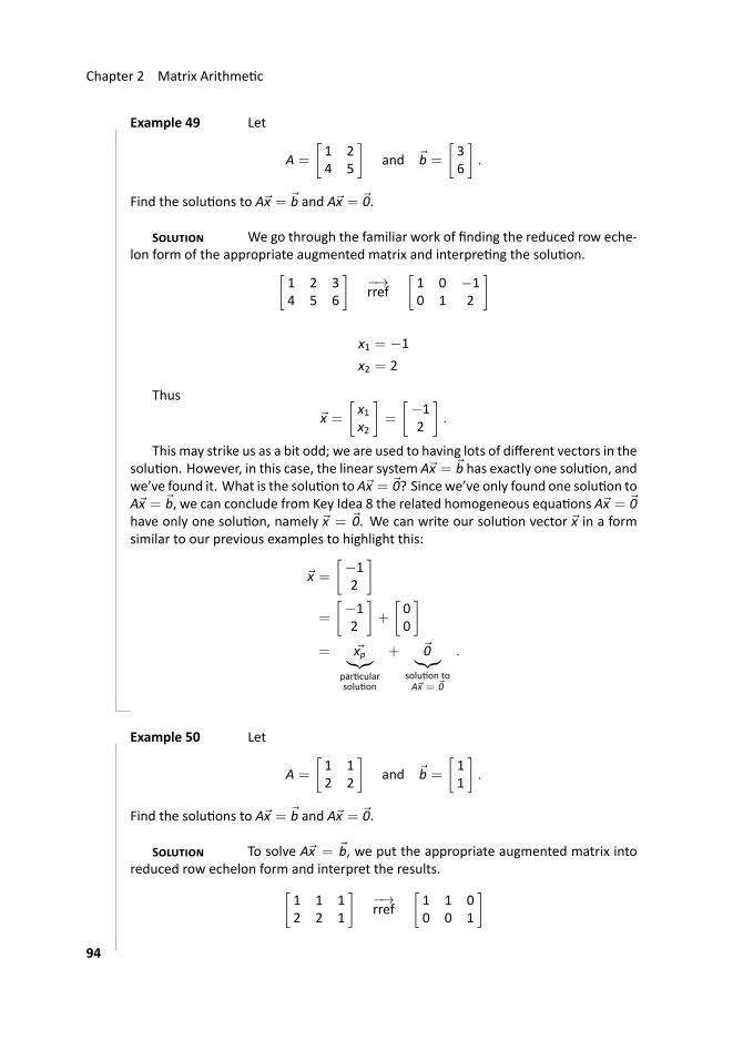
Chapter 2 Matrix Arithme c
.. Example 49 Let
A =
[1 24 5
]and b =
[36
].
Find the solu ons to Ax = b and Ax = 0.
S We go through the familiar work of finding the reduced row eche-lon form of the appropriate augmented matrix and interpre ng the solu on.[
1 2 34 5 6
]−→rref
[1 0 −10 1 2
]
x1 = −1
x2 = 2
Thus
x =
[x1x2
]=
[−12
].
This may strike us as a bit odd; we are used to having lots of different vectors in thesolu on. However, in this case, the linear system Ax = b has exactly one solu on, andwe’ve found it. What is the solu on to Ax = 0? Since we’ve only found one solu on toAx = b, we can conclude from Key Idea 8 the related homogeneous equa ons Ax = 0have only one solu on, namely x = 0. We can write our solu on vector x in a formsimilar to our previous examples to highlight this:
x =
[−12
]=
[−12
]+
[00
]= xp︸︷︷︸
par cularsolu on
+ 0︸︷︷︸solu on toAx = 0
.
..
.. Example 50 ..Let
A =
[1 12 2
]and b =
[11
].
Find the solu ons to Ax = b and Ax = 0.
S To solve Ax = b, we put the appropriate augmented matrix intoreduced row echelon form and interpret the results.[
1 1 12 2 1
]−→rref
[1 1 00 0 1
]94
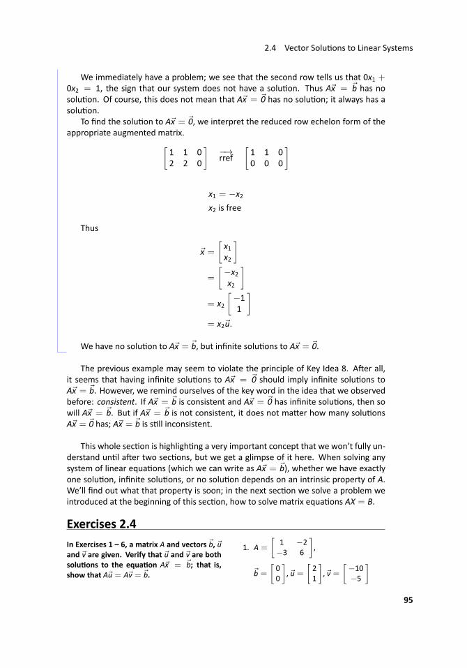
2.4 Vector Solu ons to Linear Systems
We immediately have a problem; we see that the second row tells us that 0x1 +0x2 = 1, the sign that our system does not have a solu on. Thus Ax = b has nosolu on. Of course, this does not mean that Ax = 0 has no solu on; it always has asolu on.
To find the solu on to Ax = 0, we interpret the reduced row echelon form of theappropriate augmented matrix.[
1 1 02 2 0
]−→rref
[1 1 00 0 0
]
x1 = −x2x2 is free
Thus
x =
[x1x2
]=
[−x2x2
]= x2
[−11
]= x2u.
We have no solu on to Ax = b, but infinite solu ons to Ax = 0. ...
The previous example may seem to violate the principle of Key Idea 8. A er all,it seems that having infinite solu ons to Ax = 0 should imply infinite solu ons toAx = b. However, we remind ourselves of the key word in the idea that we observedbefore: consistent. If Ax = b is consistent and Ax = 0 has infinite solu ons, then sowill Ax = b. But if Ax = b is not consistent, it does not ma er how many solu onsAx = 0 has; Ax = b is s ll inconsistent.
This whole sec on is highligh ng a very important concept that we won’t fully un-derstand un l a er two sec ons, but we get a glimpse of it here. When solving anysystem of linear equa ons (which we can write as Ax = b), whether we have exactlyone solu on, infinite solu ons, or no solu on depends on an intrinsic property of A.We’ll find out what that property is soon; in the next sec on we solve a problem weintroduced at the beginning of this sec on, how to solve matrix equa ons AX = B.
Exercises 2.4In Exercises 1 – 6, a matrix A and vectors b, uand v are given. Verify that u and v are bothsolu ons to the equa on Ax = b; that is,show that Au = Av = b.
1. A =
[1 −2−3 6
],
b =
[00
], u =
[21
], v =
[−10−5
]95
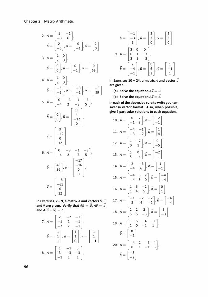
Chapter 2 Matrix Arithme c
2. A =
[1 −2−3 6
],
b =
[2−6
], u =
[0−1
], v =
[20
]3. A =
[1 02 0
],
b =
[00
], u =
[0−1
], v =
[059
]4. A =
[1 02 0
],
b =
[−3−6
], u =
[−3−1
], v =
[−359
]5. A =
[0 −3 −1 −3−4 2 −3 5
],
b =
[00
], u =
114
−120
,
v =
9
−12012
6. A =
[0 −3 −1 −3−4 2 −3 5
],
b =
[4836
], u =
−17−1600
,
v =
−8−28012
In Exercises 7 – 9, a matrix A and vectors b, uand v are given. Verify that Au = 0, Av = band A(u+ v) = b.
7. A =
2 −2 −1−1 1 −1−2 2 −1
,b =
111
, u =
110
, v = 1
1−1
8. A =
1 −1 33 −3 −3−1 1 1
,
b =
−1−31
, u =
220
, v = 230
9. A =
2 0 00 1 −33 1 −3
,b =
2−4−1
, u =
062
, v = 1−11
In Exercises 10 – 24, a matrix A and vector bare given.
(a) Solve the equa on Ax = 0.
(b) Solve the equa on Ax = b.
In each of the above, be sure towrite your an-swer in vector format. Also, when possible,give 2 par cular solu ons to each equa on.
10. A =
[0 2−1 3
], b =
[−2−1
]11. A =
[−4 −1−3 −2
], b =
[14
]12. A =
[1 −20 1
], b =
[0−5
]13. A =
[1 05 −4
], b =
[−2−1
]14. A =
[2 −3−4 6
], b =
[1−1
]15. A =
[−4 3 2−4 5 0
], b =
[−4−4
]16. A =
[1 5 −21 4 5
], b =
[01
]17. A =
[−1 −2 −23 4 −2
], b =
[−4−4
]18. A =
[2 2 25 5 −3
], b =
[3−3
]19. A =
[1 5 −4 −11 0 −2 1
],
b =
[0−2
]20. A =
[−4 2 −5 40 1 −1 5
],
b =
[−3−2
]96
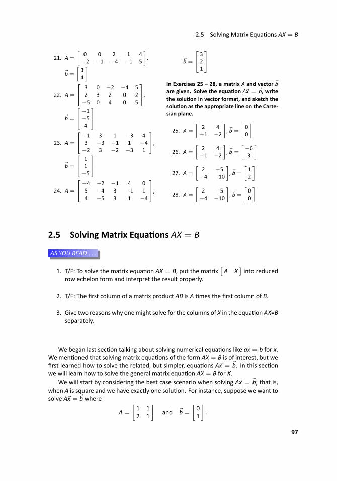
2.5 Solving Matrix Equa ons AX = B
21. A =
[0 0 2 1 4−2 −1 −4 −1 5
],
b =
[34
]
22. A =
3 0 −2 −4 52 3 2 0 2−5 0 4 0 5
,b =
−1−54
23. A =
−1 3 1 −3 43 −3 −1 1 −4−2 3 −2 −3 1
,b =
11−5
24. A =
−4 −2 −1 4 05 −4 3 −1 14 −5 3 1 −4
,
b =
321
In Exercises 25 – 28, a matrix A and vector bare given. Solve the equa on Ax = b, writethe solu on in vector format, and sketch thesolu on as the appropriate line on the Carte-sian plane.
25. A =
[2 4−1 −2
], b =
[00
]
26. A =
[2 4−1 −2
], b =
[−63
]
27. A =
[2 −5−4 −10
], b =
[12
]
28. A =
[2 −5−4 −10
], b =
[00
]
2.5 Solving Matrix Equa ons AX = B
...AS YOU READ . . .
1. T/F: To solve the matrix equa on AX = B, put the matrix[A X
]into reduced
row echelon form and interpret the result properly.
2. T/F: The first column of a matrix product AB is A mes the first column of B.
3. Give two reasons why onemight solve for the columns of X in the equa on AX=Bseparately.
We began last sec on talking about solving numerical equa ons like ax = b for x.We men oned that solving matrix equa ons of the form AX = B is of interest, but wefirst learned how to solve the related, but simpler, equa ons Ax = b. In this sec onwe will learn how to solve the general matrix equa on AX = B for X.
We will start by considering the best case scenario when solving Ax = b; that is,when A is square and we have exactly one solu on. For instance, suppose we want tosolve Ax = b where
A =
[1 12 1
]and b =
[01
].
97
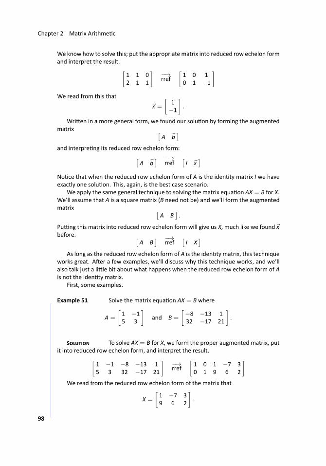
Chapter 2 Matrix Arithme c
We know how to solve this; put the appropriate matrix into reduced row echelon formand interpret the result. [
1 1 02 1 1
]−→rref
[1 0 10 1 −1
]We read from this that
x =
[1−1
].
Wri en in a more general form, we found our solu on by forming the augmentedmatrix [
A b]
and interpre ng its reduced row echelon form:[A b
] −→rref
[I x
]No ce that when the reduced row echelon form of A is the iden ty matrix I we haveexactly one solu on. This, again, is the best case scenario.
We apply the same general technique to solving the matrix equa on AX = B for X.We’ll assume that A is a square matrix (B need not be) and we’ll form the augmentedmatrix [
A B].
Pu ng this matrix into reduced row echelon form will give us X, much like we found xbefore. [
A B] −→
rref[I X
]As long as the reduced row echelon form of A is the iden ty matrix, this technique
works great. A er a few examples, we’ll discuss why this technique works, and we’llalso talk just a li le bit about what happens when the reduced row echelon form of Ais not the iden ty matrix.
First, some examples.
.. Example 51 ..Solve the matrix equa on AX = B where
A =
[1 −15 3
]and B =
[−8 −13 132 −17 21
].
S To solve AX = B for X, we form the proper augmented matrix, putit into reduced row echelon form, and interpret the result.[
1 −1 −8 −13 15 3 32 −17 21
]−→rref
[1 0 1 −7 30 1 9 6 2
]We read from the reduced row echelon form of the matrix that
X =
[1 −7 39 6 2
].
98
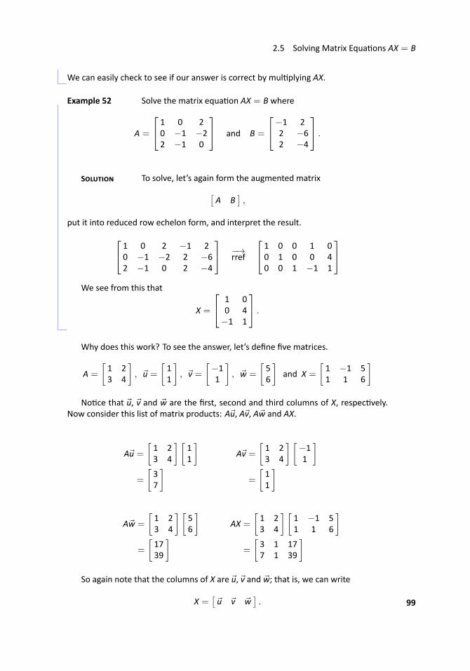
2.5 Solving Matrix Equa ons AX = B
We can easily check to see if our answer is correct by mul plying AX. ...
.. Example 52 Solve the matrix equa on AX = B where
A =
1 0 20 −1 −22 −1 0
and B =
−1 22 −62 −4
.
S To solve, let’s again form the augmented matrix[A B
],
put it into reduced row echelon form, and interpret the result. 1 0 2 −1 20 −1 −2 2 −62 −1 0 2 −4
−→rref
1 0 0 1 00 1 0 0 40 0 1 −1 1
We see from this that
X =
1 00 4−1 1
.
..
Why does this work? To see the answer, let’s define five matrices.
A =
[1 23 4
], u =
[11
], v =
[−11
], w =
[56
]and X =
[1 −1 51 1 6
]No ce that u, v and w are the first, second and third columns of X, respec vely.
Now consider this list of matrix products: Au, Av, Aw and AX.
Au =
[1 23 4
] [11
]=
[37
]
Aw =
[1 23 4
] [56
]=
[1739
]
Av =[1 23 4
] [−11
]=
[11
]
AX =
[1 23 4
] [1 −1 51 1 6
]=
[3 1 177 1 39
]So again note that the columns of X are u, v and w; that is, we can write
X =[u v w
]. 99
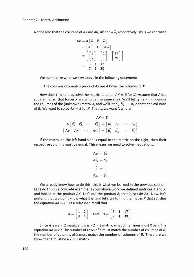
Chapter 2 Matrix Arithme c
No ce also that the columns of AX are Au, Av and Aw, respec vely. Thus we can write
AX = A[u v w
]=
[Au Av Aw
]=
[ [37
] [11
] [1739
] ]=
[3 1 177 1 39
]We summarize what we saw above in the following statement:
The columns of a matrix product AX are A mes the columns of X.
How does this help us solve the matrix equa on AX = B for X? Assume that A is asquare matrix (that forces X and B to be the same size). We’ll let x1, x2, · · · xn denotethe columns of the (unknown) matrix X, and we’ll let b1, b2, · · · bn denote the columnsof B. We want to solve AX = B for X. That is, we want X where
AX = B
A[x1 x2 · · · xn
]=
[b1 b2 · · · bn
][Ax1 Ax2 · · · Axn
]=
[b1 b2 · · · bn
]If the matrix on the le hand side is equal to the matrix on the right, then their
respec ve columns must be equal. This means we need to solve n equa ons:
Ax1 = b1
Ax2 = b2... =
...
Axn = bn
We already know how to do this; this is what we learned in the previous sec on.Let’s do this in a concrete example. In our above work we defined matrices A and X,and looked at the product AX. Let’s call the product B; that is, set B= AX. Now, let’spretend that we don’t know what X is, and let’s try to find the matrix X that sa sfiesthe equa on AX = B. As a refresher, recall that
A =
[1 23 4
]and B =
[3 1 177 1 39
].
Since A is a 2× 2 matrix and B is a 2× 3 matrix, what dimensions must X be in theequa on AX = B? The number of rows of Xmust match the number of columns of A;the number of columns of X must match the number of columns of B. Therefore weknow that Xmust be a 2× 3 matrix.
100
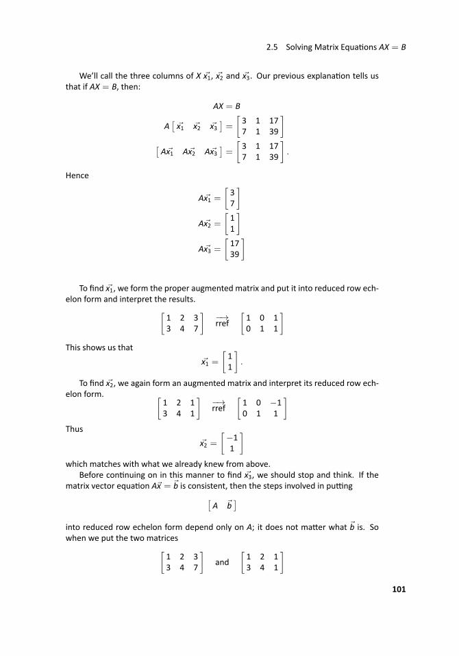
2.5 Solving Matrix Equa ons AX = B
We’ll call the three columns of X x1, x2 and x3. Our previous explana on tells usthat if AX = B, then:
AX = B
A[x1 x2 x3
]=
[3 1 177 1 39
][Ax1 Ax2 Ax3
]=
[3 1 177 1 39
].
Hence
Ax1 =[37
]Ax2 =
[11
]Ax3 =
[1739
]
To find x1, we form the proper augmented matrix and put it into reduced row ech-elon form and interpret the results.[
1 2 33 4 7
]−→rref
[1 0 10 1 1
]This shows us that
x1 =[11
].
To find x2, we again form an augmented matrix and interpret its reduced row ech-elon form. [
1 2 13 4 1
]−→rref
[1 0 −10 1 1
]Thus
x2 =[−11
]which matches with what we already knew from above.
Before con nuing on in this manner to find x3, we should stop and think. If thematrix vector equa on Ax = b is consistent, then the steps involved in pu ng[
A b]
into reduced row echelon form depend only on A; it does not ma er what b is. Sowhen we put the two matrices[
1 2 33 4 7
]and
[1 2 13 4 1
]101
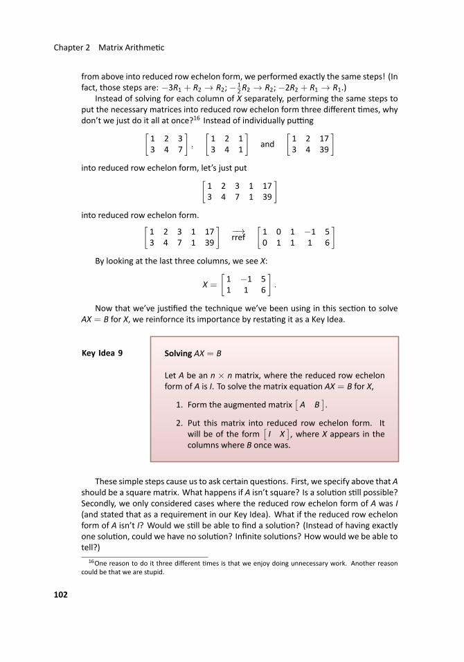
Chapter 2 Matrix Arithme c
from above into reduced row echelon form, we performed exactly the same steps! (Infact, those steps are: −3R1 + R2 → R2;− 1
2R2 → R2;−2R2 + R1 → R1.)Instead of solving for each column of X separately, performing the same steps to
put the necessary matrices into reduced row echelon form three different mes, whydon’t we just do it all at once?16 Instead of individually pu ng[
1 2 33 4 7
],
[1 2 13 4 1
]and
[1 2 173 4 39
]into reduced row echelon form, let’s just put[
1 2 3 1 173 4 7 1 39
]into reduced row echelon form.[
1 2 3 1 173 4 7 1 39
]−→rref
[1 0 1 −1 50 1 1 1 6
]By looking at the last three columns, we see X:
X =
[1 −1 51 1 6
].
Now that we’ve jus fied the technique we’ve been using in this sec on to solveAX = B for X, we reinfornce its importance by resta ng it as a Key Idea.
..Key Idea 9
.
.Solving AX = B
Let A be an n × n matrix, where the reduced row echelonform of A is I. To solve the matrix equa on AX = B for X,
1. Form the augmented matrix[A B
].
2. Put this matrix into reduced row echelon form. Itwill be of the form
[I X
], where X appears in the
columns where B once was.
These simple steps cause us to ask certain ques ons. First, we specify above that Ashould be a square matrix. What happens if A isn’t square? Is a solu on s ll possible?Secondly, we only considered cases where the reduced row echelon form of A was I(and stated that as a requirement in our Key Idea). What if the reduced row echelonform of A isn’t I? Would we s ll be able to find a solu on? (Instead of having exactlyone solu on, could we have no solu on? Infinite solu ons? How would we be able totell?)
16One reason to do it three different mes is that we enjoy doing unnecessary work. Another reasoncould be that we are stupid.
102
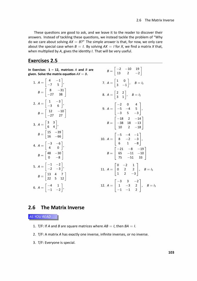
2.6 The Matrix Inverse
These ques ons are good to ask, and we leave it to the reader to discover theiranswers. Instead of tackling these ques ons, we instead tackle the problem of “Whydo we care about solving AX = B?” The simple answer is that, for now, we only careabout the special case when B = I. By solving AX = I for X, we find a matrix X that,when mul plied by A, gives the iden ty I. That will be very useful.
Exercises 2.5
In Exercises 1 – 12, matrices A and B aregiven. Solve the matrix equa on AX = B.
1. A =
[4 −1−7 5
],
B =
[8 −31
−27 38
]2. A =
[1 −3−3 6
],
B =
[12 −10−27 27
]3. A =
[3 36 4
],
B =
[15 −3916 −66
]4. A =
[−3 −64 0
],
B =
[48 −300 −8
]5. A =
[−1 −2−2 −3
],
B =
[13 4 722 5 12
]6. A =
[−4 1−1 −2
],
B =
[−2 −10 1913 2 −2
]
7. A =
[1 03 −1
], B = I2
8. A =
[2 23 1
], B = I2
9. A =
−2 0 4−5 −4 5−3 5 −3
,B =
−18 2 −14−38 18 −1310 2 −18
10. A =
−5 −4 −18 −2 −36 1 −8
,B =
−21 −8 −1965 −11 −1075 −51 33
11. A =
0 −2 10 2 21 2 −3
, B = I3
12. A =
−3 3 −21 −3 2−1 −1 2
, B = I3
2.6 The Matrix Inverse...AS YOU READ . . .
1. T/F: If A and B are square matrices where AB = I, then BA = I.
2. T/F: A matrix A has exactly one inverse, infinite inverses, or no inverse.
3. T/F: Everyone is special.
103
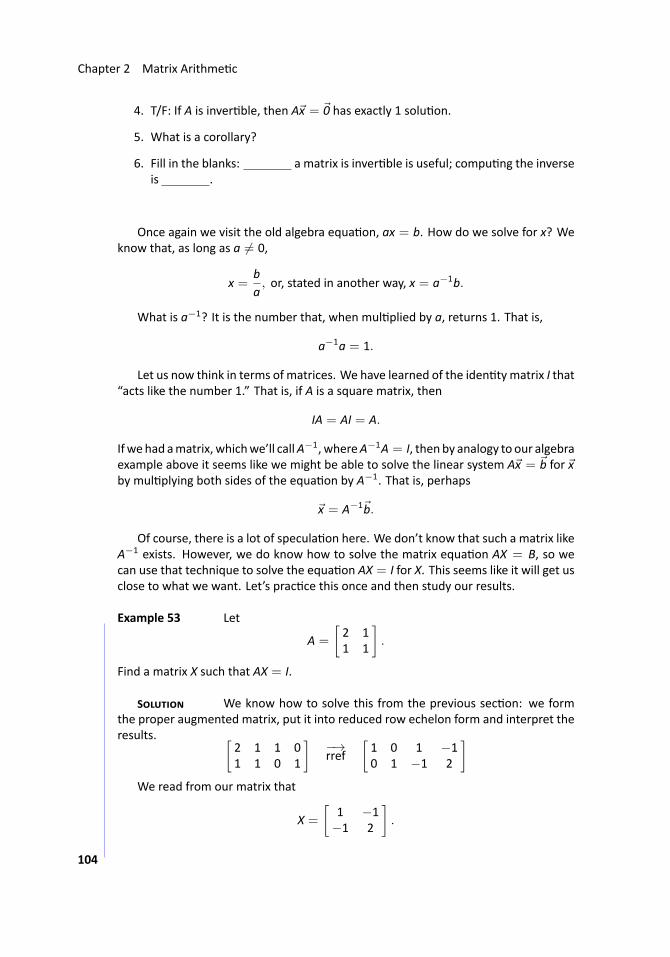
Chapter 2 Matrix Arithme c
4. T/F: If A is inver ble, then Ax = 0 has exactly 1 solu on.
5. What is a corollary?
6. Fill in the blanks: a matrix is inver ble is useful; compu ng the inverseis .
Once again we visit the old algebra equa on, ax = b. How do we solve for x? Weknow that, as long as a = 0,
x =ba, or, stated in another way, x = a−1b.
What is a−1? It is the number that, when mul plied by a, returns 1. That is,
a−1a = 1.
Let us now think in terms of matrices. We have learned of the iden ty matrix I that“acts like the number 1.” That is, if A is a square matrix, then
IA = AI = A.
If wehad amatrix, whichwe’ll callA−1, whereA−1A = I, thenby analogy to our algebraexample above it seems like we might be able to solve the linear system Ax = b for xby mul plying both sides of the equa on by A−1. That is, perhaps
x = A−1b.
Of course, there is a lot of specula on here. We don’t know that such a matrix likeA−1 exists. However, we do know how to solve the matrix equa on AX = B, so wecan use that technique to solve the equa on AX = I for X. This seems like it will get usclose to what we want. Let’s prac ce this once and then study our results.
.. Example 53 ..Let
A =
[2 11 1
].
Find a matrix X such that AX = I.
S We know how to solve this from the previous sec on: we formthe proper augmented matrix, put it into reduced row echelon form and interpret theresults. [
2 1 1 01 1 0 1
]−→rref
[1 0 1 −10 1 −1 2
]We read from our matrix that
X =
[1 −1−1 2
].
104
2.6 The Matrix Inverse
Let’s check our work:
AX =
[2 11 1
] [1 −1−1 2
]=
[1 00 1
]= I
Sure enough, it works. ...
Looking at our previous example, we are tempted to jump in and call the matrix Xthat we found “A−1.” However, there are two obstacles in the way of us doing this.
First, we know that in general AB = BA. So while we found that AX = I, we can’tautoma cally assume that XA = I.
Secondly, we have seen examples of matrices where AB = AC, but B = C. So justbecause AX = I, it is possible that another matrix Y exists where AY = I. If this is thecase, using the nota on A−1 would be misleading, since it could refer to more thanone matrix.
These obstacles that we face are not insurmountable. The first obstacle was thatwe know that AX = I but didn’t know that XA = I. That’s easy enough to check,though. Let’s look at A and X from our previous example.
XA =
[1 −1−1 2
] [2 11 1
]=
[1 00 1
]= I
Perhaps this first obstacle isn’t much of an obstacle a er all. Of course, we onlyhave one example where it worked, so this doesn’t mean that it always works. Wehave good news, though: it always does work. The only “bad” news to come with thisis that this is a bit harder to prove. We won’t worry about proving it always works, butstate formally that it does in the following theorem.
..Theorem 5
.
.Special Commu ng Matrix Products
Let A be an n× nmatrix.
1. If there is a matrix X such that AX = In, then XA = In.
2. If there is a matrix X such that XA = In, then AX = In.
The second obstacle is easier to address. We want to know if another matrix Yexists where AY = I = YA. Let’s suppose that it does. Consider the expression XAY.
105
Chapter 2 Matrix Arithme c
Since matrix mul plica on is associa ve, we can group this any way we choose. Wecould group this as (XA)Y; this results in
(XA)Y = IY
= Y.
We could also group XAY as X(AY). This tells us
X(AY) = XI
= X
Combining the two ideas above, we see that X = XAY = Y; that is, X = Y. Weconclude that there is only one matrix X where XA = I = AX. (Even if we think wehave two, we can do the above exercise and see that we really just have one.)
We have just proved the following theorem.
..Theorem 6
.
.Uniqueness of Solu ons to AX = In
Let A be an n × n matrix and let X be a matrix where AX =In. Then X is unique; it is the only matrix that sa sfies thisequa on.
So given a square matrix A, if we can find a matrix X where AX = I, then we knowthat XA = I and that X is the only matrix that does this. This makes X special, so wegive it a special name.
..Defini on 18
.
.Inver ble Matrices and the Inverse of A
Let A and X be n× nmatrices where AX = I = XA. Then:
1. A is inver ble.
2. X is the inverse of A, denoted by A−1.
Let’s do an example.
.. Example 54 ..Find the inverse of A =
[1 22 4
].
S By solving the equa on AX = I for X will give us the inverse of A.Forming the appropriate augmented matrix and finding its reduced row echelon form
106
2.6 The Matrix Inverse
gives us [1 2 1 02 4 0 1
]−→rref
[1 2 0 1/20 0 1 −1/2
]Yikes! We were expec ng to find that the reduced row echelon form of this matrixwould look like [
I A−1].
However, we don’t have the iden ty on the le hand side. Our conclusion: A is notinver ble. ...
We have just seen that not all matrices are inver ble.17 With this thought in mind,let’s complete the array of boxes we started before the example. We’ve discoveredthat if a matrix has an inverse, it has only one. Therefore, we gave that special matrixa name, “the inverse.” Finally, we describe the most general way to find the inverse ofa matrix, and a way to tell if it does not have one.
..Key Idea 10
.
.Finding A−1
Let A be an n × n matrix. To find A−1, put the augmentedmatrix [
A In]
into reduced row echelon form. If the result is of the form[In X
],
then A−1 = X. If not, (that is, if the first n columns of the re-duced row echelon form are not In), then A is not inver ble.
Let’s try again.
.. Example 55 ..Find the inverse, if it exists, of A =
1 1 −11 −1 11 2 3
.S We’ll try to solve AX = I for X and see what happens. 1 1 −1 1 0 0
1 −1 1 0 1 01 2 3 0 0 1
−→rref
1 0 0 0.5 0.5 00 1 0 0.2 −0.4 0.20 0 1 −0.3 0.1 0.2
17Hence our previous defini on; why bother calling A “inver ble” if every square matrix is? If everyone
is special, then no one is. Then again, everyone is special.
107
Chapter 2 Matrix Arithme c
We have a solu on, so
A =
0.5 0.5 00.2 −0.4 0.2−0.3 0.1 0.2
.
Mul ply AA−1 to verify that it is indeed the inverse of A. ...
In general, given a matrix A, to find A−1 we need to form the augmented matrix[A I
]and put it into reduced row echelon form and interpret the result. In the case
of a 2 × 2 matrix, though, there is a shortcut. We give the shortcut in terms of atheorem.18
..Theorem 7
.
.The Inverse of a 2×2 Matrix
Let
A =
[a bc d
].
A is inver ble if and only if ad− bc = 0.
If ad− bc = 0, then
A−1 =1
ad− bc
[d −b−c a
].
We can’t divide by 0, so if ad− bc = 0, we don’t have an inverse. Recall Example54, where
A =
[1 22 4
].
Here, ad− bc = 1(4)− 2(2) = 0, which is why A didn’t have an inverse.Although this idea is simple, we should prac ce it.
.. Example 56 ..Use Theorem 7 to find the inverse of
A =
[3 2−1 9
]if it exists.
18We don’t prove this theorem here, but it really isn’t hard to do. Put the matrix[a b 1 0c d 0 1
]into reduced row echelon form and you’ll discover the result of the theorem. Alterna vely, mul ply A bywhat we propose is the inverse and see that we indeed get I.108
2.6 The Matrix Inverse
S Since ad− bc = 29 = 0, A−1 exists. By the Theorem,
A−1 =1
3(9)− 2(−1)
[9 −21 3
]=
129
[9 −21 3
]
We can leave our answer in this form, or we could “simplify” it as
A−1 =129
[9 −21 3
]=
[9/29 −2/291/29 3/29
].
...
We started this sec on out by specula ng that just as we solved algebraic equa-ons of the form ax = b by compu ng x = a−1b, we might be able to solve matrix
equa ons of the form Ax = b by compu ng x = A−1b. If A−1 does exist, then we cansolve the equa on Ax = b this way. Consider:
Ax = b (original equa on)
A−1Ax = A−1b (mul ply both sides on the le by A−1)
Ix = A−1b (since A−1A = I)
x = A−1b (since Ix = x)
Let’s step back and think about this for a moment. The only thing we know aboutthe equa on Ax = b is that A is inver ble. We also know that solu ons to Ax = bcome in three forms: exactly one solu on, infinite solu ons, and no solu on. We justshowed that if A is inver ble, then Ax = b has at least one solu on. We showed thatby se ng x equal to A−1b, we have a solu on. Is it possible that more solu ons exist?
No. Supposewe are told that a known vector v is a solu on to the equa onAx = b;that is, we know that Av = b. We can repeat the above steps:
Av = b
A−1Av = A−1b
Iv = A−1b
v = A−1b.
This shows that all solu ons to Ax = b are exactly x = A−1b when A is inver ble. Wehave just proved the following theorem.
109
Chapter 2 Matrix Arithme c
..Theorem 8
.
.Inver ble Matrices and Solu ons to Ax = b
Let A be an inver ble n × n matrix, and let b be any n × 1column vector. Then the equa on Ax = b has exactly onesolu on, namely
x = A−1b.
A corollary19 to this theorem is: If A is not inver ble, then Ax = b does not haveexactly one solu on. It may have infinite solu ons and it may have no solu on, andwe would need to examine the reduced row echelon form of the augmented matrix[A b
]to see which case applies.
We demonstrate our theorem with an example.
.. Example 57 Solve Ax = b by compu ng x = A−1b, where
A =
1 0 −3−3 −4 104 −5 −11
and b =
−1557−46
.
S Without showing our steps, we compute
A−1 =
94 15 −127 1 −131 5 −4
.
We then find the solu on to Ax = b by compu ng A−1b:
x = A−1b
=
94 15 −127 1 −131 5 −4
−1557−46
=
−3−24
.
We can easily check our answer: 1 0 −3−3 −4 104 −5 −11
−3−24
=
−1557−46
.
..
19a corollary is an idea that follows directly from a theorem
110
2.6 The Matrix Inverse
Knowing a matrix is inver ble is incredibly useful.20 Among many other reasons, ifyou know A is inver ble, then you know for sure that Ax = b has a solu on (as we juststated in Theorem 8). In the next sec on we’ll demonstrate many different proper esof inver ble matrices, including sta ng several different ways in which we know thata matrix is inver ble.
Exercises 2.6In Exercises 1 – 8, A matrix A is given. FindA−1 using Theorem 7, if it exists.
1.[
1 5−5 −24
]2.
[1 −41 −3
]3.
[3 00 7
]4.
[2 53 4
]5.
[1 −3−2 6
]6.
[3 72 4
]7.
[1 00 1
]8.
[0 11 0
]In Exercises 9 – 28, a matrix A is given. FindA−1 using Key Idea 10, if it exists.
9.[−2 31 5
]10.
[−5 −29 2
]11.
[1 23 4
]12.
[5 7
5/3 7/3
]
13.
25 −10 −4−18 7 3−6 2 1
14.
2 3 4−3 6 9−1 9 13
15.
1 0 04 1 −720 7 −48
16.
−4 1 5−5 1 9−10 2 19
17.
5 −1 07 7 1−2 −8 −1
18.
1 −5 0−2 15 44 −19 1
19.
25 −8 0−78 25 048 −15 1
20.
1 0 07 5 8−2 −2 −3
21.
0 0 11 0 00 1 0
22.
0 1 01 0 00 0 1
23.
1 0 0 0
−19 −9 0 433 4 1 −74 2 0 −1
24.
1 0 0 027 1 0 418 0 1 44 0 0 1
20As odd as it may sound, knowing a matrix is inver ble is useful; actually compu ng the inverse isn’t.
This is discussed at the end of the next sec on.
111
Chapter 2 Matrix Arithme c
25.
−15 45 −3 455 −164 15 −15
−215 640 −62 59−4 12 0 1
26.
1 0 2 80 1 0 00 −4 −29 −1100 −3 −5 −19
27.
0 0 1 00 0 0 11 0 0 00 1 0 0
28.
1 0 0 00 2 0 00 0 3 00 0 0 −4
In Exercises 29 – 36, a matrix A and a vectorb are given. Solve the equa on Ax = b usingTheorem 8.
29. A =
[3 52 3
], b =
[2113
]
30. A =
[1 −44 −15
], b =
[2177
]
31. A =
[9 70−4 −31
], b =
[−21
]
32. A =
[10 −573 −17
], b =
[−14−4
]
33. A =
1 2 120 1 6−3 0 1
,
b =
−17−520
34. A =
1 0 −38 −2 −1312 −3 −20
,
b =
−34−159−243
35. A =
5 0 −2−8 1 5−2 0 1
,
b =
33−70−15
36. A =
1 −6 00 1 02 −8 1
,
b =
−6910
−102
2.7 Proper es of the Matrix Inverse
...AS YOU READ . . .
1. What does it mean to say that two statements are “equivalent?”
2. T/F: If A is not inver ble, then Ax = 0 could have no solu ons.
3. T/F: If A is not inver ble, then Ax = b could have infinite solu ons.
4. What is the inverse of the inverse of A?
5. T/F: Solving Ax = b using Gaussian elimina on is faster than using the inverseof A.
We ended the previous sec on by sta ng that inver ble matrices are important.Since they are, in this sec on we study inver ble matrices in two ways. First, we look
112
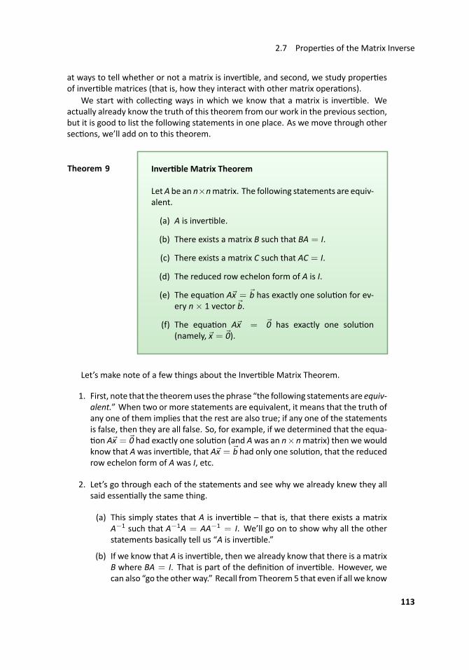
2.7 Proper es of the Matrix Inverse
at ways to tell whether or not a matrix is inver ble, and second, we study proper esof inver ble matrices (that is, how they interact with other matrix opera ons).
We start with collec ng ways in which we know that a matrix is inver ble. Weactually already know the truth of this theorem from our work in the previous sec on,but it is good to list the following statements in one place. As we move through othersec ons, we’ll add on to this theorem.
..Theorem 9
.
.Inver ble Matrix Theorem
LetA be an n×nmatrix. The following statements are equiv-alent.
(a) A is inver ble.
(b) There exists a matrix B such that BA = I.
(c) There exists a matrix C such that AC = I.
(d) The reduced row echelon form of A is I.
(e) The equa on Ax = b has exactly one solu on for ev-ery n× 1 vector b.
(f) The equa on Ax = 0 has exactly one solu on(namely, x = 0).
Let’s make note of a few things about the Inver ble Matrix Theorem.
1. First, note that the theoremuses the phrase “the following statements are equiv-alent.” When two or more statements are equivalent, it means that the truth ofany one of them implies that the rest are also true; if any one of the statementsis false, then they are all false. So, for example, if we determined that the equa-on Ax = 0 had exactly one solu on (and Awas an n×nmatrix) then we would
know that Awas inver ble, that Ax = b had only one solu on, that the reducedrow echelon form of A was I, etc.
2. Let’s go through each of the statements and see why we already knew they allsaid essen ally the same thing.
(a) This simply states that A is inver ble – that is, that there exists a matrixA−1 such that A−1A = AA−1 = I. We’ll go on to show why all the otherstatements basically tell us “A is inver ble.”
(b) If we know that A is inver ble, then we already know that there is a matrixB where BA = I. That is part of the defini on of inver ble. However, wecan also “go the otherway.” Recall from Theorem5 that even if all we know
113
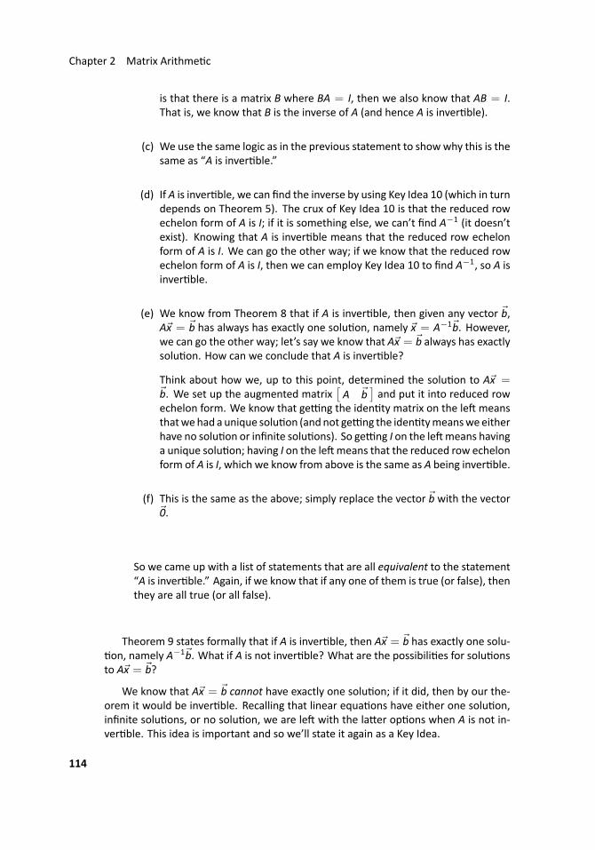
Chapter 2 Matrix Arithme c
is that there is a matrix B where BA = I, then we also know that AB = I.That is, we know that B is the inverse of A (and hence A is inver ble).
(c) We use the same logic as in the previous statement to showwhy this is thesame as “A is inver ble.”
(d) If A is inver ble, we can find the inverse by using Key Idea 10 (which in turndepends on Theorem 5). The crux of Key Idea 10 is that the reduced rowechelon form of A is I; if it is something else, we can’t find A−1 (it doesn’texist). Knowing that A is inver ble means that the reduced row echelonform of A is I. We can go the other way; if we know that the reduced rowechelon form of A is I, then we can employ Key Idea 10 to find A−1, so A isinver ble.
(e) We know from Theorem 8 that if A is inver ble, then given any vector b,Ax = b has always has exactly one solu on, namely x = A−1b. However,we can go the other way; let’s say we know that Ax = b always has exactlysolu on. How can we conclude that A is inver ble?
Think about how we, up to this point, determined the solu on to Ax =b. We set up the augmented matrix
[A b
]and put it into reduced row
echelon form. We know that ge ng the iden ty matrix on the le meansthatwehad aunique solu on (andnot ge ng the iden tymeansweeitherhave no solu on or infinite solu ons). So ge ng I on the le means havinga unique solu on; having I on the le means that the reduced row echelonform of A is I, which we know from above is the same as A being inver ble.
(f) This is the same as the above; simply replace the vector b with the vector0.
So we came up with a list of statements that are all equivalent to the statement“A is inver ble.” Again, if we know that if any one of them is true (or false), thenthey are all true (or all false).
Theorem 9 states formally that if A is inver ble, then Ax = b has exactly one solu-on, namely A−1b. What if A is not inver ble? What are the possibili es for solu ons
to Ax = b?
We know that Ax = b cannot have exactly one solu on; if it did, then by our the-orem it would be inver ble. Recalling that linear equa ons have either one solu on,infinite solu ons, or no solu on, we are le with the la er op ons when A is not in-ver ble. This idea is important and so we’ll state it again as a Key Idea.
114
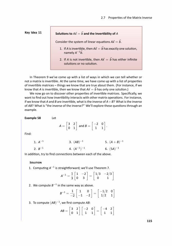
2.7 Proper es of the Matrix Inverse
..Key Idea 11
.
.Solu ons to Ax = b and the Inver bility of A
Consider the system of linear equa ons Ax = b.
1. IfA is inver ble, then Ax = b has exactly one solu on,namely A−1b.
2. If A is not inver ble, then Ax = b has either infinitesolu ons or no solu on.
In Theorem 9 we’ve come up with a list of ways in which we can tell whether ornot a matrix is inver ble. At the same me, we have come up with a list of proper esof inver ble matrices – things we know that are true about them. (For instance, if weknow that A is inver ble, then we know that Ax = b has only one solu on.)
We now go on to discover other proper es of inver ble matrices. Specifically, wewant to find out how inver bility interacts with other matrix opera ons. For instance,if we know that A and B are inver ble, what is the inverse of A+B? What is the inverseof AB? What is “the inverse of the inverse?” We’ll explore these ques ons through anexample.
.. Example 58 ..Let
A =
[3 20 1
]and B =
[−2 01 1
].
Find:
1. A−1
2. B−1
3. (AB)−1
4. (A−1)−1
5. (A+ B)−1
6. (5A)−1
In addi on, try to find connec ons between each of the above.
S
1. Compu ng A−1 is straigh orward; we’ll use Theorem 7.
A−1 =13
[1 −20 3
]=
[1/3 −2/30 1
]2. We compute B−1 in the same way as above.
B−1 =1−2
[1 0−1 −2
]=
[−1/2 01/2 1
]3. To compute (AB)−1, we first compute AB:
AB =
[3 20 1
] [−2 01 1
]=
[−4 21 1
]115
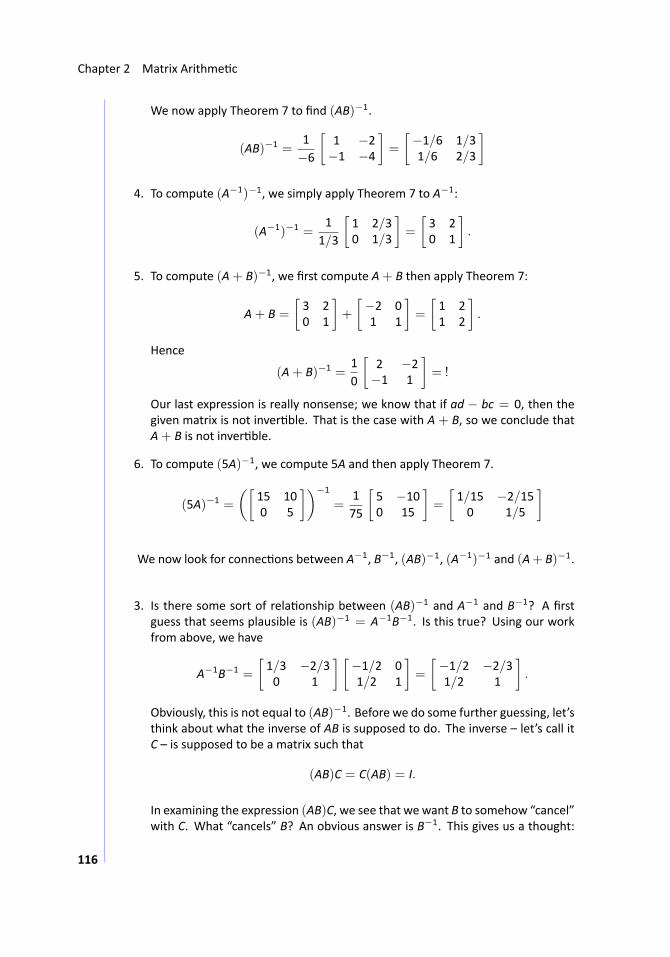
Chapter 2 Matrix Arithme c
We now apply Theorem 7 to find (AB)−1.
(AB)−1 =1−6
[1 −2−1 −4
]=
[−1/6 1/31/6 2/3
]
4. To compute (A−1)−1, we simply apply Theorem 7 to A−1:
(A−1)−1 =1
1/3
[1 2/30 1/3
]=
[3 20 1
].
5. To compute (A+ B)−1, we first compute A+ B then apply Theorem 7:
A+ B =
[3 20 1
]+
[−2 01 1
]=
[1 21 2
].
Hence
(A+ B)−1 =10
[2 −2−1 1
]= !
Our last expression is really nonsense; we know that if ad − bc = 0, then thegiven matrix is not inver ble. That is the case with A + B, so we conclude thatA+ B is not inver ble.
6. To compute (5A)−1, we compute 5A and then apply Theorem 7.
(5A)−1 =
([15 100 5
])−1
=175
[5 −100 15
]=
[1/15 −2/150 1/5
]
We now look for connec ons between A−1, B−1, (AB)−1, (A−1)−1 and (A+ B)−1...
3. Is there some sort of rela onship between (AB)−1 and A−1 and B−1? A firstguess that seems plausible is (AB)−1 = A−1B−1. Is this true? Using our workfrom above, we have
A−1B−1 =
[1/3 −2/30 1
] [−1/2 01/2 1
]=
[−1/2 −2/31/2 1
].
Obviously, this is not equal to (AB)−1. Before we do some further guessing, let’sthink about what the inverse of AB is supposed to do. The inverse – let’s call itC – is supposed to be a matrix such that
(AB)C = C(AB) = I.
In examining the expression (AB)C, we see that we want B to somehow “cancel”with C. What “cancels” B? An obvious answer is B−1. This gives us a thought:
116
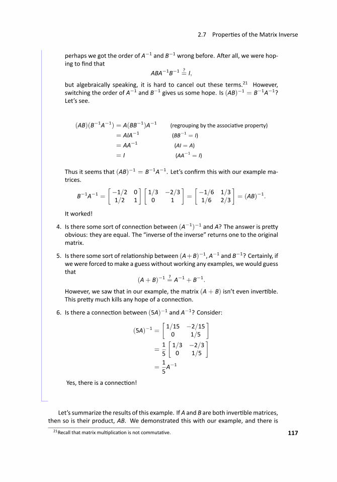
2.7 Proper es of the Matrix Inverse
perhaps we got the order of A−1 and B−1 wrong before. A er all, we were hop-ing to find that
ABA−1B−1 ?= I,
but algebraically speaking, it is hard to cancel out these terms.21 However,switching the order of A−1 and B−1 gives us some hope. Is (AB)−1 = B−1A−1?Let’s see.
(AB)(B−1A−1) = A(BB−1)A−1 (regrouping by the associa ve property)
= AIA−1 (BB−1 = I)
= AA−1 (AI = A)
= I (AA−1 = I)
Thus it seems that (AB)−1 = B−1A−1. Let’s confirm this with our example ma-trices.
B−1A−1 =
[−1/2 01/2 1
] [1/3 −2/30 1
]=
[−1/6 1/31/6 2/3
]= (AB)−1.
It worked!
4. Is there some sort of connec on between (A−1)−1 and A? The answer is pre yobvious: they are equal. The “inverse of the inverse” returns one to the originalmatrix.
5. Is there some sort of rela onship between (A+B)−1, A−1 and B−1? Certainly, ifwe were forced tomake a guess without working any examples, we would guessthat
(A+ B)−1 ?= A−1 + B−1.
However, we saw that in our example, the matrix (A + B) isn’t even inver ble.This pre y much kills any hope of a connec on.
6. Is there a connec on between (5A)−1 and A−1? Consider:
(5A)−1 =
[1/15 −2/150 1/5
]=
15
[1/3 −2/30 1/5
]=
15A−1
Yes, there is a connec on!
...
Let’s summarize the results of this example. If A and B are both inver blematrices,then so is their product, AB. We demonstrated this with our example, and there is
21Recall that matrix mul plica on is not commuta ve. 117
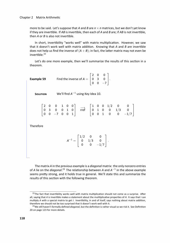
Chapter 2 Matrix Arithme c
more to be said. Let’s suppose that A and B are n× nmatrices, but we don’t yet knowif they are inver ble. If AB is inver ble, then each of A and B are; if AB is not inver ble,then A or B is also not inver ble.
In short, inver bility “works well” with matrix mul plica on. However, we sawthat it doesn’t work well with matrix addi on. Knowing that A and B are inver bledoes not help us find the inverse of (A+ B); in fact, the la er matrix may not even beinver ble.22
Let’s do one more example, then we’ll summarize the results of this sec on in atheorem.
.. Example 59 Find the inverse of A =
2 0 00 3 00 0 −7
.S We’ll find A−1 using Key Idea 10.
2 0 0 1 0 00 3 0 0 1 00 0 −7 0 0 1
−→rref
1 0 0 1/2 0 00 1 0 0 1/3 00 0 1 0 0 −1/7
Therefore
A−1 =
1/2 0 00 1/3 00 0 −1/7
.
..
ThematrixA in the previous example is a diagonalmatrix: the only nonzero entriesof A lie on the diagonal.23 The rela onship between A and A−1 in the above exampleseems pre y strong, and it holds true in general. We’ll state this and summarize theresults of this sec on with the following theorem.
22The fact that inver bility works well with matrix mul plica on should not come as a surprise. A erall, saying that A is inver ble makes a statement about the muli plica ve proper es of A. It says that I canmul ply A with a special matrix to get I. Inver bility, in and of itself, says nothing about matrix addi on,therefore we should not be too surprised that it doesn’t work well with it.
23We s ll haven’t formally defined diagonal, but the defini on is rather visual so we risk it. See Defini on20 on page 123 for more details.
118
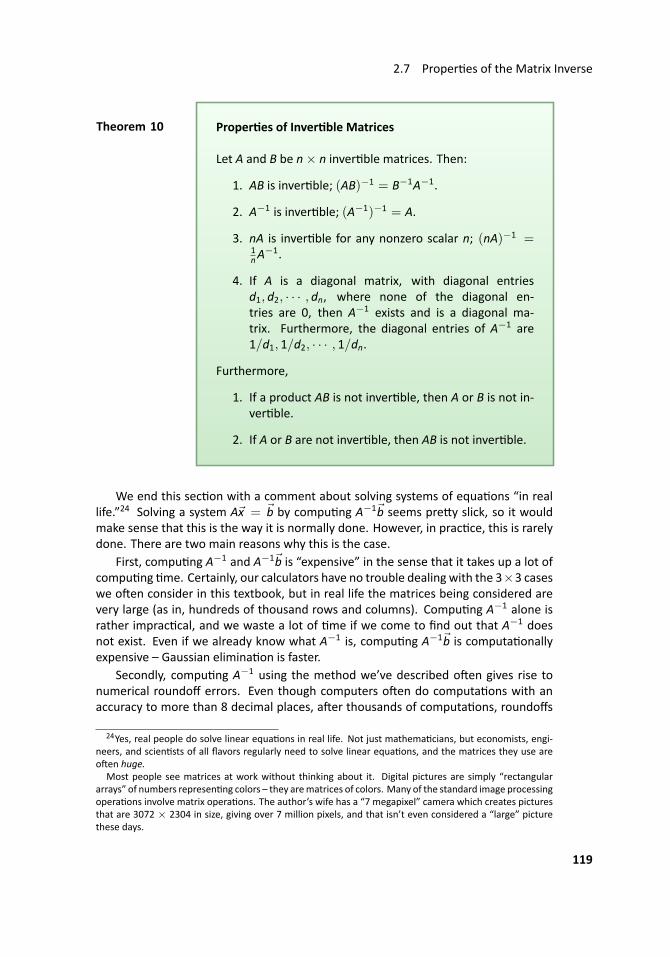
2.7 Proper es of the Matrix Inverse
..Theorem 10
.
.Proper es of Inver ble Matrices
Let A and B be n× n inver ble matrices. Then:
1. AB is inver ble; (AB)−1 = B−1A−1.
2. A−1 is inver ble; (A−1)−1 = A.
3. nA is inver ble for any nonzero scalar n; (nA)−1 =1nA
−1.
4. If A is a diagonal matrix, with diagonal entriesd1, d2, · · · , dn, where none of the diagonal en-tries are 0, then A−1 exists and is a diagonal ma-trix. Furthermore, the diagonal entries of A−1 are1/d1, 1/d2, · · · , 1/dn.
Furthermore,
1. If a product AB is not inver ble, then A or B is not in-ver ble.
2. If A or B are not inver ble, then AB is not inver ble.
We end this sec on with a comment about solving systems of equa ons “in reallife.”24 Solving a system Ax = b by compu ng A−1b seems pre y slick, so it wouldmake sense that this is the way it is normally done. However, in prac ce, this is rarelydone. There are two main reasons why this is the case.
First, compu ng A−1 and A−1b is “expensive” in the sense that it takes up a lot ofcompu ng me. Certainly, our calculators have no trouble dealing with the 3×3 caseswe o en consider in this textbook, but in real life the matrices being considered arevery large (as in, hundreds of thousand rows and columns). Compu ng A−1 alone israther imprac cal, and we waste a lot of me if we come to find out that A−1 doesnot exist. Even if we already know what A−1 is, compu ng A−1b is computa onallyexpensive – Gaussian elimina on is faster.
Secondly, compu ng A−1 using the method we’ve described o en gives rise tonumerical roundoff errors. Even though computers o en do computa ons with anaccuracy to more than 8 decimal places, a er thousands of computa ons, roundoffs
24Yes, real people do solve linear equa ons in real life. Not just mathema cians, but economists, engi-neers, and scien sts of all flavors regularly need to solve linear equa ons, and the matrices they use areo en huge.
Most people see matrices at work without thinking about it. Digital pictures are simply “rectangulararrays” of numbers represen ng colors – they arematrices of colors. Many of the standard image processingopera ons involve matrix opera ons. The author’s wife has a “7 megapixel” camera which creates picturesthat are 3072 × 2304 in size, giving over 7 million pixels, and that isn’t even considered a “large” picturethese days.
119
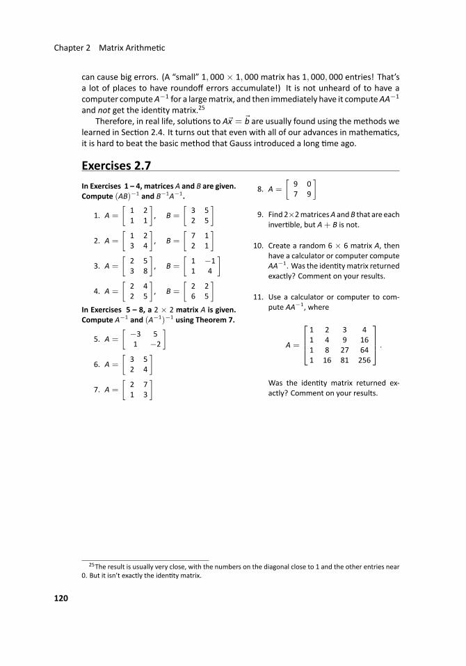
Chapter 2 Matrix Arithme c
can cause big errors. (A “small” 1, 000 × 1, 000 matrix has 1, 000, 000 entries! That’sa lot of places to have roundoff errors accumulate!) It is not unheard of to have acomputer computeA−1 for a largematrix, and then immediately have it computeAA−1
and not get the iden ty matrix.25
Therefore, in real life, solu ons to Ax = b are usually found using the methods welearned in Sec on 2.4. It turns out that even with all of our advances in mathema cs,it is hard to beat the basic method that Gauss introduced a long me ago.
Exercises 2.7In Exercises 1 – 4, matrices A and B are given.Compute (AB)−1 and B−1A−1.
1. A =
[1 21 1
], B =
[3 52 5
]2. A =
[1 23 4
], B =
[7 12 1
]3. A =
[2 53 8
], B =
[1 −11 4
]4. A =
[2 42 5
], B =
[2 26 5
]In Exercises 5 – 8, a 2 × 2 matrix A is given.Compute A−1 and (A−1)−1 using Theorem 7.
5. A =
[−3 51 −2
]6. A =
[3 52 4
]7. A =
[2 71 3
]
8. A =
[9 07 9
]9. Find 2×2matricesA andB that are each
inver ble, but A+ B is not.
10. Create a random 6 × 6 matrix A, thenhave a calculator or computer computeAA−1. Was the iden tymatrix returnedexactly? Comment on your results.
11. Use a calculator or computer to com-pute AA−1, where
A =
1 2 3 41 4 9 161 8 27 641 16 81 256
.
Was the iden ty matrix returned ex-actly? Comment on your results.
25The result is usually very close, with the numbers on the diagonal close to 1 and the other entries near0. But it isn’t exactly the iden ty matrix.
120
3 .
O M
In the previous chapter we learned about matrix arithme c: adding, subtrac ng, andmul plying matrices, finding inverses, and mul plying by scalars. In this chapter welearn about some opera ons that we perform on matrices. We can think of them asfunc ons: you input a matrix, and you get something back. One of these opera ons,the transpose, will return another matrix. With the other opera ons, the trace andthe determinant, we inputmatrices and get numbers in return, an idea that is differentthan what we have seen before.
3.1 The Matrix Transpose
...AS YOU READ . . .
1. T/F: If A is a 3× 5 matrix, then AT will be a 5× 3 matrix.
2. Where are there zeros in an upper triangular matrix?
3. T/F: A matrix is symmetric if it doesn’t change when you take its transpose.
4. What is the transpose of the transpose of A?
5. Give 2 other terms to describe symmetric matrices besides “interes ng.”
We jump right in with a defini on.
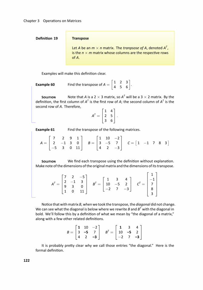
Chapter 3 Opera ons on Matrices
..Defini on 19
.
.Transpose
Let A be an m × n matrix. The tranpsose of A, denoted AT,is the n×mmatrix whose columns are the respec ve rowsof A.
Examples will make this defini on clear.
.. Example 60 Find the transpose of A =
[1 2 34 5 6
].
S Note that A is a 2 × 3 matrix, so AT will be a 3 × 2 matrix. By thedefini on, the first column of AT is the first row of A; the second column of AT is thesecond row of A. Therefore,
AT =
1 42 53 6
...
.. Example 61 Find the transpose of the following matrices.
A =
7 2 9 12 −1 3 0−5 3 0 11
B =
1 10 −23 −5 74 2 −3
C =[1 −1 7 8 3
]
S We find each transpose using the defini on without explana on.Makenote of the dimensions of the originalmatrix and the dimensions of its transpose.
AT =
7 2 −52 −1 39 3 01 0 11
BT =
1 3 410 −5 2−2 7 −3
CT =
1−1783
..
No ce thatwithmatrixB, whenwe took the transpose, thediagonal did not change.We can see what the diagonal is belowwhere we rewrite B and BT with the diagonal inbold. We’ll follow this by a defini on of what we mean by “the diagonal of a matrix,”along with a few other related defini ons.
B =
1 10 −23 –5 74 2 –3
BT =
1 3 410 –5 2−2 7 –3
It is probably pre y clear why we call those entries “the diagonal.” Here is the
formal defini on.
122
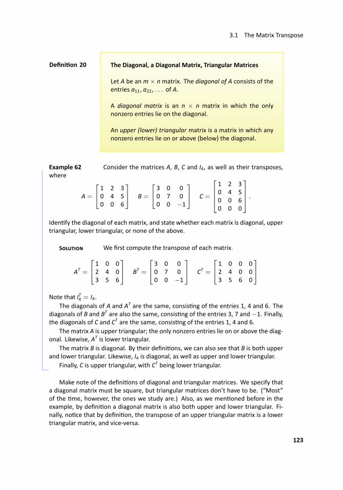
3.1 The Matrix Transpose
..Defini on 20
.
.The Diagonal, a Diagonal Matrix, Triangular Matrices
Let A be anm× nmatrix. The diagonal of A consists of theentries a11, a22, . . . of A.
A diagonal matrix is an n × n matrix in which the onlynonzero entries lie on the diagonal.
An upper (lower) triangular matrix is a matrix in which anynonzero entries lie on or above (below) the diagonal.
.. Example 62 Consider the matrices A, B, C and I4, as well as their transposes,where
A =
1 2 30 4 50 0 6
B =
3 0 00 7 00 0 −1
C =
1 2 30 4 50 0 60 0 0
.
Iden fy the diagonal of each matrix, and state whether each matrix is diagonal, uppertriangular, lower triangular, or none of the above.
S We first compute the transpose of each matrix.
AT =
1 0 02 4 03 5 6
BT =
3 0 00 7 00 0 −1
CT =
1 0 0 02 4 0 03 5 6 0
Note that IT4 = I4.
The diagonals of A and AT are the same, consis ng of the entries 1, 4 and 6. Thediagonals of B and BT are also the same, consis ng of the entries 3, 7 and−1. Finally,the diagonals of C and CT are the same, consis ng of the entries 1, 4 and 6.
The matrix A is upper triangular; the only nonzero entries lie on or above the diag-onal. Likewise, AT is lower triangular.
The matrix B is diagonal. By their defini ons, we can also see that B is both upperand lower triangular. Likewise, I4 is diagonal, as well as upper and lower triangular.
Finally, C is upper triangular, with CT being lower triangular. ..
Make note of the defini ons of diagonal and triangular matrices. We specify thata diagonal matrix must be square, but triangular matrices don’t have to be. (“Most”of the me, however, the ones we study are.) Also, as we men oned before in theexample, by defini on a diagonal matrix is also both upper and lower triangular. Fi-nally, no ce that by defini on, the transpose of an upper triangular matrix is a lowertriangular matrix, and vice-versa.
123
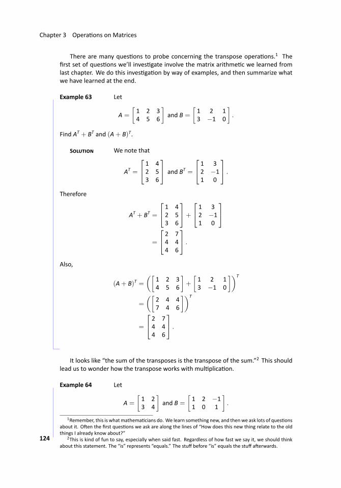
Chapter 3 Opera ons on Matrices
There are many ques ons to probe concerning the transpose opera ons.1 Thefirst set of ques ons we’ll inves gate involve the matrix arithme c we learned fromlast chapter. We do this inves ga on by way of examples, and then summarize whatwe have learned at the end.
.. Example 63 Let
A =
[1 2 34 5 6
]and B =
[1 2 13 −1 0
].
Find AT + BT and (A+ B)T.
S We note that
AT =
1 42 53 6
and BT =
1 32 −11 0
.
Therefore
AT + BT =
1 42 53 6
+
1 32 −11 0
=
2 74 44 6
.
Also,
(A+ B)T =([
1 2 34 5 6
]+
[1 2 13 −1 0
])T
=
([2 4 47 4 6
])T
=
2 74 44 6
.
..
It looks like “the sum of the transposes is the transpose of the sum.”2 This shouldlead us to wonder how the transpose works with mul plica on.
.. Example 64 ..Let
A =
[1 23 4
]and B =
[1 2 −11 0 1
].
1Remember, this is whatmathema cians do. We learn something new, and thenwe ask lots of ques onsabout it. O en the first ques ons we ask are along the lines of “How does this new thing relate to the oldthings I already know about?”
2This is kind of fun to say, especially when said fast. Regardless of how fast we say it, we should thinkabout this statement. The “is” represents “equals.” The stuff before “is” equals the stuff a erwards.
124
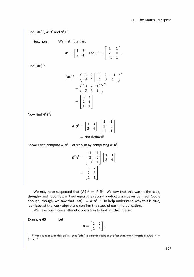
3.1 The Matrix Transpose
Find (AB)T, ATBT and BTAT.
S We first note that
AT =
[1 32 4
]and BT =
1 12 0−1 1
.
Find (AB)T:
(AB)T =([
1 23 4
] [1 2 −11 0 1
])T
=
([3 2 17 6 1
])T
=
3 72 61 1
Now find ATBT:
ATBT =
[1 32 4
] 1 12 0−1 1
= Not defined!
So we can’t compute ATBT. Let’s finish by compu ng BTAT:
BTAT =
1 12 0−1 1
[1 32 4
]
=
3 72 61 1
...
We may have suspected that (AB)T = ATBT. We saw that this wasn’t the case,though – and not onlywas it not equal, the second productwasn’t even defined! Oddlyenough, though, we saw that (AB)T = BTAT. 3 To help understand why this is true,look back at the work above and confirm the steps of each mul plica on.
We have one more arithme c opera on to look at: the inverse.
.. Example 65 ..Let
A =
[2 71 4
].
3Then again, maybe this isn’t all that “odd.” It is reminiscent of the fact that, when inver ble, (AB)−1 =B−1A−1.
125
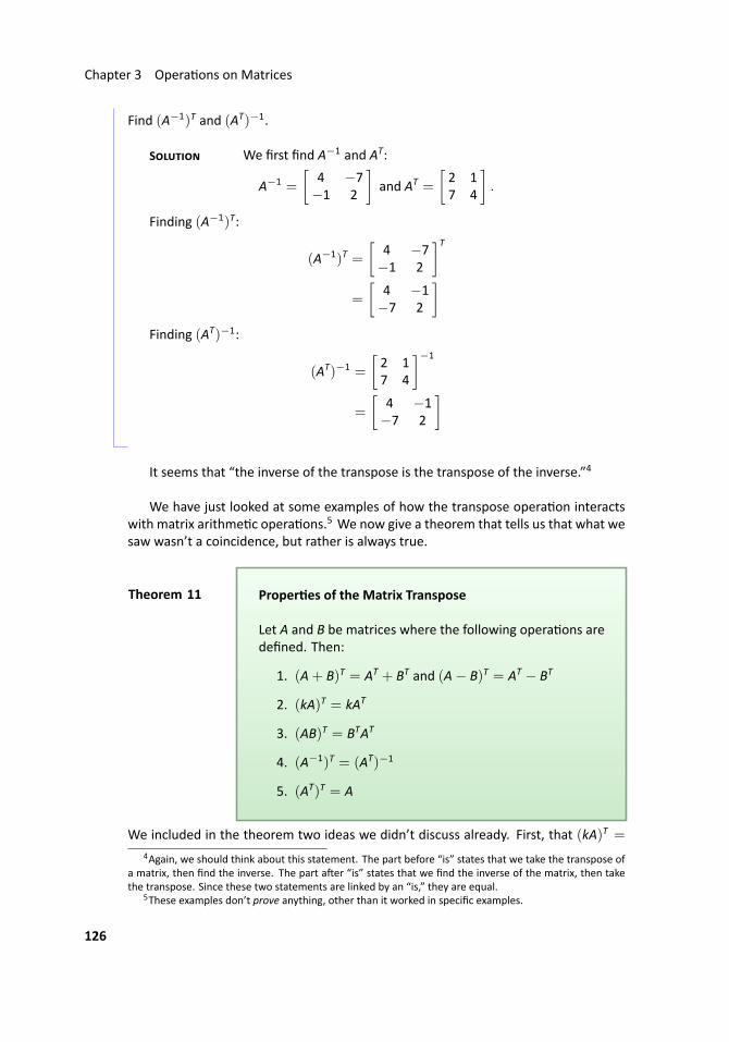
Chapter 3 Opera ons on Matrices
Find (A−1)T and (AT)−1.
S We first find A−1 and AT:
A−1 =
[4 −7−1 2
]and AT =
[2 17 4
].
Finding (A−1)T:
(A−1)T =
[4 −7−1 2
]T=
[4 −1−7 2
]Finding (AT)−1:
(AT)−1 =
[2 17 4
]−1
=
[4 −1−7 2
]...
It seems that “the inverse of the transpose is the transpose of the inverse.”4
We have just looked at some examples of how the transpose opera on interactswith matrix arithme c opera ons.5 We now give a theorem that tells us that what wesaw wasn’t a coincidence, but rather is always true.
..Theorem 11
.
.Proper es of the Matrix Transpose
Let A and B be matrices where the following opera ons aredefined. Then:
1. (A+ B)T = AT + BT and (A− B)T = AT − BT
2. (kA)T = kAT
3. (AB)T = BTAT
4. (A−1)T = (AT)−1
5. (AT)T = A
We included in the theorem two ideas we didn’t discuss already. First, that (kA)T =
4Again, we should think about this statement. The part before “is” states that we take the transpose ofa matrix, then find the inverse. The part a er “is” states that we find the inverse of the matrix, then takethe transpose. Since these two statements are linked by an “is,” they are equal.
5These examples don’t prove anything, other than it worked in specific examples.
126
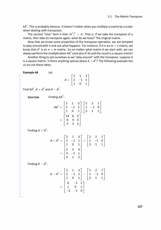
3.1 The Matrix Transpose
kAT. This is probably obvious. It doesn’t ma er when you mul ply a matrix by a scalarwhen dealing with transposes.
The second “new” item is that (AT)T = A. That is, if we take the transpose of amatrix, then take its transpose again, what do we have? The original matrix.
Now that we know some proper es of the transpose opera on, we are temptedto play around with it and see what happens. For instance, if A is anm× nmatrix, weknow that AT is an n × m matrix. So no ma er what matrix A we start with, we canalways perform themul plica on AAT (and also ATA) and the result is a square matrix!
Another thing to ask ourselves as we “play around” with the transpose: suppose Ais a square matrix. Is there anything special about A+ AT? The following example hasus try out these ideas.
.. Example 66 Let
A =
2 1 32 −1 11 0 1
.
Find AAT, A+ AT and A− AT.
S Finding AAT:
AAT =
2 1 32 −1 11 0 1
2 2 11 −1 03 1 1
=
14 6 56 4 35 3 2
Finding A+ AT:
A+ AT =
2 1 32 −1 11 0 1
+
2 2 11 −1 03 1 1
=
2 3 43 −2 14 1 2
Finding A− AT:
A− AT =
2 1 32 −1 11 0 1
−
2 2 11 −1 03 1 1
=
0 −1 21 0 1−2 −1 0
..
127
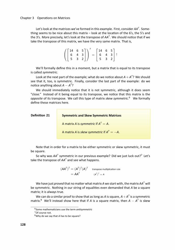
Chapter 3 Opera ons on Matrices
Let’s look at thematrices we’ve formed in this example. First, consider AAT. Some-thing seems to be nice about this matrix – look at the loca on of the 6’s, the 5’s andthe 3’s. More precisely, let’s look at the transpose of AAT. We should no ce that if wetake the transpose of this matrix, we have the very same matrix. That is, 14 6 5
6 4 35 3 2
T
=
14 6 56 4 35 3 2
!
We’ll formally define this in a moment, but a matrix that is equal to its transposeis called symmetric.
Look at the next part of the example; what do we no ce about A+AT? We shouldsee that it, too, is symmetric. Finally, consider the last part of the example: do weno ce anything about A− AT?
We should immediately no ce that it is not symmetric, although it does seem“close.” Instead of it being equal to its transpose, we no ce that this matrix is theopposite of its transpose. We call this type of matrix skew symmetric.6 We formallydefine these matrices here.
..Defini on 21
.
.Symmetric and Skew Symmetric Matrices
A matrix A is symmetric if AT = A.
A matrix A is skew symmetric if AT = −A.
Note that in order for a matrix to be either symmetric or skew symmetric, it mustbe square.
So why was AAT symmetric in our previous example? Did we just luck out?7 Let’stake the transpose of AAT and see what happens.
(AAT)T = (AT)T(A)T transpose mul plica on rule
= AAT(AT
)T= A
Wehave just proved that noma erwhatmatrixAwe start with, thematrixAAT willbe symmetric. Nothing in our string of equali es even demanded that A be a squarematrix; it is always true.
We can do a similar proof to show that as long as A is square, A+AT is a symmetricmatrix.8 We’ll instead show here that if A is a square matrix, then A − AT is skew
6Some mathema cians use the term an symmetric7Of course not.8Why do we say that A has to be square?
128
3.1 The Matrix Transpose
symmetric.
(A− AT)T = AT − (AT)T transpose subtrac on rule
= AT − A
= −(A− AT)
So we took the transpose of A− AT and we got−(A− AT); this is the defini on ofbeing skew symmetric.
We’ll take what we learned from Example 66 and put it in a box. (We’ve alreadyproved most of this is true; the rest we leave to solve in the Exercises.)
..Theorem 12
.
.Symmetric and Skew Symmetric Matrices
1. Given anymatrixA, thematricesAAT andATA are sym-metric.
2. Let A be a square matrix. The matrix A + AT is sym-metric.
3. Let A be a square matrix. The matrix A − AT is skewsymmetric.
Why dowe care about the transpose of amatrix? Why dowe care about symmetricmatrices?
There are two answers that each answer both of these ques ons. First, we areinterested in the tranpose of a matrix and symmetric matrices because they are in-teres ng.9 One par cularly interes ng thing about symmetric and skew symmetricmatrices is this: consider the sum of (A+ AT) and (A− AT):
(A+ AT) + (A− AT) = 2A.
This gives us an idea: if we were to mul ply both sides of this equa on by 12 , then the
right hand side would just be A. This means that
A =12(A+ AT)︸ ︷︷ ︸symmetric
+12(A− AT)︸ ︷︷ ︸
skew symmetric
.
That is, any matrix A can be wri en as the sum of a symmetric and skew symmetricmatrix. That’s interes ng.
The second reasonwe care about them is that they are very useful and important invarious areas of mathema cs. The transpose of a matrix turns out to be an important
9Or: “neat,” “cool,” “bad,” “wicked,” “phat,” “fo-shizzle.”
129
Chapter 3 Opera ons on Matrices
opera on; symmetric matrices have many nice proper es that make solving certaintypes of problems possible.
Most of this text focuses on the preliminaries ofmatrix algebra, and the actual usesare beyond our current scope. One easy to describe example is curve fi ng. Supposewe are given a large set of data points that, when plo ed, look roughly quadra c. Howdo we find the quadra c that “best fits” this data? The solu on can be found usingmatrix algebra, and specifically a matrix called the pseudoinverse. If A is a matrix, thepseudoinverse of A is the matrix A† = (ATA)−1AT (assuming that the inverse exists).We aren’t going to worry about what all the abovemeans; just no ce that it has a coolsounding name and the transpose appears twice.
In the next sec on we’ll learn about the trace, another opera on that can be per-formed on a matrix that is rela vely simple to compute but can lead to some deepresults.
Exercises 3.1In Exercises 1 – 24, a matrix A is given. FindAT; make note if A is upper/lower triangular,diagonal, symmetric and/or skew symmetric.
1.[−7 44 −6
]2.
[3 1−7 8
]3.
[1 00 9
]4.
[13 −3−3 1
]
5.
−5 −93 1
−10 −8
6.
−2 101 −79 −2
7.
[4 −7 −4 −9−9 6 3 −9
]8.
[3 −10 0 6
−10 −2 −3 1
]9.
[−7 −8 2 −3
]10.
[−9 8 2 −7
]11.
−9 4 106 −3 −7−8 1 −1
12.
4 −5 21 5 99 2 3
13.
4 0 −20 2 3−2 3 6
14.
0 3 −23 −4 1−2 1 0
15.
2 −5 −35 5 −67 −4 −10
16.
0 −6 16 0 4−1 −4 0
17.
4 2 −95 −4 −10−6 6 9
18.
4 0 0−2 −7 04 −2 5
19.
−3 −4 −50 −3 50 0 −3
20.
6 −7 2 60 −8 −1 00 0 1 −7
130
3.2 The Matrix Trace
21.
1 0 00 2 00 0 −1
22.
6 −4 −5−4 0 2−5 2 −2
23.
0 1 −2−1 0 42 −4 0
24.
0 0 00 0 00 0 0
3.2 The Matrix Trace...AS YOU READ . . .
1. T/F: We only compute the trace of square matrices.
2. T/F: One can tell if a matrix is inver ble by compu ng the trace.
In the previous sec on, we learned about an opera onwe can peformonmatrices,namely the transpose. Given a matrix A, we can “find the transpose of A,” which isanother matrix. In this sec on we learn about a new opera on called the trace. It isa different type of opera on than the transpose. Given a matrix A, we can “find thetrace of A,” which is not a matrix but rather a number. We formally define it here.
..Defini on 22
.
.The Trace
Let A be an n × n matrix. The trace of A, denoted tr(A), isthe sum of the diagonal elements of A. That is,
tr(A) = a11 + a22 + · · ·+ ann.
This seems like a simple defini on, and it really is. Just to make sure it is clear, let’sprac ce.
.. Example 67 ..Find the trace of A, B, C and I4, where
A =
[1 23 4
], B =
1 2 03 8 1−2 7 −5
and C =
[1 2 34 5 6
].
S To find the trace of A, note that the diagonal elements of A are 1and 4. Therefore, tr(A) = 1+ 4 = 5.
We see that the diagonal elements of B are 1, 8 and -5, so tr(B)= 1+ 8− 5 = 4.
131
Chapter 3 Opera ons on Matrices
The matrix C is not a square matrix, and our defini on states that we must startwith a square matrix. Therefore tr(C) is not defined.
Finally, the diagonal of I4 consists of four 1s. Therefore tr(I4) = 4. ...
Now that we have defined the trace of a matrix, we should think like mathema -cians and ask some ques ons. The first ques ons that should pop into our mindsshould be along the lines of “Howdoes the traceworkwith othermatrix opera ons?”10
We should think about how the trace works withmatrix addi on, scalar mul plica on,matrix mul plica on, matrix inverses, and the transpose.
We’ll give a theorem that will formally tell us what is true in a moment, but firstlet’s play with two sample matrices and see if we can see what will happen. Let
A =
2 1 32 0 −13 −1 3
and B =
2 0 1−1 2 00 2 −1
.
It should be clear that tr(A) = 5 and tr(B) = 3. What is tr(A+ B)?
tr(A+ B) = tr
2 1 32 0 −13 −1 3
+
2 0 1−1 2 00 2 −1
= tr
4 1 41 2 −13 1 2
= 8
So we no ce that tr(A+ B) = tr(A) + tr(B). This probably isn’t a coincidence.
How does the trace work with scalar mul plica on? If wemul ply A by 4, then thediagonal elements will be 8, 0 and 12, so tr(4A) = 20. Is it a coincidence that this is 4mes the trace of A?
Let’s move on tomatrix mul plica on. Howwill the trace of AB relate to the tracesof A and B? Let’s see:
tr(AB) = tr
2 1 32 0 −13 −1 3
2 0 1−1 2 00 2 −1
= tr
3 8 −14 −2 37 4 0
= 1
10Recall that we asked a similar ques on once we learned about the transpose.
132
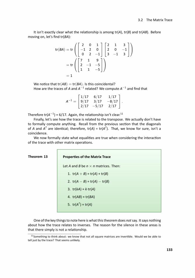
3.2 The Matrix Trace
It isn’t exactly clear what the rela onship is among tr(A), tr(B) and tr(AB). Beforemoving on, let’s find tr(BA):
tr(BA) = tr
2 0 1−1 2 00 2 −1
2 1 32 0 −13 −1 3
= tr
7 1 92 −1 −51 1 −5
= 1
We no ce that tr(AB) = tr(BA). Is this coincidental?How are the traces of A and A−1 related? We compute A−1 and find that
A−1 =
1/17 6/17 1/179/17 3/17 −8/172/17 −5/17 2/17
.
Therefore tr(A−1) = 6/17. Again, the rela onship isn’t clear.11
Finally, let’s see how the trace is related to the transpose. We actually don’t haveto formally compute anything. Recall from the previous sec on that the diagonalsof A and AT are iden cal; therefore, tr(A) = tr(AT). That, we know for sure, isn’t acoincidence.
We now formally state what equali es are true when considering the interac onof the trace with other matrix opera ons.
..Theorem 13
.
.Proper es of the Matrix Trace
Let A and B be n× nmatrices. Then:
1. tr(A+ B) = tr(A) + tr(B)
2. tr(A− B) = tr(A)− tr(B)
3. tr(kA) = k·tr(A)
4. tr(AB) = tr(BA)
5. tr(AT) = tr(A)
One of the key things to note here iswhat this theoremdoes not say. It says nothingabout how the trace relates to inverses. The reason for the silence in these areas isthat there simply is not a rela onship.
11Something to think about: we know that not all square matrices are inver ble. Would we be able totell just by the trace? That seems unlikely.
133
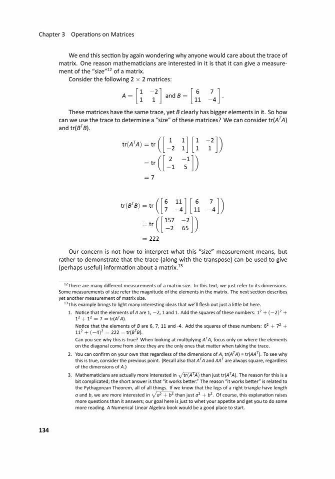
Chapter 3 Opera ons on Matrices
We end this sec on by again wondering why anyone would care about the trace ofmatrix. One reason mathema cians are interested in it is that it can give a measure-ment of the “size”12 of a matrix.
Consider the following 2× 2 matrices:
A =
[1 −21 1
]and B =
[6 711 −4
].
Thesematrices have the same trace, yet B clearly has bigger elements in it. So howcan we use the trace to determine a “size” of these matrices? We can consider tr(ATA)and tr(BTB).
tr(ATA) = tr([
1 1−2 1
] [1 −21 1
])= tr
([2 −1−1 5
])= 7
tr(BTB) = tr([
6 117 −4
] [6 711 −4
])= tr
([157 −2−2 65
])= 222
Our concern is not how to interpret what this “size” measurement means, butrather to demonstrate that the trace (along with the transpose) can be used to give(perhaps useful) informa on about a matrix.13
12There are many different measurements of a matrix size. In this text, we just refer to its dimensions.Some measurements of size refer the magnitude of the elements in the matrix. The next sec on describesyet another measurement of matrix size.
13This example brings to light many interes ng ideas that we’ll flesh out just a li le bit here.
1. No ce that the elements of A are 1,−2, 1 and 1. Add the squares of these numbers: 12 +(−2)2 +12 + 12 = 7 = tr(ATA).No ce that the elements of B are 6, 7, 11 and -4. Add the squares of these numbers: 62 + 72 +112 + (−4)2 = 222 = tr(BTB).Can you see why this is true? When looking at mul plying ATA, focus only on where the elementson the diagonal come from since they are the only ones that ma er when taking the trace.
2. You can confirm on your own that regardless of the dimensions of A, tr(ATA) = tr(AAT). To see whythis is true, consider the previous point. (Recall also that ATA and AAT are always square, regardlessof the dimensions of A.)
3. Mathema cians are actually more interested in√
tr(ATA) than just tr(ATA). The reason for this is abit complicated; the short answer is that “it works be er.” The reason “it works be er” is related tothe Pythagorean Theorem, all of all things. If we know that the legs of a right triangle have lengtha and b, we are more interested in
√a2 + b2 than just a2 + b2. Of course, this explana on raises
more ques ons than it answers; our goal here is just to whet your appe te and get you to do somemore reading. A Numerical Linear Algebra book would be a good place to start.
134
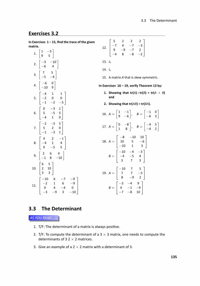
3.3 The Determinant
Exercises 3.2In Exercises 1 – 15, find the trace of the givenmatrix.
1.[1 −59 5
]2.
[−3 −10−6 4
]3.
[7 5−5 −4
]4.
[−6 0−10 9
]
5.
−4 1 1−2 0 0−1 −2 −5
6.
0 −3 15 −5 5−4 1 0
7.
−2 −3 55 2 0−1 −3 1
8.
4 2 −1−4 1 40 −5 5
9.
[2 6 4−1 8 −10
]
10.
6 52 103 3
11.
−10 6 −7 −9−2 1 6 −90 4 −4 0−3 −9 3 −10
12.
5 2 2 2−7 4 −7 −39 −9 −7 2−4 8 −8 −2
13. I4
14. In
15. A matrix A that is skew symmetric.
In Exercises 16 – 19, verify Theorem 13 by:
1. Showing that tr(A)+tr(B) = tr(A + B)and
2. Showing that tr(AB) = tr(BA).
16. A =
[1 −19 −6
], B =
[−1 0−6 3
]
17. A =
[0 −81 8
], B =
[−4 5−4 2
]
18. A =
−8 −10 1010 5 −6−10 1 3
B =
−10 −4 −3−4 −5 43 7 3
19. A =
−10 7 57 7 −58 −9 2
B =
−3 −4 94 −1 −9−7 −8 10
3.3 The Determinant...AS YOU READ . . .
1. T/F: The determinant of a matrix is always posi ve.
2. T/F: To compute the determinant of a 3 × 3 matrix, one needs to compute thedeterminants of 3 2× 2 matrices.
3. Give an example of a 2× 2 matrix with a determinant of 3.
135
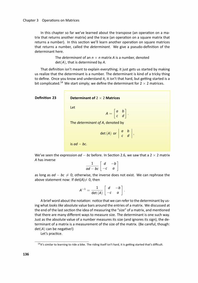
Chapter 3 Opera ons on Matrices
In this chapter so far we’ve learned about the transpose (an opera on on a ma-trix that returns another matrix) and the trace (an opera on on a square matrix thatreturns a number). In this sec on we’ll learn another opera on on square matricesthat returns a number, called the determinant. We give a pseudo-defini on of thedeterminant here.
The determinant of an n× nmatrix A is a number, denoteddet(A), that is determined by A.
That defini on isn’t meant to explain everything; it just gets us started by makingus realize that the determinant is a number. The determinant is kind of a tricky thingto define. Once you know and understand it, it isn’t that hard, but ge ng started is abit complicated.14 We start simply; we define the determinant for 2× 2 matrices.
..Defini on 23
.
.Determinant of 2× 2Matrices
Let
A =
[a bc d
].
The determinant of A, denoted by
det (A) or
∣∣∣∣ a bc d
∣∣∣∣ ,is ad− bc.
We’ve seen the expression ad− bc before. In Sec on 2.6, we saw that a 2× 2 matrixA has inverse
1ad− bc
[d −b−c a
]as long as ad − bc = 0; otherwise, the inverse does not exist. We can rephrase theabove statement now: If det(A) = 0, then
A−1 =1
det (A)
[d −b−c a
].
A brief word about the nota on: no ce that we can refer to the determinant by us-ing what looks like absolute value bars around the entries of a matrix. We discussed atthe end of the last sec on the idea of measuring the “size” of a matrix, andmen onedthat there are many different ways to measure size. The determinant is one such way.Just as the absolute value of a number measures its size (and ignores its sign), the de-terminant of a matrix is a measurement of the size of the matrix. (Be careful, though:det(A) can be nega ve!)
Let’s prac ce.
14It’s similar to learning to ride a bike. The riding itself isn’t hard, it is ge ng started that’s difficult.
136
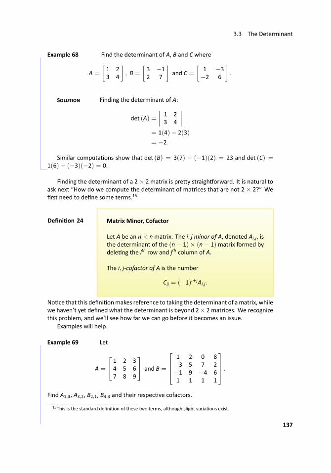
3.3 The Determinant
.. Example 68 Find the determinant of A, B and C where
A =
[1 23 4
], B =
[3 −12 7
]and C =
[1 −3−2 6
].
S Finding the determinant of A:
det (A) =
∣∣∣∣ 1 23 4
∣∣∣∣= 1(4)− 2(3)
= −2.
Similar computa ons show that det (B) = 3(7) − (−1)(2) = 23 and det (C) =1(6)− (−3)(−2) = 0. ..
Finding the determinant of a 2× 2 matrix is pre y straigh orward. It is natural toask next “How do we compute the determinant of matrices that are not 2 × 2?” Wefirst need to define some terms.15
..Defini on 24
.
.Matrix Minor, Cofactor
Let A be an n× nmatrix. The i, j minor of A, denoted Ai,j, isthe determinant of the (n− 1)× (n− 1)matrix formed bydele ng the ith row and jth column of A.
The i, j-cofactor of A is the number
Cij = (−1)i+jAi,j.
No ce that this defini onmakes reference to taking the determinant of amatrix, whilewe haven’t yet defined what the determinant is beyond 2× 2 matrices. We recognizethis problem, and we’ll see how far we can go before it becomes an issue.
Examples will help.
.. Example 69 ..Let
A =
1 2 34 5 67 8 9
and B =
1 2 0 8−3 5 7 2−1 9 −4 61 1 1 1
.
Find A1,3, A3,2, B2,1, B4,3 and their respec ve cofactors.
15This is the standard defini on of these two terms, although slight varia ons exist.
137
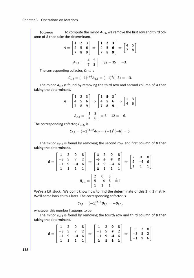
Chapter 3 Opera ons on Matrices
S To compute the minor A1,3, we remove the first row and third col-umn of A then take the determinant.
A =
1 2 34 5 67 8 9
⇒
1 2 34 5 67 8 9
⇒[4 57 8
]
A1,3 =
∣∣∣∣ 4 57 8
∣∣∣∣ = 32− 35 = −3.
The corresponding cofactor, C1,3, is
C1,3 = (−1)1+3A1,3 = (−1)4(−3) = −3.
The minor A3,2 is found by removing the third row and second column of A thentaking the determinant.
A =
1 2 34 5 67 8 9
⇒
1 2 34 5 67 8 9
⇒[1 34 6
]
A3,2 =
∣∣∣∣ 1 34 6
∣∣∣∣ = 6− 12 = −6.
The corresponding cofactor, C3,2, is
C3,2 = (−1)3+2A3,2 = (−1)5(−6) = 6.
..The minor B2,1 is found by removing the second row and first column of B then
taking the determinant.
B =
1 2 0 8−3 5 7 2−1 9 −4 61 1 1 1
⇒
1 2 0 8-3 5 7 2-1 9 −4 61 1 1 1
⇒
2 0 89 −4 61 1 1
B2,1 =
∣∣∣∣∣∣2 0 89 −4 61 1 1
∣∣∣∣∣∣ != ?
We’re a bit stuck. We don’t know how to find the determinate of this 3 × 3 matrix.We’ll come back to this later. The corresponding cofactor is
C2,1 = (−1)2+1B2,1 = −B2,1,
whatever this number happens to be.The minor B4,3 is found by removing the fourth row and third column of B then
taking the determinant.
B =
1 2 0 8−3 5 7 2−1 9 −4 61 1 1 1
⇒
1 2 0 8−3 5 7 2−1 9 -4 61 1 1 1
⇒
1 2 8−3 5 2−1 9 6
138
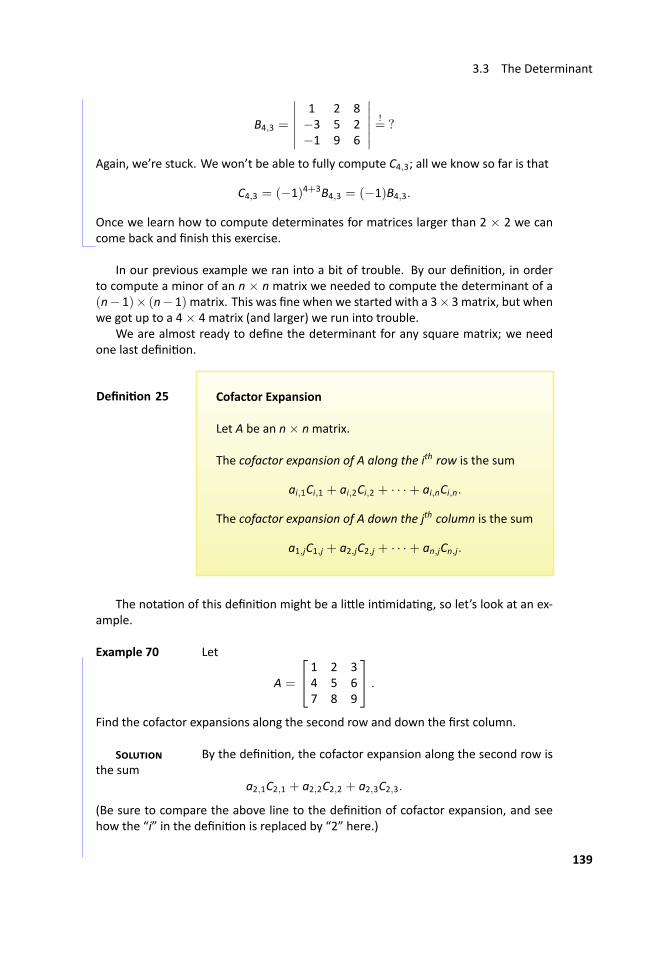
3.3 The Determinant
B4,3 =
∣∣∣∣∣∣1 2 8−3 5 2−1 9 6
∣∣∣∣∣∣ != ?
Again, we’re stuck. We won’t be able to fully compute C4,3; all we know so far is that
C4,3 = (−1)4+3B4,3 = (−1)B4,3.
Once we learn how to compute determinates for matrices larger than 2 × 2 we cancome back and finish this exercise. ...
In our previous example we ran into a bit of trouble. By our defini on, in orderto compute a minor of an n × n matrix we needed to compute the determinant of a(n− 1)× (n− 1)matrix. This was fine when we started with a 3× 3 matrix, but whenwe got up to a 4× 4 matrix (and larger) we run into trouble.
We are almost ready to define the determinant for any square matrix; we needone last defini on.
..Defini on 25
.
.Cofactor Expansion
Let A be an n× nmatrix.
The cofactor expansion of A along the ith row is the sum
ai,1Ci,1 + ai,2Ci,2 + · · ·+ ai,nCi,n.
The cofactor expansion of A down the jth column is the sum
a1,jC1,j + a2,jC2,j + · · ·+ an,jCn,j.
The nota on of this defini on might be a li le in mida ng, so let’s look at an ex-ample.
.. Example 70 ..Let
A =
1 2 34 5 67 8 9
.
Find the cofactor expansions along the second row and down the first column.
S By the defini on, the cofactor expansion along the second row isthe sum
a2,1C2,1 + a2,2C2,2 + a2,3C2,3.
(Be sure to compare the above line to the defini on of cofactor expansion, and seehow the “i” in the defini on is replaced by “2” here.)
139
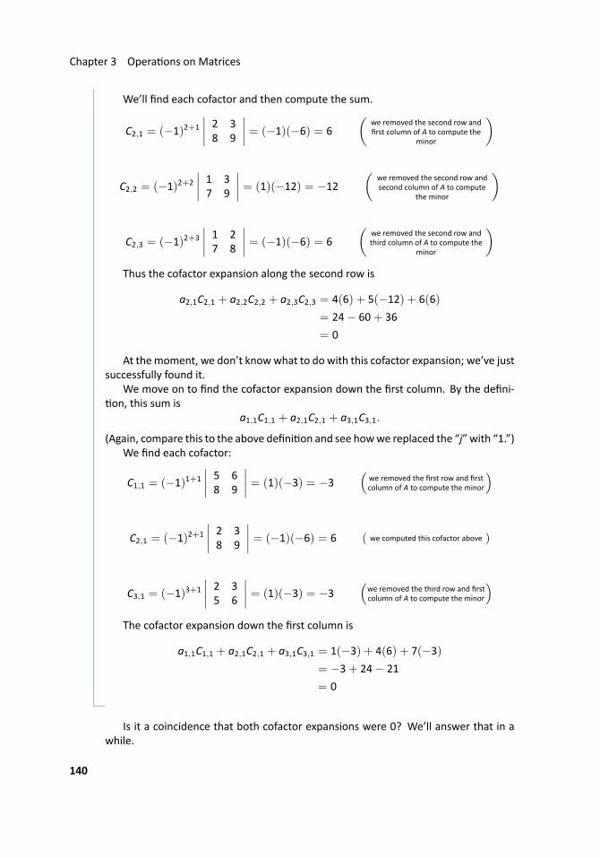
Chapter 3 Opera ons on Matrices
We’ll find each cofactor and then compute the sum.
C2,1 = (−1)2+1
∣∣∣∣ 2 38 9
∣∣∣∣ = (−1)(−6) = 6(
we removed the second row andfirst column of A to compute the
minor
)
C2,2 = (−1)2+2
∣∣∣∣ 1 37 9
∣∣∣∣ = (1)(−12) = −12(
we removed the second row andsecond column of A to compute
the minor
)
C2,3 = (−1)2+3
∣∣∣∣ 1 27 8
∣∣∣∣ = (−1)(−6) = 6(
we removed the second row andthird column of A to compute the
minor
)Thus the cofactor expansion along the second row is
a2,1C2,1 + a2,2C2,2 + a2,3C2,3 = 4(6) + 5(−12) + 6(6)
= 24− 60+ 36
= 0
At themoment, we don’t knowwhat to do with this cofactor expansion; we’ve justsuccessfully found it.
We move on to find the cofactor expansion down the first column. By the defini-on, this sum is
a1,1C1,1 + a2,1C2,1 + a3,1C3,1.
(Again, compare this to the above defini on and see howwe replaced the “j” with “1.”)We find each cofactor:
C1,1 = (−1)1+1
∣∣∣∣ 5 68 9
∣∣∣∣ = (1)(−3) = −3(
we removed the first row and firstcolumn of A to compute the minor
)
C2,1 = (−1)2+1
∣∣∣∣ 2 38 9
∣∣∣∣ = (−1)(−6) = 6 ( we computed this cofactor above )
C3,1 = (−1)3+1
∣∣∣∣ 2 35 6
∣∣∣∣ = (1)(−3) = −3(we removed the third row and firstcolumn of A to compute the minor
)The cofactor expansion down the first column is
a1,1C1,1 + a2,1C2,1 + a3,1C3,1 = 1(−3) + 4(6) + 7(−3)
= −3+ 24− 21
= 0...
Is it a coincidence that both cofactor expansions were 0? We’ll answer that in awhile.
140
3.3 The Determinant
This sec on is en tled “The Determinant,” yet we don’t know how to compute ityet except for 2× 2 matrices. We finally define it now.
..Defini on 26
.
.The Determinant
The determinant of an n×nmatrix A, denoted det(A) or |A|,is a number given by the following:
• if A is a 1× 1 matrix A = [a], then det (A) = a.
• if A is a 2× 2 matrix
A =
[a bc d
],
then det (A) = ad− bc.
• if A is an n×nmatrix, where n ≥ 2, then det(A) is thenumber found by taking the cofactor expansion alongthe first row of A. That is,
det (A) = a1,1C1,1 + a1,2C1,2 + · · ·+ a1,nC1,n.
No ce that in order to compute the determinant of an n× nmatrix, we need to com-pute the determinants of n (n− 1)× (n− 1)matrices. This can be a lot of work. We’lllater learn how to shorten some of this. First, let’s prac ce.
.. Example 71 ..Find the determinant of
A =
1 2 34 5 67 8 9
.
S No ce that this is the matrix from Example 70. The cofactor ex-pansion along the first row is
det (A) = a1,1C1,1 + a1,2C1,2 + a1,3C1,3.
We’ll compute each cofactor first then take the appropriate sum.
141
Chapter 3 Opera ons on Matrices
C1,1 = (−1)1+1A1,1
= 1 ·∣∣∣∣ 5 68 9
∣∣∣∣= 45− 48
= −3
C1,2 = (−1)1+2A1,2
= (−1) ·∣∣∣∣ 4 67 9
∣∣∣∣= (−1)(36− 42)
= 6
C1,3 = (−1)1+3A1,3
= 1 ·∣∣∣∣ 4 57 8
∣∣∣∣= 32− 35
= −3
Therefore the determinant of A is
det (A) = 1(−3) + 2(6) + 3(−3) = 0....
.. Example 72 Find the determinant of
A =
3 6 70 2 −13 −1 1
.
S We’ll compute each cofactor first then find the determinant.
C1,1 = (−1)1+1A1,1
= 1 ·∣∣∣∣ 2 −1−1 1
∣∣∣∣= 2− 1
= 1
C1,2 = (−1)1+2A1,2
= (−1) ·∣∣∣∣ 0 −13 1
∣∣∣∣= (−1)(0+ 3)
= −3
C1,3 = (−1)1+3A1,3
= 1 ·∣∣∣∣ 0 23 −1
∣∣∣∣= 0− 6
= −6
Thus the determinant is
det (A) = 3(1) + 6(−3) + 7(−6) = −57...
.. Example 73 ..Find the determinant of
A =
1 2 1 2−1 2 3 48 5 −3 15 9 −6 3
.
S This, quite frankly, will take quite a bit ofwork. In order to computethis determinant, we need to compute 4 minors, each of which requires finding thedeterminant of a 3× 3 matrix! Complaining won’t get us any closer to the solu on,16
16But it might make us feel a li le be er. Glance ahead: do you see how much work we have to do?!?
142
3.3 The Determinant
so let’s get started. We first compute the cofactors:
C1,1 = (−1)1+1A1,1
= 1 ·
∣∣∣∣∣∣2 3 45 −3 19 −6 3
∣∣∣∣∣∣ (we must compute the determinantof this 3 × 3 matrix
)= 2 · (−1)1+1
∣∣∣∣ −3 1−6 3
∣∣∣∣+ 3 · (−1)1+2
∣∣∣∣ 5 19 3
∣∣∣∣+ 4 · (−1)1+3
∣∣∣∣ 5 −39 −6
∣∣∣∣= 2(−3) + 3(−6) + 4(−3)
= −36
C1,2 = (−1)1+2A1,2
= (−1) ·
∣∣∣∣∣∣−1 3 48 −3 15 −6 3
∣∣∣∣∣∣ (we must compute the determinantof this 3 × 3 matrix
)= (−1)
[(−1) · (−1)1+1
∣∣∣∣ −3 1−6 3
∣∣∣∣+ 3 · (−1)1+2
∣∣∣∣ 8 15 3
∣∣∣∣+ 4 · (−1)1+3
∣∣∣∣ 8 −35 −6
∣∣∣∣]︸ ︷︷ ︸the determinate of the 3 × 3 matrix
= (−1) [(−1)(−3) + 3(−19) + 4(−33)]
= 186
..
C1,3 = (−1)1+3A1,3
= 1 ·
∣∣∣∣∣∣−1 2 48 5 15 9 3
∣∣∣∣∣∣ (we must compute the determinantof this 3 × 3 matrix
)= (−1) · (−1)1+1
∣∣∣∣ 5 19 3
∣∣∣∣+ 2 · (−1)1+2
∣∣∣∣ 8 15 3
∣∣∣∣+ 4 · (−1)1+3
∣∣∣∣ 8 55 9
∣∣∣∣= (−1)(6) + 2(−19) + 4(47)
= 144
143
Chapter 3 Opera ons on Matrices
C1,4 = (−1)1+4A1,4
= (−1) ·
∣∣∣∣∣∣−1 2 38 5 −35 9 −6
∣∣∣∣∣∣ (we must compute the determinantof this 3 × 3 matrix
)= (−1)
[(−1) · (−1)1+1
∣∣∣∣ 5 −39 −6
∣∣∣∣+ 2 · (−1)1+2
∣∣∣∣ 8 −35 −6
∣∣∣∣+ 3 · (−1)1+3
∣∣∣∣ 8 55 9
∣∣∣∣]︸ ︷︷ ︸the determinate of the 3 × 3 matrix
= (−1) [(−1)(−3) + 2(33) + 3(47)]
= −210
We’ve computed our four cofactors. All that is le is to compute the cofactor ex-pansion.
det (A) = 1(−36) + 2(186) + 1(144) + 2(−210) = 60.
As a way of “visualizing” this, let’s write out the cofactor expansion again but in-cluding the matrices in their place.
det (A) = a1,1C1,1 + a1,2C1,2 + a1,3C1,3 + a1,4C1,4
= 1(−1)2
∣∣∣∣∣∣2 3 45 −3 19 −6 3
∣∣∣∣∣∣︸ ︷︷ ︸= −36
+ 2(−1)3
∣∣∣∣∣∣−1 3 48 −3 15 −6 3
∣∣∣∣∣∣︸ ︷︷ ︸= −186
+
1(−1)4
∣∣∣∣∣∣−1 2 48 5 15 9 3
∣∣∣∣∣∣︸ ︷︷ ︸= 144
+ 2(−1)5
∣∣∣∣∣∣−1 2 38 5 −35 9 −6
∣∣∣∣∣∣︸ ︷︷ ︸= 210
= 60...
That certainly took a while; it required more than 50 mul plica ons (we didn’tcount the addi ons). To compute the determinant of a 5 × 5 matrix, we’ll need tocompute the determinants of five 4 × 4 matrices, meaning that we’ll need over 250mul plica ons! Not only is this a lot of work, but there are just toomanyways tomakesilly mistakes.17 There are some tricks to make this job easier, but regardless we seethe need to employ technology. Even then, technology quickly bogs down. A 25× 25matrix is considered “small” by today’s standards,18 but it is essen ally impossible fora computer to compute its determinant by only using cofactor expansion; it too needsto employ “tricks.”
17The author made three when the above example was originally typed.18It is common for mathema cians, scien sts and engineers to consider linear systems with thousands
of equa ons and variables.
144
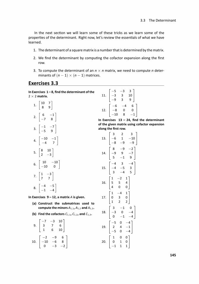
3.3 The Determinant
In the next sec on we will learn some of these tricks as we learn some of theproper es of the determinant. Right now, let’s review the essen als of what we havelearned.
1. The determinant of a squarematrix is a number that is determinedby thematrix.
2. We find the determinant by compu ng the cofactor expansion along the firstrow.
3. To compute the determinant of an n × n matrix, we need to compute n deter-minants of (n− 1)× (n− 1)matrices.
Exercises 3.3In Exercises 1 – 8, find the determinant of the2× 2matrix.
1.[10 78 9
]
2.[
6 −1−7 8
]
3.[−1 −7−5 9
]
4.[−10 −1−4 7
]
5.[8 102 −3
]
6.[
10 −10−10 0
]
7.[1 −37 7
]
8.[−4 −5−1 −4
]In Exercises 9 – 12, a matrix A is given.
(a) Construct the submatrices used tocompute theminors A1,1, A1,2 and A1,3.
(b) Find the cofactors C1,1, C1,2, and C1,3.
9.
−7 −3 103 7 61 6 10
10.
−2 −9 6−10 −6 80 −3 −2
11.
−5 −3 3−3 3 10−9 3 9
12.
−6 −4 6−8 0 0−10 8 −1
In Exercises 13 – 24, find the determinantof the given matrix using cofactor expansionalong the first row.
13.
3 2 3−6 1 −10−8 −9 −9
14.
8 −9 −2−9 9 −75 −1 9
15.
−4 3 −4−4 −5 33 −4 5
16.
1 −2 15 5 44 0 0
17.
1 −4 10 3 01 2 2
18.
3 −1 0−3 0 −40 −1 −4
19.
−5 0 −42 4 −1−5 0 −4
20.
1 0 00 1 0−1 1 1
145
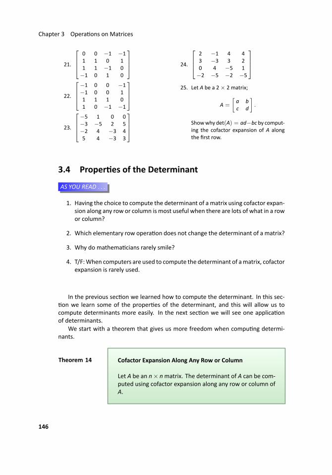
Chapter 3 Opera ons on Matrices
21.
0 0 −1 −11 1 0 11 1 −1 0−1 0 1 0
22.
−1 0 0 −1−1 0 0 11 1 1 01 0 −1 −1
23.
−5 1 0 0−3 −5 2 5−2 4 −3 45 4 −3 3
24.
2 −1 4 43 −3 3 20 4 −5 1−2 −5 −2 −5
25. Let A be a 2× 2 matrix;
A =
[a bc d
].
Showwhy det(A) = ad−bc by comput-ing the cofactor expansion of A alongthe first row.
3.4 Proper es of the Determinant
...AS YOU READ . . .
1. Having the choice to compute the determinant of amatrix using cofactor expan-sion along any row or column is most useful when there are lots of what in a rowor column?
2. Which elementary row opera on does not change the determinant of a matrix?
3. Why do mathema cians rarely smile?
4. T/F:When computers are used to compute the determinant of amatrix, cofactorexpansion is rarely used.
In the previous sec on we learned how to compute the determinant. In this sec-on we learn some of the proper es of the determinant, and this will allow us to
compute determinants more easily. In the next sec on we will see one applica onof determinants.
We start with a theorem that gives us more freedom when compu ng determi-nants.
..Theorem 14
.
.Cofactor Expansion Along Any Row or Column
Let A be an n× nmatrix. The determinant of A can be com-puted using cofactor expansion along any row or column ofA.
146
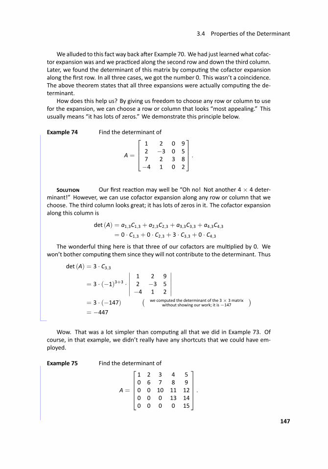
3.4 Proper es of the Determinant
We alluded to this fact way back a er Example 70. We had just learnedwhat cofac-tor expansion was and we prac ced along the second row and down the third column.Later, we found the determinant of this matrix by compu ng the cofactor expansionalong the first row. In all three cases, we got the number 0. This wasn’t a coincidence.The above theorem states that all three expansions were actually compu ng the de-terminant.
How does this help us? By giving us freedom to choose any row or column to usefor the expansion, we can choose a row or column that looks “most appealing.” Thisusually means “it has lots of zeros.” We demonstrate this principle below.
.. Example 74 Find the determinant of
A =
1 2 0 92 −3 0 57 2 3 8−4 1 0 2
.
S Our first reac on may well be “Oh no! Not another 4 × 4 deter-minant!” However, we can use cofactor expansion along any row or column that wechoose. The third column looks great; it has lots of zeros in it. The cofactor expansionalong this column is
det (A) = a1,3C1,3 + a2,3C2,3 + a3,3C3,3 + a4,3C4,3= 0 · C1,3 + 0 · C2,3 + 3 · C3,3 + 0 · C4,3
The wonderful thing here is that three of our cofactors are mul plied by 0. Wewon’t bother compu ng them since they will not contribute to the determinant. Thus
det (A) = 3 · C3,3
= 3 · (−1)3+3 ·
∣∣∣∣∣∣1 2 92 −3 5−4 1 2
∣∣∣∣∣∣= 3 · (−147)
( we computed the determinant of the 3 × 3 matrixwithout showing our work; it is−147
)= −447
..
Wow. That was a lot simpler than compu ng all that we did in Example 73. Ofcourse, in that example, we didn’t really have any shortcuts that we could have em-ployed.
.. Example 75 ..Find the determinant of
A =
1 2 3 4 50 6 7 8 90 0 10 11 120 0 0 13 140 0 0 0 15
.
147
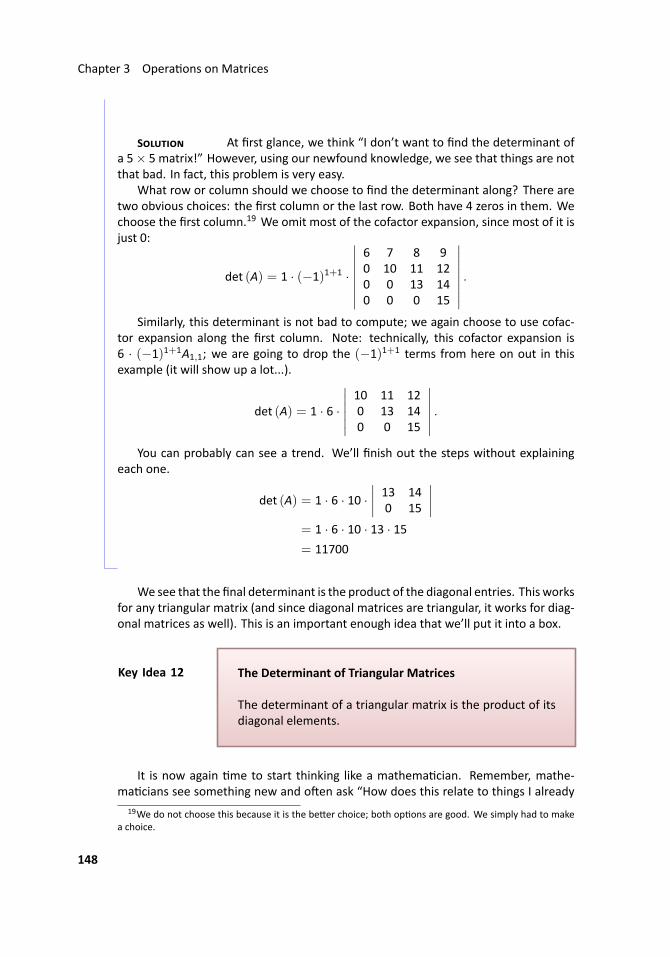
Chapter 3 Opera ons on Matrices
S At first glance, we think “I don’t want to find the determinant ofa 5× 5 matrix!” However, using our newfound knowledge, we see that things are notthat bad. In fact, this problem is very easy.
What row or column should we choose to find the determinant along? There aretwo obvious choices: the first column or the last row. Both have 4 zeros in them. Wechoose the first column.19 We omit most of the cofactor expansion, since most of it isjust 0:
det (A) = 1 · (−1)1+1 ·
∣∣∣∣∣∣∣∣6 7 8 90 10 11 120 0 13 140 0 0 15
∣∣∣∣∣∣∣∣ .Similarly, this determinant is not bad to compute; we again choose to use cofac-
tor expansion along the first column. Note: technically, this cofactor expansion is6 · (−1)1+1A1,1; we are going to drop the (−1)1+1 terms from here on out in thisexample (it will show up a lot...).
det (A) = 1 · 6 ·
∣∣∣∣∣∣10 11 120 13 140 0 15
∣∣∣∣∣∣ .You can probably can see a trend. We’ll finish out the steps without explaining
each one.
det (A) = 1 · 6 · 10 ·∣∣∣∣ 13 14
0 15
∣∣∣∣= 1 · 6 · 10 · 13 · 15= 11700
...
We see that the final determinant is the product of the diagonal entries. This worksfor any triangular matrix (and since diagonal matrices are triangular, it works for diag-onal matrices as well). This is an important enough idea that we’ll put it into a box.
..Key Idea 12
.
.The Determinant of Triangular Matrices
The determinant of a triangular matrix is the product of itsdiagonal elements.
It is now again me to start thinking like a mathema cian. Remember, mathe-ma cians see something new and o en ask “How does this relate to things I already
19We do not choose this because it is the be er choice; both op ons are good. We simply had to makea choice.
148
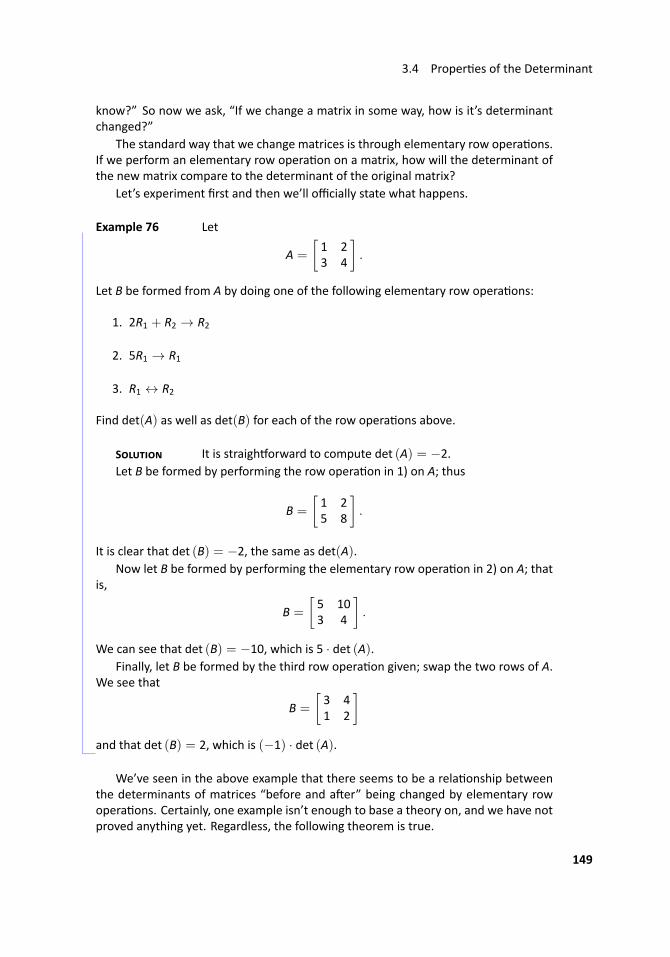
3.4 Proper es of the Determinant
know?” So now we ask, “If we change a matrix in some way, how is it’s determinantchanged?”
The standard way that we change matrices is through elementary row opera ons.If we perform an elementary row opera on on a matrix, how will the determinant ofthe new matrix compare to the determinant of the original matrix?
Let’s experiment first and then we’ll officially state what happens.
.. Example 76 Let
A =
[1 23 4
].
Let B be formed from A by doing one of the following elementary row opera ons:
1. 2R1 + R2 → R2
2. 5R1 → R1
3. R1 ↔ R2
Find det(A) as well as det(B) for each of the row opera ons above.
S It is straigh orward to compute det (A) = −2.Let B be formed by performing the row opera on in 1) on A; thus
B =
[1 25 8
].
It is clear that det (B) = −2, the same as det(A).Now let B be formed by performing the elementary row opera on in 2) on A; that
is,
B =
[5 103 4
].
We can see that det (B) = −10, which is 5 · det (A).Finally, let B be formed by the third row opera on given; swap the two rows of A.
We see that
B =
[3 41 2
]and that det (B) = 2, which is (−1) · det (A). ..
We’ve seen in the above example that there seems to be a rela onship betweenthe determinants of matrices “before and a er” being changed by elementary rowopera ons. Certainly, one example isn’t enough to base a theory on, and we have notproved anything yet. Regardless, the following theorem is true.
149
Chapter 3 Opera ons on Matrices
..Theorem 15
.
.The Determinant and Elementary Row Opera ons
Let A be an n× nmatrix and let B be formed by performingone elementary row opera on on A.
1. If B is formed from A by adding a scalar mul ple ofone row to another, then det (B) = det (A).
2. If B is formed from A by mul plying one row of A by ascalar k, then det (B) = k · det (A).
3. If B is formed from A by interchanging two rows of A,then det (B) = −det (A).
Let’s put this theorem to use in an example.
.. Example 77 Let
A =
1 2 10 1 11 1 1
.
Compute det(A), then find the determinants of the following matrices by inspec onusing Theorem 15.
B =
1 1 11 2 10 1 1
C =
1 2 10 1 17 7 7
D =
1 −1 −20 1 11 1 1
S Compu ng det(A) by cofactor expansion down the first column oralong the second row seems like the best choice, u lizing the one zero in the matrix.We can quickly confirm that det (A) = 1.
To compute det(B), no ce that the rows of Awere rearranged to form B. There aredifferent ways to describe what happened; saying R1 ↔ R2 was followed by R1 ↔ R3produces B from A. Since there were two row swaps, det (B) = (−1)(−1)det (A) =det (A) = 1.
No ce that C is formed from A by mul plying the third row by 7. Thus det (C) =7 · det (A) = 7.
It takes a li le thought, butwe can formD fromAby the opera on−3R2+R1 → R1.This type of elementary row opera on does not change determinants, so det (D) =det (A). ..
150
3.4 Proper es of the Determinant
Let’s con nue to think like mathema cians; mathema cians tend to remember“problems” they’ve encountered in the past,20 and when they learn something new,in the backs of their minds they try to apply their new knowledge to solve their oldproblem.
What “problem” did we recently uncover? We stated in the last chapter that evencomputers could not compute the determinant of large matrices with cofactor expan-sion. How then can we compute the determinant of large matrices?
We just learned two interes ng and useful facts about matrix determinants. First,the determinant of a triangular matrix is easy to compute: just mul ply the diagonalelements. Secondly, we know how elementary row opera ons affect the determinant.Put these two ideas together: given any squarematrix, we can use elementary row op-era ons to put the matrix in triangular form,21 find the determinant of the newmatrix(which is easy), and then adjust that number by recalling what elementary opera onswe performed. Let’s prac ce this.
.. Example 78 ..Find the determinant of A by first pu ng A into a triangular form,where
A =
2 4 −2−1 −2 53 2 1
.
S In pu ng A into a triangular form, we need not worry about get-ng leading 1s, but it does tend to make our life easier as we work out a problem by
hand. So let’s scale the first row by 1/2:
12R1 → R1
1 2 −1−1 −2 53 2 1
.
Now let’s get 0s below this leading 1:
R1 + R2 → R2
−3R1 + R3 → R3
1 2 −10 0 40 −4 4
.
We can finish in one step; by interchanging rows 2 and 3 we’ll have our matrix intriangular form.
R2 ↔ R3
1 2 −10 −4 40 0 4
.
Let’s name this last matrix B. The determinant of B is easy to compute as it istriangular; det (B) = −16. We can use this to find det(A).
Recall the steps we used to transform A into B. They are:
20which is why mathema cians rarely smile: they are remembering their problems21or echelon form
151
Chapter 3 Opera ons on Matrices
12R1 → R1
R1 + R2 → R2−3R1 + R3 → R3
R2 ↔ R3
The first opera on mul plied a row of A by 12 . This means that the resul ng matrix
had a determinant that was 12 the determinant of A.
The next two opera ons did not affect the determinant at all. The last opera on,the row swap, changed the sign. Combining these effects, we know that
−16 = det (B) = (−1)12det (A) .
Solving for det (A) we have that det (A) = 32. ...
In prac ce, we don’t need to keep track of opera ons where we add mul plesof one row to another; they simply do not affect the determinant. Also, in prac ce,these steps are carried out by a computer, and computers don’t care about leading 1s.Therefore, row scaling opera ons are rarely used. The only things to keep track of arerow swaps, and even then all we care about are the number of row swaps. An oddnumber of row swaps means that the original determinant has the opposite sign ofthe triangular form matrix; an even number of row swaps means they have the samedeterminant.
Let’s prac ce this again.
.. Example 79 The matrix B was formed from A using the following elementaryrow opera ons, though not necessarily in this order. Find det(A).
B =
1 2 30 4 50 0 6
2R1 → R113R3 → R3R1 ↔ R26R1 + R2 → R2
S It is easy to compute det (B) = 24. In looking at our list of elemen-tary row opera ons, we see that only the first three have an effect on the determinant.Therefore
24 = det (B) = 2 · 13· (−1) · det (A)
and hencedet (A) = −36...
In the previous example, we may have been tempted to “rebuild” A using the ele-mentary row opera ons and then compu ng the determinant. This can be done, butin general it is a bad idea; it takes too much work and it is too easy to make a mistake.
Let’s think somemore like a mathema cian. How does the determinant work withother matrix opera ons that we know? Specifically, how does the determinant in-teract with matrix addi on, scalar mul plica on, matrix mul plica on, the transpose
152
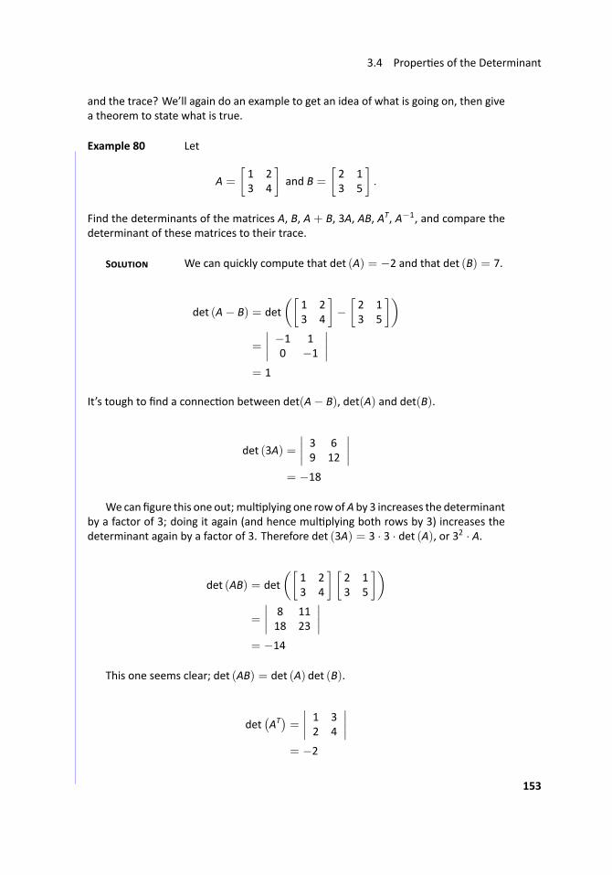
3.4 Proper es of the Determinant
and the trace? We’ll again do an example to get an idea of what is going on, then givea theorem to state what is true.
.. Example 80 ..Let
A =
[1 23 4
]and B =
[2 13 5
].
Find the determinants of the matrices A, B, A + B, 3A, AB, AT, A−1, and compare thedeterminant of these matrices to their trace.
S We can quickly compute that det (A) = −2 and that det (B) = 7.
det (A− B) = det([
1 23 4
]−
[2 13 5
])=
∣∣∣∣ −1 10 −1
∣∣∣∣= 1
It’s tough to find a connec on between det(A− B), det(A) and det(B).
det (3A) =
∣∣∣∣ 3 69 12
∣∣∣∣= −18
We can figure this one out; mul plying one rowofA by 3 increases the determinantby a factor of 3; doing it again (and hence mul plying both rows by 3) increases thedeterminant again by a factor of 3. Therefore det (3A) = 3 · 3 · det (A), or 32 · A.
det (AB) = det([
1 23 4
] [2 13 5
])=
∣∣∣∣ 8 1118 23
∣∣∣∣= −14
This one seems clear; det (AB) = det (A) det (B).
det(AT) = ∣∣∣∣ 1 3
2 4
∣∣∣∣= −2
153
Chapter 3 Opera ons on Matrices
Obviously det(AT)= det (A); is this always going to be the case? If we think about
it, we can see that the cofactor expansion along the first row of Awill give us the sameresult as the cofactor expansion along the first column of AT.22
det(A−1) = ∣∣∣∣ −2 1
3/2 −1/2
∣∣∣∣= 1− 3/2
= −1/2
It seems as though
det(A−1) = 1
det (A).
We end by remarking that there seems to be no connec on whatsoever betweenthe trace of a matrix and its determinant. We leave it to the reader to compute thetrace for some of the above matrices and confirm this statement....
We now state a theorem which will confirm our conjectures from the previousexample.
..Theorem 16
.
.Determinant Proper es
Let A and B be n × n matrices and let k be a scalar. Thefollowing are true:
1. det (kA) = kn · det (A)
2. det(AT)= det (A)
3. det (AB) = det (A) det (B)
4. If A is inver ble, then
det(A−1) = 1
det (A).
5. A matrix A is inver ble if and only if det (A) = 0.
This last statement of the above theorem is significant: what happens if det (A) =0? It seems that det
(A−1
)=“1/0”, which is undefined. There actually isn’t a problem
here; it turns out that if det (A) = 0, then A is not inver ble (hence part 5 of Theorem16). This allows us to add on to our Inver ble Matrix Theorem.
22This can be a bit tricky to think out in your head. Try it with a 3×3 matrix A and see how it works. Allthe 2×2 submatrices that are created in AT are the transpose of those found in A; this doesn’t ma er sinceit is easy to see that the determinant isn’t affected by the transpose in a 2× 2 matrix.
154
3.4 Proper es of the Determinant
..Theorem 17
.
.Inver ble Matrix Theorem
LetA be an n×nmatrix. The following statements are equiv-alent.
(a) A is inver ble.
(g) det (A) = 0.
This new addi on to the Inver ble Matrix Theorem is very useful; we’ll refer backto it in Chapter 4 when we discuss eigenvalues.
We end this sec on with a shortcut for compu ng the determinants of 3× 3 ma-trices. Consider the matrix A: 1 2 3
4 5 67 8 9
.
We can compute its determinant using cofactor expansion as we did in Example 71.Once one becomes proficient at this method, compu ng the determinant of a 3 × 3isn’t all that hard. A method many find easier, though, starts with rewri ng the matrixwithout the brackets, and repea ng the first and second columns at the end as shownbelow.
1 2 3 1 24 5 6 4 57 8 9 7 8
In this 3 × 5 array of numbers, there are 3 full “upper le to lower right” diagonals,and 3 full “upper right to lower le ” diagonals, as shown below with the arrows.
..1 2 3 1 24 5 6 4 57 8 9 7 8
.
45
.
84
.
96
.
105
.
48
.
72
The numbers that appear at the ends of each of the arrows are computed by mul-plying the numbers found along the arrows. For instance, the 105 comes from mul-plying 3 · 5 · 7 = 105. The determinant is found by adding the numbers on the right,
and subtrac ng the sum of the numbers on the le . That is,
det (A) = (45+ 84+ 96)− (105+ 48+ 72) = 0.
To help remind ourselves of this shortcut, we’ll make it into a Key Idea.
155
Chapter 3 Opera ons on Matrices
..Key Idea 13
.
.3× 3 Determinant Shortcut
Let A be a 3 × 3 matrix. Create a 3 × 5 array by repea ngthe first 2 columns and consider the products of the 3 “righthand” diagonals and 3 “le hand” diagonals as shown pre-viously. Then
det (A) = “(the sum of the right hand numbers)
− (the sum of the le hand numbers)”.
We’ll prac ce once more in the context of an example.
.. Example 81 Find the determinant of A using the previously described shortcut,where
A =
1 3 9−2 3 4−5 7 2
.
S Rewri ng the first 2 columns, drawing the proper diagonals, andmul plying, we get:
..1 3 9 1 3−2 3 4 −2 3−5 7 2 −5 7
.
6
.
−60
.
−126
.
−135
.
28
.
−12
Summing the numbers on the right and subtrac ng the sum of the numbers on thele , we get
det (A) = (6− 60− 126)− (−135+ 28− 12) = −61.
..In the next sec on we’ll see how the determinant can be used to solve systems of
linear equa ons.
Exercises 3.4In Exercises 1 – 14, find the determinantof the given matrix using cofactor expansionalong any row or column you choose.
1.
1 2 3−5 0 34 0 6
2.
−4 4 −40 0 −3−2 −2 −1
3.
−4 1 10 0 0−1 −2 −5
156
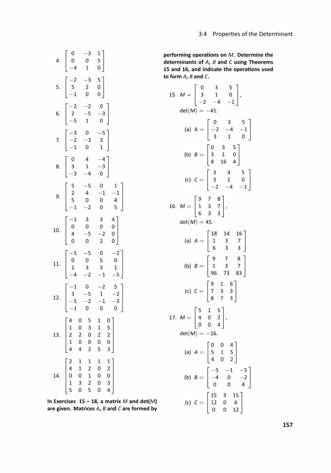
3.4 Proper es of the Determinant
4.
0 −3 10 0 5−4 1 0
5.
−2 −3 55 2 0−1 0 0
6.
−2 −2 02 −5 −3−5 1 0
7.
−3 0 −5−2 −3 3−1 0 1
8.
0 4 −43 1 −3−3 −4 0
9.
5 −5 0 12 4 −1 −15 0 0 4−1 −2 0 5
10.
−1 3 3 40 0 0 04 −5 −2 00 0 2 0
11.
−5 −5 0 −20 0 5 01 3 3 1−4 −2 −1 −5
12.
−1 0 −2 53 −5 1 −2−5 −2 −1 −3−1 0 0 0
13.
4 0 5 1 01 0 3 1 52 2 0 2 21 0 0 0 04 4 2 5 3
14.
2 1 1 1 14 1 2 0 20 0 1 0 01 3 2 0 35 0 5 0 4
In Exercises 15 – 18, a matrix M and det(M)are given. Matrices A, B and C are formed by
performing opera ons on M. Determine thedeterminants of A, B and C using Theorems15 and 16, and indicate the opera ons usedto form A, B and C.
15. M =
0 3 53 1 0−2 −4 −1
,det(M) = −41.
(a) A =
0 3 5−2 −4 −13 1 0
(b) B =
0 3 53 1 08 16 4
(c) C =
3 4 53 1 0−2 −4 −1
16. M =
9 7 81 3 76 3 3
,det(M) = 45.
(a) A =
18 14 161 3 76 3 3
(b) B =
9 7 81 3 796 73 83
(c) C =
9 1 67 3 38 7 3
17. M =
5 1 54 0 20 0 4
,det(M) = −16.
(a) A =
0 0 45 1 54 0 2
(b) B =
−5 −1 −5−4 0 −20 0 4
(c) C =
15 3 1512 0 60 0 12
157
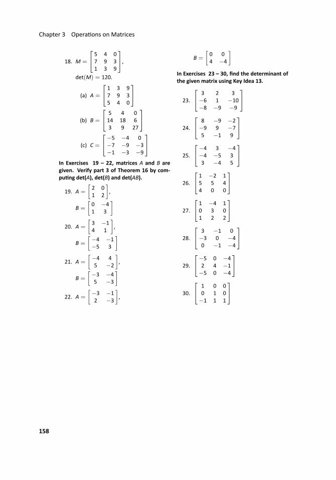
Chapter 3 Opera ons on Matrices
18. M =
5 4 07 9 31 3 9
,det(M) = 120.
(a) A =
1 3 97 9 35 4 0
(b) B =
5 4 014 18 63 9 27
(c) C =
−5 −4 0−7 −9 −3−1 −3 −9
In Exercises 19 – 22, matrices A and B aregiven. Verify part 3 of Theorem 16 by com-pu ng det(A), det(B) and det(AB).
19. A =
[2 01 2
],
B =
[0 −41 3
]20. A =
[3 −14 1
],
B =
[−4 −1−5 3
]21. A =
[−4 45 −2
],
B =
[−3 −45 −3
]22. A =
[−3 −12 −3
],
B =
[0 04 −4
]In Exercises 23 – 30, find the determinant ofthe given matrix using Key Idea 13.
23.
3 2 3−6 1 −10−8 −9 −9
24.
8 −9 −2−9 9 −75 −1 9
25.
−4 3 −4−4 −5 33 −4 5
26.
1 −2 15 5 44 0 0
27.
1 −4 10 3 01 2 2
28.
3 −1 0−3 0 −40 −1 −4
29.
−5 0 −42 4 −1−5 0 −4
30.
1 0 00 1 0−1 1 1
158
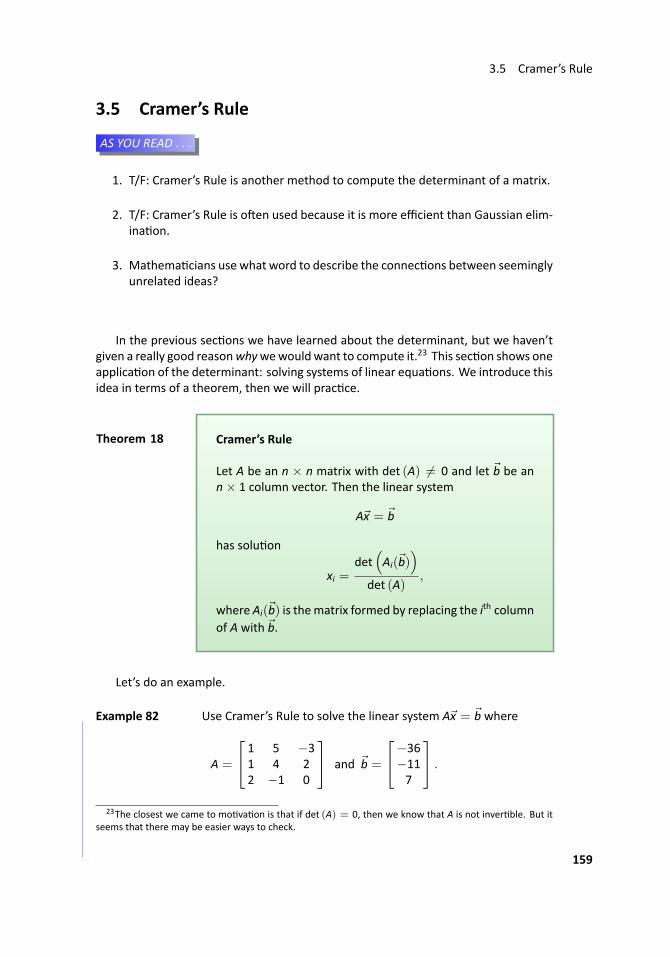
3.5 Cramer’s Rule
3.5 Cramer’s Rule
...AS YOU READ . . .
1. T/F: Cramer’s Rule is another method to compute the determinant of a matrix.
2. T/F: Cramer’s Rule is o en used because it is more efficient than Gaussian elim-ina on.
3. Mathema cians use what word to describe the connec ons between seeminglyunrelated ideas?
In the previous sec ons we have learned about the determinant, but we haven’tgiven a really good reasonwhywewouldwant to compute it.23 This sec on shows oneapplica on of the determinant: solving systems of linear equa ons. We introduce thisidea in terms of a theorem, then we will prac ce.
..Theorem 18
.
.Cramer’s Rule
Let A be an n × n matrix with det (A) = 0 and let b be ann× 1 column vector. Then the linear system
Ax = b
has solu on
xi =det
(Ai(b)
)det (A)
,
where Ai(b) is thematrix formed by replacing the ith columnof A with b.
Let’s do an example.
.. Example 82 ..Use Cramer’s Rule to solve the linear system Ax = b where
A =
1 5 −31 4 22 −1 0
and b =
−36−117
.
23The closest we came to mo va on is that if det (A) = 0, then we know that A is not inver ble. But itseems that there may be easier ways to check.
159
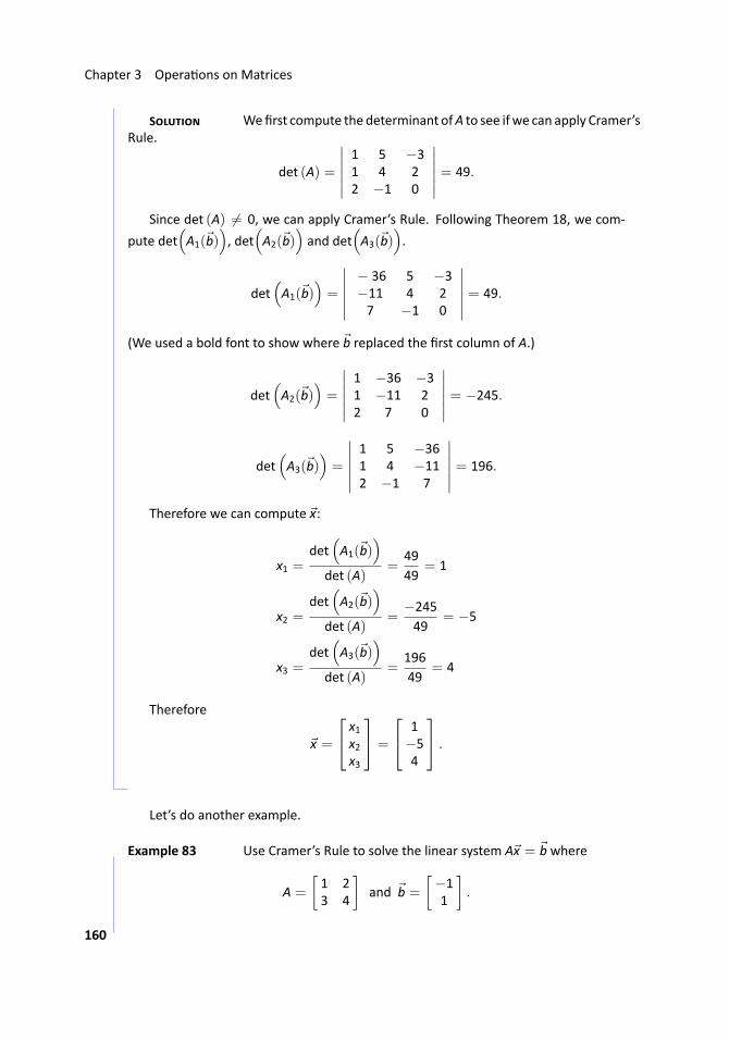
Chapter 3 Opera ons on Matrices
S Wefirst compute thedeterminant ofA to see ifwe can apply Cramer’sRule.
det (A) =
∣∣∣∣∣∣1 5 −31 4 22 −1 0
∣∣∣∣∣∣ = 49.
Since det (A) = 0, we can apply Cramer’s Rule. Following Theorem 18, we com-
pute det(A1(b)
), det
(A2(b)
)and det
(A3(b)
).
det(A1(b)
)=
∣∣∣∣∣∣− 36 5 −3−11 4 27 −1 0
∣∣∣∣∣∣ = 49.
(We used a bold font to show where b replaced the first column of A.)
det(A2(b)
)=
∣∣∣∣∣∣1 −36 −31 −11 22 7 0
∣∣∣∣∣∣ = −245.
det(A3(b)
)=
∣∣∣∣∣∣1 5 −361 4 −112 −1 7
∣∣∣∣∣∣ = 196.
Therefore we can compute x:
x1 =det
(A1(b)
)det (A)
=4949
= 1
x2 =det
(A2(b)
)det (A)
=−24549
= −5
x3 =det
(A3(b)
)det (A)
=19649
= 4
Therefore
x =
x1x2x3
=
1−54
.
...
Let’s do another example.
.. Example 83 ..Use Cramer’s Rule to solve the linear system Ax = b where
A =
[1 23 4
]and b =
[−11
].
160
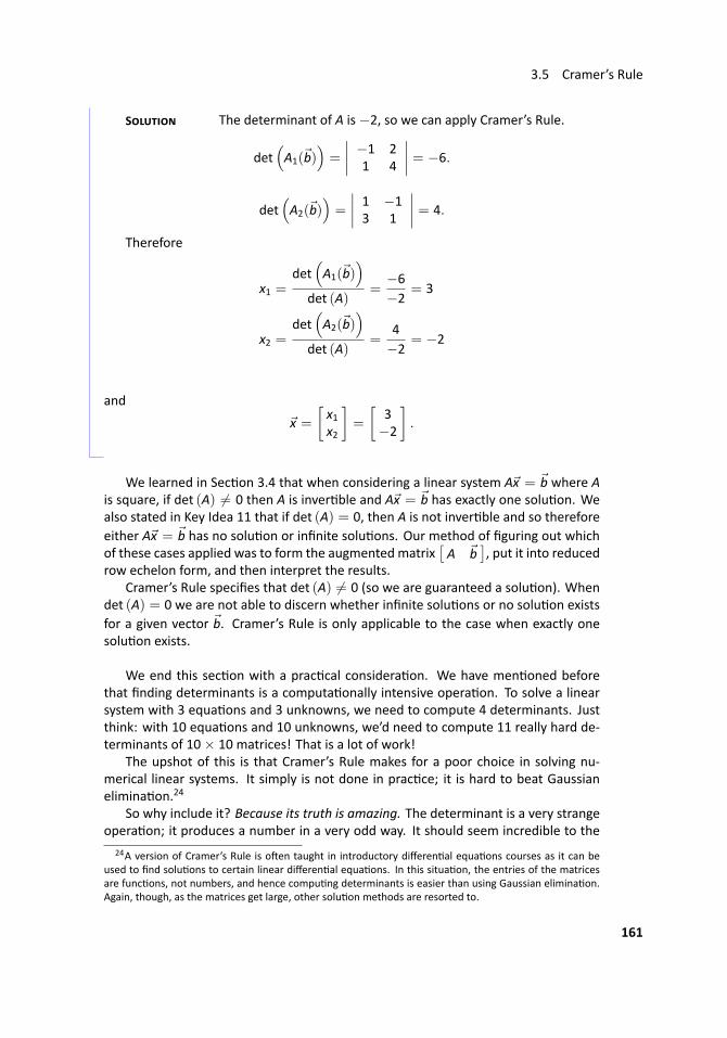
3.5 Cramer’s Rule
S The determinant of A is−2, so we can apply Cramer’s Rule.
det(A1(b)
)=
∣∣∣∣ −1 21 4
∣∣∣∣ = −6.
det(A2(b)
)=
∣∣∣∣ 1 −13 1
∣∣∣∣ = 4.
Therefore
x1 =det
(A1(b)
)det (A)
=−6−2
= 3
x2 =det
(A2(b)
)det (A)
=4−2
= −2
and
x =
[x1x2
]=
[3−2
].
...
We learned in Sec on 3.4 that when considering a linear system Ax = b where Ais square, if det (A) = 0 then A is inver ble and Ax = b has exactly one solu on. Wealso stated in Key Idea 11 that if det (A) = 0, then A is not inver ble and so thereforeeither Ax = b has no solu on or infinite solu ons. Our method of figuring out whichof these cases applied was to form the augmented matrix
[A b
], put it into reduced
row echelon form, and then interpret the results.Cramer’s Rule specifies that det (A) = 0 (so we are guaranteed a solu on). When
det (A) = 0 we are not able to discern whether infinite solu ons or no solu on existsfor a given vector b. Cramer’s Rule is only applicable to the case when exactly onesolu on exists.
We end this sec on with a prac cal considera on. We have men oned beforethat finding determinants is a computa onally intensive opera on. To solve a linearsystem with 3 equa ons and 3 unknowns, we need to compute 4 determinants. Justthink: with 10 equa ons and 10 unknowns, we’d need to compute 11 really hard de-terminants of 10× 10 matrices! That is a lot of work!
The upshot of this is that Cramer’s Rule makes for a poor choice in solving nu-merical linear systems. It simply is not done in prac ce; it is hard to beat Gaussianelimina on.24
So why include it? Because its truth is amazing. The determinant is a very strangeopera on; it produces a number in a very odd way. It should seem incredible to the
24A version of Cramer’s Rule is o en taught in introductory differen al equa ons courses as it can beused to find solu ons to certain linear differen al equa ons. In this situa on, the entries of the matricesare func ons, not numbers, and hence compu ng determinants is easier than using Gaussian elimina on.Again, though, as the matrices get large, other solu on methods are resorted to.
161
Chapter 3 Opera ons on Matrices
reader that by manipula ng determinants in a par cular way, we can solve linear sys-tems.
In the next chapter we’ll see another use for the determinant. Meanwhile, try todevelop a deeper apprecia on ofmath: odd, complicated things that seem completelyunrelated o en are intricately ed together. Mathema cians see these connec onsand describe them as “beau ful.”
Exercises 3.5In Exercises 1 – 12,matricesA and b are given.
(a) Give det(A) and det(Ai) for all i.
(b) Use Cramer’s Rule to solve Ax = b. IfCramer’s Rule cannot be used to findthe solu on, then statewhether or nota solu on exists.
1. A =
[7 −7−7 9
], b =
[28−26
]2. A =
[9 5−4 −7
], b =
[−4520
]3. A =
[−8 1610 −20
], b =
[−4860
]4. A =
[0 −69 −10
], b =
[6
−17
]5. A =
[2 10−1 3
], b =
[4219
]6. A =
[7 14−2 −4
], b =
[−14
]
7. A =
3 0 −35 4 45 5 −4
, b =
24031
8. A =
4 9 3−5 −2 −13−1 10 −13
,
b =
−28357
9. A =
4 −4 05 1 −13 −1 2
, b =
16228
10. A =
1 0 −104 −3 −10−9 6 −2
,b =
−40−94132
11. A =
7 −4 25−2 1 −79 −7 34
,b =
−1−35
12. A =
−6 −7 −75 4 15 4 8
,b =
58−35−49
162
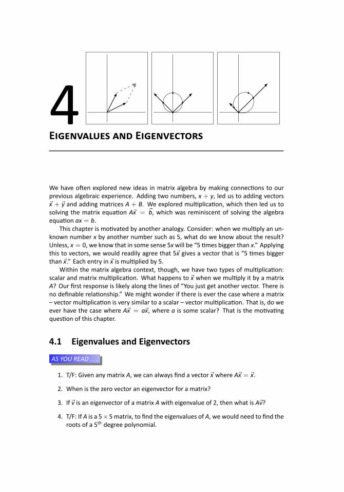
4 .
E E
We have o en explored new ideas in matrix algebra by making connec ons to ourprevious algebraic experience. Adding two numbers, x + y, led us to adding vectorsx + y and adding matrices A + B. We explored mul plica on, which then led us tosolving the matrix equa on Ax = b, which was reminiscent of solving the algebraequa on ax = b.
This chapter is mo vated by another analogy. Consider: when we mul ply an un-known number x by another number such as 5, what do we know about the result?Unless, x = 0, we know that in some sense 5xwill be “5 mes bigger than x.” Applyingthis to vectors, we would readily agree that 5x gives a vector that is “5 mes biggerthan x.” Each entry in x is mul plied by 5.
Within the matrix algebra context, though, we have two types of mul plica on:scalar and matrix mul plica on. What happens to x when we mul ply it by a matrixA? Our first response is likely along the lines of “You just get another vector. There isno definable rela onship.” We might wonder if there is ever the case where a matrix– vector mul plica on is very similar to a scalar – vector mul plica on. That is, do weever have the case where Ax = ax, where a is some scalar? That is the mo va ngques on of this chapter.
4.1 Eigenvalues and Eigenvectors
...AS YOU READ . . .
1. T/F: Given any matrix A, we can always find a vector x where Ax = x.
2. When is the zero vector an eigenvector for a matrix?
3. If v is an eigenvector of a matrix A with eigenvalue of 2, then what is Av?
4. T/F: If A is a 5×5matrix, to find the eigenvalues of A, we would need to find theroots of a 5th degree polynomial.
Chapter 4 Eigenvalues and Eigenvectors
We start by considering the matrix A and vector x as given below.1
A =
[1 42 3
]x =
[11
]Mul plying Ax gives:
Ax =
[1 42 3
] [11
]=
[55
]= 5
[11
]!
Wow! It looks like mul plying Ax is the same as 5x! This makes us wonder lotsof things: Is this the only case in the world where something like this happens?2 Is Asomehow a special matrix, and Ax = 5x for any vector x we pick?3 Or maybe x was aspecial vector, and noma er what 2×2matrix Awe picked, wewould have Ax = 5x.4
A more likely explana on is this: given the matrix A, the number 5 and the vectorx formed a special pair that happened to work together in a nice way. It is then naturalto wonder if other “special” pairs exist. For instance, could we find a vector x whereAx = 3x?
This equa on is hard to solve at first; we are not used to matrix equa ons wherex appears on both sides of “=.” Therefore we put off solving this for just a moment tostate a defini on and make a few comments.
..Defini on 27
.
.Eigenvalues and Eigenvectors
Let A be an n × n matrix, x a nonzero n × 1 column vectorand λ a scalar. If
Ax = λx,
then x is an eigenvector of A and λ is an eigenvalue of A.
The word “eigen” is German for “proper” or “characteris c.” Therefore, an eigen-vector of A is a “characteris c vector of A.” This vector tells us something about A.
Why do we use the Greek le er λ (lambda)? It is pure tradi on. Above, we used ato represent the unknown scalar, since we are used to that nota on. We now switchto λ because that is how everyone else does it.5 Don’t get hung up on this; λ is just anumber.
1Recall this matrix and vector were used in Example 40 on page 75.2Probably not.3Probably not.4See footnote 2.5An example of mathema cal peer pressure.
164
4.1 Eigenvalues and Eigenvectors
Note that our defini on requires that A be a square matrix. If A isn’t square thenAx and λx will have different sizes, and so they cannot be equal. Also note that x mustbe nonzero. Why? What if x = 0? Then no ma er what λ is, Ax = λx. This wouldthen imply that every number is an eigenvalue; if every number is an eigenvalue, thenwe wouldn’t need a defini on for it.6 Therefore we specify that x = 0.
Our last comment before trying to find eigenvalues and eigenvectors for given ma-trices deals with “why we care.” Did we stumble upon a mathema cal curiosity, ordoes this somehow help us build be er bridges, heal the sick, send astronauts intoorbit, design op cal equipment, and understand quantummechanics? The answer, ofcourse, is “Yes.”7 This is a wonderful topic in and of itself: we need no external applica-on to appreciate its worth. At the same me, it has many, many applica ons to “the
real world.” A simple Internet seach on “applica ons of eigenvalues”with confirm this.Back to our math. Given a square matrix A, we want to find a nonzero vector x
and a scalar λ such that Ax = λx. We will solve this using the skills we developed inChapter 2.
Ax = λx original equa on
Ax − λx = 0 subtract λx from both sides
(A− λI)x = 0 factor out x
Think about this last factoriza on. We are likely tempted to say
Ax − λx = (A− λ)x,
but this really doesn’t make sense. A er all, what does “a matrix minus a number”mean? We need the iden ty matrix in order for this to be logical.
Let us now think about the equa on (A− λI)x = 0. While it looks complicated, itreally is just matrix equa on of the type we solved in Sec on 2.4. We are just tryingto solve Bx = 0, where B = (A− λI).
We know from our previous work that this type of equa on8 always has a solu on,namely, x = 0. However, we want x to be an eigenvector and, by the defini on,eigenvectors cannot be 0.
This means that we want solu ons to (A − λI)x = 0 other than x = 0. Recallthat Theorem 8 says that if the matrix (A− λI) is inver ble, then the only solu on to(A− λI)x = 0 is x = 0. Therefore, in order to have other solu ons, we need (A− λI)to not be inver ble.
Finally, recall from Theorem 16 that noninver ble matrices all have a determi-nant of 0. Therefore, if we want to find eigenvalues λ and eigenvectors x, we needdet (A− λI) = 0.
Let’s start our prac ce of this theory by finding λ such that det (A− λI) = 0; thatis, let’s find the eigenvalues of a matrix.
6Recall footnote 17 on page 107.7Except for the “understand quantum mechanics” part. Nobody truly understands that stuff; they just
probably understand it.8Recall this is a homogeneous system of equa ons.
165
Chapter 4 Eigenvalues and Eigenvectors
.. Example 84 Find the eigenvalues ofA, that is, findλ such that det (A− λI) = 0,where
A =
[1 42 3
].
S (Note that this is the matrix we used at the beginning of this sec-on.) First, we write out what A− λI is:
A− λI =[1 42 3
]− λ
[1 00 1
]=
[1 42 3
]−[λ 00 λ
]=
[1− λ 42 3− λ
]Therefore,
det (A− λI) =
∣∣∣∣ 1− λ 42 3− λ
∣∣∣∣= (1− λ)(3− λ)− 8
= λ2 − 4λ− 5
Since we want det (A− λI) = 0, we want λ2 − 4λ − 5 = 0. This is a simplequadra c equa on that is easy to factor:
λ2 − 4λ− 5 = 0
(λ− 5)(λ+ 1) = 0
λ = −1, 5
According to our above work, det (A− λI) = 0 when λ = −1, 5. Thus, the eigen-values of A are−1 and 5. ..
Earlier, when looking at the same matrix as used in our example, we wondered ifwe could find a vector x such that Ax = 3x. According to this example, the answer is“No.” With this matrix A, the only values of λ that work are−1 and 5.
Let’s restate the above in a different way: It is pointless to try to find x whereAx = 3x, for there is no such x. There are only 2 equa ons of this form that have asolu on, namely
Ax = −x and Ax = 5x.
As we introduced this sec on, we gave a vector x such that Ax = 5x. Is this theonly one? Let’s find out while calling our work an example; this will amount to findingthe eigenvectors of A that correspond to the eigenvector of 5.
166
4.1 Eigenvalues and Eigenvectors
.. Example 85 Find x such that Ax = 5x, where
A =
[1 42 3
].
S Recall that our algebra from before showed that if
Ax = λx then (A− λI)x = 0.
Therefore, we need to solve the equa on (A− λI)x = 0 for x when λ = 5.
A− 5I =[1 42 3
]− 5
[1 00 1
]=
[−4 42 −2
]To solve (A−5I)x = 0, we form the augmentedmatrix and put it into reduced row
echelon form: [−4 4 02 −2 0
]−→rref
[1 −1 00 0 0
].
Thus
x1 = x2x2 is free
and
x =
[x1x2
]= x2
[11
].
We have infinite solu ons to the equa on Ax = 5x; any nonzero scalar mul ple of the
vector[11
]is a solu on. We can do a few examples to confirm this:
[1 42 3
] [22
]=
[1010
]= 5
[22
];
[1 42 3
] [77
]=
[3535
]= 5
[77
];
[1 42 3
] [−3−3
]=
[−15−15
]= 5
[−3−3
].
..Our method of finding the eigenvalues of a matrix A boils down to determining
which values ofλ give thematrix (A−λI) adeterminant of 0. In compu ngdet (A− λI),we get a polynomial in λ whose roots are the eigenvalues of A. This polynomial is im-portant and so it gets its own name.
167
Chapter 4 Eigenvalues and Eigenvectors
..Defini on 28
.
.Characteris c Polynomial
Let A be an n× nmatrix. The characteris c polynomial of Ais the nth degree polynomial p(λ) = det (A− λI).
Our defini on just stateswhat the characteris c polynomial is. We know from ourwork so far why we care: the roots of the characteris c polynomial of an n× nmatrixA are the eigenvalues of A.
In Examples 84 and 85, we found eigenvalues and eigenvectors, respec vely, ofa given matrix. That is, given a matrix A, we found values λ and vectors x such thatAx = λx. The steps that follow outline the general procedure for finding eigenvaluesand eigenvectors; we’ll follow this up with some examples.
..Key Idea 14
.
.Finding Eigenvalues and Eigenvectors
Let A be an n× nmatrix.
1. To find the eigenvalues of A, compute p(λ), the char-acteris c polynomial of A, set it equal to 0, then solvefor λ.
2. To find the eigenvectors of A, for each eigenvaluesolve the homogeneous system (A− λI)x = 0.
.. Example 86 ..Find the eigenvalues of A, and for each eigenvalue, find an eigen-vector where
A =
[−3 153 9
].
S To find the eigenvalues, we must compute det (A− λI) and set itequal to 0.
det (A− λI) =
∣∣∣∣ −3− λ 153 9− λ
∣∣∣∣= (−3− λ)(9− λ)− 45
= λ2 − 6λ− 27− 45
= λ2 − 6λ− 72
= (λ− 12)(λ+ 6)
Therefore, det (A− λI) = 0 when λ = −6 and 12; these are our eigenvalues. (We
168
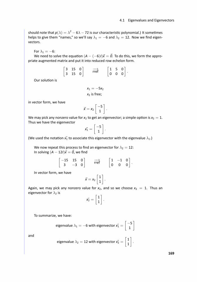
4.1 Eigenvalues and Eigenvectors
should note that p(λ) = λ2 − 6λ− 72 is our characteris c polynomial.) It some meshelps to give them “names,” so we’ll say λ1 = −6 and λ2 = 12. Now we find eigen-vectors.
For λ1 = −6:We need to solve the equa on (A − (−6)I)x = 0. To do this, we form the appro-
priate augmented matrix and put it into reduced row echelon form.[3 15 03 15 0
]−→rref
[1 5 00 0 0
].
Our solu on is
x1 = −5x2x2 is free;
in vector form, we have
x = x2
[−51
].
Wemay pick any nonzero value for x2 to get an eigenvector; a simple op on is x2 = 1.Thus we have the eigenvector
x1 =[−51
].
(We used the nota on x1 to associate this eigenvector with the eigenvalue λ1.)
We now repeat this process to find an eigenvector for λ2 = 12: ..In solving (A− 12I)x = 0, we find[
−15 15 03 −3 0
]−→rref
[1 −1 00 0 0
].
In vector form, we have
x = x2
[11
].
Again, we may pick any nonzero value for x2, and so we choose x2 = 1. Thus aneigenvector for λ2 is
x2 =[11
].
To summarize, we have:
eigenvalue λ1 = −6 with eigenvector x1 =[−51
]and
eigenvalue λ2 = 12 with eigenvector x2 =[11
].
169
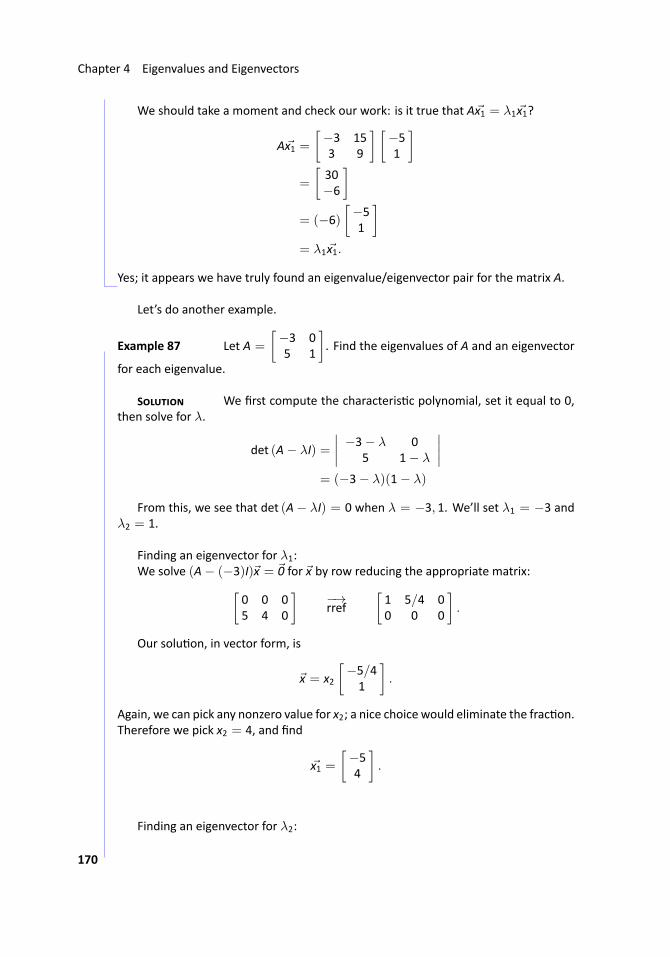
Chapter 4 Eigenvalues and Eigenvectors
We should take a moment and check our work: is it true that Ax1 = λ1x1?
Ax1 =[−3 153 9
] [−51
]=
[30−6
]= (−6)
[−51
]= λ1x1.
Yes; it appears we have truly found an eigenvalue/eigenvector pair for the matrix A. ...
Let’s do another example.
.. Example 87 ..Let A =
[−3 05 1
]. Find the eigenvalues of A and an eigenvector
for each eigenvalue.
S We first compute the characteris c polynomial, set it equal to 0,then solve for λ.
det (A− λI) =
∣∣∣∣ −3− λ 05 1− λ
∣∣∣∣= (−3− λ)(1− λ)
From this, we see that det (A− λI) = 0 when λ = −3, 1. We’ll set λ1 = −3 andλ2 = 1.
Finding an eigenvector for λ1:We solve (A− (−3)I)x = 0 for x by row reducing the appropriate matrix:[
0 0 05 4 0
]−→rref
[1 5/4 00 0 0
].
Our solu on, in vector form, is
x = x2
[−5/41
].
Again, we can pick any nonzero value for x2; a nice choice would eliminate the frac on.Therefore we pick x2 = 4, and find
x1 =[−54
].
Finding an eigenvector for λ2:
170
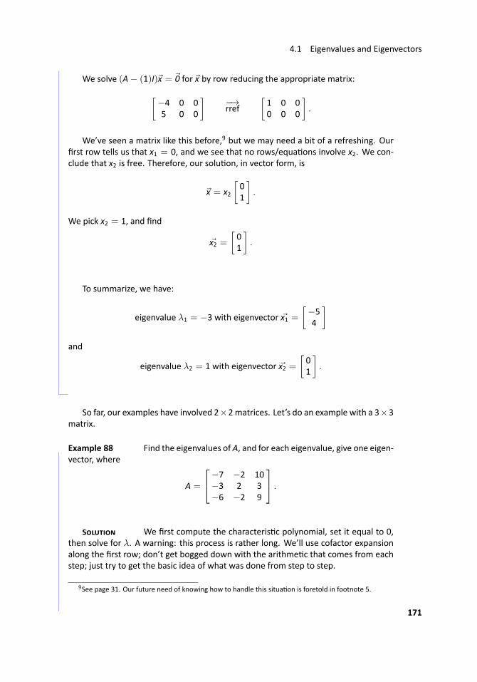
4.1 Eigenvalues and Eigenvectors
We solve (A− (1)I)x = 0 for x by row reducing the appropriate matrix:[−4 0 05 0 0
]−→rref
[1 0 00 0 0
].
We’ve seen a matrix like this before,9 but we may need a bit of a refreshing. Ourfirst row tells us that x1 = 0, and we see that no rows/equa ons involve x2. We con-clude that x2 is free. Therefore, our solu on, in vector form, is
x = x2
[01
].
We pick x2 = 1, and find
x2 =[01
].
To summarize, we have:
eigenvalue λ1 = −3 with eigenvector x1 =[−54
]and
eigenvalue λ2 = 1 with eigenvector x2 =[01
].
...
So far, our examples have involved 2×2matrices. Let’s do an example with a 3×3matrix.
.. Example 88 ..Find the eigenvalues of A, and for each eigenvalue, give one eigen-vector, where
A =
−7 −2 10−3 2 3−6 −2 9
.
S We first compute the characteris c polynomial, set it equal to 0,then solve for λ. A warning: this process is rather long. We’ll use cofactor expansionalong the first row; don’t get bogged down with the arithme c that comes from eachstep; just try to get the basic idea of what was done from step to step.
9See page 31. Our future need of knowing how to handle this situa on is foretold in footnote 5.
171
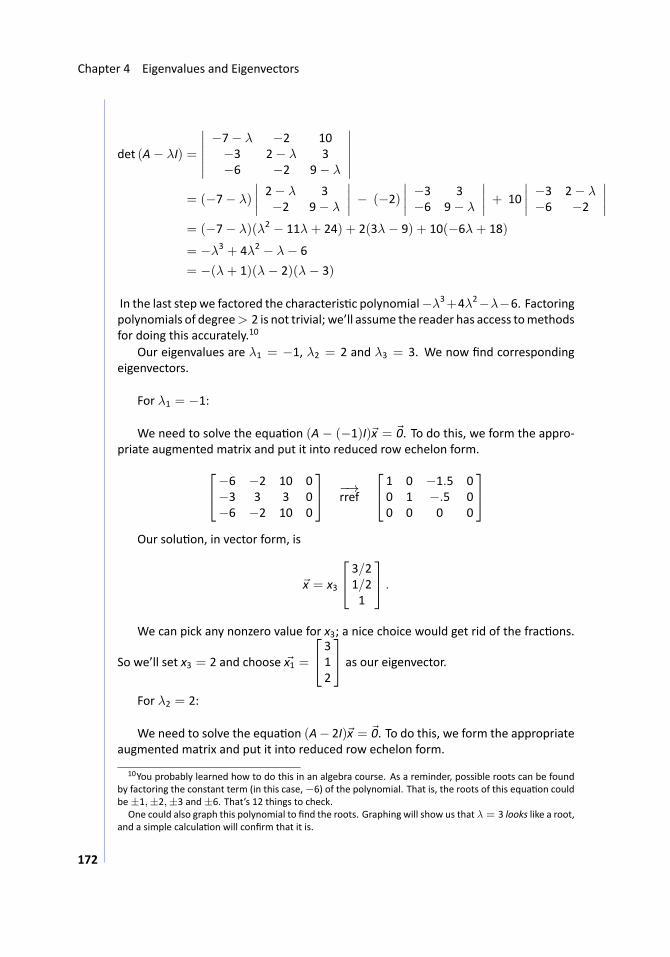
Chapter 4 Eigenvalues and Eigenvectors
det (A− λI) =
∣∣∣∣∣∣−7− λ −2 10−3 2− λ 3−6 −2 9− λ
∣∣∣∣∣∣= (−7− λ)
∣∣∣∣ 2− λ 3−2 9− λ
∣∣∣∣ − (−2)
∣∣∣∣ −3 3−6 9− λ
∣∣∣∣ + 10
∣∣∣∣ −3 2− λ−6 −2
∣∣∣∣= (−7− λ)(λ2 − 11λ+ 24) + 2(3λ− 9) + 10(−6λ+ 18)
= −λ3 + 4λ2 − λ− 6
= −(λ+ 1)(λ− 2)(λ− 3)
..In the last stepwe factored the characteris c polynomial−λ3+4λ2−λ−6. Factoringpolynomials of degree> 2 is not trivial; we’ll assume the reader has access tomethodsfor doing this accurately.10
Our eigenvalues are λ1 = −1, λ2 = 2 and λ3 = 3. We now find correspondingeigenvectors.
For λ1 = −1:
We need to solve the equa on (A − (−1)I)x = 0. To do this, we form the appro-priate augmented matrix and put it into reduced row echelon form.−6 −2 10 0
−3 3 3 0−6 −2 10 0
−→rref
1 0 −1.5 00 1 −.5 00 0 0 0
Our solu on, in vector form, is
x = x3
3/21/21
.
We can pick any nonzero value for x3; a nice choice would get rid of the frac ons.
So we’ll set x3 = 2 and choose x1 =
312
as our eigenvector.
For λ2 = 2:
We need to solve the equa on (A− 2I)x = 0. To do this, we form the appropriateaugmented matrix and put it into reduced row echelon form.
10You probably learned how to do this in an algebra course. As a reminder, possible roots can be foundby factoring the constant term (in this case,−6) of the polynomial. That is, the roots of this equa on couldbe±1,±2,±3 and±6. That’s 12 things to check.
One could also graph this polynomial to find the roots. Graphing will show us that λ = 3 looks like a root,and a simple calcula on will confirm that it is.
172
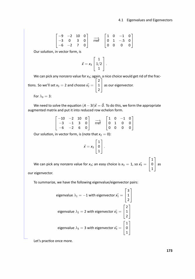
4.1 Eigenvalues and Eigenvectors
−9 −2 10 0−3 0 3 0−6 −2 7 0
−→rref
1 0 −1 00 1 −.5 00 0 0 0
Our solu on, in vector form, is
x = x3
11/21
.
We can pick any nonzero value for x3; again, a nice choice would get rid of the frac-
ons. So we’ll set x3 = 2 and choose x2 =
212
as our eigenvector.
For λ3 = 3:
We need to solve the equa on (A− 3I)x = 0. To do this, we form the appropriateaugmented matrix and put it into reduced row echelon form.−10 −2 10 0
−3 −1 3 0−6 −2 6 0
−→rref
1 0 −1 00 1 0 00 0 0 0
Our solu on, in vector form, is (note that x2 = 0):
x = x3
101
.
We can pick any nonzero value for x3; an easy choice is x3 = 1, so x3 =
101
as
our eigenvector.
To summarize, we have the following eigenvalue/eigenvector pairs:
eigenvalue λ1 = −1 with eigenvector x1 =
312
eigenvalue λ2 = 2 with eigenvector x2 =
212
eigenvalue λ3 = 3 with eigenvector x3 =
101
...
Let’s prac ce once more.
173
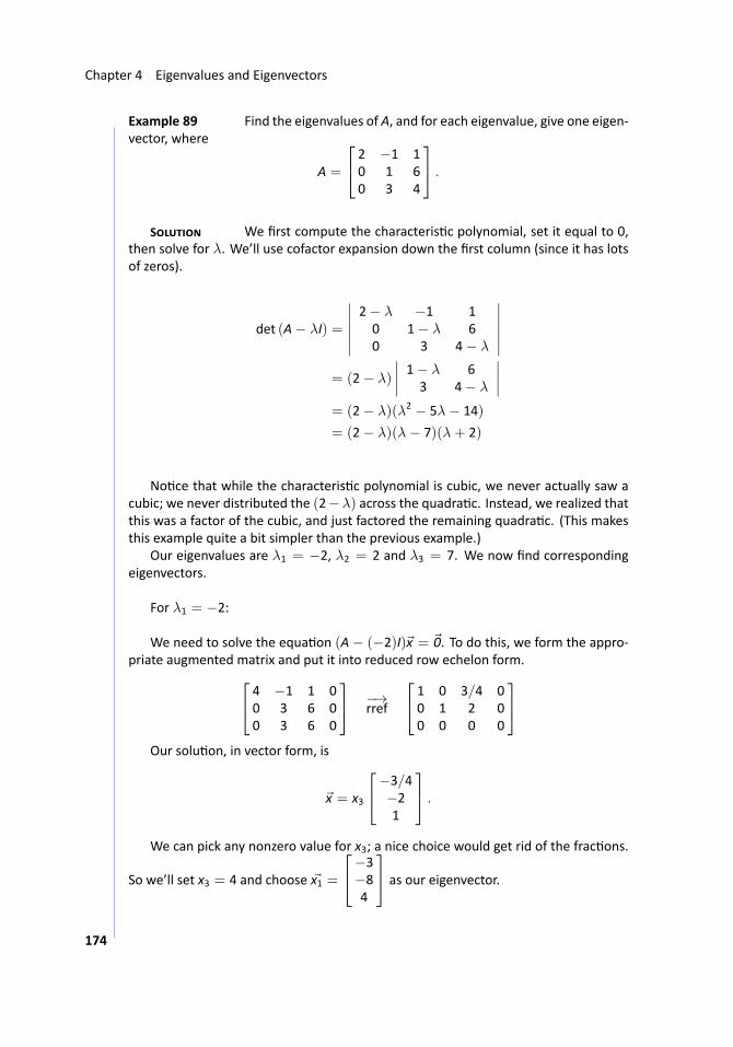
Chapter 4 Eigenvalues and Eigenvectors
.. Example 89 ..Find the eigenvalues of A, and for each eigenvalue, give one eigen-vector, where
A =
2 −1 10 1 60 3 4
.
S We first compute the characteris c polynomial, set it equal to 0,then solve for λ. We’ll use cofactor expansion down the first column (since it has lotsof zeros).
det (A− λI) =
∣∣∣∣∣∣2− λ −1 10 1− λ 60 3 4− λ
∣∣∣∣∣∣= (2− λ)
∣∣∣∣ 1− λ 63 4− λ
∣∣∣∣= (2− λ)(λ2 − 5λ− 14)
= (2− λ)(λ− 7)(λ+ 2)
No ce that while the characteris c polynomial is cubic, we never actually saw acubic; we never distributed the (2−λ) across the quadra c. Instead, we realized thatthis was a factor of the cubic, and just factored the remaining quadra c. (This makesthis example quite a bit simpler than the previous example.)
Our eigenvalues are λ1 = −2, λ2 = 2 and λ3 = 7. We now find correspondingeigenvectors.
For λ1 = −2:
We need to solve the equa on (A − (−2)I)x = 0. To do this, we form the appro-priate augmented matrix and put it into reduced row echelon form. 4 −1 1 0
0 3 6 00 3 6 0
−→rref
1 0 3/4 00 1 2 00 0 0 0
Our solu on, in vector form, is
x = x3
−3/4−21
.
We can pick any nonzero value for x3; a nice choice would get rid of the frac ons.
So we’ll set x3 = 4 and choose x1 =
−3−84
as our eigenvector.
174
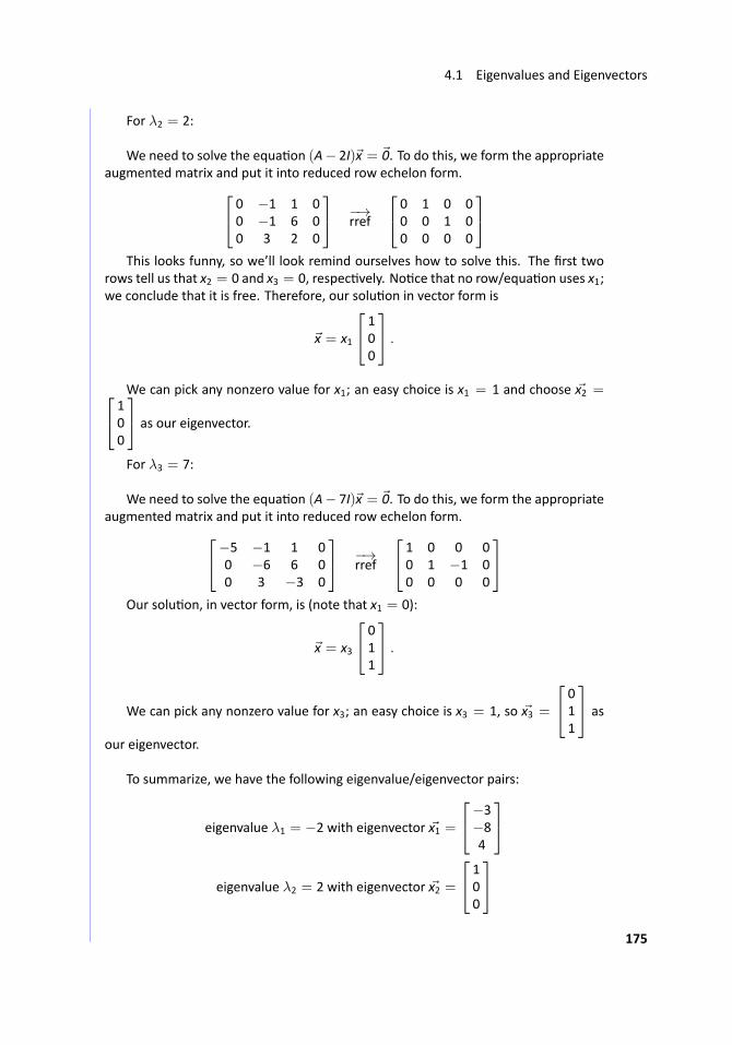
4.1 Eigenvalues and Eigenvectors
For λ2 = 2:
We need to solve the equa on (A− 2I)x = 0. To do this, we form the appropriateaugmented matrix and put it into reduced row echelon form. 0 −1 1 0
0 −1 6 00 3 2 0
−→rref
0 1 0 00 0 1 00 0 0 0
This looks funny, so we’ll look remind ourselves how to solve this. The first two
rows tell us that x2 = 0 and x3 = 0, respec vely. No ce that no row/equa on uses x1;we conclude that it is free. Therefore, our solu on in vector form is
x = x1
100
.
..We can pick any nonzero value for x1; an easy choice is x1 = 1 and choose x2 = 1
00
as our eigenvector.
For λ3 = 7:
We need to solve the equa on (A− 7I)x = 0. To do this, we form the appropriateaugmented matrix and put it into reduced row echelon form.−5 −1 1 0
0 −6 6 00 3 −3 0
−→rref
1 0 0 00 1 −1 00 0 0 0
Our solu on, in vector form, is (note that x1 = 0):
x = x3
011
.
We can pick any nonzero value for x3; an easy choice is x3 = 1, so x3 =
011
as
our eigenvector.
To summarize, we have the following eigenvalue/eigenvector pairs:
eigenvalue λ1 = −2 with eigenvector x1 =
−3−84
eigenvalue λ2 = 2 with eigenvector x2 =
100
175
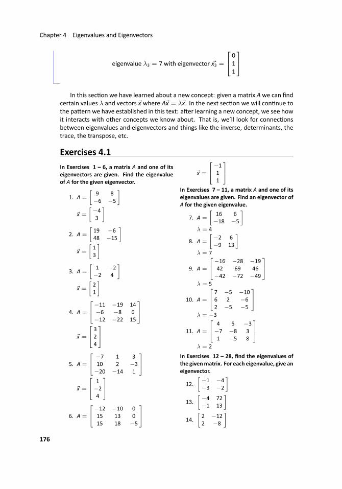
Chapter 4 Eigenvalues and Eigenvectors
eigenvalue λ3 = 7 with eigenvector x3 =
011
...
In this sec on we have learned about a new concept: given a matrix Awe can findcertain values λ and vectors x where Ax = λx. In the next sec on we will con nue tothe pa ern we have established in this text: a er learning a new concept, we see howit interacts with other concepts we know about. That is, we’ll look for connec onsbetween eigenvalues and eigenvectors and things like the inverse, determinants, thetrace, the transpose, etc.
Exercises 4.1In Exercises 1 – 6, a matrix A and one of itseigenvectors are given. Find the eigenvalueof A for the given eigenvector.
1. A =
[9 8−6 −5
]x =
[−43
]
2. A =
[19 −648 −15
]x =
[13
]
3. A =
[1 −2−2 4
]x =
[21
]
4. A =
−11 −19 14−6 −8 6−12 −22 15
x =
324
5. A =
−7 1 310 2 −3−20 −14 1
x =
1−24
6. A =
−12 −10 015 13 015 18 −5
x =
−111
In Exercises 7 – 11, a matrix A and one of itseigenvalues are given. Find an eigenvector ofA for the given eigenvalue.
7. A =
[16 6−18 −5
]λ = 4
8. A =
[−2 6−9 13
]λ = 7
9. A =
−16 −28 −1942 69 46−42 −72 −49
λ = 5
10. A =
7 −5 −106 2 −62 −5 −5
λ = −3
11. A =
4 5 −3−7 −8 31 −5 8
λ = 2
In Exercises 12 – 28, find the eigenvalues ofthe givenmatrix. For each eigenvalue, give aneigenvector.
12.[−1 −4−3 −2
]13.
[−4 72−1 13
]14.
[2 −122 −8
]176
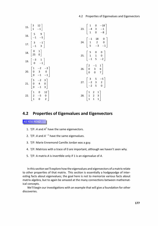
4.2 Proper es of Eigenvalues and Eigenvectors
15.[3 121 −1
]16.
[5 9−1 −5
]17.
[3 −1−1 3
]18.
[0 125 0
]19.
[−3 10 −1
]
20.
1 −2 −30 3 00 −1 −1
21.
5 −2 30 4 00 −1 3
22.
1 0 122 −5 01 0 2
23.
1 0 −18−4 3 −11 0 −8
24.
−1 18 01 2 05 −3 −1
25.
5 0 01 1 0−1 5 −2
26.
2 −1 10 3 60 0 7
27.
3 5 −5−2 3 2−2 5 0
28.
1 2 11 2 31 1 1
4.2 Proper es of Eigenvalues and Eigenvectors
...AS YOU READ . . .
1. T/F: A and AT have the same eigenvectors.
2. T/F: A and A−1 have the same eigenvalues.
3. T/F: Marie Ennemond Camille Jordan was a guy.
4. T/F: Matrices with a trace of 0 are important, although we haven’t seen why.
5. T/F: A matrix A is inver ble only if 1 is an eigenvalue of A.
In this sec onwe’ll explore how the eigenvalues and eigenvectors of amatrix relateto other proper es of that matrix. This sec on is essen ally a hodgepodge of inter-es ng facts about eigenvalues; the goal here is not to memorize various facts aboutmatrix algebra, but to again be amazed at the many connec ons between mathemat-ical concepts.
We’ll begin our inves ga ons with an example that will give a founda on for otherdiscoveries.
177
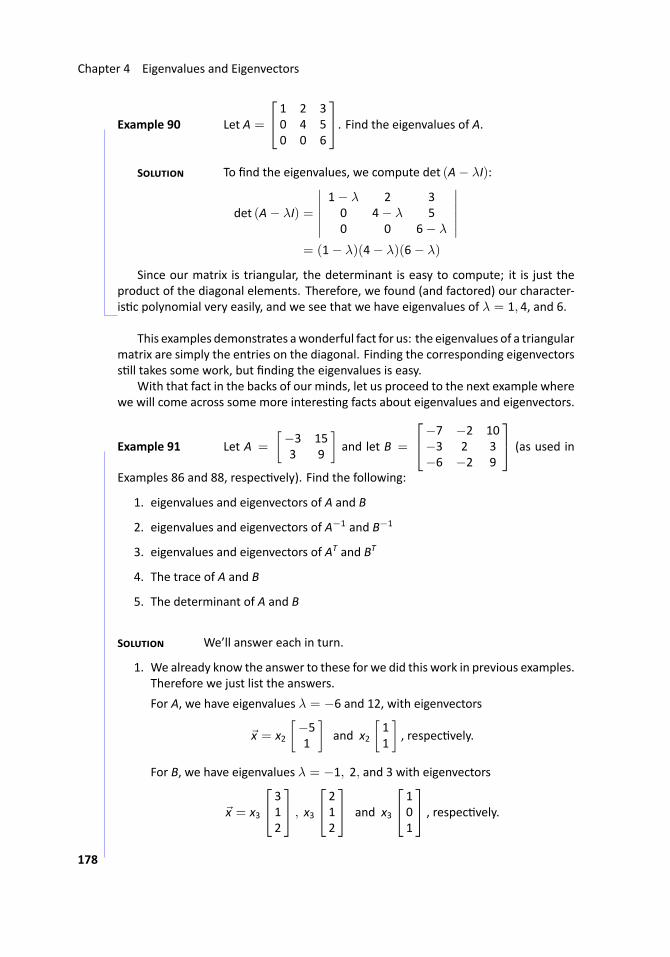
Chapter 4 Eigenvalues and Eigenvectors
.. Example 90 Let A =
1 2 30 4 50 0 6
. Find the eigenvalues of A.
S To find the eigenvalues, we compute det (A− λI):
det (A− λI) =
∣∣∣∣∣∣1− λ 2 30 4− λ 50 0 6− λ
∣∣∣∣∣∣= (1− λ)(4− λ)(6− λ)
Since our matrix is triangular, the determinant is easy to compute; it is just theproduct of the diagonal elements. Therefore, we found (and factored) our character-is c polynomial very easily, and we see that we have eigenvalues of λ = 1, 4, and 6. ..
This examples demonstrates awonderful fact for us: the eigenvalues of a triangularmatrix are simply the entries on the diagonal. Finding the corresponding eigenvectorss ll takes some work, but finding the eigenvalues is easy.
With that fact in the backs of our minds, let us proceed to the next example wherewe will come across some more interes ng facts about eigenvalues and eigenvectors.
.. Example 91 ..Let A =
[−3 153 9
]and let B =
−7 −2 10−3 2 3−6 −2 9
(as used in
Examples 86 and 88, respec vely). Find the following:
1. eigenvalues and eigenvectors of A and B
2. eigenvalues and eigenvectors of A−1 and B−1
3. eigenvalues and eigenvectors of AT and BT
4. The trace of A and B
5. The determinant of A and B
S We’ll answer each in turn.
1. We already know the answer to these for we did this work in previous examples.Therefore we just list the answers.
For A, we have eigenvalues λ = −6 and 12, with eigenvectors
x = x2
[−51
]and x2
[11
], respec vely.
For B, we have eigenvalues λ = −1, 2, and 3 with eigenvectors
x = x3
312
, x3
212
and x3
101
, respec vely.
178
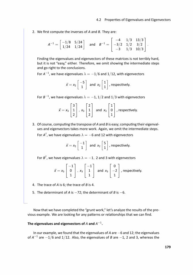
4.2 Proper es of Eigenvalues and Eigenvectors
2. We first compute the inverses of A and B. They are:
A−1 =
[−1/8 5/241/24 1/24
]and B−1 =
−4 1/3 13/3−3/2 1/2 3/2−3 1/3 10/3
.
Finding the eigenvalues and eigenvectors of these matrices is not terribly hard,but it is not “easy,” either. Therefore, we omit showing the intermediate stepsand go right to the conclusions.
For A−1, we have eigenvalues λ = −1/6 and 1/12, with eigenvectors
x = x2
[−51
]and x2
[11
], respec vely.
For B−1, we have eigenvalues λ = −1, 1/2 and 1/3 with eigenvectors
x = x3
312
, x3
212
and x3
101
, respec vely.
3. Of course, compu ng the transpose of A and B is easy; compu ng their eigenval-ues and eigenvectors takes more work. Again, we omit the intermediate steps.
For AT, we have eigenvalues λ = −6 and 12 with eigenvectors
x = x2
[−11
]and x2
[51
], respec vely.
For BT, we have eigenvalues λ = −1, 2 and 3 with eigenvectors
x = x3
−101
, x3
−111
and x3
0−21
, respec vely.
4. The trace of A is 6; the trace of B is 4.
5. The determinant of A is−72; the determinant of B is−6.
...
Now that we have completed the “grunt work,” let’s analyze the results of the pre-vious example. We are looking for any pa erns or rela onships that we can find.
The eigenvalues and eigenvectors of A and A−1.
In our example, we found that the eigenvalues of A are−6 and 12; the eigenvaluesof A−1 are −1/6 and 1/12. Also, the eigenvalues of B are −1, 2 and 3, whereas the
179
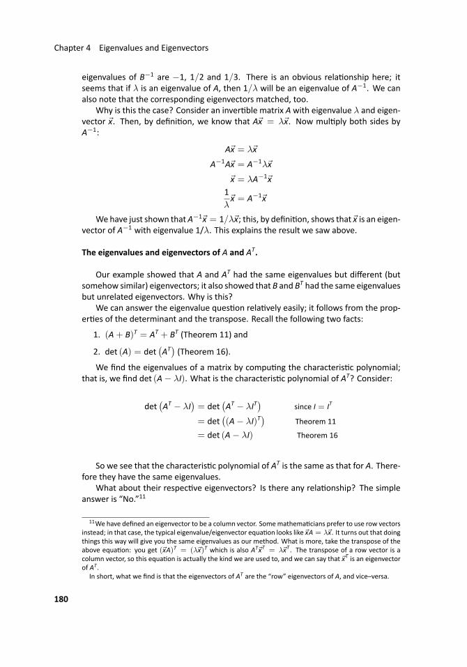
Chapter 4 Eigenvalues and Eigenvectors
eigenvalues of B−1 are −1, 1/2 and 1/3. There is an obvious rela onship here; itseems that if λ is an eigenvalue of A, then 1/λ will be an eigenvalue of A−1. We canalso note that the corresponding eigenvectors matched, too.
Why is this the case? Consider an inver ble matrix Awith eigenvalue λ and eigen-vector x. Then, by defini on, we know that Ax = λx. Now mul ply both sides byA−1:
Ax = λx
A−1Ax = A−1λx
x = λA−1x1λx = A−1x
Wehave just shown thatA−1x = 1/λx; this, by defini on, shows that x is an eigen-vector of A−1 with eigenvalue 1/λ. This explains the result we saw above.
The eigenvalues and eigenvectors of A and AT.
Our example showed that A and AT had the same eigenvalues but different (butsomehow similar) eigenvectors; it also showed that B and BT had the same eigenvaluesbut unrelated eigenvectors. Why is this?
We can answer the eigenvalue ques on rela vely easily; it follows from the prop-er es of the determinant and the transpose. Recall the following two facts:
1. (A+ B)T = AT + BT (Theorem 11) and
2. det (A) = det(AT)(Theorem 16).
We find the eigenvalues of a matrix by compu ng the characteris c polynomial;that is, we find det (A− λI). What is the characteris c polynomial of AT? Consider:
det(AT − λI
)= det
(AT − λIT
)since I = IT
= det((A− λI)T
)Theorem 11
= det (A− λI) Theorem 16
So we see that the characteris c polynomial of AT is the same as that for A. There-fore they have the same eigenvalues.
What about their respec ve eigenvectors? Is there any rela onship? The simpleanswer is “No.”11
11We have defined an eigenvector to be a column vector. Somemathema cians prefer to use row vectorsinstead; in that case, the typical eigenvalue/eigenvector equa on looks like xA = λx. It turns out that doingthings this way will give you the same eigenvalues as our method. What is more, take the transpose of theabove equa on: you get (xA)T = (λx)T which is also ATxT = λxT. The transpose of a row vector is acolumn vector, so this equa on is actually the kind we are used to, and we can say that xT is an eigenvectorof AT.
In short, what we find is that the eigenvectors of AT are the “row” eigenvectors of A, and vice–versa.
180
4.2 Proper es of Eigenvalues and Eigenvectors
The eigenvalues and eigenvectors of A and The Trace.
Note that the eigenvalues of A are −6 and 12, and the trace is 6; the eigenvaluesof B are−1, 2 and 3, and the trace of B is 4. Do we no ce any rela onship?
It seems that the sum of the eigenvalues is the trace! Why is this the case?
The answer to this is a bit out of the scope of this text; we can jus fy part of thisfact, and another part we’ll just state as being true without jus fica on.
First, recall from Theorem 13 that tr(AB) =tr(BA). Secondly, we state without jus-fica on that given a squarematrix A, we can find a squarematrix P such that P−1AP is
an upper triangularmatrixwith the eigenvalues ofA on the diagonal.12 Thus tr(P−1AP)is the sum of the eigenvalues; also, using our Theorem 13, we know that tr(P−1AP) =tr(P−1PA) = tr(A). Thus the trace of A is the sum of the eigenvalues.
The eigenvalues and eigenvectors of A and The Determinant.
Again, the eigenvalues of A are −6 and 12, and the determinant of A is −72. Theeigenvalues of B are −1, 2 and 3; the determinant of B is −6. It seems as though theproduct of the eigenvalues is the determinant.
This is indeed true; we defend this with our argument from above. We know thatthe determinant of a triangular matrix is the product of the diagonal elements. There-fore, given a matrix A, we can find P such that P−1AP is upper triangular with theeigenvalues of A on the diagonal. Thus det
(P−1AP
)is the product of the eigenvalues.
Using Theorem 16, we know that det(P−1AP
)= det
(P−1PA
)= det (A). Thus the
determinant of A is the product of the eigenvalues.
We summarize the results of our example with the following theorem.
12Who in the world thinks up this stuff? It seems that the answer is Marie Ennemond Camille Jordan,who, despite having at least two girl names, was a guy.
181
Chapter 4 Eigenvalues and Eigenvectors
..Theorem 19
.
.Proper es of Eigenvalues and Eigenvectors
Let A be an n× n inver ble matrix. The following are true:
1. If A is triangular, then the diagonal elements of A arethe eigenvalues of A.
2. If λ is an eigenvalue of Awith eigenvector x, then 1λ is
an eigenvalue of A−1 with eigenvector x.
3. If λ is an eigenvalue of A then λ is an eigenvalue ofAT.
4. The sum of the eigenvalues of A is equal to tr(A), thetrace of A.
5. The product of the eigenvalues of A is the equal todet (A), the determinant of A.
There is one more concept concerning eigenvalues and eigenvectors that we willexplore. We do so in the context of an example.
.. Example 92 ..Find the eigenvalues and eigenvectors of thematrixA =
[1 21 2
].
S To find the eigenvalues, we compute det (A− λI):
det (A− λI) =
∣∣∣∣ 1− λ 21 2− λ
∣∣∣∣= (1− λ)(2− λ)− 2
= λ2 − 3λ
= λ(λ− 3)
Our eigenvalues are therefore λ = 0, 3.For λ = 0, we find the eigenvectors:[
1 2 01 2 0
]−→rref
[1 2 00 0 0
]This shows that x1 = −2x2, and so our eigenvectors x are
x = x2
[−21
].
For λ = 3, we find the eigenvectors:
182
4.2 Proper es of Eigenvalues and Eigenvectors
[−2 2 01 −1 0
]−→rref
[1 −1 00 0 0
]This shows that x1 = x2, and so our eigenvectors x are
x = x2
[11
].
...
One interes ng thing about the above example is that we see that 0 is an eigen-value of A; we have not officially encountered this before. Does this mean anythingsignificant?13
Think aboutwhat an eigenvalue of 0means: there exists an nonzero vector xwhereAx = 0x = 0. That is, we have a nontrivial solu on to Ax = 0. We know this onlyhappens when A is not inver ble.
So if A is inver ble, there is no nontrivial solu on to Ax = 0, and hence 0 is notan eigenvalue of A. If A is not inver ble, then there is a nontrivial solu on to Ax = 0,and hence 0 is an eigenvalue of A. This leads us to our final addi on to the Inver bleMatrix Theorem.
..Theorem 20
.
.Inver ble Matrix Theorem
LetA be an n×nmatrix. The following statements are equiv-alent.
(a) A is inver ble.
(h) A does not have an eigenvalue of 0.
This sec on is about the proper es of eigenvalues and eigenvectors. Of course, wehave not inves gated all of the numerous proper es of eigenvalues and eigenvectors;we have just surveyed some of the most common (and most important) concepts.Here are four quick examples of the many things that s ll exist to be explored.
First, recall the matrix
A =
[1 42 3
]that we used in Example 84. It’s characteris c polynomial is p(λ) = λ2 − 4λ − 5.Compute p(A); that is, compute A2−4A−5I. You should get something “interes ng,”and you should wonder “does this always work?”14
13Since 0 is a “special” number, we might think so – a erall, we found that having a determinant of 0 isimportant. Then again, a matrix with a trace of 0 isn’t all that important. (Well, as far as we have seen; itactually is). So, having an eigenvalue of 0 may or may not be significant, but we would be doing well if werecognized the possibility of significance and decided to inves gate further.
14Yes.
183
Chapter 4 Eigenvalues and Eigenvectors
Second, in all of our examples, we have considered matrices where eigenvalues“appeared only once.” Since we know that the eigenvalues of a triangular matrix ap-pear on the diagonal, we know that the eigenvalues of
A =
[1 10 1
]are “1 and 1;” that is, the eigenvalue λ = 1 appears twice. What does thatmeanwhenwe consider the eigenvectors of λ = 1? Compare the result of this to the matrix
A =
[1 00 1
],
which also has the eigenvalue λ = 1 appearing twice.15
Third, consider the matrix
A =
[0 −11 0
].
What are the eigenvalues?16 We quickly compute the characteris c polynomial to bep(λ) = λ2 + 1. Therefore the eigenvalues are±
√−1 = ±i. What does this mean?
Finally, we have found the eigenvalues of matrices by finding the roots of the char-acteris c polynomial. We have limited our examples to quadra c and cubic polynomi-als; onewould expect for larger sizedmatrices that a computerwould be used to factorthe characteris c polynomials. However, in general, this is not how the eigenvaluesare found. Factoring high order polynomials is too unreliable, even with a computer– round off errors can cause unpredictable results. Also, to even compute the charac-teris c polynomial, one needs to compute the determinant, which is also expensive(as discussed in the previous chapter).
So how are eigenvalues found? There are itera ve processes that can progressivelytransform amatrix A into another matrix that is almost an upper triangular matrix (theentries below the diagonal are almost zero) where the entries on the diagonal are theeigenvalues. The more itera ons one performs, the be er the approxima on is.
Thesemethods are so fast and reliable that some computer programs convert poly-nomial root finding problems into eigenvalue problems!
Most textbooks on Linear Algebra will provide direc on on exploring the abovetopics and give further insight to what is going on. We have men oned all the eigen-value and eigenvector proper es in this sec on for the same reasons we gave in theprevious sec on. First, knowing these proper es helps us solve numerous real worldproblems, and second, it is fascina ng to see how rich and deep the theory of matricesis.
15To direct further study, it helps to know that mathema cians refer to this as the duplicity of an eigen-value. In each of these two examples, A has the eigenvalue λ = 1 with duplicity of 2.
16Be careful; this matrix is not triangular.
184
4.2 Proper es of Eigenvalues and Eigenvectors
Exercises 4.2In Exercises 1 – 6, a matrix A is given. Foreach,
(a) Find the eigenvalues of A, and for eacheigenvalue, find an eigenvector.
(b) Do the same for AT.
(c) Do the same for A−1.
(d) Find tr(A).
(e) Find det (A).
Use Theorem 19 to verify your results.
1.[
0 4−1 5
]
2.[−2 −14−1 3
]3.
[5 30−1 −6
]4.
[−4 72−1 13
]
5.
5 −9 01 −5 02 4 3
6.
0 25 01 0 01 1 −3
185

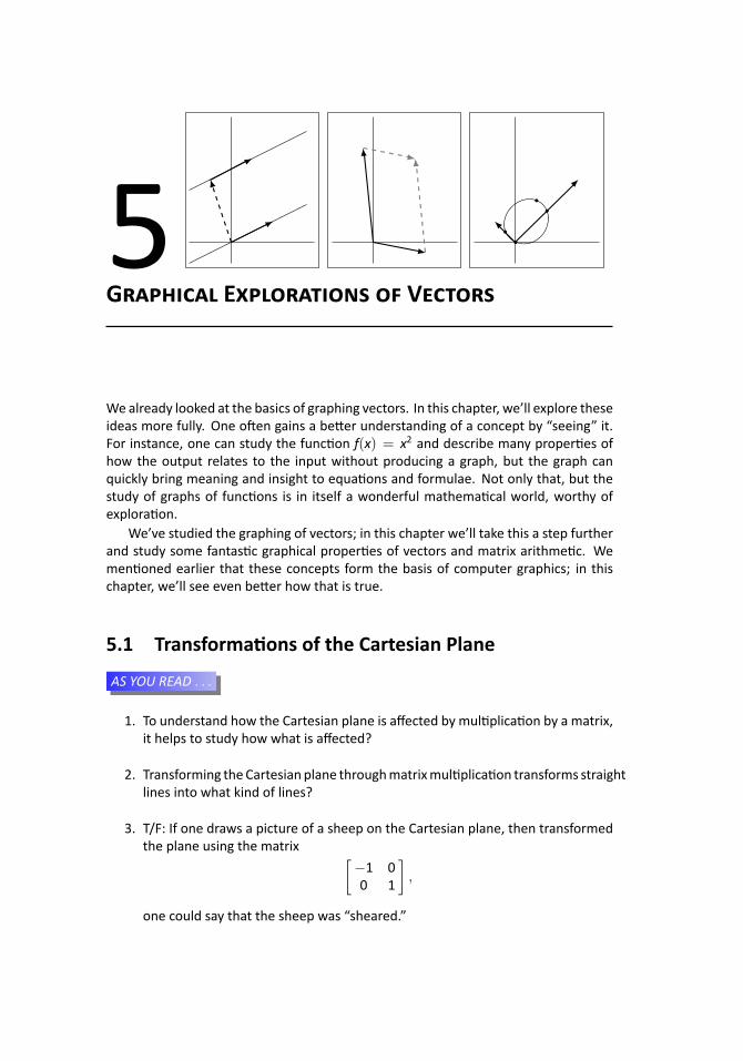
5 .
G E V
Wealready looked at the basics of graphing vectors. In this chapter, we’ll explore theseideas more fully. One o en gains a be er understanding of a concept by “seeing” it.For instance, one can study the func on f(x) = x2 and describe many proper es ofhow the output relates to the input without producing a graph, but the graph canquickly bring meaning and insight to equa ons and formulae. Not only that, but thestudy of graphs of func ons is in itself a wonderful mathema cal world, worthy ofexplora on.
We’ve studied the graphing of vectors; in this chapter we’ll take this a step furtherand study some fantas c graphical proper es of vectors and matrix arithme c. Wemen oned earlier that these concepts form the basis of computer graphics; in thischapter, we’ll see even be er how that is true.
5.1 Transforma ons of the Cartesian Plane
...AS YOU READ . . .
1. To understand how the Cartesian plane is affected by mul plica on by a matrix,it helps to study how what is affected?
2. Transforming theCartesian plane throughmatrixmul plica on transforms straightlines into what kind of lines?
3. T/F: If one draws a picture of a sheep on the Cartesian plane, then transformedthe plane using the matrix [
−1 00 1
],
one could say that the sheep was “sheared.”
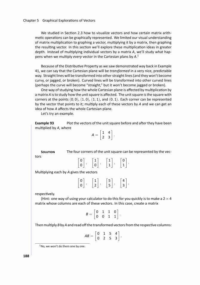
Chapter 5 Graphical Explora ons of Vectors
We studied in Sec on 2.3 how to visualize vectors and how certain matrix arith-me c opera ons can be graphically represented. We limited our visual understandingof matrix mul plica on to graphing a vector, mul plying it by a matrix, then graphingthe resul ng vector. In this sec on we’ll explore these mul plica on ideas in greaterdepth. Instead of mul plying individual vectors by a matrix A, we’ll study what hap-pens when we mul ply every vector in the Cartesian plans by A.1
Because of the Distribu ve Property as we saw demonstrated way back in Example41, we can say that the Cartesian plane will be transformed in a very nice, predictableway. Straight lineswill be transformed into other straight lines (and theywon’t becomecurvy, or jagged, or broken). Curved lines will be transformed into other curved lines(perhaps the curve will become “straight,” but it won’t become jagged or broken).
Oneway of studying how thewhole Cartesian plane is affected bymul plica on byamatrixA is to study how the unit square is affected. The unit square is the squarewithcorners at the points (0, 0), (1, 0), (1, 1), and (0, 1). Each corner can be representedby the vector that points to it; mul ply each of these vectors by A and we can get anidea of how A affects the whole Cartesian plane.
Let’s try an example.
.. Example 93 ..Plot the vectors of the unit square before and a er they have beenmul plied by A, where
A =
[1 42 3
].
S The four corners of the unit square can be represented by the vec-tors [
00
],
[10
],
[11
],
[01
].
Mul plying each by A gives the vectors[00
],
[12
],
[55
],
[43
],
respec vely.(Hint: one way of using your calculator to do this for you quickly is to make a 2× 4
matrix whose columns are each of these vectors. In this case, create a matrix
B =
[0 1 1 00 0 1 1
].
Thenmul plyBbyA and readoff the transformed vectors from the respec ve columns:
AB =
[0 1 5 40 2 5 3
].
1No, we won’t do them one by one.
188
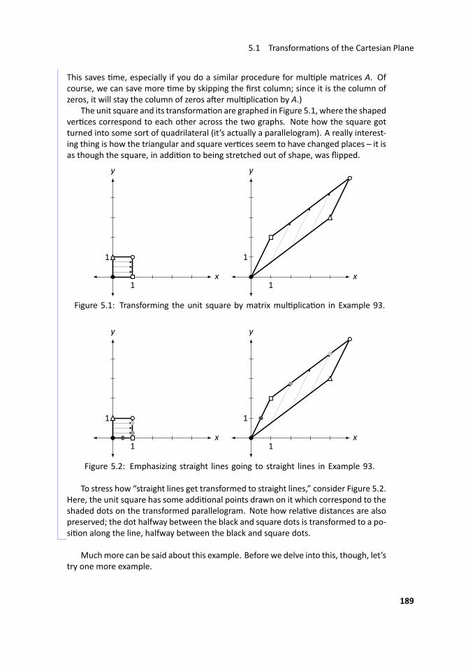
5.1 Transforma ons of the Cartesian Plane
This saves me, especially if you do a similar procedure for mul ple matrices A. Ofcourse, we can save more me by skipping the first column; since it is the column ofzeros, it will stay the column of zeros a er mul plica on by A.)
The unit square and its transforma on are graphed in Figure 5.1, where the shapedver ces correspond to each other across the two graphs. Note how the square gotturned into some sort of quadrilateral (it’s actually a parallelogram). A really interest-ing thing is how the triangular and square ver ces seem to have changed places – it isas though the square, in addi on to being stretched out of shape, was flipped.
.. x.
y
.1
.
1
..... x.
y
.1
.
1
....
..Figure 5.1: Transforming the unit square by matrix mul plica on in Example 93.
.. x.
y
.1
.
1
..... x.
y
.1
.
1
....
..Figure 5.2: Emphasizing straight lines going to straight lines in Example 93.
To stress how “straight lines get transformed to straight lines,” consider Figure 5.2.Here, the unit square has some addi onal points drawn on it which correspond to theshaded dots on the transformed parallelogram. Note how rela ve distances are alsopreserved; the dot halfway between the black and square dots is transformed to a po-si on along the line, halfway between the black and square dots. ...
Muchmore can be said about this example. Before we delve into this, though, let’stry one more example.
189
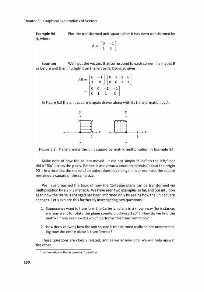
Chapter 5 Graphical Explora ons of Vectors
.. Example 94 Plot the transformed unit square a er it has been transformed byA, where
A =
[0 −11 0
].
S We’ll put the vectors that correspond to each corner in a matrix Bas before and then mul ply it on the le by A. Doing so gives:
AB =
[0 −11 0
] [0 1 1 00 0 1 1
]=
[0 0 −1 −10 1 1 0
]In Figure 5.3 the unit square is again drawn along with its transforma on by A.
.. x.
y
.1
.
1
..... x.
y
.1
....
..Figure 5.3: Transforming the unit square by matrix mul plica on in Example 94.
Make note of how the square moved. It did not simply “slide” to the le ;2 nordid it “flip” across the y axis. Rather, it was rotated counterclockwise about the origin90◦. In a rota on, the shape of an object does not change; in our example, the squareremained a square of the same size. ..
We have broached the topic of how the Cartesian plane can be transformed viamul plica on by a 2×2matrix A. We have seen two examples so far, and our intui onas to how the plane is changed has been informed only by seeing how the unit squarechanges. Let’s explore this further by inves ga ng two ques ons:
1. Suppose wewant to transform the Cartesian plane in a knownway (for instance,we may want to rotate the plane counterclockwise 180◦). How do we find thematrix (if one even exists) which performs this transforma on?
2. Howdoes knowing how the unit square is transformed really help in understand-ing how the en re plane is transformed?
These ques ons are closely related, and as we answer one, we will help answerthe other.
2mathema cally, that is called a transla on
190
5.1 Transforma ons of the Cartesian Plane
To get started with the first ques on, look back at Examples 93 and 94 and con-sider again how the unit square was transformed. In par cular, is there any correla onbetween where the ver ces ended up and the matrix A?
If you are just reading on, and haven’t actually gone back and looked at the exam-ples, go back now and try tomake some sort of connec on. Otherwise – youmay havenoted some of the following things:
1. The zero vector (0, the “black” corner) never moved. That makes sense, though;A0 = 0.
2. The “square” corner, i.e., the corner corresponding to the vector[10
], is always
transformed to the vector in the first column of A!
3. Likewise, the “triangular” corner, i.e., the corner corresponding to the vector[01
], is always transformed to the vector in the second column of A!3
4. The “white dot” corner is always transformed to the sum of the two columnvectors of A.4
Let’s now take the me to understand these four points. The first point should beclear; 0will always be transformed to 0 viamatrixmul plica on. (Hence the hint in themiddle of Example 93, where we are told that we can ignore entering in the column ofzeros in the matrix B.)
We can understand the second and third points simultaneously. Let
A =
[a bc d
], e1 =
[10
]and e2 =
[01
].
What are Ae1 and Ae2?
Ae1 =[a bc d
] [10
]=
[ac
]
Ae2 =[a bc d
] [01
]=
[bd
]3Although this is less of a surprise, given the result of the previous point.4This observa on is a bit more obscure than the first three. It follows from the fact that this corner of
the unit square is the “sum” of the other two nonzero corners.
191
Chapter 5 Graphical Explora ons of Vectors
So bymeremechanics ofmatrixmul plica on, the square corner e1 is transformedto the first column of A, and the triangular corner e2 is transformed to the second col-umn of A. A similar argument demonstrates why the white dot corner is transformedto the sum of the columns of A.5
Revisit now the ques on “How do we find the matrix that performs a given trans-forma on on the Cartesian plane?” The answer follows from what we just did. Thinkabout the given transforma on and how it would transform the corners of the unitsquare. Make the first column of A the vector where e1 goes, and make the secondcolumn of A the vector where e2 goes.
Let’s prac ce this in the context of an example.
.. Example 95 ..Find thematrixA that flips the Cartesian plane about the x axis andthen stretches the plane horizontally by a factor of two.
S We first consider e1 =
[10
]. Where does this corner go to under
the given transforma on? Flipping the plane across the x axis does not change e1 at
all; stretching the plane sends e1 to[20
]. Therefore, the first column of A is
[20
].
Now consider e2 =
[01
]. Flipping the plane about the x axis sends e2 to the vec-
tor[
0−1
]; subsequently stretching the plane horizontally does not affect this vector.
Therefore the second column of A is[
0−1
].
Pu ng this together gives
A =
[2 00 −1
].
To help visualize this, consider Figure 5.4 where a shape is transformed under thismatrix. No ce how it is turned upside down and is stretched horizontally by a factorof two. (The gridlines are given as a visual aid.)
5Another way of looking at all of this is to consider what A · I is: of course, it is just A. What are thecolumns of I? Just e1 and e2.
192
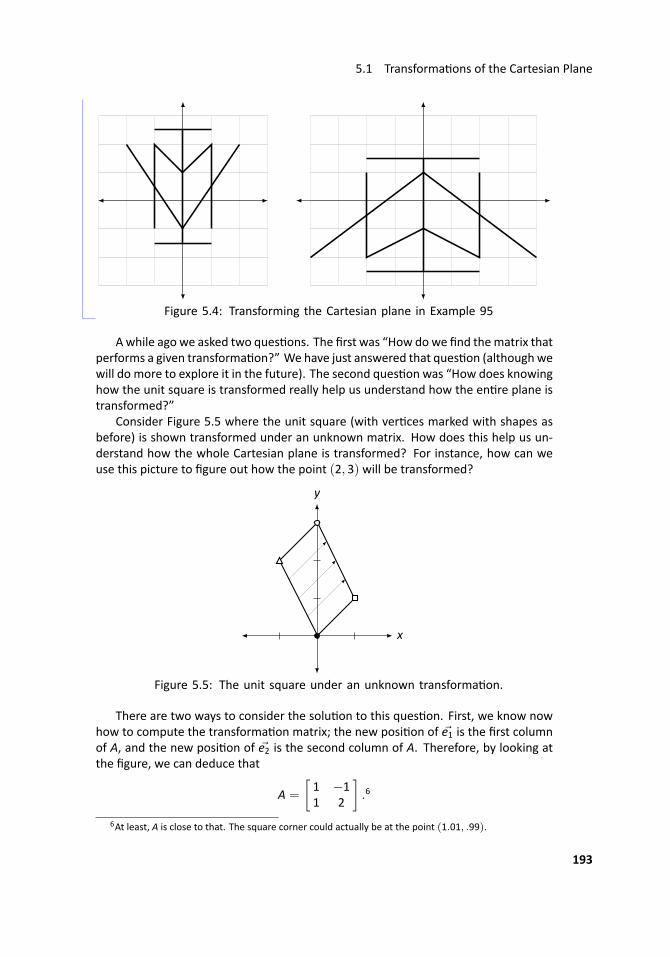
5.1 Transforma ons of the Cartesian Plane
.
..Figure 5.4: Transforming the Cartesian plane in Example 95...
A while ago we asked two ques ons. The first was “How dowe find thematrix thatperforms a given transforma on?” We have just answered that ques on (althoughwewill do more to explore it in the future). The second ques on was “How does knowinghow the unit square is transformed really help us understand how the en re plane istransformed?”
Consider Figure 5.5 where the unit square (with ver ces marked with shapes asbefore) is shown transformed under an unknown matrix. How does this help us un-derstand how the whole Cartesian plane is transformed? For instance, how can weuse this picture to figure out how the point (2, 3) will be transformed?
.. x.
y
....
..Figure 5.5: The unit square under an unknown transforma on.
There are two ways to consider the solu on to this ques on. First, we know nowhow to compute the transforma on matrix; the new posi on of e1 is the first columnof A, and the new posi on of e2 is the second column of A. Therefore, by looking atthe figure, we can deduce that
A =
[1 −11 2
].6
6At least, A is close to that. The square corner could actually be at the point (1.01, .99).
193
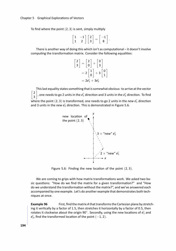
Chapter 5 Graphical Explora ons of Vectors
To find where the point (2, 3) is sent, simply mul ply[1 −11 2
] [23
]=
[−18
].
There is another way of doing this which isn’t as computa onal – it doesn’t involvecompu ng the transforma on matrix. Consider the following equali es:[
23
]=
[20
]+
[03
]= 2
[10
]+ 3
[01
]= 2e1 + 3e2
This last equality states something that is somewhat obvious: to arrive at the vector[23
], one needs to go 2 units in the e1 direc on and 3 units in the e2 direc on. To find
where the point (2, 3) is transformed, one needs to go 2 units in the new e1 direc onand 3 units in the new e2 direc on. This is demonstrated in Figure 5.6.
.. x.
y
.2× “new” e1
.
3× “new” e2
.
new loca on ofthe point (2, 3)
..Figure 5.6: Finding the new loca on of the point (2, 3).
We are coming to grips with how matrix transforma ons work. We asked two ba-sic ques ons: “How do we find the matrix for a given transforma on?” and “Howdo we understand the transforma on without the matrix?”, and we’ve answered eachaccompanied by one example. Let’s do another example that demonstrates both tech-niques at once.
.. Example 96 ..First, find thematrixA that transforms theCartesian planeby stretch-ing it ver cally by a factor of 1.5, then stretches it horizontally by a factor of 0.5, thenrotates it clockwise about the origin 90◦. Secondly, using the new loca ons of e1 ande2, find the transformed loca on of the point (−1, 2).
194
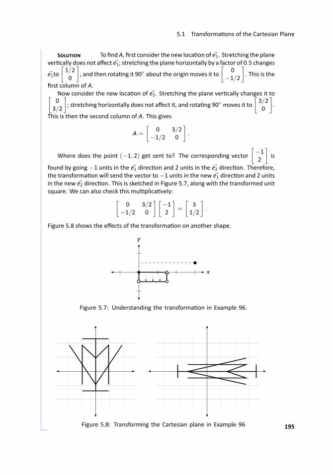
5.1 Transforma ons of the Cartesian Plane
S To findA, first consider the new loca on of e1. Stretching the planever cally does not affect e1; stretching the plane horizontally by a factor of 0.5 changes
e1to[1/20
], and then rota ng it 90◦ about the origin moves it to
[0
−1/2
]. This is the
first column of A.Now consider the new loca on of e2. Stretching the plane ver cally changes it to[0
3/2
]; stretching horizontally does not affect it, and rota ng 90◦ moves it to
[3/20
].
This is then the second column of A. This gives
A =
[0 3/2
−1/2 0
].
Where does the point (−1, 2) get sent to? The corresponding vector[−12
]is
found by going −1 units in the e1 direc on and 2 units in the e2 direc on. Therefore,the transforma on will send the vector to−1 units in the new e1 direc on and 2 unitsin the new e2 direc on. This is sketched in Figure 5.7, along with the transformed unitsquare. We can also check this mul plica vely:[
0 3/2−1/2 0
] [−12
]=
[3
1/2
].
Figure 5.8 shows the effects of the transforma on on another shape.
.. x.
y
....
..Figure 5.7: Understanding the transforma on in Example 96.
.
..Figure 5.8: Transforming the Cartesian plane in Example 96... 195
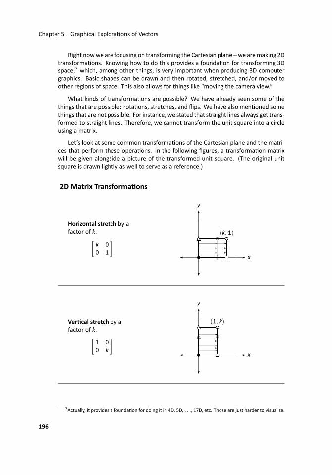
Chapter 5 Graphical Explora ons of Vectors
Right nowwe are focusing on transforming the Cartesian plane –we aremaking 2Dtransforma ons. Knowing how to do this provides a founda on for transforming 3Dspace,7 which, among other things, is very important when producing 3D computergraphics. Basic shapes can be drawn and then rotated, stretched, and/or moved toother regions of space. This also allows for things like “moving the camera view.”
What kinds of transforma ons are possible? We have already seen some of thethings that are possible: rota ons, stretches, and flips. We have also men oned somethings that are not possible. For instance, we stated that straight lines always get trans-formed to straight lines. Therefore, we cannot transform the unit square into a circleusing a matrix.
Let’s look at some common transforma ons of the Cartesian plane and the matri-ces that perform these opera ons. In the following figures, a transforma on matrixwill be given alongside a picture of the transformed unit square. (The original unitsquare is drawn lightly as well to serve as a reference.)
2D Matrix Transforma ons
Horizontal stretch by afactor of k.[
k 00 1
].. x.
y
.........
(k, 1)
Ver cal stretch by afactor of k.[
1 00 k
].. x.
y
.........
(1, k)
7Actually, it provides a founda on for doing it in 4D, 5D, . . ., 17D, etc. Those are just harder to visualize.
196
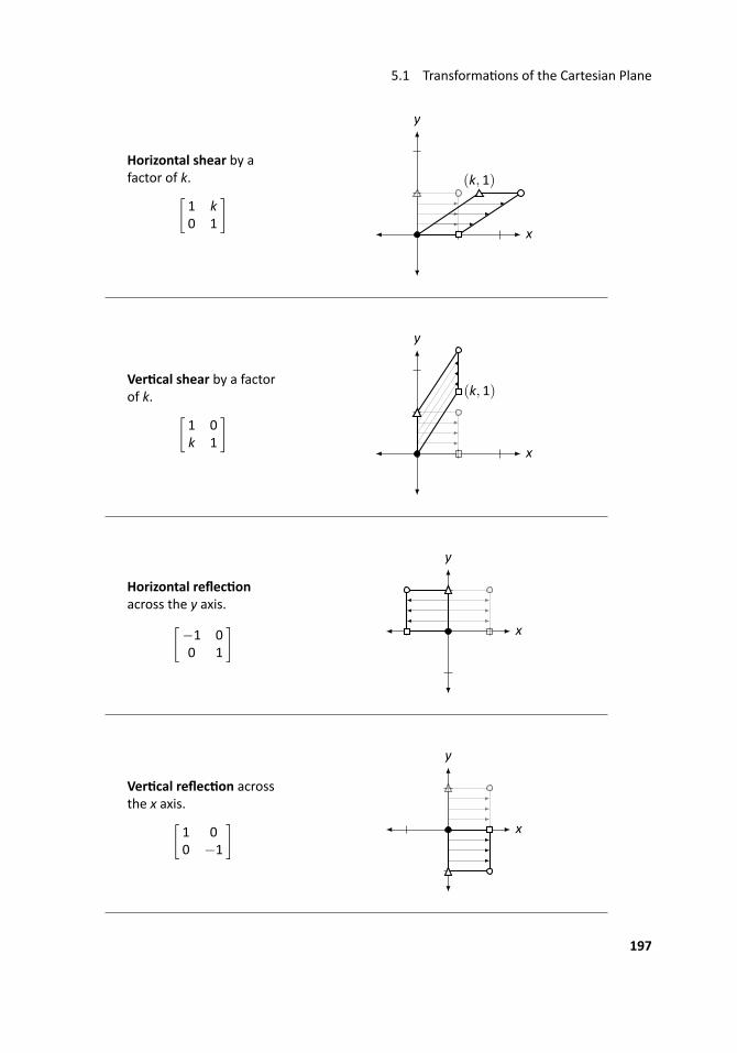
5.1 Transforma ons of the Cartesian Plane
Horizontal shear by afactor of k.[
1 k0 1
].. x.
y
.........
(k, 1)
Ver cal shear by a factorof k. [
1 0k 1
].. x.
y
.........
(k, 1)
Horizontal reflec onacross the y axis.[
−1 00 1
] .. x.
y
........
Ver cal reflec on acrossthe x axis.[
1 00 −1
] .. x.
y
........
197
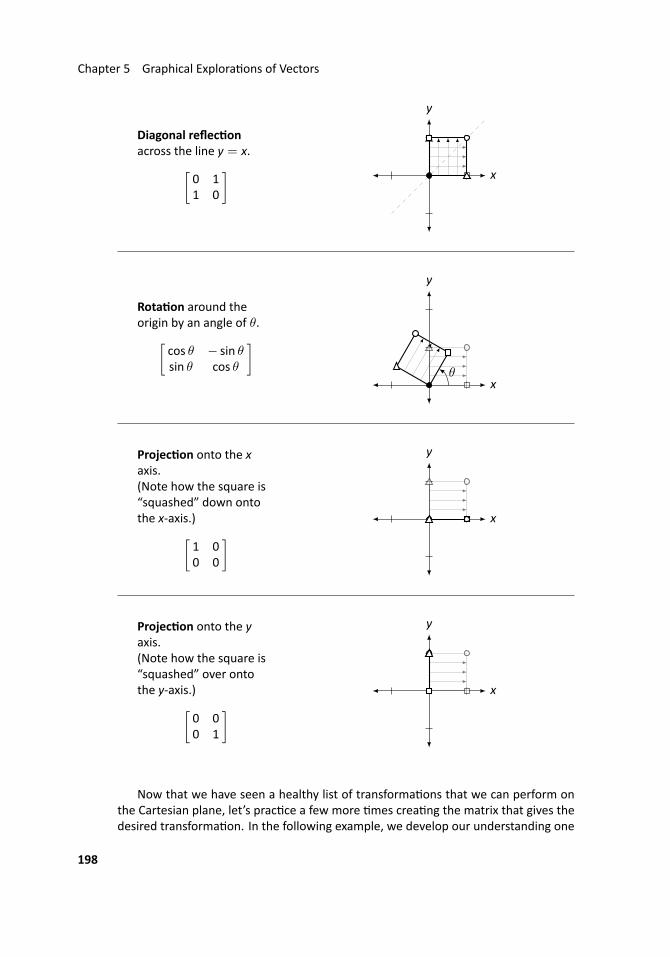
Chapter 5 Graphical Explora ons of Vectors
Diagonal reflec onacross the line y = x.[
0 11 0
] .. x.
y
........
Rota on around theorigin by an angle of θ.[
cos θ − sin θsin θ cos θ
].. x.
y
.........θ
Projec on onto the xaxis.(Note how the square is“squashed” down ontothe x-axis.)[
1 00 0
] .. x.
y
........
Projec on onto the yaxis.(Note how the square is“squashed” over ontothe y-axis.)[
0 00 1
] .. x.
y
........
Now that we have seen a healthy list of transforma ons that we can perform onthe Cartesian plane, let’s prac ce a few more mes crea ng the matrix that gives thedesired transforma on. In the following example, we develop our understanding one
198
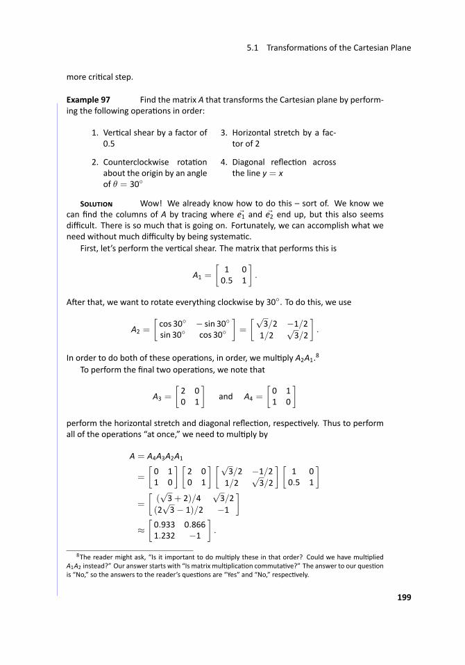
5.1 Transforma ons of the Cartesian Plane
more cri cal step.
.. Example 97 ..Find the matrix A that transforms the Cartesian plane by perform-ing the following opera ons in order:
1. Ver cal shear by a factor of0.5
2. Counterclockwise rota onabout the origin by an angleof θ = 30◦
3. Horizontal stretch by a fac-tor of 2
4. Diagonal reflec on acrossthe line y = x
S Wow! We already know how to do this – sort of. We know wecan find the columns of A by tracing where e1 and e2 end up, but this also seemsdifficult. There is so much that is going on. Fortunately, we can accomplish what weneed without much difficulty by being systema c.
First, let’s perform the ver cal shear. The matrix that performs this is
A1 =
[1 00.5 1
].
A er that, we want to rotate everything clockwise by 30◦. To do this, we use
A2 =
[cos 30◦ − sin 30◦
sin 30◦ cos 30◦
]=
[√3/2 −1/21/2
√3/2
].
In order to do both of these opera ons, in order, we mul ply A2A1.8
To perform the final two opera ons, we note that
A3 =
[2 00 1
]and A4 =
[0 11 0
]perform the horizontal stretch and diagonal reflec on, respec vely. Thus to performall of the opera ons “at once,” we need to mul ply by
A = A4A3A2A1
=
[0 11 0
] [2 00 1
] [√3/2 −1/21/2
√3/2
] [1 00.5 1
]=
[(√3+ 2)/4
√3/2
(2√3− 1)/2 −1
]≈
[0.933 0.8661.232 −1
].
8The reader might ask, “Is it important to do mul ply these in that order? Could we have mul pliedA1A2 instead?” Our answer starts with “Is matrix mul plica on commuta ve?” The answer to our ques onis “No,” so the answers to the reader’s ques ons are “Yes” and “No,” respec vely.
199
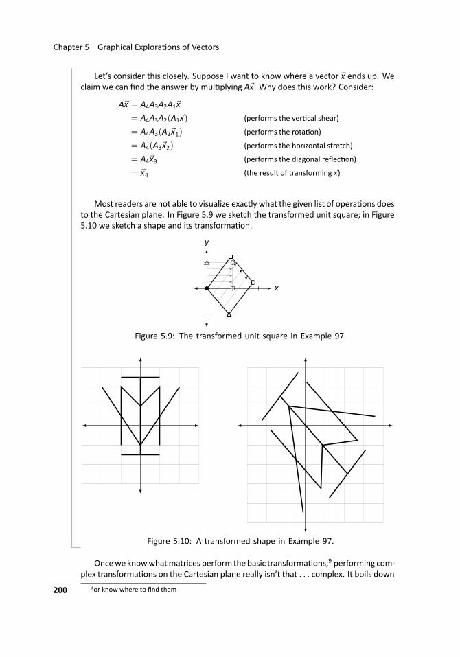
Chapter 5 Graphical Explora ons of Vectors
Let’s consider this closely. Suppose I want to know where a vector x ends up. Weclaim we can find the answer by mul plying Ax. Why does this work? Consider:
Ax = A4A3A2A1x
= A4A3A2(A1x) (performs the ver cal shear)
= A4A3(A2x1) (performs the rota on)
= A4(A3x2) (performs the horizontal stretch)
= A4x3 (performs the diagonal reflec on)
= x4 (the result of transforming x)
Most readers are not able to visualize exactly what the given list of opera ons doesto the Cartesian plane. In Figure 5.9 we sketch the transformed unit square; in Figure5.10 we sketch a shape and its transforma on.
.. x.
y
........
..Figure 5.9: The transformed unit square in Example 97.
.
..Figure 5.10: A transformed shape in Example 97....
Onceweknowwhatmatrices perform thebasic transforma ons,9 performing com-plex transforma ons on the Cartesian plane really isn’t that . . . complex. It boils down
9or know where to find them200
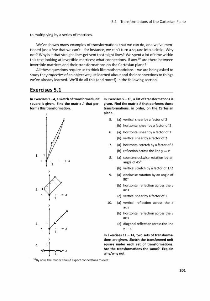
5.1 Transforma ons of the Cartesian Plane
to mul plying by a series of matrices.
We’ve shown many examples of transforma ons that we can do, and we’ve men-oned just a few that we can’t – for instance, we can’t turn a square into a circle. Why
not? Why is it that straight lines get sent to straight lines? We spent a lot of mewithinthis text looking at inver ble matrices; what connec ons, if any,10 are there betweeninver ble matrices and their transforma ons on the Cartesian plane?
All these ques ons require us to think like mathema cians – we are being asked tostudy the proper es of an object we just learned about and their connec ons to thingswe’ve already learned. We’ll do all this (and more!) in the following sec on.
Exercises 5.1In Exercises 1 – 4, a sketch of transformed unitsquare is given. Find the matrix A that per-forms this transforma on.
1... x.
y
.1
.1....
2... x.
y
.1
.1....
3... x.
y
.1
.1....
4... x.
y
.1
.1....
In Exercises 5 – 10, a list of transforma ons isgiven. Find the matrix A that performs thosetransforma ons, in order, on the Cartesianplane.
5. (a) ver cal shear by a factor of 2
(b) horizontal shear by a factor of 2
6. (a) horizontal shear by a factor of 2
(b) ver cal shear by a factor of 2
7. (a) horizontal stretch by a factor of 3
(b) reflec on across the line y = x
8. (a) counterclockwise rota on by anangle of 45◦
(b) ver cal stretch by a factor of 1/2
9. (a) clockwise rota on by an angle of90◦
(b) horizontal reflec on across the yaxis
(c) ver cal shear by a factor of 1
10. (a) ver cal reflec on across the xaxis
(b) horizontal reflec on across the yaxis
(c) diagonal reflec on across the liney = x
In Exercises 11 – 14, two sets of transforma-ons are given. Sketch the transformed unit
square under each set of transforma ons.Are the transforma ons the same? Explainwhy/why not.
10By now, the reader should expect connec ons to exist.
201
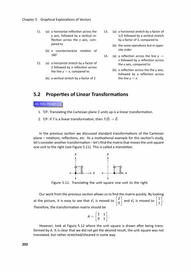
Chapter 5 Graphical Explora ons of Vectors
11. (a) a horizontal reflec on across they axis, followed by a ver cal re-flec on across the x axis, com-pared to
(b) a counterclockise rota on of180◦
12. (a) a horizontal stretch by a factor of2 followed by a reflec on acrossthe line y = x, compared to
(b) a ver cal stretch by a factor of 2
13. (a) a horizontal stretch by a factor of1/2 followed by a ver cal stretchby a factor of 3, compared to
(b) the same opera ons but in oppo-site order
14. (a) a reflec on across the line y =x followed by a reflec on acrossthe x axis, compared to
(b) a reflec on across the the y axis,followed by a reflec on acrossthe line y = x.
5.2 Proper es of Linear Transforma ons
...AS YOU READ . . .
1. T/F: Transla ng the Cartesian plane 2 units up is a linear transforma on.
2. T/F: If T is a linear transforma on, then T(0) = 0.
In the previous sec on we discussed standard transforma ons of the Cartesianplane – rota ons, reflec ons, etc. As a mo va onal example for this sec on’s study,let’s consider another transforma on – let’s find thematrix thatmoves the unit squareone unit to the right (see Figure 5.11). This is called a transla on.
.. x.
y
..... x.
y
....
..Figure 5.11: Transla ng the unit square one unit to the right.
Our work from the previous sec on allows us to find the matrix quickly. By looking
at the picture, it is easy to see that e1 is moved to[20
]and e2 is moved to
[11
].
Therefore, the transforma on matrix should be
A =
[2 10 1
].
However, look at Figure 5.12 where the unit square is drawn a er being trans-formed by A. It is clear that we did not get the desired result; the unit square was nottranslated, but rather stretched/sheared in some way.
202
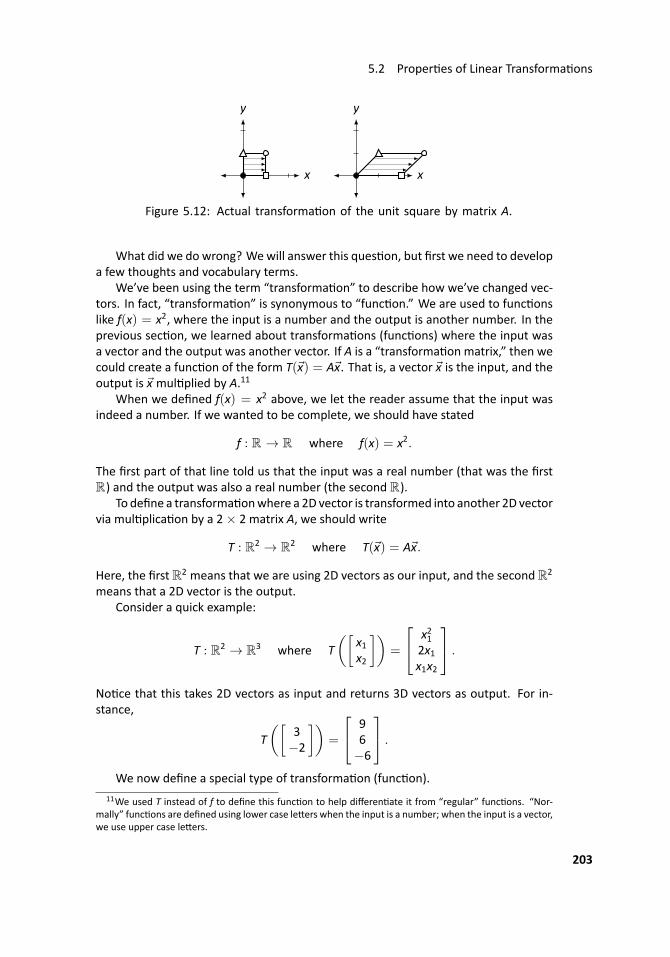
5.2 Proper es of Linear Transforma ons
.. x.
y
..... x.
y
....
..Figure 5.12: Actual transforma on of the unit square by matrix A.
What did we do wrong? Wewill answer this ques on, but first we need to developa few thoughts and vocabulary terms.
We’ve been using the term “transforma on” to describe how we’ve changed vec-tors. In fact, “transforma on” is synonymous to “func on.” We are used to func onslike f(x) = x2, where the input is a number and the output is another number. In theprevious sec on, we learned about transforma ons (func ons) where the input wasa vector and the output was another vector. If A is a “transforma on matrix,” then wecould create a func on of the form T(x) = Ax. That is, a vector x is the input, and theoutput is x mul plied by A.11
When we defined f(x) = x2 above, we let the reader assume that the input wasindeed a number. If we wanted to be complete, we should have stated
f : R → R where f(x) = x2.
The first part of that line told us that the input was a real number (that was the firstR) and the output was also a real number (the second R).
To define a transforma onwhere a 2D vector is transformed into another 2D vectorvia mul plica on by a 2× 2 matrix A, we should write
T : R2 → R2 where T(x) = Ax.
Here, the firstR2 means that we are using 2D vectors as our input, and the secondR2
means that a 2D vector is the output.Consider a quick example:
T : R2 → R3 where T([
x1x2
])=
x212x1x1x2
.
No ce that this takes 2D vectors as input and returns 3D vectors as output. For in-stance,
T([
3−2
])=
96−6
.
We now define a special type of transforma on (func on).11We used T instead of f to define this func on to help differen ate it from “regular” func ons. “Nor-
mally” func ons are defined using lower case le ers when the input is a number; when the input is a vector,we use upper case le ers.
203
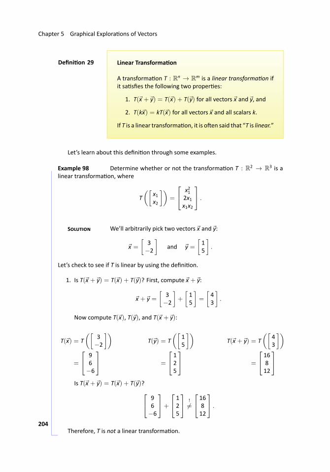
Chapter 5 Graphical Explora ons of Vectors
..Defini on 29
.
.Linear Transforma on
A transforma on T : Rn → Rm is a linear transforma on ifit sa sfies the following two proper es:
1. T(x + y) = T(x) + T(y) for all vectors x and y, and
2. T(kx) = kT(x) for all vectors x and all scalars k.
If T is a linear transforma on, it is o en said that “T is linear.”
Let’s learn about this defini on through some examples.
.. Example 98 Determine whether or not the transforma on T : R2 → R3 is alinear transforma on, where
T([
x1x2
])=
x212x1x1x2
.
S We’ll arbitrarily pick two vectors x and y:
x =
[3−2
]and y =
[15
].
Let’s check to see if T is linear by using the defini on.
1. Is T(x + y) = T(x) + T(y)? First, compute x + y:
x + y =[
3−2
]+
[15
]=
[43
].
Now compute T(x), T(y), and T(x + y):
T(x) = T([
3−2
])
=
96−6
T(y) = T
([15
])
=
125
T(x + y) = T
([43
])
=
16812
Is T(x + y) = T(x) + T(y)? 9
6−6
+
125
!
=
16812
.
Therefore, T is not a linear transforma on. ..204
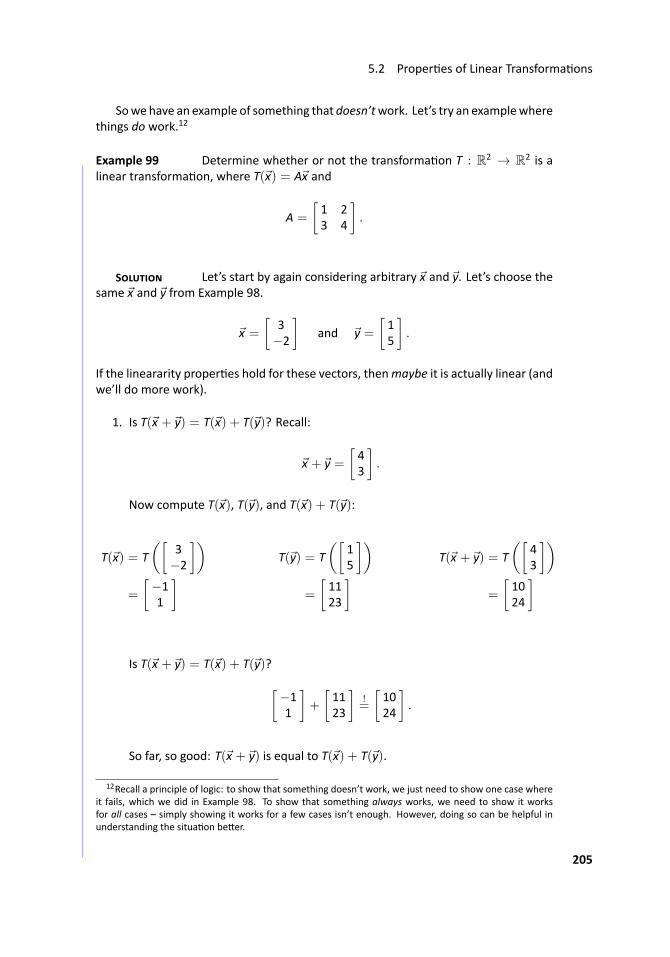
5.2 Proper es of Linear Transforma ons
Sowehave an example of something that doesn’twork. Let’s try an examplewherethings do work.12
.. Example 99 ..Determine whether or not the transforma on T : R2 → R2 is alinear transforma on, where T(x) = Ax and
A =
[1 23 4
].
S Let’s start by again considering arbitrary x and y. Let’s choose thesame x and y from Example 98.
x =
[3−2
]and y =
[15
].
If the lineararity proper es hold for these vectors, thenmaybe it is actually linear (andwe’ll do more work).
1. Is T(x + y) = T(x) + T(y)? Recall:
x + y =[43
].
Now compute T(x), T(y), and T(x) + T(y):
T(x) = T([
3−2
])=
[−11
] T(y) = T([
15
])=
[1123
] T(x + y) = T([
43
])=
[1024
]
Is T(x + y) = T(x) + T(y)?[−11
]+
[1123
]!=
[1024
].
So far, so good: T(x + y) is equal to T(x) + T(y).
12Recall a principle of logic: to show that something doesn’t work, we just need to show one case whereit fails, which we did in Example 98. To show that something always works, we need to show it worksfor all cases – simply showing it works for a few cases isn’t enough. However, doing so can be helpful inunderstanding the situa on be er.
205
Chapter 5 Graphical Explora ons of Vectors
2. Is T(kx) = kT(x)? Let’s arbitrarily pick k = 7, and use x as before.
T(7x) = T([
21−14
])=
[−77
]= 7
[−11
]= 7 · T(x) !
So far it seems that T is indeed linear, for it worked in one example with arbitrarilychosen vectors and scalar. Now we need to try to show it is always true.
Consider T(x + y). By the defini on of T, we have
T(x + y) = A(x + y).
By Theorem 3, part 2 (on page 62) we state that the Distribu ve Property holds formatrix mul plica on.13 So A(x + y) = Ax + Ay. Recognize now that this last part isjust T(x) + T(y)! We repeat the above steps, all together:
T(x + y) = A(x + y) (by the defini on of T in this example)
= Ax + Ay (by the Distribu ve Property)
= T(x) + T(y) (again, by the defini on of T)
Therefore, no ma er what x and y are chosen, T(x + y) = T(x) + T(y). Thus the firstpart of the lineararity defini on is sa sfied.
The second part is sa sfied in a similar fashion. Let k be a scalar, and consider:
T(kx) = A(kx) (by the defini on of T is this example)
= kAx (by Theorem 3 part 3)
= kT(x) (again, by the defini on of T)
Since T sa sfies both parts of the defini on, we conclude that T is a linear trans-forma on. ...
Wehave seen twoexamples of transforma ons so far, onewhichwas not linear andone that was. One might wonder “Why is linearity important?”, which we’ll addressshortly.
First, consider how we proved the transforma on in Example 99 was linear. Wedefined T by matrix mul plica on, that is, T(x) = Ax. We proved T was linear usingproper es of matrix mul plica on –we never considered the specific values of A! Thatis, we didn’t just choose a good matrix for T; any matrix A would have worked. This
13Recall that a vector is just a special type of matrix, so this theorem applies to matrix–vector mul plica-on as well.
206
5.2 Proper es of Linear Transforma ons
leads us to an important theorem. The first part we have essen ally just proved; thesecond part we won’t prove, although its truth is very powerful.
..Theorem 21
.
.Matrices and Linear Transforma ons
1. Define T : Rn → Rm by T(x) = Ax, where A is anm× nmatrix. Then T is a linear transforma on.
2. Let T : Rn → Rm be any linear transforma on. Thenthere exists an uniquem×nmatrixA such that T(x) =Ax.
The second part of the theorem says that all linear transforma ons can be de-scribed using matrix mul plica on. Given any linear transforma on, there is a matrixthat completely defines that transforma on. This importantmatrix gets its own name.
..Defini on 30
.
.Standard Matrix of a Linear Transforma on
Let T : Rn → Rm be a linear transforma on. By Theorem21, there is a matrix A such that T(x) = Ax. This matrix Ais called the standard matrix of the linear transforma on T,and is denoted [ T ].a
aThe matrix–like brackets around T suggest that the standard matrix Ais a matrix “with T inside.”
While exploring all of the ramifica ons of Theorem 21 is outside the scope of thistext, let it suffice to say that since 1) linear transforma ons are very, very importantin economics, science, engineering and mathema cs, and 2) the theory of matrices iswell developed and easy to implement by hand and on computers, then 3) it is greatnews that these two concepts go hand in hand.
We have already used the second part of this theorem in a small way. In the pre-vious sec on we looked at transforma ons graphically and found the matrices thatproduced them. At the me, we didn’t realize that these transforma ons were linear,but indeed they were.
This brings us back to the mo va ng example with which we started this sec on.We tried to find the matrix that translated the unit square one unit to the right. Oura empt failed, and we have yet to determine why. Given our link between matricesand linear transforma ons, the answer is likely “the transla on transforma on is nota linear transforma on.” While that is a true statement, it doesn’t really explain thingsall that well. Is there some way we could have recognized that this transforma on
207
Chapter 5 Graphical Explora ons of Vectors
wasn’t linear?14
Yes, there is. Consider the second part of the linear transforma on defini on. Itstates that T(kx) = kT(x) for all scalars k. If we let k = 0, we have T(0x) = 0 · T(x), ormore simply, T(0) = 0. That is, if T is to be a linear transforma on, it must send thezero vector to the zero vector.
This is a quick way to see that the transla on transforma on fails to be linear. Byshi ing the unit square to the right one unit, the corner at the point (0, 0)was sent tothe point (1, 0), i.e.,
the vector[00
]was sent to the vector
[10
].
This property rela ng to 0 is important, so we highlight it here.
..Key Idea 15
.
.Linear Transforma ons and 0
Let T : Rn → Rm be a linear transforma on. Then:
T(0n) = 0m.
That is, the zero vector in Rn gets sent to the zero vector inRm.
The interested reader may wish to read the footnote below.15
The Standard Matrix of a Linear Transforma on
It is o en the case that while one can describe a linear transforma on, one doesn’tknow what matrix performs that transforma on (i.e., one doesn’t know the standardmatrix of that linear transforma on). How do we systema cally find it? We’ll need anew defini on.
..Defini on 31
.
.Standard Unit Vectors
In Rn, the standard unit vectors ei are the vectors with a 1in the ith entry and 0s everywhere else.
14That is, apart from applying the defini on directly?15The idea that linear transforma ons “send zero to zero” has an interes ng rela on to terminology. The
reader is likely familiar with func ons like f(x) = 2x+ 3 and would likely refer to this as a “linear func on.”However, f(0) = 0, so f is not “linear” by our new defini on of linear. We erroneously call f “linear” sinceits graph produces a line, though we should be careful to instead state that “the graph of f is a line.”
208
5.2 Proper es of Linear Transforma ons
We’ve already seen these vectors in the previous sec on. In R2, we iden fied
e1 =[10
]and e2 =
[01
].
In R4, there are 4 standard unit vectors:
e1 =
1000
, e2 =
0100
, e3 =
0010
, and e4 =
0001
.
How do these vectors help us find the standard matrix of a linear transforma on?Recall again our work in the previous sec on. There, we prac ced looking at the trans-formed unit square and deducing the standard transforma on matrix A. We did thisby making the first column of A the vector where e1 ended up and making the secondcolumn of A the vector where e2 ended up. One could represent this with:
A =[T(e1) T(e2)
]= [ T ].
That is, T(e1) is the vector where e1 ends up, and T(e2) is the vector where e2 ends up.The same holds true in general. Given a linear transforma on T : Rn → Rm, the
standard matrix of T is the matrix whose ith column is the vector where ei ends up.While we won’t prove this is true, it is, and it is very useful. Therefore we’ll state itagain as a theorem.
..Theorem 22
.
.The Standard Matrix of a Linear Transforma on
Let T : Rn → Rm be a linear transforma on. Then [ T ] is them× nmatrix:
[ T ] =[T(e1) T(e2) · · · T(en)
].
Let’s prac ce this theorem in an example.
.. Example 100 ..Define T : R3 → R4 to be the linear transforma on where
T
x1x2x3
=
x1 + x23x1 − x32x2 + 5x3
4x1 + 3x2 + 2x3
.
Find [ T ].
209
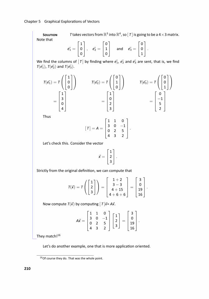
Chapter 5 Graphical Explora ons of Vectors
S T takes vectors fromR3 intoR4, so [ T ] is going to be a 4×3matrix.Note that
e1 =
100
, e2 =
010
and e3 =
001
.
We find the columns of [ T ] by finding where e1, e2 and e3 are sent, that is, we findT(e1), T(e2) and T(e3).
T(e1) = T
100
=
1304
T(e2) = T
010
=
1023
T(e3) = T
001
=
0−152
Thus
[ T ] = A =
1 1 03 0 −10 2 54 3 2
.
Let’s check this. Consider the vector
x =
123
.
Strictly from the original defini on, we can compute that
T(x) = T
123
=
1+ 23− 34+ 15
4+ 6+ 6
=
301916
.
Now compute T(x) by compu ng [ T ]x= Ax.
Ax =
1 1 03 0 −10 2 54 3 2
123
=
301916
.
They match!16 ...
Let’s do another example, one that is more applica on oriented.
16Of course they do. That was the whole point.
210
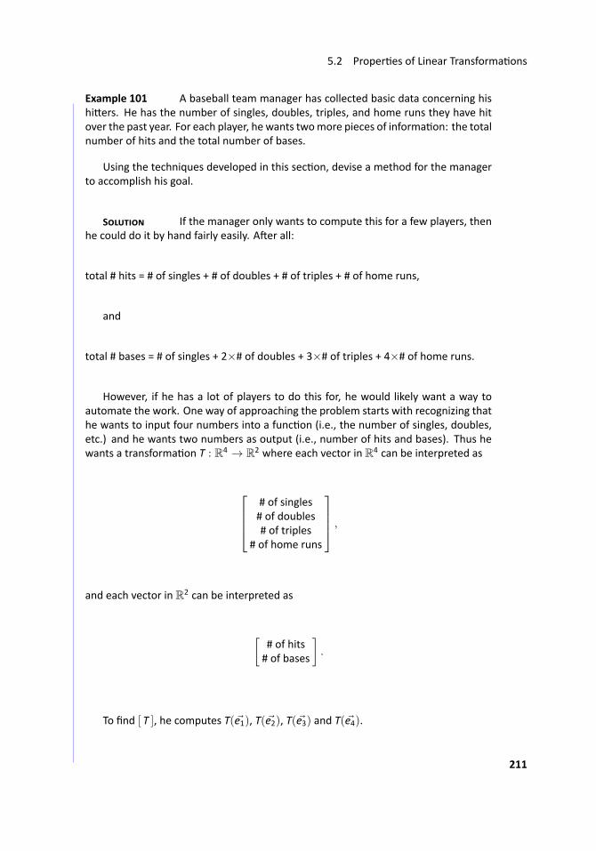
5.2 Proper es of Linear Transforma ons
.. Example 101 ..A baseball team manager has collected basic data concerning hishi ers. He has the number of singles, doubles, triples, and home runs they have hitover the past year. For each player, he wants twomore pieces of informa on: the totalnumber of hits and the total number of bases.
Using the techniques developed in this sec on, devise a method for the managerto accomplish his goal.
S If the manager only wants to compute this for a few players, thenhe could do it by hand fairly easily. A er all:
total # hits = # of singles + # of doubles + # of triples + # of home runs,
and
total # bases = # of singles + 2×# of doubles + 3×# of triples + 4×# of home runs.
However, if he has a lot of players to do this for, he would likely want a way toautomate the work. One way of approaching the problem starts with recognizing thathe wants to input four numbers into a func on (i.e., the number of singles, doubles,etc.) and he wants two numbers as output (i.e., number of hits and bases). Thus hewants a transforma on T : R4 → R2 where each vector in R4 can be interpreted as
# of singles# of doubles# of triples
# of home runs
,
and each vector in R2 can be interpreted as
[# of hits# of bases
].
To find [ T ], he computes T(e1), T(e2), T(e3) and T(e4).
211
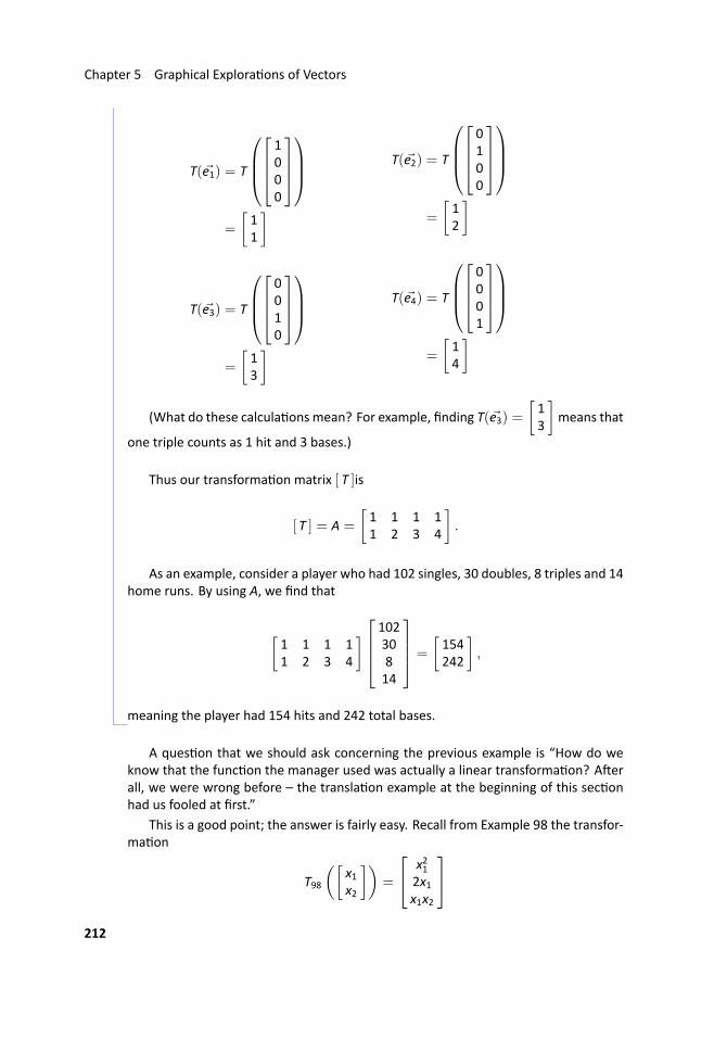
Chapter 5 Graphical Explora ons of Vectors
T(e1) = T
1000
=
[11
]
T(e3) = T
0010
=
[13
]
T(e2) = T
0100
=
[12
]
T(e4) = T
0001
=
[14
]
(What do these calcula ons mean? For example, finding T(e3) =[13
]means that
one triple counts as 1 hit and 3 bases.)
Thus our transforma on matrix [ T ]is
[ T ] = A =
[1 1 1 11 2 3 4
].
As an example, consider a player who had 102 singles, 30 doubles, 8 triples and 14home runs. By using A, we find that
[1 1 1 11 2 3 4
]10230814
=
[154242
],
meaning the player had 154 hits and 242 total bases. ...
A ques on that we should ask concerning the previous example is “How do weknow that the func on the manager used was actually a linear transforma on? A erall, we were wrong before – the transla on example at the beginning of this sec onhad us fooled at first.”
This is a good point; the answer is fairly easy. Recall from Example 98 the transfor-ma on
T98
([x1x2
])=
x212x1x1x2
212
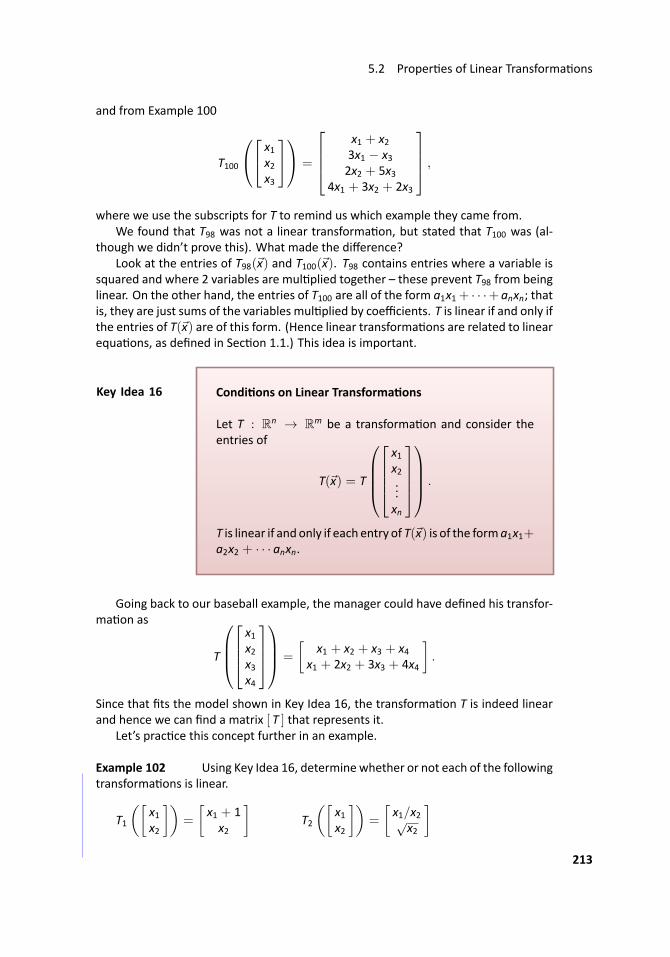
5.2 Proper es of Linear Transforma ons
and from Example 100
T100
x1x2x3
=
x1 + x23x1 − x32x2 + 5x3
4x1 + 3x2 + 2x3
,
where we use the subscripts for T to remind us which example they came from.We found that T98 was not a linear transforma on, but stated that T100 was (al-
though we didn’t prove this). What made the difference?Look at the entries of T98(x) and T100(x). T98 contains entries where a variable is
squared and where 2 variables are mul plied together – these prevent T98 from beinglinear. On the other hand, the entries of T100 are all of the form a1x1+ · · ·+ anxn; thatis, they are just sums of the variables mul plied by coefficients. T is linear if and only ifthe entries of T(x) are of this form. (Hence linear transforma ons are related to linearequa ons, as defined in Sec on 1.1.) This idea is important.
..Key Idea 16
.
.Condi ons on Linear Transforma ons
Let T : Rn → Rm be a transforma on and consider theentries of
T(x) = T
x1x2...xn
.
T is linear if andonly if each entry of T(x) is of the forma1x1+a2x2 + · · · anxn.
Going back to our baseball example, the manager could have defined his transfor-ma on as
T
x1x2x3x4
=
[x1 + x2 + x3 + x4
x1 + 2x2 + 3x3 + 4x4
].
Since that fits the model shown in Key Idea 16, the transforma on T is indeed linearand hence we can find a matrix [ T ] that represents it.
Let’s prac ce this concept further in an example.
.. Example 102 ..Using Key Idea 16, determinewhether or not each of the followingtransforma ons is linear.
T1
([x1x2
])=
[x1 + 1x2
]T2
([x1x2
])=
[x1/x2√
x2
]213
Chapter 5 Graphical Explora ons of Vectors
T3
([x1x2
])=
[√7x1 − x2πx2
]S T1 is not linear! This may come as a surprise, but we are not al-
lowed to add constants to the variables. By thinking about this, we can see that thistransforma on is trying to accomplish the transla on that got us started in this sec on– it adds 1 to all the x values and leaves the y values alone, shi ing everything to theright one unit. However, this is not linear; again, no ce how 0 does not get mappedto 0.
T2 is also not linear. We cannot divide variables, nor can we put variabless in-side the square root func on (among other other things; again, see Sec on 1.1). Thismeans that the baseball manager would not be able to use matrices to compute aba ng average, which is (number of hits)/(number of at bats).
T3 is linear. Recall that√7 and π are just numbers, just coefficients. ...
We’vemen oned before that we can draw vectors other than 2D vectors, althoughthe more dimensions one adds, the harder it gets to understand. In the next sec onwe’ll learn about graphing vectors in 3D – that is, how to draw on paper or a computerscreen a 3D vector.
Exercises 5.2In Exercises 1 – 5, a transforma on T is given.Determine whether or not T is linear; if not,state why not.
1. T([
x1x2
])=
[x1 + x23x1 − x2
]2. T
([x1x2
])=
[x1 + x22x1 − x2
]3. T
([x1x2
])=
[x1 + 1x2 + 1
]4. T
([x1x2
])=
[11
]5. T
([x1x2
])=
[00
]In Exercises 6 – 11, a linear transforma on Tis given. Find [ T ].
6. T([
x1x2
])=
[x1 + x2x1 − x2
]
7. T([
x1x2
])=
x1 + 2x23x1 − 5x2
2x2
8. T
x1x2x3
=
x1 + 2x2 − 3x3
0x1 + 4x35x2 + x3
9. T
x1x2x3
=
x1 + 3x3x1 − x3x1 + x3
10. T
([x1x2
])=
[00
]
11. T
x1x2x3x4
=
[x1 + 2x2 + 3x3 + 4x4
]
214
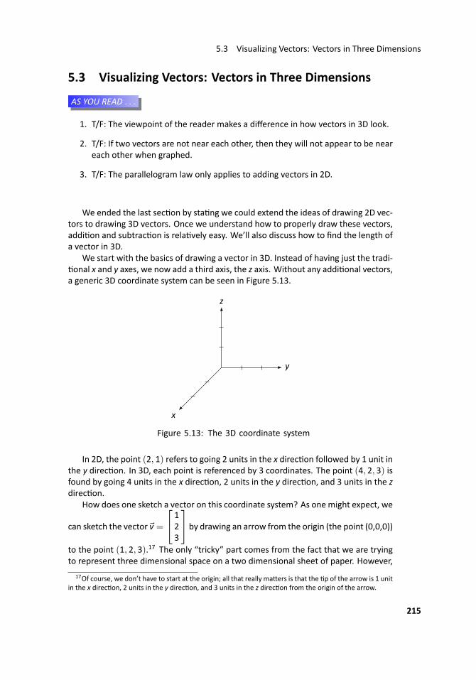
5.3 Visualizing Vectors: Vectors in Three Dimensions
5.3 Visualizing Vectors: Vectors in Three Dimensions
...AS YOU READ . . .
1. T/F: The viewpoint of the reader makes a difference in how vectors in 3D look.
2. T/F: If two vectors are not near each other, then they will not appear to be neareach other when graphed.
3. T/F: The parallelogram law only applies to adding vectors in 2D.
We ended the last sec on by sta ng we could extend the ideas of drawing 2D vec-tors to drawing 3D vectors. Once we understand how to properly draw these vectors,addi on and subtrac on is rela vely easy. We’ll also discuss how to find the length ofa vector in 3D.
We start with the basics of drawing a vector in 3D. Instead of having just the tradi-onal x and y axes, we now add a third axis, the z axis. Without any addi onal vectors,
a generic 3D coordinate system can be seen in Figure 5.13.
..
x
. y.
z
..Figure 5.13: The 3D coordinate system
In 2D, the point (2, 1) refers to going 2 units in the x direc on followed by 1 unit inthe y direc on. In 3D, each point is referenced by 3 coordinates. The point (4, 2, 3) isfound by going 4 units in the x direc on, 2 units in the y direc on, and 3 units in the zdirec on.
How does one sketch a vector on this coordinate system? As onemight expect, we
can sketch the vector v =
123
by drawing an arrow from the origin (the point (0,0,0))
to the point (1, 2, 3).17 The only “tricky” part comes from the fact that we are tryingto represent three dimensional space on a two dimensional sheet of paper. However,
17Of course, we don’t have to start at the origin; all that really ma ers is that the p of the arrow is 1 unitin the x direc on, 2 units in the y direc on, and 3 units in the z direc on from the origin of the arrow.
215
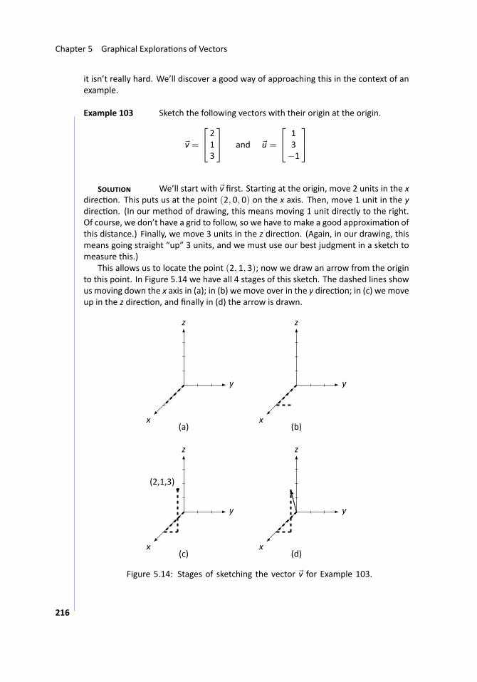
Chapter 5 Graphical Explora ons of Vectors
it isn’t really hard. We’ll discover a good way of approaching this in the context of anexample.
.. Example 103 ..Sketch the following vectors with their origin at the origin.
v =
213
and u =
13−1
S We’ll start with v first. Star ng at the origin, move 2 units in the xdirec on. This puts us at the point (2, 0, 0) on the x axis. Then, move 1 unit in the ydirec on. (In our method of drawing, this means moving 1 unit directly to the right.Of course, we don’t have a grid to follow, so we have to make a good approxima on ofthis distance.) Finally, we move 3 units in the z direc on. (Again, in our drawing, thismeans going straight “up” 3 units, and we must use our best judgment in a sketch tomeasure this.)
This allows us to locate the point (2, 1, 3); now we draw an arrow from the originto this point. In Figure 5.14 we have all 4 stages of this sketch. The dashed lines showus moving down the x axis in (a); in (b) we move over in the y direc on; in (c) we moveup in the z direc on, and finally in (d) the arrow is drawn.
..
x
. y.
z
.
(a)
.
x
. y.
z
.
(b)
.
x
.
y
.
z
.
(2,1,3)
.
(c)
.
x
.
y
.
z
.
(d)
..Figure 5.14: Stages of sketching the vector v for Example 103.
216
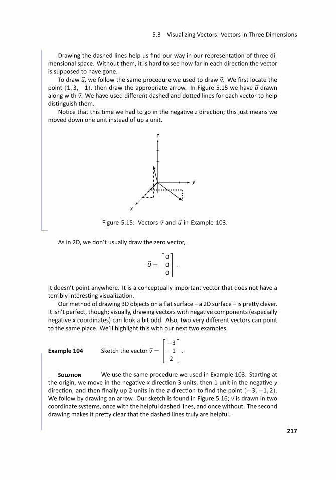
5.3 Visualizing Vectors: Vectors in Three Dimensions
Drawing the dashed lines help us find our way in our representa on of three di-mensional space. Without them, it is hard to see how far in each direc on the vectoris supposed to have gone.
To draw u, we follow the same procedure we used to draw v. We first locate thepoint (1, 3,−1), then draw the appropriate arrow. In Figure 5.15 we have u drawnalong with v. We have used different dashed and do ed lines for each vector to helpdis nguish them.
No ce that this me we had to go in the nega ve z direc on; this just means wemoved down one unit instead of up a unit.
..
x
. y.
z
..Figure 5.15: Vectors v and u in Example 103....
As in 2D, we don’t usually draw the zero vector,
0 =
000
.
It doesn’t point anywhere. It is a conceptually important vector that does not have aterribly interes ng visualiza on.
Ourmethod of drawing 3D objects on a flat surface – a 2D surface – is pre y clever.It isn’t perfect, though; visually, drawing vectors with nega ve components (especiallynega ve x coordinates) can look a bit odd. Also, two very different vectors can pointto the same place. We’ll highlight this with our next two examples.
.. Example 104 ..Sketch the vector v =
−3−12
.S We use the same procedure we used in Example 103. Star ng at
the origin, we move in the nega ve x direc on 3 units, then 1 unit in the nega ve ydirec on, and then finally up 2 units in the z direc on to find the point (−3,−1, 2).We follow by drawing an arrow. Our sketch is found in Figure 5.16; v is drawn in twocoordinate systems, once with the helpful dashed lines, and once without. The seconddrawing makes it pre y clear that the dashed lines truly are helpful.
217
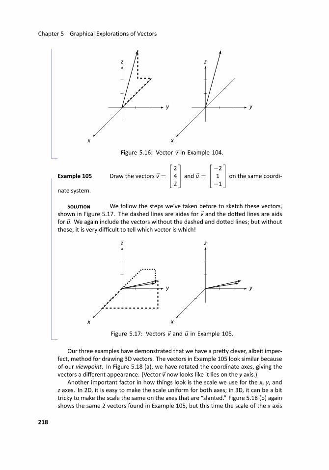
Chapter 5 Graphical Explora ons of Vectors
..
x
. y.
z
.
x
. y.
z
..Figure 5.16: Vector v in Example 104....
.. Example 105 Draw the vectors v =
242
and u =
−21−1
on the same coordi-
nate system.
S We follow the steps we’ve taken before to sketch these vectors,shown in Figure 5.17. The dashed lines are aides for v and the do ed lines are aidsfor u. We again include the vectors without the dashed and do ed lines; but withoutthese, it is very difficult to tell which vector is which!
..
x
. y.
z
.
x
. y.
z
..Figure 5.17: Vectors v and u in Example 105...
Our three examples have demonstrated that we have a pre y clever, albeit imper-fect, method for drawing 3D vectors. The vectors in Example 105 look similar becauseof our viewpoint. In Figure 5.18 (a), we have rotated the coordinate axes, giving thevectors a different appearance. (Vector v now looks like it lies on the y axis.)
Another important factor in how things look is the scale we use for the x, y, andz axes. In 2D, it is easy to make the scale uniform for both axes; in 3D, it can be a bittricky to make the scale the same on the axes that are “slanted.” Figure 5.18 (b) againshows the same 2 vectors found in Example 105, but this me the scale of the x axis
218
5.3 Visualizing Vectors: Vectors in Three Dimensions
is a bit different. The end result is that again the vectors appear a bit different thanthey did before. These facts do not necessarily pose a big problem; we must merelybe aware of these facts and not make judgments about 3D objects based on one 2Dimage.18
..
x
.
y
.
z
.
(a)
..
x
. y.
z
.
(b)
..Figure 5.18: Vectors v and u in Example 105 witha different viewpoint (a) and x axis scale (b).
We now inves gate proper es of vector arithme c: what happens (i.e., how dowe draw) when we add 3D vectors and mul ply by a scalar? How do we compute thelength of a 3D vector?
Vector Addi on and Subtrac on
In 2D, we saw that we could add vectors together graphically using the Parallelo-gram Law. Does the same apply for adding vectors in 3D?We inves gate in an example.
.. Example 106 ..Let v =
213
and u =
13−1
. Sketch v+ u.
S We sketched each of these vectors previously in Example 103. We
sketch them, along with v+ u =
342
, in Figure 5.19 (a). (We use loosely dashed lines
for v+ u.)
18The human brain uses both eyes to convey 3D, or depth, informa on. With one eye closed (or missing),we can have a very hard me with “depth percep on.” Two objects that are far apart can seem very closetogether. A simple example of this problem is this: close one eye, and place your index finger about a footabove this text, directly above this WORD. See if you were correct by dropping your finger straight down.Did you actually hit the proper spot? Try it again with both eyes, and you should see a no cable differencein your accuracy.
Looking at 3D objects on paper is a bit like viewing the world with one eye closed.
219
Chapter 5 Graphical Explora ons of Vectors
Does the Parallelogram Law s ll hold? In Figure 5.19 (b), we draw addi onal rep-resenta ons of v and u to form a parallelogram (without all the do ed lines), whichseems to affirm the fact that the Parallelogram Law does indeed hold.
..
x
. y.
z
.
(b)
.
x
. y.
z
.
(b)
..Figure 5.19: Vectors v, u, and v + u Example 106.
...
We also learned that in 2D, we could subtract vectors by drawing a vector from thep of one vector to the other.19 Does this also work in 3D?We’ll inves gate again with
an example, using the familiar vectors v and u from before.
.. Example 107 ..Let v =
213
and u =
13−1
. Sketch v− u.
S It is simple to compute that v − u =
1−24
. All three of these
vectors are sketched in Figure 5.20 (a), where again v is guided by the dashed, u by thedo ed, and v− u by the loosely dashed lines.
Does the 2D subtrac on rule s ll hold? That is, can we draw v − u by drawing anarrow from the p of u to the p of v? In Figure 5.20 (b), we translate the drawing ofv− u to the p of u, and sure enough, it looks like it works. (And in fact, it really does.)
19Recall that it is important which vector we used for the origin and which was used for the p.
220
5.3 Visualizing Vectors: Vectors in Three Dimensions
..
x
. y.
z
.
(a)
.
x
. y.
z
.
(b)
..Figure 5.20: Vectors v, u, and v − u from Example 107.
...
The previous two examples highlight the fact that even in 3D, we can sketch vec-tors without explicitly knowing what they are. We prac ce this one more me in thefollowing example.
.. Example 108 ..Vectors v and u are drawn in Figure 5.21. Using this drawing, sketchthe vectors v+ u and v− u.
..
x
. y.
z
.
v
.
u
..Figure 5.21: Vectors v and u for Example 108.
S Using the Parallelogram Law, we draw v + u by first drawing a grayversion of u coming from the p of v; v+ u is drawn dashed in Figure 5.22.
To draw v− u, we draw a do ed arrow from the p of uto the p of v.
221
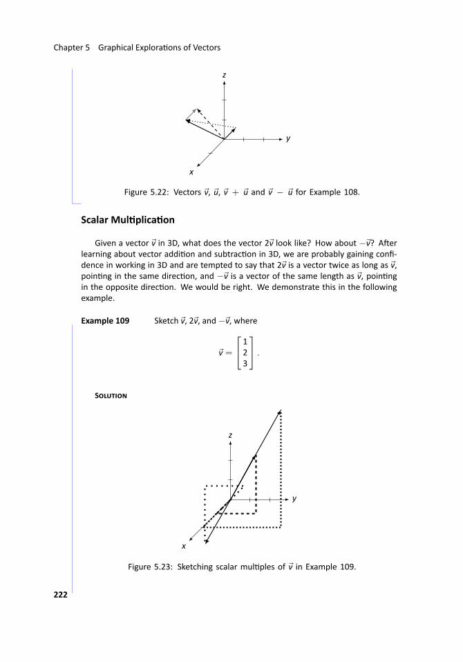
Chapter 5 Graphical Explora ons of Vectors
..
x
. y.
z
..Figure 5.22: Vectors v, u, v + u and v − u for Example 108....
Scalar Mul plica on
Given a vector v in 3D, what does the vector 2v look like? How about −v? A erlearning about vector addi on and subtrac on in 3D, we are probably gaining confi-dence in working in 3D and are tempted to say that 2v is a vector twice as long as v,poin ng in the same direc on, and −v is a vector of the same length as v, poin ngin the opposite direc on. We would be right. We demonstrate this in the followingexample.
.. Example 109 ..Sketch v, 2v, and−v, where
v =
123
.
S
..
x
. y.
z
..Figure 5.23: Sketching scalar mul ples of v in Example 109.
222

5.3 Visualizing Vectors: Vectors in Three Dimensions
It is easy to compute
2v =
246
and − v =
−1−2−3
.
These are drawn in Figure 5.23. This figure is, in many ways, a mess, with all thedashed and do ed lines. They are useful though. Use them to see how each vec-tor was formed, and note that 2v at least looks twice as long as v, and it looks like−vpoints in the opposite direc on.20 ...
Vector Length
Howdowemeasure the length of a vector in 3D? In 2D,wewere able to answer thisques on by using the Pythagorean Theorem. Does the Pythagorean Theorem apply in3D? In a sense, it does.
Consider the vector v =
123
, as drawn in Figure 5.24 (a), with guiding dashed
lines. Now look at part (b) of the same figure. Note how two lengths of the dashedlines have now been drawn gray, and another do ed line has been added.
..
x
. y.
z
.
(a)
.
x
. y.
z
.
(b)
..Figure 5.24: Compu ng the length of v
These gray dashed and do ed lines form a right triangle with the do ed line form-ing the hypotenuse. We can find the length of the do ed line using the PythagoreanTheorem.
length of the do ed line =√
sum of the squares of the dashed line lengths
That is, the length of the do ed line =√
12 + 22 =√5.
20Our previous work showed that looks can be deceiving, but it is indeed true in this case.
223
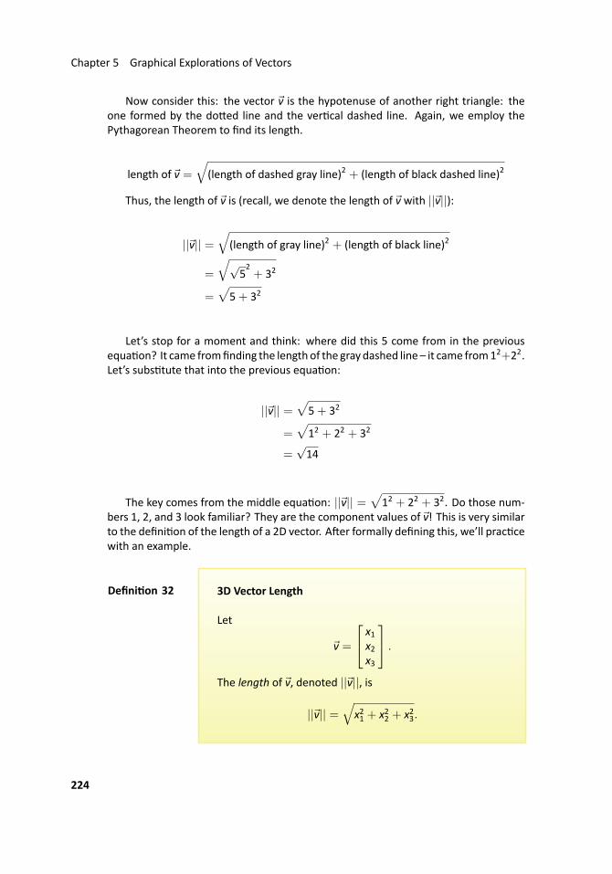
Chapter 5 Graphical Explora ons of Vectors
Now consider this: the vector v is the hypotenuse of another right triangle: theone formed by the do ed line and the ver cal dashed line. Again, we employ thePythagorean Theorem to find its length.
length of v =√
(length of dashed gray line)2 + (length of black dashed line)2
Thus, the length of v is (recall, we denote the length of v with ||v||):
||v|| =√
(length of gray line)2 + (length of black line)2
=
√√52+ 32
=√
5+ 32
Let’s stop for a moment and think: where did this 5 come from in the previousequa on? It came fromfinding the length of the gray dashed line – it came from12+22.Let’s subs tute that into the previous equa on:
||v|| =√
5+ 32
=√
12 + 22 + 32
=√14
The key comes from the middle equa on: ||v|| =√
12 + 22 + 32. Do those num-bers 1, 2, and 3 look familiar? They are the component values of v! This is very similarto the defini on of the length of a 2D vector. A er formally defining this, we’ll prac cewith an example.
..Defini on 32
.
.3D Vector Length
Let
v =
x1x2x3
.
The length of v, denoted ||v||, is
||v|| =√
x21 + x22 + x23.
224
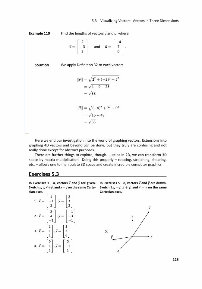
5.3 Visualizing Vectors: Vectors in Three Dimensions
.. Example 110 Find the lengths of vectors v and u, where
v =
2−35
and u =
−470
.
S We apply Defini on 32 to each vector:
||v|| =√
22 + (−3)2 + 52
=√4+ 9+ 25
=√38
||u|| =√
(−4)2 + 72 + 02
=√16+ 49
=√65
..
Here we end our inves ga on into the world of graphing vectors. Extensions intographing 4D vectors and beyond can be done, but they truly are confusing and notreally done except for abstract purposes.
There are further things to explore, though. Just as in 2D, we can transform 3Dspace by matrix mul plica on. Doing this properly – rota ng, stretching, shearing,etc. – allows one to manipulate 3D space and create incredible computer graphics.
Exercises 5.3In Exercises 1 – 4, vectors x and y are given.Sketch x, y, x+ y, and x− y on the same Carte-sian axes.
1. x =
1−12
, y = 232
2. x =
24−1
, y =−1−3−1
3. x =
112
, y = 336
4. x =
011
, y = 0−11
In Exercises 5 – 8, vectors x and y are drawn.Sketch 2x, −y, x + y, and x − y on the sameCartesian axes.
5...
x
. y.
z
.
x
.y
225
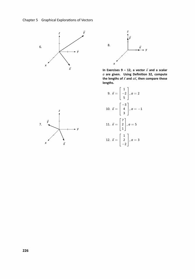
Chapter 5 Graphical Explora ons of Vectors
6...
x
. y.
z
.
x
.
y
7...
x
. y.
z
.
x
.
y
8...
x
. y.
z
. x.
y
In Exercises 9 – 12, a vector x and a scalara are given. Using Defini on 32, computethe lengths of x and ax, then compare theselengths.
9. x =
1−25
, a = 2
10. x =
−343
, a = −1
11. x =
721
, a = 5
12. x =
12−2
, a = 3
226
A .
S T S P
Chapter 1
Sec on 1.1
1. y
3. y
5. n
7. y
9. y
11. x = 1, y = −2
13. x = −1, y = 0, z = 2
15. 29 chickens and 33 pigs
Sec on 1.2
1.
3 4 5 7−1 1 −3 12 −2 3 5
3.
1 3 −4 5 17−1 0 4 8 12 3 4 5 6
5.
x1 + 2x2 = 3−x1 + 3x2 = 9
7.x1 + x2 − x3 − x4 = 2
2x1 + x2 + 3x3 + 5x4 = 7
9.x1 + x3 + 7x5 = 2
x2 + 3x3 + 2x4 = 5
11.
2 −1 75 0 30 4 −2
13.
2 −1 70 4 −25 8 −1
15.
2 −1 70 4 −20 5/2 −29/2
17. R1 + R2 → R2
19. R1 ↔ R2
21. x = 2, y = 1
23. x = −1, y = 0
25. x1 = −2, x2 = 1, x3 = 2
Sec on 1.3
1. (a) yes
(b) no
(c) no
(d) yes
3. (a) no
(b) yes
(c) yes
(d) yes
5.[1 00 1
]7.
[1 30 0
]9.
[1 0 30 1 7
]11.
[1 −1 20 0 0
]
13.
1 0 00 1 00 0 1
227
Chapter A Solu ons To Selected Problems
15.
1 0 00 1 00 0 1
17.
1 0 0 10 1 1 10 0 0 0
19.
1 0 1 30 1 −2 40 0 0 0
21.
[1 1 0 0 0 00 0 1 3 1 4
]Sec on 1.4
1. x1 = 1− 2x2; x2 is free. Possible solu ons:x1 = 1, x2 = 0 and x1 = −1, x2 = 1.
3. x1 = 1; x2 = 2
5. No solu on; the system is inconsistent.
7. x1 = −11+ 10x3; x2 = −4+ 4x3; x3 isfree. Possible solu ons: x1 = −11,x2 = −4, x3 = 0 and x1 = −1, x2 = 0 andx3 = 1.
9. x1 = 1− x2 − x4; x2 is free; x3 = 1− 2x4;x4 is free. Possible solu ons: x1 = 1,x2 = 0, x3 = 1, x4 = 0 and x1 = −2,x2 = 1, x3 = −3, x4 = 2
11. No solu on; the system is inconsistent.
13. x1 = 13 − 4
3 x3; x2 = 13 − 1
3 x3; x3 is free.Possible solu ons: x1 = 1
3 , x2 = 13 , x3 = 0
and x1 = −1, x2 = 0, x3 = 1
15. Never exactly 1 solu on; infinite solu ons ifk = 2; no solu on if k = 2.
17. Exactly 1 solu on if k = 2; no solu on ifk = 2; never infinite solu ons.
Sec on 1.5
1. 29 chickens and 33 pigs
3. 42 grande tables, 22 ven tables
5. 30 men, 15 women, 20 kids
7. f(x) = −2x+ 10
9. f(x) = 12 x
2 + 3x+ 1
11. f(x) = 3
13. f(x) = x3 + 1
15. f(x) = 32 x+ 1
17. The augmented matrix from this system is 1 1 1 1 86 1 2 3 240 1 −1 0 0
. From this we
find the solu on
t =8
3−
1
3f
x =8
3−
1
3f
w =8
3−
1
3f.
The only me each of these variables arenonnega ve integers is when f = 2 orf = 8. If f = 2, then we have 2touchdowns, 2 extra points and 2 two pointconversions (and 2 field goals); this doesn’tmake sense since the extra points and twopoint conversions follow touchdowns. Iff = 8, then we have no touchdowns, extrapoints or two point conversions (just 8 fieldgoals). This is the only solu on; all pointswere scored from field goals.
19. Let x1, x2 and x3 represent the number offree throws, 2 point and 3 point shotstaken. The augmented matrix from this
system is[1 1 1 301 2 3 80
]. From this we
find the solu on
x1 = −20+ x3x2 = 50− 2x3.
In order for x1 and x2 to be nonnega ve, weneed 20 ≤ x3 ≤ 25. Thus there are 6different scenerios: the “first” is where 20three point shots are taken, no free throws,and 10 two point shots; the “last” is where25 three point shots are taken, 5 freethrows, and no two point shots.
21. Let y = ax+ b; all linear func ons through(1,3) come in the form y = (3− b)x+ b.Examples: b = 0 yields y = 3x; b = 2yields y = x+ 2.
23. Let y = ax2 + bx+ c; we find thata = − 1
2 + 12 c and b = 1
2 − 32 c. Examples:
c = 1 yields y = −x+ 1; c = 3 yieldsy = x2 − 4x+ 3.
Chapter 2
Sec on 2.1
1.[−2 −112 13
]3.
[2 −214 8
]
228
5.[
9 −711 −6
]7.
[−146
]9.
[−15−25
]11. X =
[−5 9−1 −14
]13. X =
[−5 −2
−9/2 −19/2
]15. a = 2, b = 1
17. a = 5/2+ 3/2b
19. No solu on.
21. No solu on.
Sec on 2.2
1. −22
3. 0
5. 5
7. 15
9. −2
11. Not possible.
13. AB =
[8 310 −9
]BA =
[−3 244 2
]15. AB =
[−1 −2 1210 4 32
]BA is not possible.
17. AB is not possible.
BA =
[27 −33 39−27 −3 −15
]
19. AB =
−32 34 −24−32 38 −8−16 21 4
BA =
[22 −14−4 −12
]
21. AB =
−56 2 −3620 19 −30−50 −13 0
BA =
[−46 4072 9
]23. AB =
[−15 −22 −21 −116 −53 −59 −31
]BA is not possible.
25. AB =
0 0 46 4 −22 −4 −6
BA =
2 −2 62 2 44 0 −6
27. AB =
21 −17 −519 5 195 9 4
BA =
19 5 235 −7 −1
−14 6 18
29. DA =
[4 −64 −6
]AD =
[4 8−3 −6
]
31. DA =
2 2 2−6 −6 −6−15 −15 −15
AD =
2 −3 54 −6 10−6 9 −15
33. DA =
d1a d1b d1cd2d d2e d2fd3g d3h d3i
AD =
d1a d2b d3cd1d d2e d3fd1g d2h d3i
35. Ax =
[−611
]
37. Ax =
−5521
39. Ax =
x1 + 2x2 + 3x3x1 + 2x3
2x1 + 3x2 + x3
41. A2 =
[4 00 9
]; A3 =
[8 00 27
]
43. A2 =
0 0 11 0 00 1 0
; A3 =
1 0 00 1 00 0 1
45. (a)
[0 −2−5 −1
](b)
[10 25 11
](c)
[−11 −1537 32
](d) No.
(e) (A+B)(A+B) = AA+AB+BA+BB =A2 + AB+ BA+ B2.
229
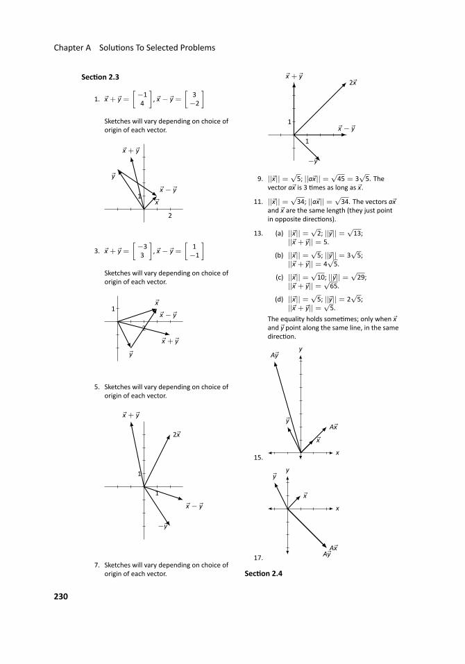
Chapter A Solu ons To Selected Problems
Sec on 2.3
1. x + y =[−14
], x − y =
[3−2
]Sketches will vary depending on choice oforigin of each vector.
..2
.
1
.x
.
y
.
x + y
.
x − y
3. x + y =[−33
], x − y =
[1−1
]Sketches will vary depending on choice oforigin of each vector.
..2
.
1
.
x
.
y
.
x + y
.x − y
5. Sketches will vary depending on choice oforigin of each vector.
..1
.
1
.
2x
.
−y
.
x + y
.
x − y
7. Sketches will vary depending on choice oforigin of each vector.
..1
.
1
.
2x
.
−y
.
x + y
. x − y
9. ||x|| =√5; ||ax|| =
√45 = 3
√5. The
vector ax is 3 mes as long as x.
11. ||x|| =√34; ||ax|| =
√34. The vectors ax
and x are the same length (they just pointin opposite direc ons).
13. (a) ||x|| =√2; ||y|| =
√13;
||x + y|| = 5.
(b) ||x|| =√5; ||y|| = 3
√5;
||x + y|| = 4√5.
(c) ||x|| =√10; ||y|| =
√29;
||x + y|| =√65.
(d) ||x|| =√5; ||y|| = 2
√5;
||x + y|| =√5.
The equality holds some mes; only when xand y point along the same line, in the samedirec on.
15... x.
y
.
x
.
y
.
Ax
.
Ay
17.
.. x.
y
.
x
.
y
.
Ax
.
Ay
Sec on 2.4
230
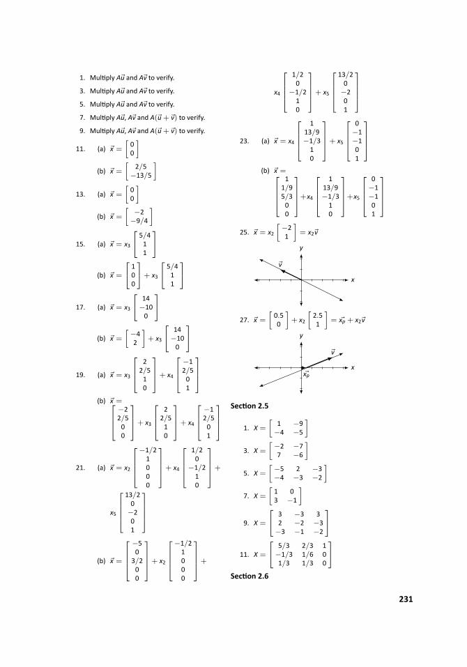
1. Mul ply Au and Av to verify.
3. Mul ply Au and Av to verify.
5. Mul ply Au and Av to verify.
7. Mul ply Au, Av and A(u+ v) to verify.
9. Mul ply Au, Av and A(u+ v) to verify.
11. (a) x =
[00
](b) x =
[2/5
−13/5
]13. (a) x =
[00
](b) x =
[−2
−9/4
]
15. (a) x = x3
5/411
(b) x =
100
+ x3
5/411
17. (a) x = x3
14−100
(b) x =
[−42
]+ x3
14−100
19. (a) x = x3
2
2/510
+ x4
−12/501
(b) x =
−22/500
+ x3
2
2/510
+ x4
−12/501
21. (a) x = x2
−1/21000
+ x4
1/20
−1/210
+
x5
13/20−201
(b) x =
−50
3/200
+ x2
−1/21000
+
x4
1/20
−1/210
+ x5
13/20−201
23. (a) x = x4
1
13/9−1/310
+ x5
0−1−101
(b) x =
11/95/300
+x4
1
13/9−1/310
+x5
0−1−101
25. x = x2
[−21
]= x2v
.. x.
y
.
v
27. x =
[0.50
]+ x2
[2.51
]= xp + x2v
.. x.
y
.xp.
v
Sec on 2.5
1. X =
[1 −9−4 −5
]3. X =
[−2 −77 −6
]5. X =
[−5 2 −3−4 −3 −2
]7. X =
[1 03 −1
]
9. X =
3 −3 32 −2 −3−3 −1 −2
11. X =
5/3 2/3 1−1/3 1/6 01/3 1/3 0
Sec on 2.6
231
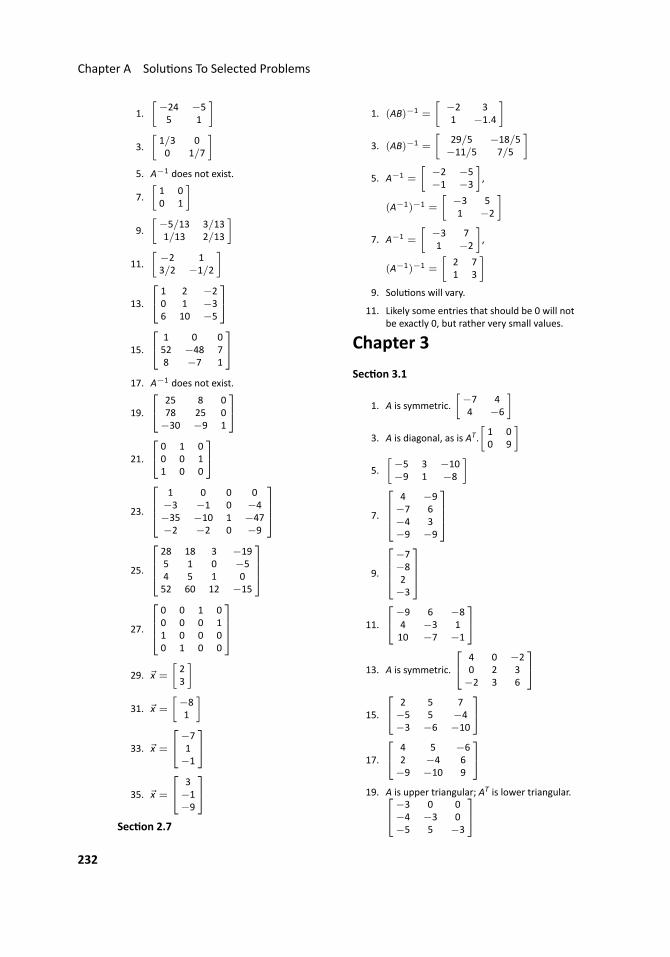
Chapter A Solu ons To Selected Problems
1.[−24 −55 1
]3.
[1/3 00 1/7
]5. A−1 does not exist.
7.[1 00 1
]9.
[−5/13 3/131/13 2/13
]11.
[−2 13/2 −1/2
]
13.
1 2 −20 1 −36 10 −5
15.
1 0 052 −48 78 −7 1
17. A−1 does not exist.
19.
25 8 078 25 0−30 −9 1
21.
0 1 00 0 11 0 0
23.
1 0 0 0−3 −1 0 −4−35 −10 1 −47−2 −2 0 −9
25.
28 18 3 −195 1 0 −54 5 1 052 60 12 −15
27.
0 0 1 00 0 0 11 0 0 00 1 0 0
29. x =
[23
]31. x =
[−81
]
33. x =
−71−1
35. x =
3−1−9
Sec on 2.7
1. (AB)−1 =
[−2 31 −1.4
]3. (AB)−1 =
[29/5 −18/5−11/5 7/5
]5. A−1 =
[−2 −5−1 −3
],
(A−1)−1 =
[−3 51 −2
]7. A−1 =
[−3 71 −2
],
(A−1)−1 =
[2 71 3
]9. Solu ons will vary.
11. Likely some entries that should be 0 will notbe exactly 0, but rather very small values.
Chapter 3
Sec on 3.1
1. A is symmetric.[−7 44 −6
]3. A is diagonal, as is AT.
[1 00 9
]5.
[−5 3 −10−9 1 −8
]
7.
4 −9−7 6−4 3−9 −9
9.
−7−82−3
11.
−9 6 −84 −3 110 −7 −1
13. A is symmetric.
4 0 −20 2 3−2 3 6
15.
2 5 7−5 5 −4−3 −6 −10
17.
4 5 −62 −4 6−9 −10 9
19. A is upper triangular; AT is lower triangular. −3 0 0
−4 −3 0−5 5 −3
232
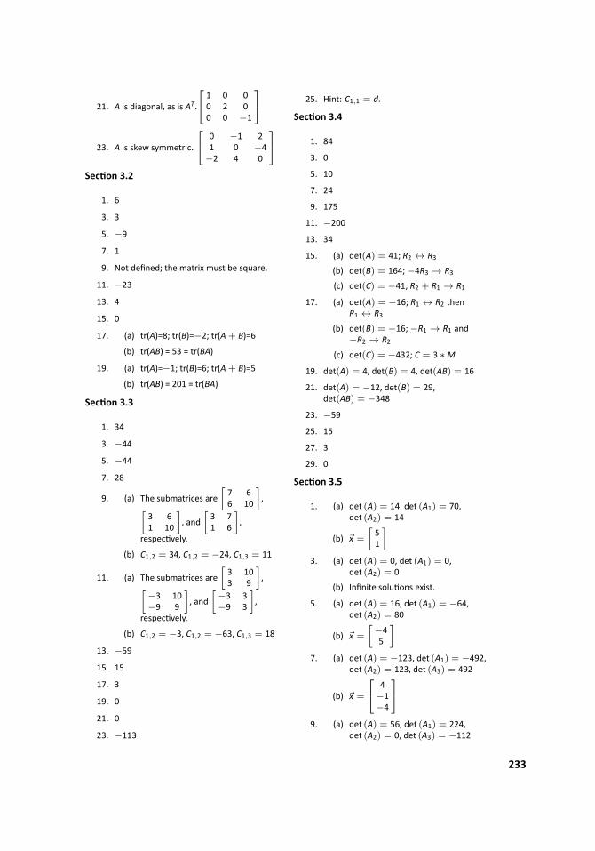
21. A is diagonal, as is AT.
1 0 00 2 00 0 −1
23. A is skew symmetric.
0 −1 21 0 −4−2 4 0
Sec on 3.2
1. 6
3. 3
5. −9
7. 1
9. Not defined; the matrix must be square.
11. −23
13. 4
15. 0
17. (a) tr(A)=8; tr(B)=−2; tr(A+ B)=6
(b) tr(AB) = 53 = tr(BA)
19. (a) tr(A)=−1; tr(B)=6; tr(A+ B)=5
(b) tr(AB) = 201 = tr(BA)
Sec on 3.3
1. 34
3. −44
5. −44
7. 28
9. (a) The submatrices are[7 66 10
],[
3 61 10
], and
[3 71 6
],
respec vely.
(b) C1,2 = 34, C1,2 = −24, C1,3 = 11
11. (a) The submatrices are[3 103 9
],[
−3 10−9 9
], and
[−3 3−9 3
],
respec vely.
(b) C1,2 = −3, C1,2 = −63, C1,3 = 18
13. −59
15. 15
17. 3
19. 0
21. 0
23. −113
25. Hint: C1,1 = d.
Sec on 3.4
1. 84
3. 0
5. 10
7. 24
9. 175
11. −200
13. 34
15. (a) det(A) = 41; R2 ↔ R3
(b) det(B) = 164;−4R3 → R3
(c) det(C) = −41; R2 + R1 → R1
17. (a) det(A) = −16; R1 ↔ R2 thenR1 ↔ R3
(b) det(B) = −16;−R1 → R1 and−R2 → R2
(c) det(C) = −432; C = 3 ∗M
19. det(A) = 4, det(B) = 4, det(AB) = 16
21. det(A) = −12, det(B) = 29,det(AB) = −348
23. −59
25. 15
27. 3
29. 0
Sec on 3.5
1. (a) det (A) = 14, det (A1) = 70,det (A2) = 14
(b) x =
[51
]3. (a) det (A) = 0, det (A1) = 0,
det (A2) = 0
(b) Infinite solu ons exist.
5. (a) det (A) = 16, det (A1) = −64,det (A2) = 80
(b) x =
[−45
]7. (a) det (A) = −123, det (A1) = −492,
det (A2) = 123, det (A3) = 492
(b) x =
4−1−4
9. (a) det (A) = 56, det (A1) = 224,
det (A2) = 0, det (A3) = −112
233
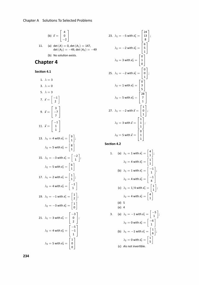
Chapter A Solu ons To Selected Problems
(b) x =
40−2
11. (a) det (A) = 0, det (A1) = 147,
det (A2) = −49, det (A3) = −49
(b) No solu on exists.
Chapter 4
Sec on 4.1
1. λ = 3
3. λ = 0
5. λ = 3
7. x =
[−12
]
9. x =
3−77
11. x =
−111
13. λ1 = 4 with x1 =
[91
];
λ2 = 5 with x2 =
[81
]
15. λ1 = −3 with x1 =
[−21
];
λ2 = 5 with x2 =
[61
]
17. λ1 = 2 with x1 =
[11
];
λ2 = 4 with x2 =
[−11
]
19. λ1 = −1 with x1 =
[12
];
λ2 = −3 with x2 =
[10
]
21. λ1 = 3 with x1 =
−302
;λ2 = 4 with x2 =
−5−11
λ3 = 5 with x3 =
100
23. λ1 = −5 with x1 =
24138
;λ2 = −2 with x2 =
651
λ3 = 3 with x3 =
010
25. λ1 = −2 with x1 =
001
;λ2 = 1 with x2 =
035
λ3 = 5 with x3 =
2871
27. λ1 = −2 with x =
101
;λ2 = 3 with x =
111
;λ3 = 5 with x =
011
Sec on 4.2
1. (a) λ1 = 1 with x1 =
[41
];
λ2 = 4 with x2 =
[11
](b) λ1 = 1 with x1 =
[−11
];
λ2 = 4 with x2 =
[−14
](c) λ1 = 1/4 with x1 =
[11
];
λ2 = 4 with x2 =
[41
](d) 5
(e) 4
3. (a) λ1 = −1 with x1 =
[−51
];
λ2 = 0 with x2 =
[−61
](b) λ1 = −1 with x1 =
[16
];
λ2 = 0 with x2 =
[15
](c) Ais not inver ble.
234
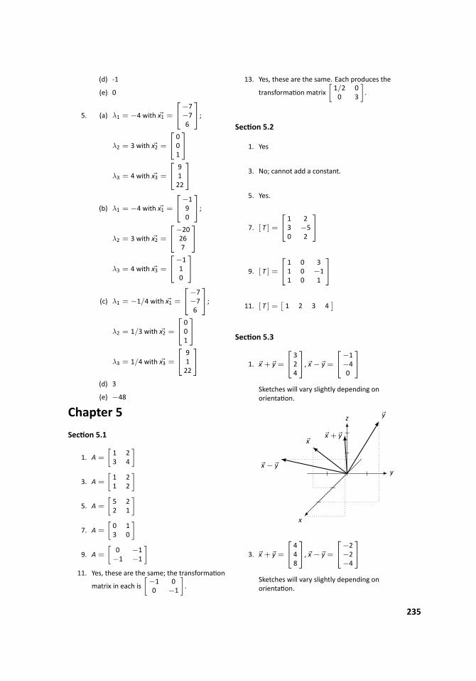
(d) -1
(e) 0
5. (a) λ1 = −4 with x1 =
−7−76
;λ2 = 3 with x2 =
001
λ3 = 4 with x3 =
9122
(b) λ1 = −4 with x1 =
−190
;λ2 = 3 with x2 =
−20267
λ3 = 4 with x3 =
−110
(c) λ1 = −1/4 with x1 =
−7−76
;λ2 = 1/3 with x2 =
001
λ3 = 1/4 with x3 =
9122
(d) 3
(e) −48
Chapter 5
Sec on 5.1
1. A =
[1 23 4
]3. A =
[1 21 2
]5. A =
[5 22 1
]7. A =
[0 13 0
]9. A =
[0 −1−1 −1
]11. Yes, these are the same; the transforma on
matrix in each is[−1 00 −1
].
13. Yes, these are the same. Each produces the
transforma on matrix[1/2 00 3
].
Sec on 5.2
1. Yes
3. No; cannot add a constant.
5. Yes.
7. [ T ] =
1 23 −50 2
9. [ T ] =
1 0 31 0 −11 0 1
11. [ T ] =[1 2 3 4
]
Sec on 5.3
1. x + y =
324
, x − y =
−1−40
Sketches will vary slightly depending onorienta on.
..
x
. y.
z
.
y
.
x
.
x + y
.x − y
3. x + y =
448
, x − y =
−2−2−4
Sketches will vary slightly depending onorienta on.
235
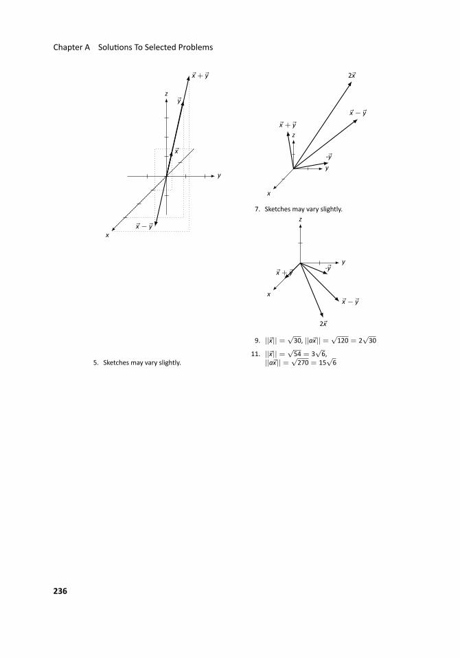
Chapter A Solu ons To Selected Problems
..
x
. y.
z
.
x
.
y
.
x + y
.
x − y
5. Sketches may vary slightly.
..
x
. y.
z
.
2x
.-y
.
x + y
.
x − y
7. Sketches may vary slightly.
..
x
. y.
z
.
2x
.-y
.
x + y
.
x − y
9. ||x|| =√30, ||ax|| =
√120 = 2
√30
11. ||x|| =√54 = 3
√6,
||ax|| =√270 = 15
√6
236

Index
an symmetric, 128augmented matrix, 8
basic variable, 27
characteris c polynomial, 168cofactor, 137
expansion, 139, 146consistent, 24, 88, 90Cramer’s Rule, 159
determinant3× 3 shortcut, 155and elementary row opera ons, 150defini on, 141of 2× 2 matrices, 136of triangular matrices, 148proper es, 154
diagonal, 118defini on, 123
eigenvaluedefini on, 164finding, 168proper es, 182
eigenvector, see eigenvalueelementary row opera ons, 13
and determinants, 150
free variable, 25, 27
Gaussian elimina on, 15, 18backward steps, 17forward steps, 17
homogeneous, 87, 88, 90
iden ty matrix, 61
inconsistent, 24inverse
compu ng, 107defini on, 106Inver ble Matrix Theorem, 113proper es, 113, 119uniqueness, 106
Inver ble Matrix Theorem, 113, 155, 183
leading one, 14, 27, 29linear equa on, 3linear transforma on
and 0, 208condi ons on, 213defini on, 204standard matrix of, 207, 209
matrixaddi on, 47arithme c proper es, 49augmented, 8cofactor, 137defini on, 7determinant, 136, 141diagonal, 123equality, 46iden ty matrix, 61inverse, 106, 107minor, 137mul plica on, 54
proper es, 62scalar mul plica on, 47the zero matrix, 49transpose, 122triangular, 123
minor, 137
Parallelogram Law, 69
237

Index
par cular solu on, 30problem solving, 37pseudoinverse, 130
reduced echelon form, 14reduced row echelon form, 14row echelon form, 14
skew symmetric, 128defini on, 128theorem, 129
solu on, 3infinite, 24, 27, 90none, 24par cular, 30types, 24unique, 24, 90, 110
standard unit vector, 208symmetric, 128
defini on, 128theorem, 129
system of linear equa onsconsistent, 24, 27, 88, 90defini on, 3homogeneous, 87inconsistent, 24, 29solu on, 3
tracedefini on, 131proper es, 133
transpose, 121defini on, 122proper es, 126skew-symmetric, 128symmetric, 128
triangular matrixdefini on, 123determinant, 148
variablebasic, 27dependent, 27free, 25, 27independent, 27
vector
column, 52length, 74, 224row, 52
zero matrix, 49
238