Functions of Bounded Higher Variation - ETH Zhmsoner/pdfs/46-Soner-bnv-02.pdf · Functions of...

Functions of Bounded Higher VariationR.L. JERRARD & H.M. SONER

ABSTRACT. We say that a function u : Rm ! Rn, withm " n,has bounded n-variation if Det(ux!1

, . . . , ux!n ) is a measure forevery 1 # !1 < · · · < !n # m. Here Det(v1, . . . , vn) denotesthe distributional determinant of the matrix whose columns arethe given vectors, arranged in the given order.

In this paper we establish a number of properties of BnV func-tions and related functions. We establish general (and ratherweak) versions of the chain rule and the coarea formula; we showthat stronger forms of the chain rule can fail, and we also demon-strate that BnV functions cannot, in general, be strongly approxi-mated by smooth functions; and we prove that if u $BnV(Rm,Rn) and |u| = 1 a.e., then the Jacobian of u is anm%n-dimensional rectifiable current.

1. INTRODUCTION

Given a function u : Rm & U ! Rn with n # m, we define the distributionalJacobian [Ju] of u to be the pullback by u (in the sense of distributions) of thestandard volume form on Rn, so that

(1.1) [Ju] =!

!$In,mDet(ux!1

, . . . , ux!n )dx!.

Here In,m is the set of all multiindices of the form ! = (!1, . . . ,!n) such that 1 #!1 < · · · < !n #m. For such a multiindex, dx! := dx!1 ' · · · ' dx!n . Detdenotes the distributional determinant, the definition of which is given in Section2. The definition of [Ju] makes sense if for example u $ W 1,n%1

loc ( L)loc(U ;Rn).We say that a function has locally bounded n-variation in U if for every

bounded open set V ** U there exists some constant C = C(V) such that

(1.2)!

!$In,m

""! Det(ux!1

, . . . , ux!n ) := +", [Ju], # C-"-C0

645

646 R.L. JERRARD & H.M. SONER

for all C1 n-forms " =#!$In,n"! dx! with support in V . When this holds we

write u $ BnVloc(U ;Rn).If C can be chosen independently of V , then we say that u has bounded n-

variation in U , and we write u $ BnV(U ;Rn).If u $ BnVloc(U ;Rn), the Riesz Representation Theorem asserts that there

is a nonnegative Radon measure, which we denote |Ju|, and a |Ju|-measurablefunction # : U ! $nRm such that

|#(x)| = 1 |Ju| almost every x; and

+", [Ju], =""(x) · #(x)d|Ju|.

Moreover, |Ju| satisfies

(1.3) |Ju|(V) = sup{+", [Ju], |" $ C1c (V ;$nRm); |"| # 1 in V}

for every open V * U .When u $ BnVloc we also write

%$ · [Ju] for +$, [Ju],.

We will chiefly be interested in the case where [Ju] cannot be represented byan L1 function.

Results. The definition of BnV more or less generalizes that of the classicalspace BV , and many results about BV have some sort of generalization in BnV .The first result we state is an analogue of the theorem of De Giorgi on the rectifi-ability of the reduced boundary of a set of finite perimeter.

We write u $ BnVloc(U ;Sn%1) to mean that u $ BnVloc(U ;Rn) with |u| =1 almost everywhere. We write "n to denote the volume of the unit ball in Rn.

Theorem 1.1. If u $ W 1,n%1(BnVloc(U ;Sn%1), then there exists an (m%n)-dimensional rectifiable set & and a positive integer-valuedHm%n-measurable function% : & ! Z, such that

(1.4)"$ · [Ju] ="n

"

&%$ · # dHm%n

for all $ $ C0c (Rm;$nRm). In addition, #(x) represents an oriented unit n-vector

normal to & at Hm%n a.e. x $ & .This theorem is an easy consequence of known results, but as far as we know

it was not explicitly pointed out before our work. We will give two proofs, one ofwhich is due to M. Giaquinta and G. Modica. After learning of our result, Linand Hang [20] gave a quick proof of a result very similar to Theorem 1.1, forfunctions u $ W 1%1/n,n(Rm;Sn%1) such that the distributional pullback of thevolume form on Rn is a measure.

Rectifiable sets and related geometric background are discussed in many ref-erences; see for example [17], Section 2.1.4.

Functions of Bounded Higher Variation 647

In the statement of our next result we use the notation

ua(x) =u(x)% a|u(x)% a| for u : Rm ! Rn, a $ Rn.

If u is a smooth function and a is a regular value of u, then simple examples leadone to expect that [Jua] should be a unit multiplicity measure whose supportis exactly the level set {x | u(x) = a}. More generally we think of [Jua] as aweak, measure-theoretic representation of the level set {u(x) = a}; note in thiscontext that in view of Theorem 1.1, if ua $ BnV then [Jua] is carried by a(m%n)-dimensional rectifiable set.

These considerations lead us to interpret (1.5) as a weak form of the coareaformula.

Theorem 1.2. If u $ W 1,n%1loc (L)loc(Rm;Rn), then ua $ W 1,n%1

loc (L) for a.e.a $ Rn, and

(1.5) [Ju] = 1"n

"

a$Rn[Jua]da

in the sense of distributions.If u $ W 1,p

loc ( L)loc(Rm;Rn) for some p > n % 1, and if F $ W 1,)(Rn;Rn)and w = F(u), then

(1.6) +", [Jw], = 1"n

"

a$RnJF(a)+", [Jua],da

for all " $ C1c (Rm;$nRm). This remains true if u $ W 1,n%1

loc ( C0, or if u $W 1,n%1 ( L)loc and F $ C1.

If, in addition, u $ BnV(Rm;Rn) and either u $ W 1,p for some p > n, or|u| = 1 a.e., then ua $ BnV(Rm;Sn%1) for a.e. a $ Rn, and

(1.7) |Ju|(A) = 1"n

"

a$Rn|Jua|(A)da

for every Borel set A * Rm.

We refer to (1.5) as the weak coarea formula, and to (1.7) as the strong coareaformula.

Remark 1.3. Observe that (1.5) and (1.6) do not require u $ BnVloc.

Our next result details some ways in which BnV fails to inherit certain niceproperties of BV .


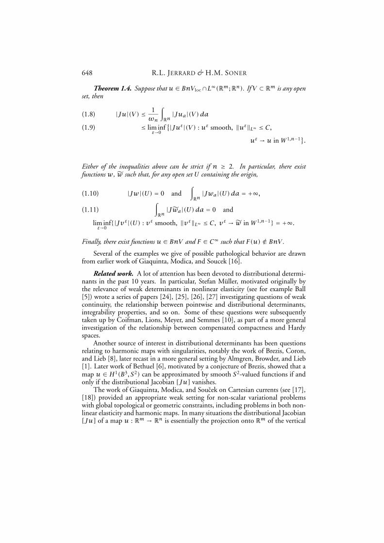
Theorem 1.4. Suppose that u $ BnVloc(L)(Rm;Rn). If V * Rm is any openset, then

|Ju|(V) # 1"n

"

Rn|Jua|(V)da(1.8)

# lim inf&!0

'|Ju&|(V) : u& smooth, -u&-L) # C,(1.9)

u& ! u in W 1,n%1(.

Either of the inequalities above can be strict if n " 2. In particular, there existfunctions w, )w such that, for any open set U containing the origin,

|Jw|(U) = 0 and"

Rn|Jwa|(U)da = +),(1.10)

"

Rn|J)wa|(U)da = 0 and(1.11)

lim inf&!0

{|Jv&|(U) : v& smooth, -v&-L) # C, v& ! )w in W 1,n%1} = +).

Finally, there exist functions u $ BnV and F $ C) such that F(u) .$ BnV .

Several of the examples we give of possible pathological behavior are drawnfrom earlier work of Giaquinta, Modica, and Soucek [16].

Related work. A lot of attention has been devoted to distributional determi-nants in the past 10 years. In particular, Stefan Muller, motivated originally bythe relevance of weak determinants in nonlinear elasticity (see for example Ball[5]) wrote a series of papers [24], [25], [26], [27] investigating questions of weakcontinuity, the relationship between pointwise and distributional determinants,integrability properties, and so on. Some of these questions were subsequentlytaken up by Coifman, Lions, Meyer, and Semmes [10], as part of a more generalinvestigation of the relationship between compensated compactness and Hardyspaces.

Another source of interest in distributional determinants has been questionsrelating to harmonic maps with singularities, notably the work of Brezis, Coron,and Lieb [8], later recast in a more general setting by Almgren, Browder, and Lieb[1]. Later work of Bethuel [6], motivated by a conjecture of Brezis, showed that amap u $ H1(B3, S2) can be approximated by smooth S2-valued functions if andonly if the distributional Jacobian [Ju] vanishes.

The work of Giaquinta, Modica, and Soucek on Cartesian currents (see [17],[18]) provided an appropriate weak setting for non-scalar variational problemswith global topological or geometric constraints, including problems in both non-linear elasticity and harmonic maps. In many situations the distributional Jacobian[Ju] of a map u : Rm ! Rn is essentially the projection onto Rm of the vertical


part of a Cartesian current that, roughly speaking, corresponds to the graph ofu with holes “filled in”. Thus our work is very closely related to Cartesian cur-rents. Indeed, some of our ideas are implicit in the work of Giaquinta, Modica,and Soucek, and some of our results become very transparent when viewed in theframework of Cartesian currents. These connections are discussed in more detailin Section 6.

Organization. Section 2 gives the definition and basic properties of distri-butional Jacobians, and also summarizes some notation. Section 3 contains anumber of examples, some of which are part of the proof of Theorem 1.4. Section4 is mainly devoted to the proof of Theorem 1.2, though it also cleans up someloose ends in Theorem 1.4. The proofs of these two theorems are summarized atthe beginning of Section 4.

In Sections 5 and 6 we give two proofs of Theorem 1.1. The first uses slicingproperties of [Ju], and the second, due to M. Giaquinta and L. Modica, usessome ideas about Cartesian currents.

Acknowledgments. We gratefully acknowledge useful and interesting discus-sions with Giovanni Alberti, Luigi Ambrosio, and Haım Brezis. The rectifiabilityproof in Section 6 was communicated to us by M. Giaquinta and L. Modica,and we are very grateful to them for pointing it out. We are also grateful to ananonymous referee for some useful suggestions.

R.L. Jerrard was partially supported by NSF grant DMS 99-70273.H.M. Soner was partially supported by the Army Research O!ce and the Na-tional Science Foundation through the Center for Nonlinear Analysis at CarnegieMellon University, and by NSF grant 98-17525 and ARO grant DAAH04-95-1-0226. Parts of this paper were completed during visits of Jerrard to the Centerfor Nonlinear Analysis, and other parts while Soner was visiting the Feza GurseyInstitute for Basic Sciences in Istanbul.

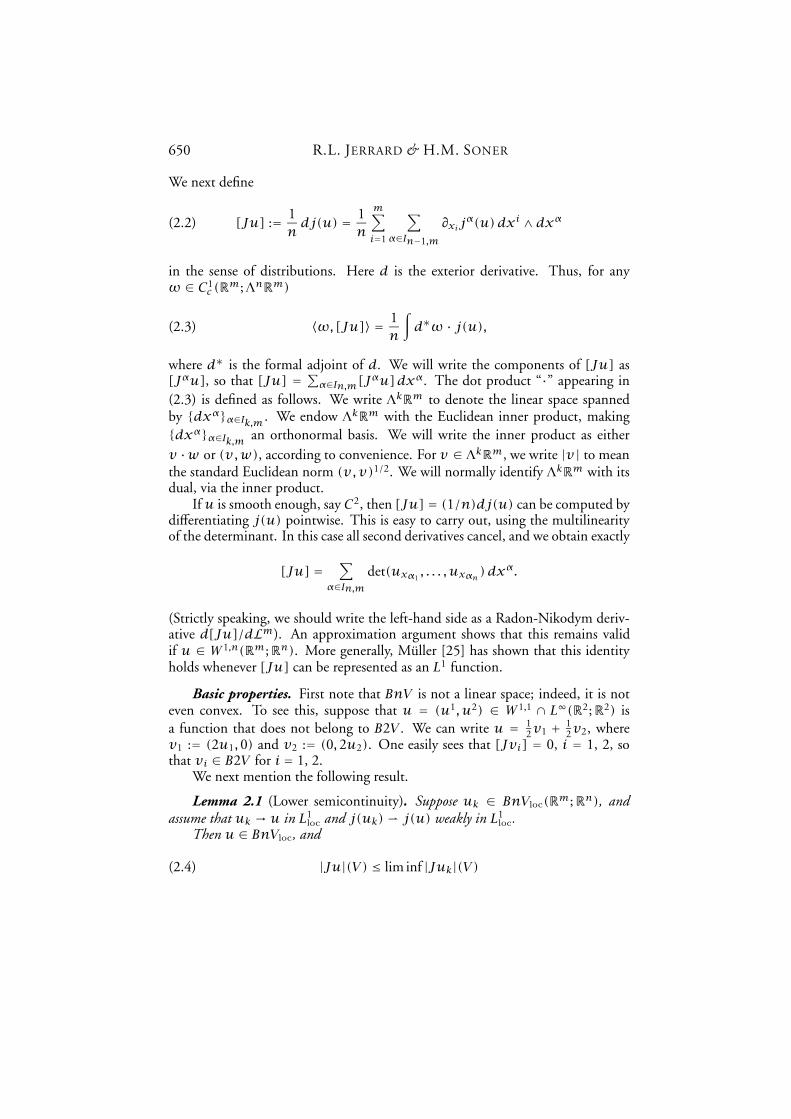
2. DEFINITIONS AND BASIC PROPERTIES

Definitions. For su!ciently smooth functions u : Rm ! Rn, we define ann% 1 form

(2.1) j(u) :=!

!$In%1,m

det(u,ux!1, . . . , ux!n%1

)dx!.

For our purposes, “su!ciently smooth” will mean that u belongs to a Sobolevspace in which j(u) is necessarily locally integrable, for exampleu $ W 1,n%1

loc (L)loc

or u $ W 1,ploc , p "mn/(m+ 1). One could relax this requirement somewhat; we

will not pursue this here.We will write the components of j(u) as j!(u), so that

j(u) =!

In%1,m

j!(u)dx!.


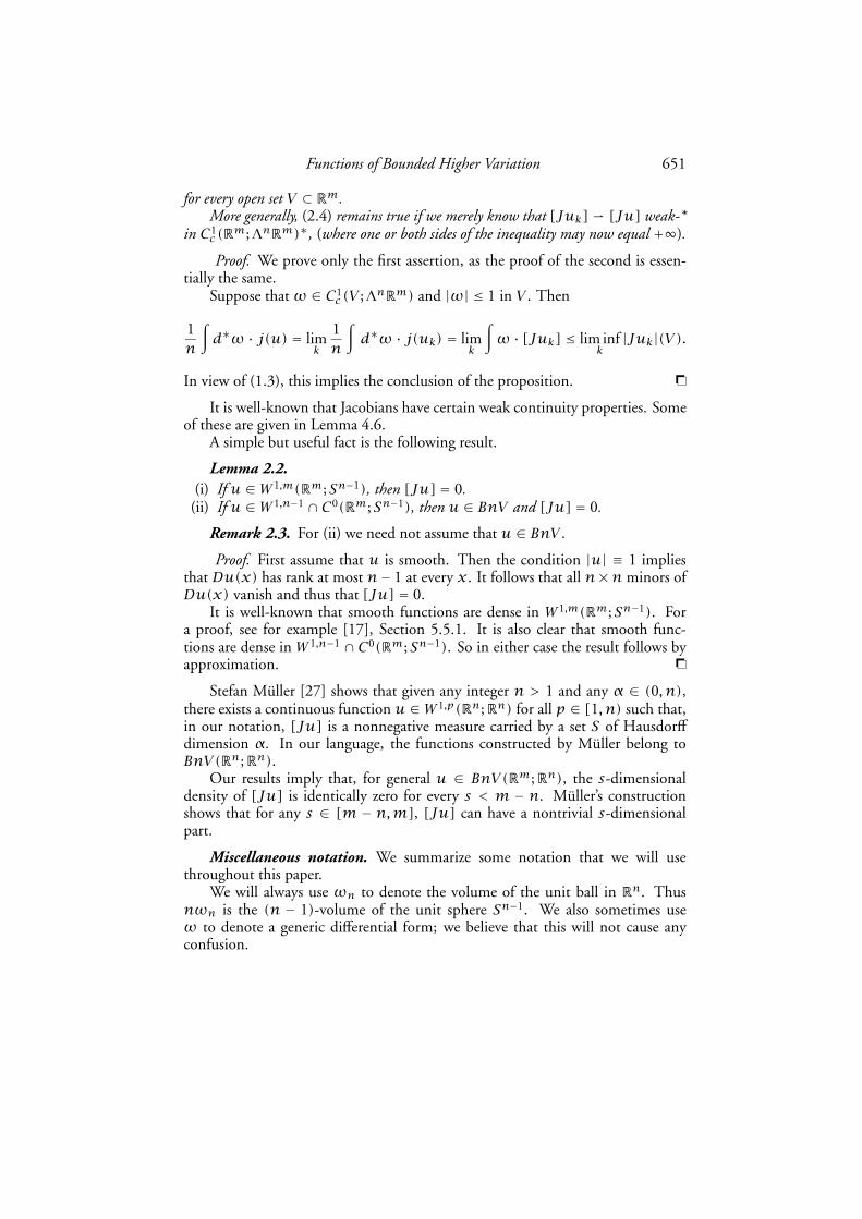
We next define

(2.2) [Ju] := 1ndj(u) = 1

n

m!

i=1

!

!$In%1,m

'xij!(u)dxi ' dx!

in the sense of distributions. Here d is the exterior derivative. Thus, for any" $ C1

c (Rm;$nRm)

(2.3) +", [Ju], = 1n

"d/" · j(u),

where d/ is the formal adjoint of d. We will write the components of [Ju] as[J!u], so that [Ju] =

#!$In,m[J!u]dx!. The dot product “·” appearing in

(2.3) is defined as follows. We write $kRm to denote the linear space spannedby {dx!}!$Ik,m . We endow $kRm with the Euclidean inner product, making{dx!}!$Ik,m an orthonormal basis. We will write the inner product as eitherv ·w or (v,w), according to convenience. For v $ $kRm, we write |v| to meanthe standard Euclidean norm (v, v)1/2. We will normally identify $kRm with itsdual, via the inner product.

If u is smooth enough, say C2, then [Ju] = (1/n)dj(u) can be computed bydi"erentiating j(u) pointwise. This is easy to carry out, using the multilinearityof the determinant. In this case all second derivatives cancel, and we obtain exactly

[Ju] =!

!$In,mdet(ux!1

, . . . , ux!n )dx!.

(Strictly speaking, we should write the left-hand side as a Radon-Nikodym deriv-ative d[Ju]/dLm). An approximation argument shows that this remains validif u $ W 1,n(Rm;Rn). More generally, Muller [25] has shown that this identityholds whenever [Ju] can be represented as an L1 function.

Basic properties. First note that BnV is not a linear space; indeed, it is noteven convex. To see this, suppose that u = (u1, u2) $ W 1,1 ( L)(R2;R2) isa function that does not belong to B2V . We can write u = 1

2v1 + 12v2, where

v1 := (2u1,0) and v2 := (0,2u2). One easily sees that [Jvi] = 0, i = 1, 2, sothat vi $ B2V for i = 1, 2.

We next mention the following result.

Lemma 2.1 (Lower semicontinuity). Suppose uk $ BnVloc(Rm;Rn), andassume that uk ! u in L1

loc and j(uk)( j(u) weakly in L1loc.

Then u $ BnVloc, and

(2.4) |Ju|(V) # lim inf |Juk|(V)


for every open set V * Rm.More generally, (2.4) remains true if we merely know that [Juk]( [Ju] weak-*

in C1c (Rm;$nRm)/, (where one or both sides of the inequality may now equal +)).

Proof. We prove only the first assertion, as the proof of the second is essen-tially the same.

Suppose that " $ C1c (V ;$nRm) and |"| # 1 in V . Then

1n

"d/" · j(u) = lim

k

1n

"d/" · j(uk) = lim

k

"" · [Juk] # lim inf

k|Juk|(V).

In view of (1.3), this implies the conclusion of the proposition. !

It is well-known that Jacobians have certain weak continuity properties. Someof these are given in Lemma 4.6.

A simple but useful fact is the following result.

Lemma 2.2.(i) If u $ W 1,m(Rm;Sn%1), then [Ju] = 0.

(ii) If u $ W 1,n%1 ( C0(Rm;Sn%1), then u $ BnV and [Ju] = 0.

Remark 2.3. For (ii) we need not assume that u $ BnV .

Proof. First assume that u is smooth. Then the condition |u| 0 1 impliesthat Du(x) has rank at most n% 1 at every x. It follows that all n1n minors ofDu(x) vanish and thus that [Ju] = 0.

It is well-known that smooth functions are dense in W 1,m(Rm;Sn%1). Fora proof, see for example [17], Section 5.5.1. It is also clear that smooth func-tions are dense in W 1,n%1 ( C0(Rm;Sn%1). So in either case the result follows byapproximation. !

Stefan Muller [27] shows that given any integer n > 1 and any ! $ (0, n),there exists a continuous function u $ W 1,p(Rn;Rn) for all p $ [1, n) such that,in our notation, [Ju] is a nonnegative measure carried by a set S of Hausdor"dimension !. In our language, the functions constructed by Muller belong toBnV(Rn;Rn).

Our results imply that, for general u $ BnV(Rm;Rn), the s-dimensionaldensity of [Ju] is identically zero for every s < m % n. Muller’s constructionshows that for any s $ [m % n,m], [Ju] can have a nontrivial s-dimensionalpart.

Miscellaneous notation. We summarize some notation that we will usethroughout this paper.

We will always use "n to denote the volume of the unit ball in Rn. Thusn"n is the (n % 1)-volume of the unit sphere Sn%1. We also sometimes use" to denote a generic di"erential form; we believe that this will not cause anyconfusion.


We write Bkr (a) to denote the open ball {x $ Rk : |x % a| < r}. We willnormally omit the superscript k when the dimension of the ball is clear.

When considering functions u : Rn ! Rn we use the terms distributionaldeterminant and distributional Jacobian interchangeably. For u : Rm ! Rn withm > n, we only use the term distributional Jacobian.

When A is a subset of some Euclidean space, we write )A to denote the char-acteristic function of A, defined by

)A(x) :=*

1 if x $ A,0 if not.

The Hodge star operator * : $kRm ! $m%kRm is defined by

*dx! = sgn(!+)dx+,

for the unique + $ Im%k,m such that (!1, . . . ,!k,+1, . . . ,+m%k) is a permutationof (1, . . . ,m). Here sgn(!+) is the sign of the permutation. It is not hard tocheck that

dx! '*dx! = dx1 ' · · ·' dxm, ** dx! = (%1)k(m%k) dx!.

If M is a smooth, oriented codimension k manifold of Rm and # is an orientednormal k-vector at some point of M, then *# := , is the tangent (m% k)-vectorat the same point, appropriately oriented.

There is a classical formula for action of the formal adjoint on k-forms, interms of the Hodge-* operator:

(2.5) d/ = (%1)m(m%k)%(m%k+1) * d* .

3. EXAMPLES

In this section we collect some examples. Many of these are known to experts.For u : R2 ! R2 it is convenient to use the identity

"$[Ju] =

"21$ · j(u)dx, 21$ := ($x2 ,%$x1).

One can check that this is equivalent to the definition we have given above.

Example 3.1. Suppose that u : R2 \ {0} ! R2 is a function which is ho-mogeneous of degree zero and smooth away from the origin. Then u can bewritten using polar coordinates in the form u(rei%) = -(%), for some smooth2.-periodic function - : R! R2. Using the chain rule,

uxi = -3(%)%xi and so j(u) = D% det(-(%),-3(%)).


From this, one computes that, for any $ $ C1c (R2),

21$ · j(u) = %1r'$'r

det(-(%),-3(%)).

Integrating, we obtain"

R221$ · j(u) =

" 2.

0

")

021$ · j(u)r dr d%

=" 2.

0det(-(%),-3(%))

+")

0%'$'r

dr,d%

= $(0)" 2.

0det(-(%),-3(%)).

We conclude that

[Ju] = 1221 j(u) = A/0, A := 1

2

" 2.

0det(-(%),-3(%)).

Note that A is just the area enclosed by the image of - (counting sign and multi-plicity).

The above example is a special case of the following example.

Example 3.2. Now consider a function u : Rn ! Rn which is homogeneousof degree zero and smooth away from the origin. Given a smooth, compactlysupported n-form $(x)dx, we get from the definitions that"$·[Ju] = % 1

n

"D$·(det(u,ux2 , . . . , uxn), . . . ,det(ux1 , . . . , uxn%1 , u))dx.

We let -ju denote the vector of determinants in the integrand. Since u is homoge-neous of degree zero, -ju is homogeneous of degree 1%n. We claim that

(3.1) D$(x) · -ju(x) =+D$ · x|x|

,+-ju(x) ·

x|x|

,.

This is obvious if x has the form x = (a,0, . . . ,0), a .= 0, since then ux1(x) = 0by homogeneity. The general case follows by a change of coordinates. Using (3.1)and again the homogeneity of u we get

"$ · [Ju] = % 1

n

")

0

"

'B1

(D$(ry) ·y)(-ju(y) ·y)dHn%1(y)dr .

Since D$(ry) ·y = (d/dr)$(ry), integrating first with respect to r gives"$ · [Ju] = $(0) 1

n

"

'B1

y · -ju(y)dHn%1(y) =: V$(0),


where the constant V is defined in the obvious way. In other words, [Ju] = V/0.We give a geometric interpretation to V as follows: Let v(x) = |x|u(x), so thatv is Lipschitz. Then

"

B1

detDv dx = 1n

"

B1

div -jv dx =1n

"

'B1

-jv(y) ·y dHn%1(y).

However, one easily checks that for y $ 'B1, -jv(y) · y = -ju(y) · y . ThusV =

%B1

detDv. If we write u in the form u(x) = -(x/|x|) for some smoothfunction - : Sn%1 ! Rn, then one can think of V as the volume enclosed by theimage of -, counting sign and multiplicity.

Example 3.3. We record some consequences of the previous example.First note that ifumaps Rn into Sn%1, then the volume enclosed by the image

of the unit sphere is an integer multiple of the volume"n of the unit ball, and so[Ju] = k"n/0 for some integer k.

Next consider a map v : Rn ! Sn%1, smooth away from the origin. We letv0(x) = v(0x), and we assume that as 0! 0, v0 converges locally in W 1,n, say,to a limit u, which is necessarily homogeneous of degree zero. Lemma 2.2 impliesthat [Jv0] vanishes away from the origin for every 0. Let $ be a smooth testfunction, and write -$0(x) = $(0x))(x) for some smooth, compactly supportedfunction ) that equals one in the unit ball, From the definition, one checks that

"$ · [Jv] =

"-$0 · [Jv0] = lim

0!0

"-$0 · [Jv0].

Clearly -$0 ! $(0)) as 0 ! 0, and we have assumed that v0 converges to a ho-mogeneous function u. Thus weak continuity properties of Jacobians, see Lemma4.6, imply that [Jv] = [Ju] = k"n/0 for some integer k.

Finally, suppose that w is a map Rn ! Sn%1, smooth away from a finitecollection of singular points {a1, . . . , am}, and that around each singularity wlooks locally like a translate of a function of the form of v above. Again theJacobian [Jw] must vanish away from the singular points, and so we concludethat

(3.2) [Jw] ="n!di/ai

for certain integers d1, . . . , dm.The rectifiability theorem, Theorem 1.1, shows that in fact (3.2) holds for

every w $ BnV(Rn;Sn%1), without ad hoc smoothness assumptions of the sortwe introduced above.

Example 3.4. Suppose u $ W 1,1(R3;S1) is a map for which there is asmooth, connected, embedded, closed curve & * R3 with u smooth away from & ,


and such that u has winding number 1 on appropriately oriented curves around& . Then, for almost every % $ [0,2.), the set

M% := {x $ R3 | u(x) = ei%}

is a 2-dimensional submanifold with boundary & , and j(u)/|Du| is a smoothoriented unit normal to M%, which we will denote #%.

We will compute%$ · [Ju] using Federer’s coarea formula (see for example

[11, Section 3.4]). Note that the Jacobian of u as a map from R3 to S1 is just|Du| = |j(u)|, and so the coarea formula yields

"$ · [Ju] = 1

2

"21$ · j(u) = 1

2

"21$ · #%|Du|(3.3)

= 12

" 2.

0

+"

M%21$ · #% dH 2(x)

,d%,

where H 2 as usual is the 2-dimensional Hausdor" measure.Since almost all the level sets M% share the same boundary & , Stokes’ theorem

implies that "

M%21$ · #% dH 2(x) =

"

&$ · , dH 1(x)

for almost every %, where , is the appropriately oriented unit tangent vector along& . Thus (3.3) can be integrated to give

"$ · [Ju] = .

"

&$ · , dH 1(x).

Thus in this case [Ju] = .,H 1|& .Theorem 1.1 shows that this situation is in some way typical for functions in

B2V(R3;S1), and indeed for functions in BnV(Rm;Sn%1) whenever m > n: theJacobian measure [Ju] is supported on a codimension n rectifiable set that maybe thought of as as the topological singular set of u.

We now present several examples illustrating various pathologies, includingthe possible failure of the strong coarea formula. These constitute the bulk ofthe proof of Theorem 1.4. Example 3.8 is drawn from Giaquinta, Modica, andSoucek [16], and many of the other examples are loosely inspired by the samepaper.

Example 3.5. Define a homogeneous function u(rei%) = -(%), where - isa 2.-periodic function mapping onto [0,2.) onto a “figure 8”, circling the ballBright = B1((1,0)) once in an orientation-reversing sense, and the ball Bleft =B1((%1,0)) once in the opposite sense, for example

-(%) =*(%1,0)+ (cos 2%, sin 2%) if 0 # % # . ,(1,0)+ (% cos 2%, sin 2%) if . # % # 2. .


Then the signed area enclosed by - is zero, and so [Ju] = 0, and hence |Ju| = 0.Also, one easily sees that

(3.4) [Jua] =

.//0//1

%./0 if a $ Bright,./0 if a $ Bleft,0 if a .$ Bright 4 Bleft,

so |Jua| = ./0 if a $ Bright 4 Bleft, and |Jua| = 0 otherwise. As a result,

0 = |Ju|(V) < 1"n

"

R2|Jua|(V)da = 2.

for any V containing the origin.

Example 3.6. By a fairly standard construction, which we sketch below, onecan build a “dipole” that has singularities like that of Example 3.5 above at twopoints, with opposite orientation, and which in addition is constant outside ofa compact set. More precisely, given two points p and n in R2, for examplep = ( 1

2 ,0) = %n, we construct a function v which is constant outside the unitball, and satisfying

[Jv] = 0and

[Jva] =

.//0//1

./p %./n if a $ Bright,

./n %./p if a $ Bleft,0 otherwise.

We construct v as follows. Let u be a function of the form u(rei%) = -(%),for some - that covers the “figure 8” as in Example 3.5. Assume further that-(%) 0 (0,0) for all % $ [./4,7./4]; for example

-(%) =

.//0//1

(%1,0)+ (cos 8%, sin 8%) if 0 # % # ./4,(1,0)+ (% cos 8%, sin 8%) if %./4 # % # 0,(0,0) if ./4 # % # 7./4.

Now define

v(x1, x2) =

.///0///1

u+x1 +

12, x2

,in {x1 # 0},

u+1

2% x1, x2

,in {x1 " 0}.

This function is Lipschitz away from {p,n} and maps R2 \ {p,n} into a set ofmeasure zero, so it is clear that the support of [Jv] is contained in {p,n}. It isthen easy to see from Example 3.5 that in fact [Jv] = 0.


Similarly, if a .$ image(-), then va is Lipschitz away from {p,n}, so oneeasily verifies that the support of [Jva] is contained in {p,n}. It is then easy tocheck, following Example 3.5, that [Jva] is as claimed above.

Finally, it is not hard to see that v = (0,0) outside the unit ball B1(0).

Example 3.7. Now we use scaling properties to construct, from the previousexample, a function w such that [Jw] = 0 but [Jwa] is not a measure for anya $ Bright 4 Bleft. Let v be the function constructed in Example 3.6 above, andfor & > 0 let v&(x) := v(x/&). Note that for each &, v& 0 (0,0) outside the ballB&(0), and

"

B&(0)|v&|p + |Dv&|p dx # &2%p

"

B1(0)|v|p + |Dv|p dx = C&2%p.

Now let &k := 2%k, define points qk $ R2 by qk = (22%k,0), and let

w(x) =*v&k(x % qk) if |x % qk| # 21%k for some k " 0,(0,0) if |x % qk| > 21%k for all k " 0.

Then w $ W 1,ploc (R2;R2) for all p < 2 and [Jw] = 0, but

(3.5) [Jwa] =

.////0////1

.!(/pk % /nk) if a $ Bright,

.!(/nk % /pk) if a $ Bleft,

0 otherwise.

for certain sequences of points nk, pk ! 0. In fact pk = qk + &kp and nk =qk + &kn. In particular, if a $ Bright 4 Bleft, [Jwa] is a distribution that belongsto (C1

c )/, but it is not a measure.Thus w satisfies (1.10).

Example 3.8. We now indicate the construction of a function satisfying(1.11). The basic idea is due to Giaquinta, Modica, and Soucek [16], to which werefer the reader for more details.

Their example is a function u(rei%) = -(%) that is homogeneous of degreezero, such that the image of - is a figure 8 curve, as in the previous examples. Inthis case, we assume that - covers each half of the figure 8 twice, with oppositeorientations. For example, we could take

-(%) =

./////0/////1

(%1,0)+ (cos 4%, sin 4%) if 0 # % # ./2,(1,0)+ (% cos 4%, sin 4%) if ./2 # % # . ,(%1,0)+ (cos 4%,% sin 4%) if . # % # 3./2,(1,0)+ (% cos 4%,% sin 4%) if 3./2 # % # 2. .


Then for each a $ Bright 4 Bleft, - circles a twice, with opposite orientations. Itfollows that [Jua] = 0 for almost every a $ R2, and hence that

"

a$R2|Jua|(V)da = 0

for every set V .But Giaquinta, Modica, and Soucek prove that, if V is any open set containing

the origin and u& is any approximating sequence, then

lim inf |Ju&|(V) " 4. .

Following the arguments of Example 3.6, one can construct a function vwhich is constant outside a bounded set, say the unit ball, and having singularitieslike that of u at two points {p,n}. One can then use simple scaling arguments,as in Example 3.7, to create a new function )w $ W 1,p ( L) ( B2V(R2;R2) forall p < 2, which has an infinite sequence of such “dipoles” on smaller scales thataccumulate, for example, at the origin. Such a function )w satisfies (1.11).

Example 3.9. As in Example 3.5 let Bright := B1((1,0)) and Bleft = B1((%1,0)).Let F be a smooth function R2 ! R2 and c $ R a nonzero number such that

"

BleftJF(a)%

"

Bright

JF(a) = c.

Now let u = F(u), where u is the function defined in Example 3.5. Using thedistributional chain rule (1.6) and the explicit computation of [Jua] given in(3.4), we find that

[Ju] = 1.

"

R2JF(a)[Jua]da = /0

+"

BleftJF(a)%

"

Bright

JF(a),= c/0.

In particular, the property [Ju] = 0 is not preserved under composition withsmooth functions.

In a similar spirit, define w = F(w), where w is the function constructed inExample 3.7. Using (3.5) and the distributional chain rule we compute that

[J)w] = c!(/nk % /pk).

Thus, w $ BnV with [Jw] = 0, and F is smooth, but w = F(w) .$ BnV .

4. COAREA FORMULA AND CHAIN RULE

In this section we give the proof of Theorem 1.2, and we complete the proof ofTheorem 1.4. The main part of the proofs are spread around in a number oflemmas. We summarize here both proofs.


Proof of Theorem 1.2. The weak coarea formula (1.5) is proved in Lemma4.3. The weak chain rule (1.6) is proved in Lemma 4.5. The strong coarea formula(1.7) is proved in Lemma 4.4 for u $ W 1,p(Rm;Rn), p > n and in Lemma 4.8for u $ BnV(Rm;Sn%1). !

Proof of Theorem 1.4. The inequality (1.8) is proved in the first step of theproof of Lemma 4.4.

To prove (1.9), fix bounded some open set V . The Approximation Lemma4.9 guarantees that, after passing to a subsequence {uk}, we may assume that[Juak]( [Jua] weak-* in C1

c (Rm;$nRm)/ for almost every a $ Rn. Then fromthe lower semicontinuity of Jacobians, Lemma 2.1, we deduce that

|Jua|(V) # lim infk

|Juak|(V).

Hence Fatou’s Lemma and the strong coarea formula (1.7) (which applies to thesmooth functions uk) allow us to conclude

1"n

"

Rn|Jua|(V)da # lim inf

1"n

"

Rn|Juak|(V)da = lim inf |Juk|(V).

The examples whose existence is asserted in Theorem 1.4 are all constructedin the previous section. In particular, see Example 3.7 for (1.10) and Example3.8 for (1.11). Finally, Example 3.9 shows that membership in BnV need not bepreserved under composition with smooth functions. !

We use the notation ua(x) := (u(x)%a)/(|u(x)%a|). Note the followingresult.

Lemma 4.1. If u $ W 1,n%1 ( C0(Rm;Rn) and ua $ W 1,n%1(Rm;Rn), thenthe support of [Jua] is contained in {x | u(x) = a}.

Proof. Let O be the complement of {u = a}. The restriction of ua to Obelongs to W 1,n%1 ( C0(O;Sn%1), so the conclusion follows immediately fromLemma 2.2. !

Remark 4.2. By comparing (1.7) with Federer’s coarea formula and usingLemma 4.1, one can easily show that if u $ W 1,), then |Jua| ="nHm%n|u%1(a)for a.e. a $ Rn.

The key calculation in the proof of Theorem 1.2 is contained in the followinglemma.

Lemma 4.3. If u $ W 1,n%1loc (L)(Rm;Rn), then ua $ W 1,n%1

loc (L)(Rm;Rn)for a.e. a, and the distributional coarea formula (1.5) holds.

Proof.1. For every positive integer M, the set {x $ Rm : |x| # M, u(x) = a} can

have positive Lm measure for at most countably many a $ Rn. Thus {x $ Rm |


u(x) = a} can have positive measure for at most countably many a. It followsthat for a.e. a $ Rn, ua(x) is well-defined for a.e x $ Rm.

2. Let R := -u-L) + 1. For y , a $ Rn, let Pa(y) = (y % a)/|y % a|. If|a| " R, then Pa is smooth on the essential range of u, and so in this case clearlyua(x) = Pa(u(x)) belongs to ua $ W 1,n%1

loc , and Dua = DPa(u)Du.For a # R, let va = DPa(u)Du. We want to show that va is the distribu-

tional gradient of ua, and that va $ Ln%1 for a.e. a.To verify the latter point, fix some bounded open set U * Rm and compute

"

{a:|a|#R}

"

U|va|n%1 dxda = C

"

{a:|a|#R}

"

U

|Du|n%1

|u% a|n%1 dxda

= C"

U

"

{a:|u(x)%a|#R}

|Du|n%1

|a|n%1 dadx

# C"

U

"

{a:|a|#2R}

|Du|n%1

|a|n%1 dadx

# C"

U|Du|n%1 dx <).

Thus Fubini’s theorem implies that va $ Ln%1loc for a.e. a.

Also, define

u&a = P &a 5u, P &(y) =

./0/1

1&(y % a) if |y % a| # &,

Pa(y) if |y % a| " &.

Then the chain rule implies that u&a $ W 1,n%1, and it is clear that u&a ! uaalmost everywhere as & ! 0, as long as {x $ Rm | u(x) = a} has measure zero.If in addition va $ Ln%1

loc , then a short computation involving the dominatedconvergence theorem implies that Du&a ! va in Ln%1

loc . We conclude that foralmost every a, va is the distributional gradient of ua, and hence that ua $W 1,n%1

loc .

3. It is a fact that for any y $ Rn and R > |y|,

(4.1) y = 1"n

"

{z$Rn:|z|<R}

y % z|y % z|n dz.

One way to see this is to di"erentiate both sides of the identity

1(2%n)"n

"

BR|y % z|2%n dz = 1

2|y|2 + n

2(2%n)R2, if R > |y|, n " 3,

which is due to Newton, at least for n = 3. A similar identity holds if n = 2.


Our choice of R implies that |u| < R a.e., so we can use (4.1) to write, fora.e. x $ Rm,

j(u) =!

!$In%1,N

det(u,ux!1, . . . , ux!n%1

)dx!

=!

!$In%1,N

det++ 1"n

"

|a|#R

u% a|u% a|n da

,, ux!1

, . . . , ux!n%1

,dx!.

Moreover, using the fact that the determinant is linear in each column,

det++ 1"n

"

|a|#R

u% a|u% a|n da

,, ux!1

, . . . , ux!n%1

,

= 1"n

"

|a|#Rdet+ u% a|u% a|n ,ux!1

, . . . , ux!n%1

,da

= 1"n

"

|a|#Rdet+ u% a|u% a| ,

ux!1

|u% a| , . . . ,ux!n%1

|u% a|

,da

= 1"n

"

|a|#Rdet2ua,ua,x!1

, . . . , ua,x!n3da.

The last equality follows from that fact that

ua,xi =uxi

|u% a| +ua+ua ·

uxi|u% a|

,=

uxi|u% a| + vector parallel to ua.

The terms involving vectors parallel to ua contribute nothing, because of coursedet(v1, . . . , vn) = 0 if two columns vi, vj are parallel.

4. Assembling the above calculations, we find that

j(u) = 1"n

"

|a|#Rj(ua)da,

which implies that

[Ju] = 1"n

"

|a|#R[Jua]da

as distributions.To complete the proof of (1.5), we only need to check that [Jua] = 0 for all

a such that |a| " R = -u-L) + 1.For such a, define u& := 1& / u, where 1& is a standard mollifier. Then

|u& % a| is bounded away from zero for all su!ciently small &, so one easilysees that u&a := (u& % a)/|u& % a| is globally C) and converges to ua stronglyin W 1,n%1

loc . Since |u&a| 0 1, Lemma 2.2 implies that [Ju&a] = 0. Moreover, theconvergence ofu&a toua implies that [Ju&a]! [Jua] in the sense of distributions,so we are finished. !


We next demonstrate that the strong coarea formula (1.7) holds for su!cientlydi"erentiable functions.

Lemma 4.4. If u $ W 1,ploc (Rm;Rn) for some p > n, then

ua $ BnVloc(Rm;Sn%1)

for a.e. a $ Rn, and the strong coarea formula (1.7) holds.

Proof.1. For any Radon measure µ and any Borel set A,

µ(A) = inf{µ(O) | O open, A * O}.

So it su!ces to prove (1.7) under the assumption that A is open. For such sets,

|Ju|(A) = sup4"

" · [Ju] |" $ C1c (A;$nRm), |"| # 1

5

= sup4 1"n

"

a$Rn

"" · [Jua]da |" $ C1

c (A;$nRm), |"| # 15

# 1"n

"

a$Rn|Jua|(A)da.

This argument in fact is valid for any u $ W 1,n%1 ( L). Thus in particular wehave established (1.8).

2. We now prove the other inequality. For the time being assume that u isC1, and fix an open set A * Rm such that |Ju|(A) < ). We define a measure µon Rn by setting µ(B) = |Ju|(u%1(B)(A).

Let µac denote the part of µ that is absolutely continuous with respect to theLebesgue measure. General theorems on di"erentiation of Radon measures (seefor example Evans and Gariepy [11, Chapter 1]) imply that

µac =m(a)Ln(da) =m(a)da, for m(a) := lim&!0

µ(B&(a))"n&n

.

In particular, the limit that defines m(a) exists and is finite for Ln almost everya.

Now define

(4.2) u&a(x) :=

.//0//1

1&(u% a) if |u% a| # &,u% a|u% a| if |u% a| " &.


Since u is C1, it is clear that

Ju&a(x) :=

./0/1

1&nJu if |u% a| < &,

0 if |u% a| > &.

It follows that for every & > 0,

1&nµ(B&(a)) =

1&n

"

{x$A:|u(x)%a|<&}|Ju|dx(4.3)

="

x$A|Ju&a|dx = |Ju&a|(A).

Recall also that ua $ W 1,n%1loc for a.e. a $ Rn, by Lemma 4.3. For such a,

one readily checks that u&a ! ua in W 1,n%1loc and u&a ( ua weak-* L) as & ! 0,

and these imply that j(u&a) ( j(ua) weakly in L1. By lower semicontinuity itfollows that

(4.4) lim inf&!0

|Ju&a|(A) " |Jua|(A), a.e. a $ Rn.

At this stage it is still possible that both sides of the above inequality are infinite.

3. Thus for a.e. a $ Rn,

(4.5) m(a) = lim&!0

µ(B&(a))"n&n

= lim&!0

1"n

|Ju&a|(A) "1"n

|Jua|(A),

using (4.3) and (4.4). In particular this shows that |Jua| is a measure for a.e.a $ Rn. So

(4.6) |Ju|(A) " µac(Rn) ="

a$Rnm(a)da " 1

"n

"

a$Rn|Jua|(A)da.

4. It remains to prove (4.6) for u merely belonging to W 1,ploc (Rm;Rn), for

p > n.Fix such a function u, let A be any open set, and let {uk} be a sequence of

smooth approximators converging to u locally in W 1,p. Since u, uk $ W 1,p, it isclear that |Ju| and |Juk| are absolutely continuous with respect to Lm. We write|Ju(x)| to indicate the Radon-Nikodym derivative '|Ju|/'Lm, and similarly|Juk(x)|. Then the W 1,p convergence implies that

(4.7) |Ju|(A) ="

A|Ju(x)|dx = lim

k

"

A|Juk(x)|dx = lim

k|Juk|(A).


Moreover, Lemma 4.9, to be proven at the end of this section, together withLemma 2.1, shows that for a.e a $ Rn,

|Jua|(A) # lim infk

|Juak|(A).

Thus by Fatou’s lemma and the results of Step 3,(4.8)

1"n

"

Rn|Jua|(A)da # lim inf

k

1"n

"

Rn|Juak|(A)da # lim inf

k|Juk|(A).

The desired result follows immediately from (4.7) and (4.8). !

Next we establish the distributional chain rule. It will follow from the distri-butional coarea formula and an approximation argument.

As above, we write ua := (u% a)/|u% a|.

Lemma 4.5. The distributional chain rule (1.6) holds under any of the followingassumptions:

(i) F $ C1(Rm;Rn) and u $ W 1,n%1loc ( L)(Rm;Rn).

(ii) F $ W 1,)(Rn;Rn) and u $ W 1,ploc ( L)(Rm;Rn), p > n% 1.

(iii) F $ W 1,)(Rn;Rn) and u $ W 1,n%1loc ( C0(Rm;Rn).

For the proof we will need the following well-known lemma.

Lemma 4.6 (Weak continuity of Jacobians).

(i) Suppose that uk ( u weakly in W 1,p1loc (Rm;Rn) and uk ! u strongly in Lp2

loc,for p1, p2 " 1 such that (n%1)/p1+1/p2 := 1/q < 1. Then j(uk)( j(u)in Lqloc, and

(4.9) [Juk]( [Ju]

weak-* in (C1)/. The convergence of [Juk] takes place in the weak topology onLp1/n if p1 > n, and weak-* in (C0

c )/ if p1 = n.(ii) If uk ( u weakly inW 1,n%1

loc (Rm;Rn), uk ! u strongly in L)loc, and uk, u arecontinuous, then j(uk) ( j(u) weak-* in (C0

c )/, and (4.9) is again satisfied.

Remark 4.7. Note that the Sobolev embedding theorem implies that hypoth-esis (i) above holds if uk ( u weakly in W 1,p for any p >mn/(m+ 1).

Proof. Under hypothesis (i), the lemma is standard. A proof under slightlydi"erent hypotheses can be found for example in Giaquinta, Modica, and Soucek[17, Proposition 1 in Section 3.3.1]. That the hypotheses of this proposition aresatisfied in our situation follows from Theorem 1 in Section 3.3.2 in the samereference.


If (ii) holds, then the (n % 1) 1 (n % 1) minors of Duk converge weaklyas measures to the corresponding minors of Du; the proof, which again is stan-dard, essentially appears in [17, Section 3.3.1]. The remaining claims follow fromstandard facts about products of strongly and weakly converging sequences. !

Proof of Lemma 4.5.1. We first prove the result under the assumption that both F and u are C).Let w = F(u).For " $ C1

c (Rm;$nRm) fixed we compute

+", [Jw], ="

Rm"(x) · Jw(x)dx =

"

Rm"(x) · Ju(x)JF(u(x))dx.

Let )"(x) := JF(u(x))"(x) $ C)c (Rm;$nRm). Then we can rewrite the aboveas"

Rm"(x) · Ju(x)JF(u(x))dx = +)", [Ju], = 1

"n

"

a$Rn+)", [Jua],da,

by the coarea formula (1.5). But u(x) = a on the support of [Jua], so )"(x) =JF(a)"(x) on the support of [Jua]. It follows that +)", [Jua], =JF(a)+", [Jua], a.e. a $ Rn, using the fact that [Jua] is a measure a.e. a,which is proved for smooth functions in Lemma 4.4.

Thus (1.6) holds if F and u are smooth.

2. Now suppose that F is C1, but umerely belongs toW 1,n%1loc (L)(Rm;Rn).

By mollifying u we can produce a uniformly bounded sequence of smooth func-tions uk such that uk ! u inW 1,n%1

loc . It follows thatwk := F(uk) converges towin the same norm. Thus, using the Approximation Lemma 4.9, which is proven atthe end of this section, we deduce from Step 1 that the chain rule (1.6) continuesto hold under these hypotheses. Thus the lemma is proven under assumption (i).

3. Now assume that F is merely Lipschitz. By smoothing F we obtain asequence of smooth functions Fk such that Fk ! F in W 1,p for all p < ),-DFk-) # C, and moreover,DFk ! DF almost everywhere. Define vk = Fk(u).By Step 2,

+", [Jvk], = 1"n

"

a$RnJFk(a)+", [Jua],da

for every k. The function a ! +", [Jua], is integrable, so the dominated con-vergence theorem allows us to pass to limits on the right-hand side.

It remains only to show that

(4.10) +", [Jvk], ! +", [Jw],

as k! ).


If u $ W 1,p, p > n % 1, then vk ! w in L), and {Dvk} is uniformlybounded in Lp, and hence weakly precompact in Lp. So the conclusion followsfrom (i) of Lemma 4.6.

If u $ W 1,n%1 ( C0, then similarly (4.10) follows from (ii) of Lemma 4.6. !

In the following lemma, we verify that the strong coarea formula holds forfunctions in BnV that are Sn%1-valued.

Lemma 4.8. Suppose that u $ W 1,n%1loc ( BnVloc(Rm;Sn%1), and write ua =

(u% a)/|u% a| as usual. Then

[Jua] =*[Ju] if |a| < 1,0 if |a| > 1.

In particular, ua $ BnVloc(Rm;Sn%1) for a.e. a $ Rn, and the strong coareaformula (1.7) holds.

Proof. We start by defining

F&a(!) = F+!% a

&

,, F(!) = f(|!|) !|!| ,

for f $ C)(R+;R+) satisfying

f(r) 0 0 for r < 13, f (r) 0 1 for r > 2

3, f 3 " 0 6r .

Then one can verify that 1 := (1/"n)JF is smooth, nonnegative, supported inthe unit ball, and satisfies

%Rn 1(!)d! = 1. Moreover, one easily checks that

JF&a(!) = 1&(!% a), for 1&(!) := (1/&n)1(!/&).Fix any a such that |a| < 1. For & < 1% |a| we can define a smooth function

G&a : Rn ! Rn satisfying

G&a(!) =*F&(!) if ! $ B&(a),G&a(!) = ! if |!| = 1,

andG&a maps Rn \ B&(a) into Sn%1.

Finally, define u&a := G&a(u). Note that JG&a 0 JF&a, since G&a = F&a in B&(A) andJG&a = JF&a = 0 elsewhere.

Since |u| = 1 a.e., the definition of G&a implies that u&a = u a.e., and hencethat [Ju&a] = [Ju]. Combining this with the distributional coarea formula, weobtain

[Ju] = [Ju&a] =1"n

"JF&a(!)[Ju!]d! =

"1&(!% a)[Ju!]d!.


Since this holds for all su!ciently small &, we conclude that [Ju] = [Jua] if|a| < 1. It is clear from Lemma 4.1 that [Jua] = 0 if |a| > 1. !

Finally we prove the approximation result used several times above. Infor-mally, the point is that almost every level set of the approximating functions con-verges to the corresponding level set of the limiting function, in a weak sense.

As usual, given a function uk and a point a $ Rn, we write uak := (uk %a)/|uk % a|.

Lemma 4.9. Suppose that u $ W 1,n%1loc ( L)loc(Rm;Rn), and that uk is a se-

quence of smooth, locally uniformly bounded functions such that uk ! u in W 1,n%1loc .

Then

j(uk)( j(u) weakly in L1loc, [Juk]( [Ju] weakly in (C1

c )/;

and for every " $ C1c (Rm,$nRm),

(4.11) limk

"|+", [Juak], % +", [Jua],|da = 0.

Also, after passing to a subsequence we can arrange that

(4.12) +", [Juak], ! +", [Jua], a.e. a $ Rn.

Remark 4.10. Given u as above, such a sequence uk can be produced bymollification.

Proof.1. It is clear that uk ( u weak-* L). With the assumption uk ! u in

W 1,n%1loc , this implies that j(uk) ! j(u) weakly in L1

loc. It immediately followsthat [Juk]( [Ju] weakly in (C1

c )/.Also, note that (4.11) easily implies (4.12). Indeed, (4.11) states that, for

any " $ C1c (Rm;$nRm), the functions a ! +", [Juak], converge in L1(da)

as k ! ) to the limit a ! +", [Jua],. We may thus pass to a subsequencesuch that, for every "# in a countable dense subset {"#})#=1 of C1

c (Rm;$nRm),+"# , [Juak], ! +"# , [Jua], for almost every a. This implies (4.12).

So we only need to prove (4.11).Since (4.11) involves integrating against compactly supported test functions

", we may assume that u $ L) and that the approximating sequence uk is uni-formly bounded.

Arguing as in Step 1 of the proof of Lemma 4.3, we see that for a.e. a $ Rn,

uak $ W1,n%1loc for all k, and ua $ W 1,n%1

loc .


It su!ces to show that every subsequence of {uk} has a further subsequence forwhich (4.11) holds. We may therefore pass to subsequences and assume that

uk ! u a.e., Duk ! Du a.e.,

which implies that j(uk)! j(u) a.e. x $ Rm.2. The desired conclusion (4.11) will easily follow once we demonstrate that

(4.13)"

U

"

V|j(uak)% j(ua)|dadx ! 0

as k! ), for every bounded open U * Rm and V * Rn.From Step 1 we see that j(uak)(x) ! j(ua)(x) for a.e. (x,a) $ Rm 1 Rn.

Also it is clear from the definition of j(u) that there is some constant C such that

|j(uak)| # hk := C|Duk|n%1

|uk % a|n%1 , |j(ua)| # h := C|Du|n%1

|u% a|n%1 .

Here hk and h are functions of (x,a) $ Rm 1 Rn. Step 1 implies that hk ! hfor a.e.(x,a). By a well-known variant of the dominated convergence theorem, itsu!ces to show that

"

U

"

Vhk dadx !

"

U

"

Vhdadx.

Toward this end, note that"

U

"

V(hk % h) dx = I + II,

for

I := C"

U

"

V

|Duk|n%1 % |Du|n%1

|uk % a|n%1 dadx,

II := C"

U

"

V

+ 1|uk % a|n%1 %

1|u% a|n%1

,|Du|n%1 dadx.

3. Integrating first with respect to a, we easily estimate

|I| # C(V)"

U

66|Duk|n%1 % |Du|n%166dx ! 0, as m !).

To show that II ! 0 as m !), define a function f : Rn ! R by

f(z) :="

V

1|z % a|n%1 da =

"

Rn

1|a|n%1)V (z % a)da.


The dominated convergence theorem implies that f is continuous. It follows thatf(uk(x)) ! f(u(x)) for a.e. x $ U . Since V is bounded, one easily sees that fis bounded, and so the dominated convergence theorem implies that

"

U

"

V

|Du|n%1

|uk % a|n%1 dadx. ="

U|Du|n%1f(uk)dx

!"

U

"

V

|Du|n%1

|u% a|n%1 dadx.

Thus II ! 0 and so we have established (4.13).

4. To prove (4.11), note that"|+", [Juak], % +", [Jua],|da =

"

V|+", [Juak], % +", [Jua],|da

# -d/"-)"

U

"

V|j(uak)% j(ua)|dx da,

where U * Rm and V * Rn are bounded open sets such that supp(") * U andBR(0) * V for R := supk -uk-L)(U). !

5. RECTIFIABILITY VIA SLICING

In this section we give a proof of Theorem 1.1 that relies on the Rectifiable SlicesTheorem. We start by stating this theorem.

Suppose that J is a k-dimensional current in Rm, and f : Rm ! R2 isa Lipschitz function, where 2 # k. A family of k % 2-dimensional currents{+J, f ,y,}y$R2 in Rm are slices of J by f if

J($' f 3(dy)) ="

R2+J, f ,y,($)dy

for all smooth k % 2-forms $. Here f 3(dy) denotes the pullback by f of thestandard volume form on R2.

Theorem 5.1. Suppose J is a k dimensional normal current in Rm (i.e., both Jand 'J have finite mass).

Then J is integer multiplicity rectifiable if and only if for every projection P ontoa k-dimensional subspace of Rm, the slices +J, P ,y, are 0-dimensional integer multi-plicity rectifiable for a.e.y .

This is a special case of a theorem in White [30], which in fact applies in themore general setting of flat k-chains with coe!cients in an arbitrary group.

Currents J as in the statement of the theorem can always be sliced by Lipschitzfunctions, and +J, P ,y, is a normal current for a.e. y (see for example Federer[12, 4.3.1-2]).


When we wrote the first version of this paper, we were unaware of White’swork, and we developed our own proof of Theorem 5.1 in more or less the formstated here. A sketch of our proof appears in [23], and we present the full versionof our proof of Theorem 5.1 in [21]. Elements of our argument were later used byAmbrosio and Kirchheim [3] in developing a general theory of rectifiable currentsin metric spaces.

To apply this theorem in our situation, we let ju represent the m % n + 1-dimensional current on U defined by

ju($) ="j(u)'$,

and let Ju = (1/n)'ju. Then Theorem 1.1 states that (1/"n)Ju is an integermultiplicity m%n-dimensional rectifiable current.

Proof of Theorem 1.1. We verify that (1/"n)Ju satisfies the hypotheses ofTheorem 5.1 with k = m % n. It is clear that (1/"n)Ju is a normal current,since it has no boundary and has finite mass by hypothesis. Let P be any pro-jection Rm ! Rm%n. By making a suitable change of basis, we may assume thatP(x1, . . . , xm) = (x1, . . . , xm%n).

1. We first claim that for a.e. y $ Rm%n, one can identify +J, P ,y, with theJacobian of the restriction of u to P%1(y), that is,

(5.1) +J, P ,y,($) ="

z$Rn$(y, z)DetDzu(y, z)dz.

Here we are writing x $ Rm as (y, z) $ Rm%n 1Rn, and Dz indicates di"eren-tiation only with respect to the z variables.

Using the definition of slices, one finds that (5.1) is equivalent to the assertionthat"

Rm$Det(uxm%n+1 , . . . , uxm)dx

="

Rm%n

+"

Rn$Det(uxm%n+1 , . . . , uxm)dxm%n+1 . . . dxm

,dx1 . . . dxm%n,

where the determinants are understood in the sense of distributions. This is an im-mediate consequence of Fubini’s Theorem and the definition of the distributionaldeterminant.

2. Thus to apply Theorem 5.1 we need to verify that

(5.2)

6666666

1"n

DetDzu(y, z) is a finite sum of integer

multiplicity point masses for a.e. y .


As remarked above, almost every slice of a normal current is again a normal cur-rent, and this implies that DetDzu(y, z) has finite mass for almost every y , andthus that

(5.3) z ! u(y, z) belongs to BnV(Rn;Sn%1) for almost every y.

In Proposition 5.2 below we prove that Theorem 1.1 holds when m = n. Thisfact, together with (5.3), implies that (5.2) holds. !

We now establish the propositions used above. First we prove Theorem 1.1 inthe special case m = n.

Proposition 5.2. Assume u $ BnV(Rn;Sn%1). Then there are a finite collec-tion of points (a1, . . . , am) $ Rn and integers (d1, . . . , dm) $ Z such that

[Ju] ="n!di/ai dx.

Proof.

1. For r > 0 and x $ Rn, let ur,x be the restriction of u to 'Br (x). Forevery x, ur,x belongs to W 1,n%1('Br ;Sn%1) for almost every r . For these valuesof r , x we define

d(r ,x) := 1n"n

"

'Br(x)j(u) · ,'Br .

Results of Brezis and Nirenberg [9] show that d(r ,x) is exactly the degree ofur,x as a map from 'Br (x) to Sn%1. If u is smooth, this is essentially a classicalintegral formula for the degree; the point here is that j(u) is the pullback by u ofthe standard volume form on Sn%1. The paper of Brezis and Nirenberg mentionedabove shows that integral representations of this sort remain valid for example inW 1,n%1(Sn%1;Sn%1), which is our situation.

In particular, for every x $ Rn, d(r ,x) is an integer for a.e. r > 0.For convenience we now consider balls around x = 0, and we write Br for

Br (0), the open ball of radius r about the origin. Similarly we write d(r) as ashorthand for d(r ,0).

2. Let f $ C1c ([0,));R) satisfy f 3(0) = 0 and -f-) # 1. Then 4 :=

f(|x|)dx is a smooth n-form, where dx := dx1 ' · · · ' dxn is the standardvolume form. Using (2.5) we then compute

d/4 = (%1)n * df(|x|) = (%1)n *+f 3(|x|) xi|x| dx

i,.

For every r > 0, the vector field (xi/|x|)dxi is an oriented unit normal to 'Br ,so *((xi/|x|)dxi) := , is the appropriately oriented unit tangent (n%1)-vectorfield to 'Br . (Recall that we are not distinguishing between vectors and covectors.)


Thus"4 · [Ju] = 1

n

"j(u) · d/4(5.4)

= (%1)n

n

")

0f 3(r)

+"

'Brj(u) · ,'Br

,dr

= (%1)n"n

"f 3(r)d(r)dr .

Also, since u $ BnV and |4| # 1,

) > |Ju|(Rn) ""4 · [Ju] = (%1)n"n

"f 3(r)d(r)dr .

Since this holds for all f as above, we deduce that d(·) $ BV([0,))).

3. We next define, for r > 0,

-d(r) := limh!0

1h

" r

r%hd(s)ds.

Since d(·) is a BV function, this limit exists for all r > 0. Then -d(·) is a leftcontinuous function that agrees with d(·) almost everywhere. In particular -d(·) isinteger-valued. It is also a function of bounded variation in the classical, pointwisesense.

Fix some r > 0. Since [Ju] can be identified with a signed measure, [Ju](Br )is certainly well-defined, and can be computed by

[Ju](Br ) = limk!)

"4k · [Ju],

where 4k is a sequence of smooth n-forms defined by 4k(x) = fk(|x|)dx, forsmooth, nonincreasing functions fk : [0,)) ! [0,1] that satisfy

fk(s) =*

1 if s # r % 1/k,0 if s " r .

Using the fact that -d(·) is left continuous and (5.4)

[Ju](Br ) = (%1)n"n limk!)

"f 3k(s)d(s)ds = (%1)n+1"n -d(r).


4. Because -d(·) has bounded variation and is integer valued, there exists somer0 > 0 such that

[Ju](Br ) = (%1)n+1"n -d(r) is constant 6r < r0.

We have established this fact for balls Br (0) around the origin, but it clearlyremains valid for balls about any center x $ Rn. For each x $ Rn, we may thusdefine

(%1)n+1"n d0(x) := limr!0[Ju](Br (x)) = [Ju](B(r)) for all r < r0(x).

By the same argument used above, d0(x) is an integer for every x. Since [Ju] isfinite, it is clear that d0(x) can be nonzero at only finitely many points x. Oncewe know this, it is easy to see that for any open set U ,

[Ju](U) = (%1)n+1"n!

x$U :d0(x) .=0

d0(x).

The same identity then holds for all sets U , which proves the theorem. !

6. RECTIFIABILITY VIA CARTESIAN CURRENTS

In this section we give a quick proof of Theorem 1.1 that was suggested by M.Giaquinta and G. Modica.

Given U * Rm and u $ W 1,n%1(U, Sn%1), let Gu represent the m-dimen-sional current associated with integration over the graph of u in the product spaceU 1Rn.

We write x to denote a typical point in U and 5 a point in Rn. We willwrite dx! ' d5+ to denote multivectors in the product space, where ! and + aremultiindices. A di"erential form of type (j, k) is one of the form

$ =!

|!|=j, |+|=k$!+ dx! ' d5+.

Let ju represent the m%n+ 1 dimensional current on U defined by

ju($) ="j(u)'$,

and let Ju = (1/n)'ju.Finally, let [Sn%1] denote the n%1-dimensional current associated with inte-

gration over Sn%1 in Rn.Giaquinta and Modica note that Theorem 1.1 follows almost immediately

from the following lemma, which is essentially proven in [18].


Lemma 6.1. If u $ W 1,n%1(U, Sn%1), then 'Gu = (1/"n)Ju 1 [Sn%1].Using the lemma, we give the proof of Theorem 1.1.

Proof of Theorem 1.1. First we claim that Gu is an integer multiplicity recti-fiable current. To verify this, it su!ces to check that all k 1 k minors of Du arelocally integrable. (See for example [17, Section 3.2.1.].) This is clear if k # n%1,since u $ W 1,n%1. And since Du(x) is for a.e. x a linear map from Rm intoTu(x)Sn%1, it must have rank at most n% 1 almost everywhere. This implies thatall n1n minors of Du vanish a.e.

Next, if u $ BnV then Lemma 6.1 implies that 'Gu has finite mass. Theboundary rectifiability theorem of Federer and Fleming [13] then states that 'Guis integer multiplicity rectifiable. It immediately follows from the lemma that(1/"n)Ju is also integer multiplicity rectifiable. This is Theorem 1.1. !

Lemma 6.1 is not presented in exactly the form stated here in Giaquinta,Modica, and Soucek [18], so for the reader’s convenience we give the proof. Notethat the lemma does not assume u $ BnV .

Proof of Lemma 6.1.1. First, for any v $ W 1,n%1 ( L)(U ;Rn), one can explicitly write out the

action of Gv on an m form $ to find that

(6.1) Gv($) ="

U$(x,v(x))·(dx1+vi1x1

d5i1)'· · ·'(dxm+vimxm d5im)dx.

Thus in particular, Gv($) has the form

(6.2)!

j

"

U

!

|!|=m%j,|+|=j

$!+(x,v(x))M!+(Dv(x))dx,

where M!+(Dv) is a |+|1| +| minor of Dv.Since the target Sn%1 is (n% 1)-dimensional, Gu($) = 0 for forms $ of type

(m % j, j) with j " n. Thus 'Gu($) = 0 for forms of type (m % j % 1, j) withj " n.

We now claim that 'Gu($) = 0 for forms of type (m % j % 1, j) with j #n% 2. To see this, let u& be a sequence of smooth functions, in general not Sn%1-valued, converging to u inW 1,n%1, and let Gu& denote the current associated withintegration over the graph of u&. For j # n% 1, the j 1 j minors of u& convergestrongly in L1

loc to the j 1 j minors of Du, so one easily deduces from (6.2) thatlim& Gu&($) = Gu($) for any form $ of type (m % j, j), with j # n % 1.Since the functions u& are smooth, the associated currents Gu& have vanishingboundary. Thus if $ is a form of type (m% j % 1, j) with j # n% 2, then

'Gu($) = Gu(d$) = lim&Gu&(d$) = lim

&'Gu&($) = 0.

So 'Gu is nonzero only on forms of type (m%n,n% 1).


2. Because Gu is supported in U 1 Sn%1 * U 1 Rn, we may think of it as acurrent in the manifold U 1Sn%1, and similarly 'Gu. Let $ be a di"erential formof type (m % n,n % 1) with compact support in U 1 Sn%1. Since $n%1TSn%1

is one-dimensional, we can write $ in the form#!$Im%n,m $!(x,5)dx! ' ,,

where for (x,5) $ U1Sn%1, , is the unitn%1 vector in$n%1T5Sn%1 representingthe oriented tangent to Sn%1 at 5. Since $nTSn%1 is trivial, d5$ = 0, so Hodgetheory implies that $ can be written

$(x,5) =!

!$Im%n,m$!(x)dx! ' , + d56!(x,5)' dx!

where, for each ! $ Im%n,m,6! is a form of type (0, n%2) with compact supportin U 1 Sn%1, and

(6.3) $!(x) = 1|Sn%1|

"

Sn%1$!(x,5)dHn%1(5).

Defining $ =#! $! dx!, we write the above more concisely as$ = $',+d56.

This can be rewritten $ = $ ' , + d6 % dx6. Since dx6 is a form of type(m%n+ 1, n% 2), we deduce from Step 1 that

'Gu($) = 'Gu($' ,).

One can then compute from (6.1) that

(6.4) 'Gu($) = Gu(d$' ,) ="

Ud$(x)' j(u) = ju(d$).

3. On the other hand, the definition of a product of currents implies thatju 1 [Sn%1] is nonzero only on forms of type (m%n+ 1, n% 1). Let 6 be sucha form, where 6 =

#!$Im%n+1,m 6

!(x,5)dx ' ,. Then by definition,

ju 11

|Sn%1|[Sn%1](6) = ju(6),

where 6 is the (m % n+ 1)-form with compact support in U defined as in (6.3)by averaging over the vertical variables. In particular this holds for6 = d$. Since|Sn%1| = n"n and '[Sn%1] = 0, we deduce from (6.4) that

'Gu($) = ju(d$) =1

n"n'(ju 1 [Sn%1])($)

= 1n"n

'ju 1 [Sn%1]($) = 1"n

Ju 1 [Sn%1]($).

!


REFERENCES

[1] F. ALMGREN, F. BROWDER & E.H. LIEB, Co-area, liquid crystals, and minimal surfaces, PartialDi"erential Equations (Tianjin, 1986), Lectures Notes in Math Volume 1306, Springer, Berlin,1988, pp. 1-22.

[2] L. AMBROSIO, Metric space valued functions of bounded variation, Ann. Scuola. Norm. Sup. PisaCl. Sci (4) 17 (1990), 439-478.

[3] L. AMBROSIO & B. KIRCHHEIM, Currents in metric spaces, Acta Math. 185 (2000), 1-80.[4] L. AMBROSIO & G. DAL MASO, A general chain rule for distributional derivatives, Proc. Amer.

Math. Soc 108 (1990), 691-702.[5] J. BALL, Convexity conditions and existence theorems in nonlinear elasticity, Arch. Rat. Mech. Anal

63 (1977), 337-403.[6] F. BETHUEL, A characterization of maps in H1(B3, S2) which can be approximated by smooth

maps, Ann. Inst. H. Poincare Anal. Non Lineaire 7 (1990), 269-286.[7] H. BREZIS, personal communication, 1998.[8] H. BREZIS, J.-M. CORON & E. LIEB, Harmonic maps with defects, Commun. Math. Phys

107 (1986), 649-705.[9] H. BREZIS & L. NIRENBERG, Degree theory and BMO: Part i: compact manifolds without

boundaries, Selecta Math. (N.S.) 1 (1995), 197-263.[10] R. COIFMAN, P.-L. LIONS, Y. MEYER & S. SEMMES, Compensated compactness and hardy

spaces, J. Math. Pures Appl.(9) 72 (1993), 247-286.[11] L. C. EVANS & R.F. GARIEPY, Measure Theory and Fine Properties of Functions, CRC Press,

Boca Raton, Florida, 1992.[12] H. FEDERER, Geometric Measure Theory, Springer-Verlag, Berlin-Heidelberg-New York, 1969.[13] H. FEDERER & W. FLEMING, Normal and integral currents, Ann. of Math. (2) 72 (1960),

458-520.[14] W. FLEMING & R. RISHEL, An integral formula for the total variation, Arch. Math. 11 (1960),

218-222.[15] M. GIAQUINTA, G. MODICA & J. SOUCEK, Cartesian currents, weak di!eomorphisms and

existence theorems in nonlinear elasticity, Arch. Rat. Mech. Anal. 106 (1989), 97-159.[16] , Graphs of finite mass which cannot be approximated in area by smooth graphs, Manuscripta

Math. 78 (1993), 259-271.[17] , Cartesian Currents in the Calculus of Variations. I. Cartesian Currents, Springer-Verlag,

1998.[18] , Cartesian Currents in the Calculus of Variations. II. Variational Integrals, Springer-Verlag,

1998.[19] E. GIUSTI, Minimal Surfaces and Functions of Bounded Variation, Birkhauser, 1984.[20] F. HANG & F.-H. LIN, A remark on the Jacobians, Commun. Contemp. Math 2 (2000), 35-46.[21] R.L. JERRARD, A new proof of the Rectifiable Slices Theorem, preprint, 2001.[22] R.L. JERRARD & H.M. SONER, The Jacobian and the Ginzburg-Landau energy, Calc. Var.

PDE, to appear.[23] R.L. JERRARD & H.M. SONER, Rectifiability of the distributional Jacobian for a class of func-

tions, C.R. Acad. Sci. Paris, Serie I, 329 (1999), 683-688.[24] S. MULLER, Weak continuity of determinants and nonlinear elasticity, C. R. Acad. Sci Paris Ser. I

Math 307 (1988), 501-506.


[25] , Det = det. A remark on the distributional determinant, C.R.A.S. 311 (1990), 13-17.[26] , Higher integrability of determinants and weak convergence in L1, J. Reine Angew. Math.

412 (1990), 20-34.[27] , On the singular support of the distributional determinant, Ann. Inst. H. Poincare Anal.

Non Lineaire 10 (1993), 657-696.[28] R. SCHOEN & K. UHLENBECK, A regularity theory for harmonic maps, J. Di"erential Geometry

17 (1982), 307-335.[29] L. SIMON, Lectures on geometric measure theory, Australian National University, 1984.[30] B. WHITE, Rectifiability of flat chains, Ann. of Math. (2) 150 (1999), 165-184.

R.L. JERRARD:University of IllinoisUrbana, IL 61801, U. S. A.E-MAIL: [email protected]

H.M. SONER:Koc UniversityIstanbul, TURKEY.E-MAIL: [email protected]

Received : September 19th, 2001; revised: February 2nd, 2002.

Functions of Bounded Higher Variation - ETH Zhmsoner/pdfs/46-Soner-bnv-02.pdf · Functions of...

Documents

Transcript of Functions of Bounded Higher Variation - ETH Zhmsoner/pdfs/46-Soner-bnv-02.pdf · Functions of...