λ::

FUNCTIONAL DATA STRUCTURESAnalysis and Implementation

Levi Pearson1

Intro

2

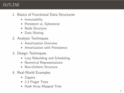
OUTLINE

1. Basics of Functional Data Structures▶ Immutability▶ Persistent vs. Ephemeral▶ Node Structure▶ Data Sharing

2. Analysis Techniques▶ Amortization Overview▶ Amortization with Persistence

3. Design Techniques▶ Lazy Rebuilding and Scheduling▶ Numerical Representations▶ Non-Uniform Structure

4. Real-World Examples▶ Zippers▶ 2-3 Finger Trees▶ Hash Array Mapped Tries

3

MOTIVATION

Functional data structures provide:

▶ Relatively simple implementations▶ Good worst-case performance bounds▶ Persistence for free▶ Ease of use in concurrent programs

4

Basics

5

FUNCTIONAL DATA STRUCTURES?

What do we mean by “Functional Data Structure”?

▶ Built from immutable values▶ Can be implemented in a purely functional language▶ No in-place updates!

Obviously not the data structures taught in Intro to Algorithmsclass…

6

PERSISTENCE

Most imperative structures are ephemeral; updates destroyprevious versionsA data structure is persistent when old versions remain afterupdates

▶ Developed in the context of imperative structures▶ Imperative versions of persistent structures can be quite

complex▶ Adding persistence can change performance bounds▶ Purely functional structures are automatically persistent!

7

VALUE OF PERSISTENCE

Why would we want persistence anyway?

▶ Safe data sharing▶ No locking required▶ Restoration of previous states▶ Interesting algorithms (e.g. in computational geometry)

8

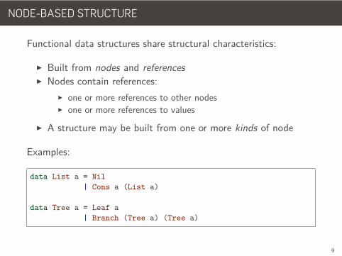
NODE-BASED STRUCTURE

Functional data structures share structural characteristics:

▶ Built from nodes and references▶ Nodes contain references:

▶ one or more references to other nodes▶ one or more references to values

▶ A structure may be built from one or more kinds of node

Examples:

data List a = Nil| Cons a (List a)

data Tree a = Leaf a| Branch (Tree a) (Tree a)

9

DATA SHARING

The fine-grained node structure has some benefits:

▶ New versions of structures share the bulk of their data withold versions

▶ Copying on updates is limited to nodes rather than values▶ Only the nodes on the path from the root to change point are

copied.

Also some drawbacks:

▶ Extra overhead for references vs. in-place storage▶ Locality of data can suffer

10

Analysis

11

Amortization

12

STRUCTURES ENABLE ALGORITHMS

▶ Data structures support operations on them▶ Operations are implemented via algorithms▶ Algorithms perform operations

We bottom out at two primitive operations:

▶ Construction of an ADT value▶ Destructuring/Pattern Matching of an ADT value

13

ALGORITHM COMPARISON

We judge between algorithms based on analysis:

▶ How many primitive operations are needed to complete thealgorithm?

▶ How does the number of operations scale as the problem sizegrows?

Asymptotic analysis gives an upper bound to the growth ofoperation count as the size grows to infinity.

14

WORST CASE

Typical analysis is worst-case:

▶ Find a function such that some constant times that functionof the input size is always greater than the actual count ofoperations for any single operation.

▶ That function is a worst-case upper bound.▶ The smallest upper bound is how we characterize the

asymptotic worst-case behavior.

15

AVERAGE CASE

Sometimes we consider average-case:

▶ Find the upper bounds of all possible single operation cases.▶ Model the statistical likelihood of the cases.▶ Find the smallest upper bound of the weighted combination of

cases.

16

AMORTIZED

An amortized analysis is different:

▶ Find the upper bounds of all possible single operation cases.▶ Consider the possible sequences of operations.▶ Show that expensive operations always run infrequently

enough to distribute their cost among cheap operations

17

WHEN TO AMORTIZE?

A worst-case analysis is necessary when you have hard latencybounds, e.g. real-time requirements.Average or amortized analysis can give a better sense of expectedthroughput of an algorithm.Amortized analysis is useful when most operations are cheap, butoccasionally an expensive one must be performed.Examples:

▶ Array doubling▶ Rehashing▶ Tree balancing

Developed in the context of ephemeral data structures.

18

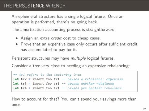
THE PERSISTENCE WRENCH

An ephemeral structure has a single logical future: Once anoperation is performed, there’s no going back.The amortization accounting process is straightforward:

▶ Assign an extra credit cost to cheap cases.▶ Prove that an expensive case only occurs after sufficient credit

has accumulated to pay for it.

Persistent structures may have multiple logical futures.Consider a tree very close to needing an expensive rebalancing:

-- tr1 refers to the teetering treelet tr2 = insert foo tr1 -- causes a rebalance: expensivelet tr3 = insert foo tr1 -- causes another rebalancelet tr4 = insert foo tr1 -- causes yet another rebalance

How to account for that? You can’t spend your savings more thanonce.

19

Functional Amortization

20

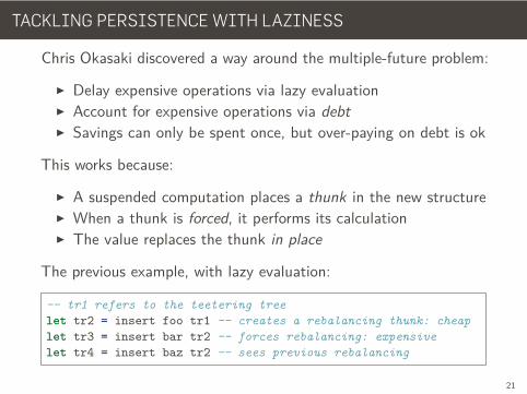
TACKLING PERSISTENCE WITH LAZINESS

Chris Okasaki discovered a way around the multiple-future problem:

▶ Delay expensive operations via lazy evaluation▶ Account for expensive operations via debt▶ Savings can only be spent once, but over-paying on debt is ok

This works because:

▶ A suspended computation places a thunk in the new structure▶ When a thunk is forced, it performs its calculation▶ The value replaces the thunk in place

The previous example, with lazy evaluation:

-- tr1 refers to the teetering treelet tr2 = insert foo tr1 -- creates a rebalancing thunk: cheaplet tr3 = insert bar tr2 -- forces rebalancing: expensivelet tr4 = insert baz tr2 -- sees previous rebalancing

21

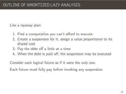
OUTLINE OF AMORTIZED LAZY ANALYSIS

Like a layaway plan:

1. Find a computation you can’t afford to execute2. Create a suspension for it, assign a value proportional to its

shared cost3. Pay the debt off a little at a time4. When the debt is paid off, the suspension may be executed

Consider each logical future as if it were the only one.Each future must fully pay before invoking any suspension.

22

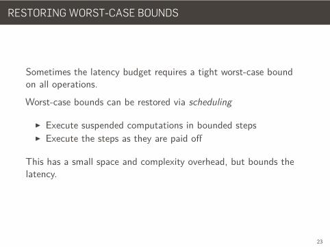
RESTORING WORST-CASE BOUNDS

Sometimes the latency budget requires a tight worst-case boundon all operations.Worst-case bounds can be restored via scheduling

▶ Execute suspended computations in bounded steps▶ Execute the steps as they are paid off

This has a small space and complexity overhead, but bounds thelatency.

23

USING ANALYSIS RESULTS

Sure that sounds like fun, but what’s it good for?Different operations over structures (e.g. head-insert, tail-insert,search) are necessary to implement higher-level algorithms.Choose the data structure that:

▶ Provides good bounds for the operations your algorithm needs▶ Provides the latency guarantees you need

Other factors as well, of course

24

Implementation Patterns

25

Lazy Rebuilding

26

QUEUES, TAKE 1

The essence of the Queue:

▶ insert adds an element at the end of the queue▶ remove takes an element from the front of the queue

How to represent it? What about a List?

▶ Our remove operation is O (1)▶ But insert is O (n)!

The standard trick: A pair of lists, left and right.

▶ The left list holds the head of the queue▶ The right list holds the tail, stored in reversed order

When left becomes empty, reverse right and put it in left.

27

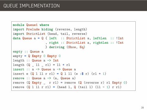
QUEUE IMPLEMENTATION

module Queue1 whereimport Prelude hiding (reverse, length)import StrictList (head, tail, reverse)data Queue a = Q { left :: StrictList a, leftLen :: !Int

, right :: StrictList a, rightLen :: !Int} deriving (Show, Eq)

empty :: Queue aempty = Q Empty 0 Empty 0length :: Queue a -> Intlength (Q _ ll _ rl) = ll + rlinsert :: a -> Queue a -> Queue ainsert e (Q l ll r rl) = Q l ll (e :$ r) (rl + 1)remove :: Queue a -> (a, Queue a)remove (Q Empty _ r rl) = remove (Q (reverse r) rl Empty 0)remove (Q l ll r rl) = (head l, Q (tail l) (ll - 1) r rl)

28

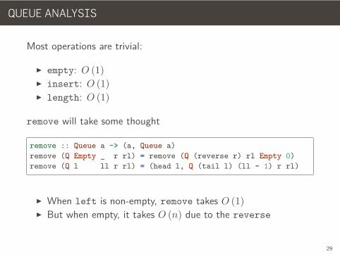
QUEUE ANALYSIS

Most operations are trivial:

▶ empty: O (1)▶ insert: O (1)▶ length: O (1)

remove will take some thought

remove :: Queue a -> (a, Queue a)remove (Q Empty _ r rl) = remove (Q (reverse r) rl Empty 0)remove (Q l ll r rl) = (head l, Q (tail l) (ll - 1) r rl)

▶ When left is non-empty, remove takes O (1)▶ But when empty, it takes O (n) due to the reverse

29

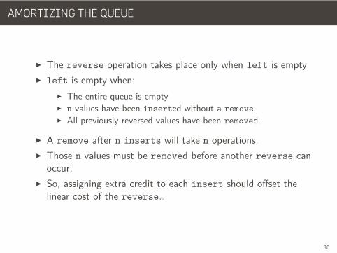
AMORTIZING THE QUEUE

▶ The reverse operation takes place only when left is empty▶ left is empty when:

▶ The entire queue is empty▶ n values have been inserted without a remove▶ All previously reversed values have been removed.

▶ A remove after n inserts will take n operations.▶ Those n values must be removed before another reverse can

occur.▶ So, assigning extra credit to each insert should offset the

linear cost of the reverse…

30

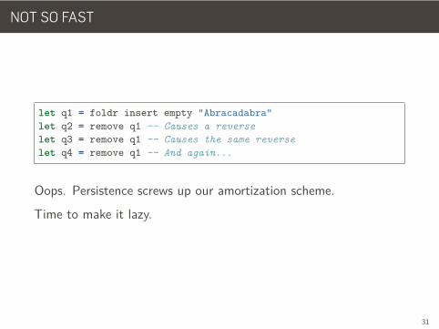
NOT SO FAST

let q1 = foldr insert empty "Abracadabra"let q2 = remove q1 -- Causes a reverselet q3 = remove q1 -- Causes the same reverselet q4 = remove q1 -- And again...

Oops. Persistence screws up our amortization scheme.Time to make it lazy.

31

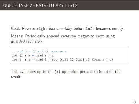
QUEUE TAKE 2 - PAIRED LAZY LISTS

Goal: Reverse right incrementally before left becomes empty.Means: Periodically append reverse right to left usingguarded recursion.

-- rot l r [] = l ++ reverse rrot [] r a = head r : arot l r a = head l : rot (tail l) (tail r) (head r : a)

This evaluates up to the (:) operation per call to head on theresult.

32

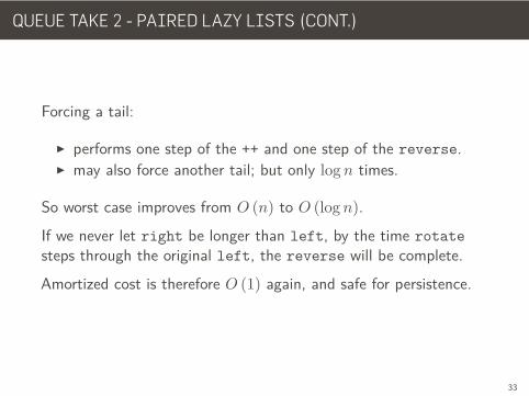
QUEUE TAKE 2 - PAIRED LAZY LISTS (CONT.)

Forcing a tail:

▶ performs one step of the ++ and one step of the reverse.▶ may also force another tail; but only log n times.

So worst case improves from O (n) to O (log n).If we never let right be longer than left, by the time rotatesteps through the original left, the reverse will be complete.Amortized cost is therefore O (1) again, and safe for persistence.

33

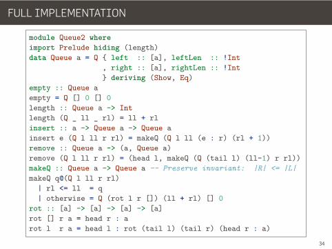
FULL IMPLEMENTATION

module Queue2 whereimport Prelude hiding (length)data Queue a = Q { left :: [a], leftLen :: !Int

, right :: [a], rightLen :: !Int} deriving (Show, Eq)

empty :: Queue aempty = Q [] 0 [] 0length :: Queue a -> Intlength (Q _ ll _ rl) = ll + rlinsert :: a -> Queue a -> Queue ainsert e (Q l ll r rl) = makeQ (Q l ll (e : r) (rl + 1))remove :: Queue a -> (a, Queue a)remove (Q l ll r rl) = (head l, makeQ (Q (tail l) (ll-1) r rl))makeQ :: Queue a -> Queue a -- Preserve invariant: |R| <= |L|makeQ q@(Q l ll r rl)

| rl <= ll = q| otherwise = Q (rot l r []) (ll + rl) [] 0

rot :: [a] -> [a] -> [a] -> [a]rot [] r a = head r : arot l r a = head l : rot (tail l) (tail r) (head r : a)

34

Numerical Representations

35

ARITHMETIC

Many people regard arithmetic as a trivial thing thatchildren learn and computers do, but we will see thatarithmetic is a fascinating topic with many interestingfacets. It is important to make a thorough study ofefficient methods for calculating with numbers, sincearithmetic underlies so many computer applications.

Donald E. Knuth, from “The Art of Computer Programming”

36

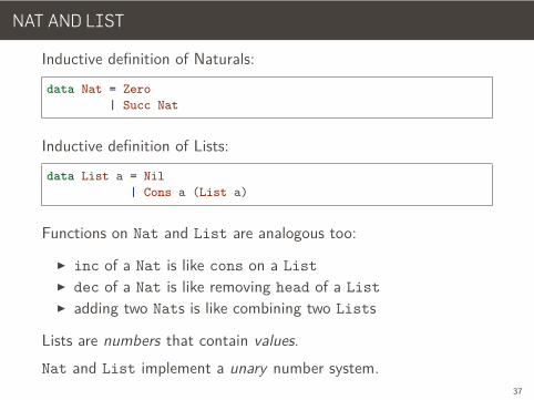
NAT AND LIST

Inductive definition of Naturals:data Nat = Zero

| Succ Nat

Inductive definition of Lists:data List a = Nil

| Cons a (List a)

Functions on Nat and List are analogous too:

▶ inc of a Nat is like cons on a List▶ dec of a Nat is like removing head of a List▶ adding two Nats is like combining two Lists

Lists are numbers that contain values.Nat and List implement a unary number system.

37

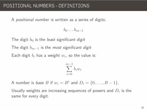
POSITIONAL NUMBERS - DEFINITIONS

A positional number is written as a series of digits:

b0 . . . bm−1

The digit b0 is the least significant digitThe digit bm−1 is the most significant digitEach digit bi has a weight wi, so the value is:

m−1∑i=0

biwi

A number is base B if wi = Bi and Di = {0, . . . , B − 1}.Usually weights are increasing sequences of powers and Di is thesame for every digit.

38

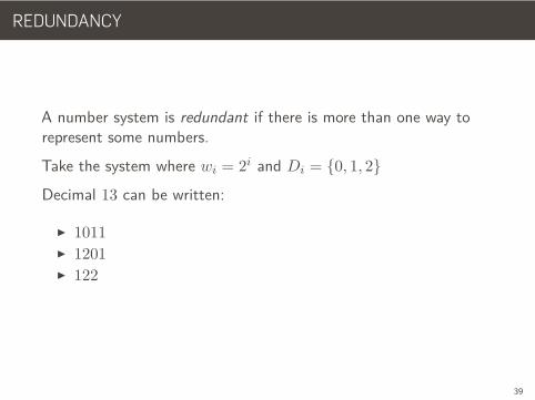
REDUNDANCY

A number system is redundant if there is more than one way torepresent some numbers.Take the system where wi = 2i and Di = {0, 1, 2}

Decimal 13 can be written:

▶ 1011▶ 1201▶ 122

39

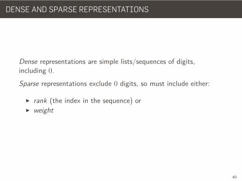
DENSE AND SPARSE REPRESENTATIONS

Dense representations are simple lists/sequences of digits,including 0.Sparse representations exclude 0 digits, so must include either:

▶ rank (the index in the sequence) or▶ weight

40

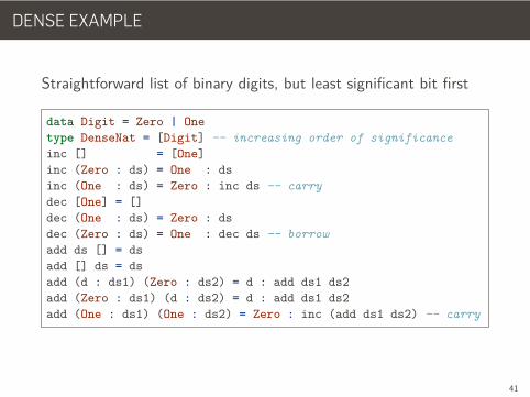
DENSE EXAMPLE

Straightforward list of binary digits, but least significant bit first

data Digit = Zero | Onetype DenseNat = [Digit] -- increasing order of significanceinc [] = [One]inc (Zero : ds) = One : dsinc (One : ds) = Zero : inc ds -- carrydec [One] = []dec (One : ds) = Zero : dsdec (Zero : ds) = One : dec ds -- borrowadd ds [] = dsadd [] ds = dsadd (d : ds1) (Zero : ds2) = d : add ds1 ds2add (Zero : ds1) (d : ds2) = d : add ds1 ds2add (One : ds1) (One : ds2) = Zero : inc (add ds1 ds2) -- carry

41

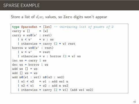
SPARSE EXAMPLE

Store a list of diwi values, so Zero digits won’t appear

type SparseNat = [Int] -- increasing list of powers of 2carry w [] = [w]carry w ws@(w' : rest)

| w < w' = w : ws| otherwise = carry (2 * w) rest

borrow w ws@(w' : rest)| w < w' = rest| otherwise = w : borrow (2 * w) ws

inc ws = carry 1 wsdec ws = borrow 1 wsadd ws [] = wsadd [] ws = wsadd m@(w1 : ws1) n@(w2 : ws2)

| w1 < w2 = w1 : add ws1 n| w2 < w1 = w2 : add m ws2| otherwise = carry (2 * w1) (add ws1 ws2)

42

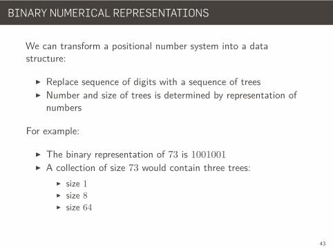
BINARY NUMERICAL REPRESENTATIONS

We can transform a positional number system into a datastructure:

▶ Replace sequence of digits with a sequence of trees▶ Number and size of trees is determined by representation of

numbers

For example:

▶ The binary representation of 73 is 1001001▶ A collection of size 73 would contain three trees:

▶ size 1▶ size 8▶ size 64

43

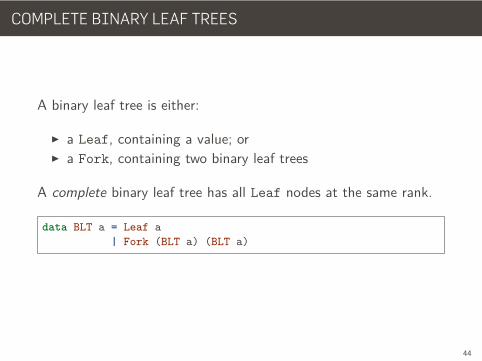
COMPLETE BINARY LEAF TREES

A binary leaf tree is either:

▶ a Leaf, containing a value; or▶ a Fork, containing two binary leaf trees

A complete binary leaf tree has all Leaf nodes at the same rank.

data BLT a = Leaf a| Fork (BLT a) (BLT a)

44

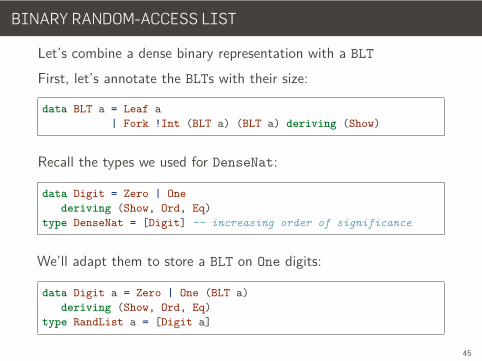
BINARY RANDOM-ACCESS LIST

Let’s combine a dense binary representation with a BLT

First, let’s annotate the BLTs with their size:

data BLT a = Leaf a| Fork !Int (BLT a) (BLT a) deriving (Show)

Recall the types we used for DenseNat:

data Digit = Zero | Onederiving (Show, Ord, Eq)

type DenseNat = [Digit] -- increasing order of significance

We’ll adapt them to store a BLT on One digits:

data Digit a = Zero | One (BLT a)deriving (Show, Ord, Eq)

type RandList a = [Digit a]

45

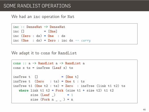
SOME RANDLIST OPERATIONS

We had an inc operation for Nat

inc :: DenseNat -> DenseNatinc [] = [One]inc (Zero : ds) = One : dsinc (One : ds) = Zero : inc ds -- carry

We adapt it to cons for RandList

cons :: a -> RandList a -> RandList acons x ts = insTree (Leaf x) ts

insTree t [] = [One t]insTree t (Zero : ts) = One t : tsinsTree t1 (One t2 : ts) = Zero : insTree (link t1 t2) ts

where link t1 t2 = Fork (size t1 + size t2) t1 t2size (Leaf _) = 1size (Fork n _ _ ) = n

46

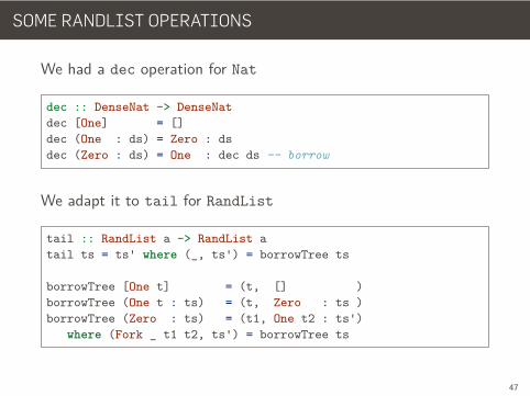
SOME RANDLIST OPERATIONS

We had a dec operation for Nat

dec :: DenseNat -> DenseNatdec [One] = []dec (One : ds) = Zero : dsdec (Zero : ds) = One : dec ds -- borrow

We adapt it to tail for RandList

tail :: RandList a -> RandList atail ts = ts' where (_, ts') = borrowTree ts

borrowTree [One t] = (t, [] )borrowTree (One t : ts) = (t, Zero : ts )borrowTree (Zero : ts) = (t1, One t2 : ts')

where (Fork _ t1 t2, ts') = borrowTree ts

47

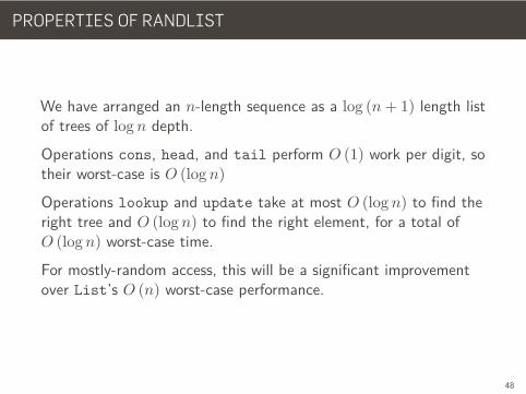
PROPERTIES OF RANDLIST

We have arranged an n-length sequence as a log (n + 1) length listof trees of log n depth.Operations cons, head, and tail perform O (1) work per digit, sotheir worst-case is O (log n)

Operations lookup and update take at most O (log n) to find theright tree and O (log n) to find the right element, for a total ofO (log n) worst-case time.For mostly-random access, this will be a significant improvementover List’s O (n) worst-case performance.

48

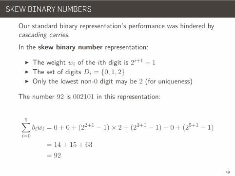
SKEW BINARY NUMBERS

Our standard binary representation’s performance was hindered bycascading carries.In the skew binary number representation:

▶ The weight wi of the ith digit is 2i+1 − 1▶ The set of digits Di = {0, 1, 2}▶ Only the lowest non-0 digit may be 2 (for uniqueness)

The number 92 is 002101 in this representation:

5∑i=0

biwi = 0 + 0 + (22+1 − 1) × 2 + (23+1 − 1) + 0 + (25+1 − 1)

= 14 + 15 + 63= 92

49

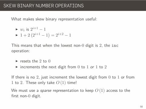
SKEW BINARY NUMBER OPERATIONS

What makes skew binary representation useful:

▶ wi is 2i+1 − 1▶ 1 + 2

(2i+1 − 1

)= 2i+2 − 1

This means that when the lowest non-0 digit is 2, the incoperation:

▶ resets the 2 to 0▶ increments the next digit from 0 to 1 or 1 to 2

If there is no 2, just increment the lowest digit from 0 to 1 or from1 to 2. These only take O (1) time!We must use a sparse representation to keep O (1) access to thefirst non-0 digit.

50

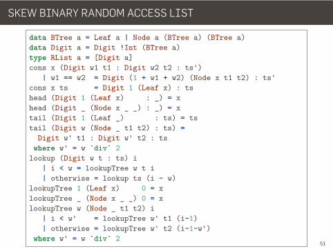
SKEW BINARY RANDOM ACCESS LIST

data BTree a = Leaf a | Node a (BTree a) (BTree a)data Digit a = Digit !Int (BTree a)type RList a = [Digit a]cons x (Digit w1 t1 : Digit w2 t2 : ts')

| w1 == w2 = Digit (1 + w1 + w2) (Node x t1 t2) : ts'cons x ts = Digit 1 (Leaf x) : tshead (Digit 1 (Leaf x) : _) = xhead (Digit _ (Node x _ _) : _) = xtail (Digit 1 (Leaf _) : ts) = tstail (Digit w (Node _ t1 t2) : ts) =

Digit w' t1 : Digit w' t2 : tswhere w' = w `div` 2

lookup (Digit w t : ts) i| i < w = lookupTree w t i| otherwise = lookup ts (i - w)

lookupTree 1 (Leaf x) 0 = xlookupTree _ (Node x _ _) 0 = xlookupTree w (Node _ t1 t2) i

| i < w' = lookupTree w' t1 (i-1)| otherwise = lookupTree w' t2 (i-1-w')

where w' = w `div` 251

Non-Uniform Structure

52

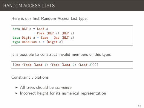
RANDOM ACCESS LISTS

Here is our first Random Access List type:

data BLT a = Leaf a| Fork (BLT a) (BLT a)

data Digit a = Zero | One (BLT a)type RandList a = [Digit a]

It is possible to construct invalid members of this type:

[One (Fork (Leaf 1) (Fork (Leaf 2) (Leaf 3)))]

Constraint violations:

▶ All trees should be complete▶ Incorrect height for its numerical representation

53

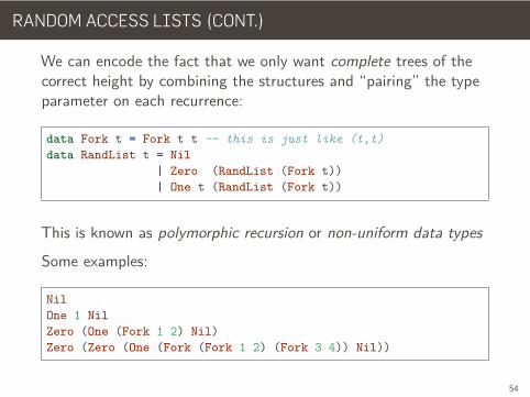
RANDOM ACCESS LISTS (CONT.)

We can encode the fact that we only want complete trees of thecorrect height by combining the structures and “pairing” the typeparameter on each recurrence:

data Fork t = Fork t t -- this is just like (t,t)data RandList t = Nil

| Zero (RandList (Fork t))| One t (RandList (Fork t))

This is known as polymorphic recursion or non-uniform data typesSome examples:

NilOne 1 NilZero (One (Fork 1 2) Nil)Zero (Zero (One (Fork (Fork 1 2) (Fork 3 4)) Nil))

54

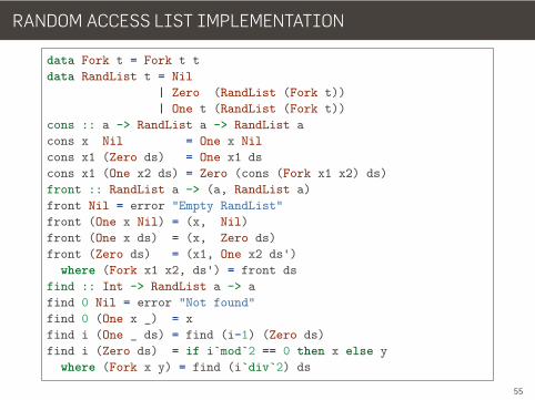
RANDOM ACCESS LIST IMPLEMENTATION

data Fork t = Fork t tdata RandList t = Nil

| Zero (RandList (Fork t))| One t (RandList (Fork t))

cons :: a -> RandList a -> RandList acons x Nil = One x Nilcons x1 (Zero ds) = One x1 dscons x1 (One x2 ds) = Zero (cons (Fork x1 x2) ds)front :: RandList a -> (a, RandList a)front Nil = error "Empty RandList"front (One x Nil) = (x, Nil)front (One x ds) = (x, Zero ds)front (Zero ds) = (x1, One x2 ds')

where (Fork x1 x2, ds') = front dsfind :: Int -> RandList a -> afind 0 Nil = error "Not found"find 0 (One x _) = xfind i (One _ ds) = find (i-1) (Zero ds)find i (Zero ds) = if i`mod`2 == 0 then x else y

where (Fork x y) = find (i`div`2) ds

55

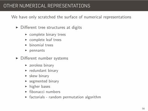
OTHER NUMERICAL REPRESENTATIONS

We have only scratched the surface of numerical representations

▶ Different tree structures at digits▶ complete binary trees▶ complete leaf trees▶ binomial trees▶ pennants

▶ Different number systems▶ zeroless binary▶ redundant binary▶ skew binary▶ segmented binary▶ higher bases▶ fibonacci numbers▶ factorials - random permutation algorithm

56

Real-World Structures

57

Zippers

58

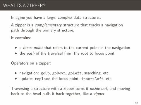
WHAT IS A ZIPPER?

Imagine you have a large, complex data structure…A zipper is a complementary structure that tracks a navigationpath through the primary structure.It contains:

▶ a focus point that refers to the current point in the navigation▶ the path of the traversal from the root to focus point

Operators on a zipper:

▶ navigation: goUp, goDown, goLeft, searching, etc.▶ update: replace the focus point, insertLeft, etc.

Traversing a structure with a zipper turns it inside-out, and movingback to the head pulls it back together, like a zipper.

59

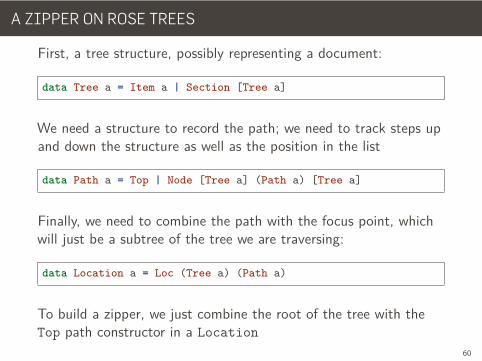
A ZIPPER ON ROSE TREES

First, a tree structure, possibly representing a document:

data Tree a = Item a | Section [Tree a]

We need a structure to record the path; we need to track steps upand down the structure as well as the position in the list

data Path a = Top | Node [Tree a] (Path a) [Tree a]

Finally, we need to combine the path with the focus point, whichwill just be a subtree of the tree we are traversing:

data Location a = Loc (Tree a) (Path a)

To build a zipper, we just combine the root of the tree with theTop path constructor in a Location

60

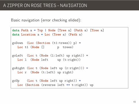
A ZIPPER ON ROSE TREES - NAVIGATION

Basic navigation (error checking elided):

data Path a = Top | Node [Tree a] (Path a) [Tree a]data Location a = Loc (Tree a) (Path a)

goDown (Loc (Section (t1:trees)) p) =Loc t1 (Node [] p trees)

goLeft (Loc t (Node (l:left) up right)) =Loc l (Node left up (t:right))

goRight (Loc t (Node left up (r:right))) =Loc r (Node (t:left) up right)

goUp (Loc t (Node left up right)) =Loc (Section (reverse left ++ t:right)) up

61

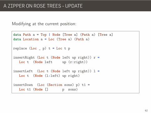
A ZIPPER ON ROSE TREES - UPDATE

Modifying at the current position:

data Path a = Top | Node [Tree a] (Path a) [Tree a]data Location a = Loc (Tree a) (Path a)

replace (Loc _ p) t = Loc t p

insertRight (Loc t (Node left up right)) r =Loc t (Node left up (r:right))

insertLeft (Loc t (Node left up right)) l =Loc t (Node (l:left) up right)

insertDown (Loc (Section sons) p) t1 =Loc t1 (Node [] p sons)

62

CRAZY ZIPPER FACTS

The zipper structure for a given data structure can be derivedmechanically from its algebraic type signature.The zipper type signature is the first derivative (in the sense youlearned in Calculus) of its parent signature.Zippers are one-hole contexts for their parent type. The focuspoint is the hole.Zippers can also be represented by delimited continuations of atraversing process. These can be used with any Traversablewithout knowing its concrete type at all!Continuation-capturing traversal functions invert the controlstructure in a similar manner to how taking the derivative of thedata type inverts its data structure.

63

2-3 Finger Trees

64

NOT THIS TIME

I lied. There’s no time to talk about these. Sorry!But you should be prepared to read this paper about them now:http://www.cs.ox.ac.uk/people/ralf.hinze/publications/FingerTrees.pdf

65

Hash Array Mapped Tries

66

DOWNSIDES TO THIS STUFF

Way back at the beginning, I mentioned some downsides:

▶ Extra overhead for references vs. in-place storage▶ Locality of data can suffer

These are constant-factor issues, but with the advances in thecache structure of machines, they are an increasingly largeconstant factor.Bad memory access patterns can make memory fetches take ordersof magnitude longer.The solution is to use bigger chunks of data; do more copying andless pointer chasing.

67

HASH ARRAY MAPPED TRIE

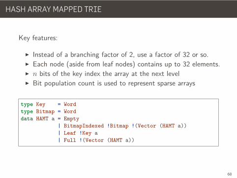
Key features:

▶ Instead of a branching factor of 2, use a factor of 32 or so.▶ Each node (aside from leaf nodes) contains up to 32 elements.▶ n bits of the key index the array at the next level▶ Bit population count is used to represent sparse arrays

type Key = Wordtype Bitmap = Worddata HAMT a = Empty

| BitmapIndexed !Bitmap !(Vector (HAMT a))| Leaf !Key a| Full !(Vector (HAMT a))

68

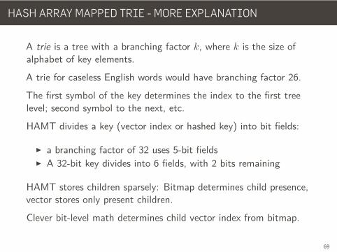
HASH ARRAY MAPPED TRIE - MORE EXPLANATION

A trie is a tree with a branching factor k, where k is the size ofalphabet of key elements.A trie for caseless English words would have branching factor 26.The first symbol of the key determines the index to the first treelevel; second symbol to the next, etc.HAMT divides a key (vector index or hashed key) into bit fields:

▶ a branching factor of 32 uses 5-bit fields▶ A 32-bit key divides into 6 fields, with 2 bits remaining

HAMT stores children sparsely: Bitmap determines child presence,vector stores only present children.Clever bit-level math determines child vector index from bitmap.

69

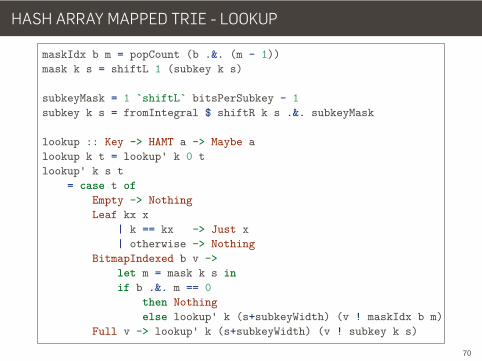
HASH ARRAY MAPPED TRIE - LOOKUP

maskIdx b m = popCount (b .&. (m - 1))mask k s = shiftL 1 (subkey k s)

subkeyMask = 1 `shiftL` bitsPerSubkey - 1subkey k s = fromIntegral $ shiftR k s .&. subkeyMask

lookup :: Key -> HAMT a -> Maybe alookup k t = lookup' k 0 tlookup' k s t

= case t ofEmpty -> NothingLeaf kx x

| k == kx -> Just x| otherwise -> Nothing

BitmapIndexed b v ->let m = mask k s inif b .&. m == 0

then Nothingelse lookup' k (s+subkeyWidth) (v ! maskIdx b m)

Full v -> lookup' k (s+subkeyWidth) (v ! subkey k s)

70

Conclusion

71

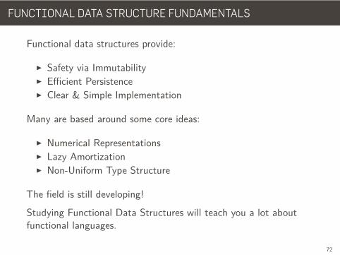
FUNCTIONAL DATA STRUCTURE FUNDAMENTALS

Functional data structures provide:

▶ Safety via Immutability▶ Efficient Persistence▶ Clear & Simple Implementation

Many are based around some core ideas:

▶ Numerical Representations▶ Lazy Amortization▶ Non-Uniform Type Structure

The field is still developing!Studying Functional Data Structures will teach you a lot aboutfunctional languages.

72