Full First-Order Sequent and Tableau Calculi With ... · will use nullary parameters, which we call...
42
arXiv:0902.3730v1 [cs.AI] 21 Feb 2009 Full First-Order Sequent and Tableau Calculi With Preservation of Solutions and the Liberalized δ -Rule but Without Skolemization Claus-Peter Wirth [email protected] http://www.ags.uni-sb.de/ ˜ cp Research Report 698/1998 http://www.ags.uni-sb.de/ ˜ cp/p/ftp98/long.html December 13, 1998 Revised April 1, 1999 (Typos corrected, Proof of Lemma 5.4 and Abstract shortened, References extended) Revised Sept. 29, 1999 (Typos corrected) Searchable Online Edition Universit¨ at Dortmund Informatik V D-44221 Dortmund Germany Abstract: We present a combination of raising, explicit variable dependency representation, the liberalized δ- rule, and preservation of solutions for first-order deductive theorem proving. Our main motivation is to provide the foundation for our work on inductive theorem proving.
Transcript of Full First-Order Sequent and Tableau Calculi With ... · will use nullary parameters, which we call...
arX
iv:0
902.
3730
v1 [
cs.A
I] 2
1 F
eb 2
009
Full First-Order Sequent and Tableau Calculi WithPreservation of Solutions
and the Liberalized δ-Rule butWithout Skolemization
Claus-Peter Wirth
http://www.ags.uni-sb.de/˜cp
Research Report 698/1998http://www.ags.uni-sb.de/˜cp/p/ftp98/long.html
December 13, 1998
Revised April 1, 1999(Typos corrected, Proof of Lemma 5.4 and Abstract shortened, References extended)
Revised Sept. 29, 1999(Typos corrected)
Searchable Online Edition
Universitat DortmundInformatik V
D-44221 DortmundGermany
Abstract: We present a combination of raising, explicit variable dependency representation, the liberalizedδ-rule, and preservation of solutions for first-order deductive theorem proving. Our main motivation is to provide thefoundation for our work on inductive theorem proving.
Contents
1 Introduction 1
1.1 Without Skolemization . . . . . . . . . . . . . . . . . . . . . . . . . . . .. 1
1.2 Sequent and Tableau Calculi . . . . . . . . . . . . . . . . . . . . . . . .. . 3
1.3 Preservation of Solutions . . . . . . . . . . . . . . . . . . . . . . . . .. . . 4
1.4 The Liberalizedδ-rule . . . . . . . . . . . . . . . . . . . . . . . . . . . . . 5
2 Basic Notions, Notations, and Assumptions 8
3 Two Versions of Variable-Conditions 9
4 The Weak Version 12
5 The Strong Version 17
6 Conclusion 28
7 The Proofs 29
1
1 Introduction
The paper organizes as follows: After explaining the technical terms of the title in§ 1 and theremaining basic notions in§ 2, we start to explicate the differences between our two versions ofcalculi in§ 3. The weak version is explained in§4. The changes necessary for the strong versionin order to admit liberalization of theδ-rule are explained in§ 5. After concluding in§6 weappend all the proofs, references, and notes.
1.1 Without Skolemization
In this paper we discuss how to analytically prove first-order theorems in contexts where Skolem-ization is not appropriate. Skolemization has at least three problematic aspects.
1. Skolemization enrichs the signature or introduces higher-order variables. Unless specialcare is taken, this may introduce objects into empty universes and change the notion ofterm-generatedness or Herbrand models. Above that, the Skolem functions occur in an-swers to goals or solutions of constraints1 which in general cannot be translated into theoriginal signature. For a detailed discussion of these problems cf. Miller (1992).
2. Skolemization results in the following simplified quantification structure:
For all Skolem functions~u there are solutions to the freeγ-variables~e (i.e. thefree variables of Fitting (1996)) such that the quantifier-free theoremT (~e, ~u) isvalid.Short: ∀~u. ∃~e. T (~e, ~u).
Since the state of a proof attempt is often represented as theconjunction of the branchesof a tree (e.g. in sequent or (dual) tableau calculi), the free γ-variables become “rigid” or“global”, i.e. a solution for a freeγ-variable must solve all occurrences of this variable inthe whole proof tree. This is because, forB0, . . . , Bn denoting the branches of the prooftree,
∀~u. ∃~e. ( B0 ∧ . . . ∧ Bn )
is logically strictly stronger than∀~u. ( ∃~e. B0 ∧ . . . ∧ ∃~e. Bn ).
2
Moreover, with this quantification structure it does not seem to be possible to do inductivetheorem proving by finding, for each assumed counterexample, another counterexamplethat is strictly smaller in some wellfounded ordering.2 The reason for this is the following.When we have some counterexample~u for T (~e, ~u) (i.e. there is no~e such thatT (~e, ~u) isvalid) then for different~e different branchesBi in the proof tree may cause the invalidityof the conjunction. If we have applied induction hypothesesin more than one branch, fordifferent~e we get different smaller counterexamples. What we would need, however, is onesingle smaller counterexample for all~e.
3. Skolemization increases the size of the formulas. (Note that in most calculi the only relevantpart of Skolem terms is the top symbol and the set of occurringvariables.)
The first and second problematic aspects disappear when one usesraising (cf. Miller (1992))instead of Skolemization. Raising is a dual of Skolemization and simplifies the quantificationstructure to something like:
There are raising functions~e such that for all possible values of the freeδ-vari-ables~u (i.e. the nullary constants or “parameters”) the quantifier-free theoremT (~e, ~u)is valid.Short: ∃~e. ∀~u. T (~e, ~u).
Note that due to the two duality switches “unsatisfiability/validity” and “Skolemization/raising”, in this paper raising will look much like Skolemization in refutational theorem proving.The inverted order of universal and existential quantification of raising (compared to Skolemiza-tion) is advantageous because now
∃~e. ∀~u. ( B0 ∧ . . . ∧ Bn )
is indeed logically equivalent to∃~e. ( ∀~u. B0 ∧ . . . ∧ ∀~u. Bn ).
Furthermore, inductive theorem proving works well: When, for some~e, we have some counter-example~u for T (~e, ~u) (i.e. T (~e, ~u) is invalid) then one branchBi in the proof tree must causethe invalidity of the conjunction. If this branch is closed,then it contains the application of aninduction hypothesis that is invalid for this~e and the~u′ resulting from the instantiation of thehypothesis. Thus,~u′ together with the induction hypothesis provides the strictly smaller counter-example we are searching for for this~e.
The third problematic aspect disappears when the dependency of variables is explicitly rep-resented in avariable-condition, cf. Kohlhase (1995). This idea actually has a long history,cf.Prawitz (1960), Kanger (1963), Bibel (1987). Moreover, theuse of variable-conditions admits thefree existential variables to be first-order.
3
1.2 Sequent and Tableau Calculi
In Smullyan (1968), rules for analytic theorem proving are classified asα-, β-, γ-, andδ-rulesindependently from a concrete calculus.
α-rules describe the simple and the
β-rules the case-splitting propositional proof steps.
γ-rules show existential properties, either by exhibiting a term witnessing to the existence or elseby introducing a special kind of variable, called “dummy” inPrawitz (1960) and Kanger(1963), and “free variable” in footnote 11 of Prawitz (1960)and in Fitting (1996). We willcall these variablesfreeγ-variables. By the use of freeγ-variables we can delay the choiceof a witnessing term until the state of the proof attempt gives us more information whichchoice is likely to result in a successful proof. It is the important addition of freeγ-vari-ables that makes the major difference between the free variable calculi of Fitting (1996) andthe calculi of Smullyan (1968). Since there use to be infinitely many possibly witnessingterms (and different branches may need different ones), theγ-rules (under assistance of theβ-rules) often destroy the possibility to decide validity because they enable infinitely manyγ-rule applications to the same formula.
δ-rules show universal properties simply with the help of a new symbol, called a “parameter”,about which nothing is known. Since the present freeγ-variables must not be instantiatedwith this new parameter, in the standard framework of Skolemization and unification theparameter is given the present freeγ-variables as arguments. In this paper, however, wewill use nullary parameters, which we callfreeδ-variables. These variables are not free inthe sense that they may be chosen freely, but in the sense thatthey are not bound by anyquantifier. Our freeδ-variables are similar to the parameters of Kanger (1963) because afreeγ-variable may not be instantiated with all of them. We will store the information onthe dependency between freeγ-variables and freeδ-variables invariable-conditions.
4
1.3 Preservation of Solutions
Users even of pure Prolog are not so much interested in theorem proving as they are in answercomputation. The theorem they want to prove usually contains some free existential variablesthat are instantiated during a proof attempt. When the proofattempt is successful, not only theinput theorem is known to be valid but also the instance of thetheorem with the substitutionbuilt-up during the proof. Since the knowledge of mere existence is much less useful than theknowledge of a term that witnesses to this existence (unlessthis term is a only free existentialvariable), theorem proving should—if possible—always provide these witnessing terms. Answercomputation is no problem in Prolog’s Horn logic because it is so simple. But also for the moredifficult clausal logic, answer computation is possible. Cf. e.g. Baumgartner &al. (1997), wheretableau calculi are used for answer computation in clausal logic. Answer computation becomeseven harder when we consider full first-order logic instead of clausal logic. Whenδ-steps occurin a proof, the introduced free universal variables may provide no information on what kind ofobject they denote. Their excuse may be that they cannot do this in terms of computability orλ-terms. Nevertheless, they can provide this information inform of Hilbert’s ε-terms, and thestrong versions of our calculi will do so. When full first-order logic is considered, one shouldfocus onpreservation of solutionsinstead of computing answers. By this we mean at least thefollowing property:
All solutions that transform a proof attempt for a proposition into a closed proof (i.e.the closing substitutions for the freeγ-variables) are also solutions of the originalproposition.
This again is closely related to inductive theorem proving:Suppose that we finally have shownthat for the reduced formR(~e, ~u) (i.e. the state of the proof attempt) of the original theoremT (~e, ~u) (cf. the discussion in§ 1.1), there is some solution~e such that for each counterexample~uof R(~e, ~u) there is a counterexample~u′ for the original theorem and that this~u′ is strictly smallerthan~u in some wellfounded ordering. In this case we have provedT (~e, ~u) only if the solution~efor the reduced form∀~u. R(~e, ~u) is also a solution for the original theorem∀~u. T (~e, ~u).
5
1.4 The Liberalizedδ-rule
We use ‘⊎’ for the union of disjoint classes and ‘id’ for the identity function. For a classR wedefinedomain, range, andrestriction toandimage3 andreverse-image of a classA by
dom(R) := {a | ∃b. (a, b)∈R} ;ran(R) := {b | ∃a. (a, b)∈R} ;
A↿R := {(a, b)∈R | a∈A} ;〈A〉R := {b | ∃a∈A. (a, b)∈R} ;R〈B〉 := {a | ∃b∈B. (a, b)∈R} .
We define asequentto be a list of formulas.4 Theconjugateof a formulaA (written: A ) is theformulaB if A is of the form¬B, and the formula¬A otherwise. Note that the conjugate of theconjugate of a formula is the original formula again, unlessit has the form¬¬B.
In the tradition of Gentzen (1935) we assume the symbols forfreeγ-variables(i.e. the freevariables of Fitting (1996)),freeδ-variables(i.e. nullary parameters),bound variables(i.e. vari-ables for quantified use only), and theconstants(i.e. the function (and predicate) symbols fromthe signature) to come from four disjoint setsVγ, Vδ, Vbound, andΣ. We assume each ofVγ, Vδ,Vbound to be infinite (for each sort) and setVfree := Vγ⊎Vδ. Moreover, due to the possibility torename bound variables w.l.o.g., we do not permit quantification on variables that occur alreadybound in a formula; i.e. e.g.∀x:A is only a formula in our sense ifA does not contain a quantifieronx like ∀x or∃x. The simple effect is that ourγ- andδ-rules can simply replaceall occurrencesof x. For a term, formula, sequentΓ &c., ‘Vγ(Γ )’, ‘ Vδ(Γ )’, ‘ Vbound(Γ )’, ‘ Vfree(Γ )’ denote the setsof variables fromVγ, Vδ, Vbound, Vfree occurring inΓ , resp.. For a substitutionσ we denote with‘Γσ’ the result of replacing inΓ each variablex in dom(σ) with σ(x). Unless stated otherwise,we tacitly assume that each substitutionσ satisfiesVbound(dom(σ) ∪ ran(σ)) = ∅, such that nobound variables can be replaced and no additional variablesbecome bound (i.e. captured) whenapplyingσ.
A variable-conditionR is a subset ofVγ × Vδ. Roughly speaking,(xγ, yδ)∈R says thatxγ isolder thanyδ, so that we must not instantiate the freeγ-variablexγ with a term containingyδ.
While the benefit of the introduction of freeγ-variables inγ-rules is to delay the choice ofa witnessing term, it is sometimes unsound to instantiate such a freeγ-variablexγ with a termcontaining a freeδ-variableyδ that was introduced later thanxγ:
6
Example 1.1∃x. ∀y. (x= y)
is not deductively valid. We can start a proof attempt via:γ-step:
∀y. (xγ= y).δ-step:
(xγ= yδ).
Now, if we were allowed to substitute the freeγ-variablexγ with the freeδ-variableyδ, we wouldget the tautology(yδ= yδ), i.e. we would have proved an invalid formula. In order to preventthis, theδ-step has to record(xγ, yδ) in the variable-condition, which disallows the instantiationstep.
In order to restrict the possible instantiations as little as possible, we should keep our variable-conditions as small as possible. Kanger (1963) and Bibel (1987) are quite generous in that theylet their variable-conditions become quite big:
Example 1.2∃x.
(
P(x) ∨ ∀y. ¬P(y))
can be proved the following way:γ-step:
(
P(xγ) ∨ ∀y. ¬P(y))
.α-step:
P(xγ), ∀y. ¬P(y).δ-step:
P(xγ), ¬P(yδ).Instantiation step:
P(yδ), ¬P(yδ).
The last step is not allowed in the above citations, so that anotherγ-step must be applied to theoriginal formula in order to prove it. Our instantiation step, however, is perfectly sound: Sincexγ
does not occur in∀y. ¬P(y), the free variablesxγ andyδ do not depend on each other and thereis no reason to insist onxγ being older thanyδ. Note that moving-in the existential quantifiertransforms the original formula into the logically equivalent formula ∃x. P(x) ∨ ∀y. ¬P(y),which (after a precedingα-step) enables theδ-step introducingyδ to come before theγ-stepintroducingxγ.
Keeping small the variable-conditions generated by theδ-rule results in non-elementary reduc-tion of the size of smallest proofs. This “liberalization oftheδ-rule” has a history ranging fromSmullyan (1968) over Hahnle & Schmitt (1994) to Baaz & Ferm¨uller (1995). While the liberal-izedδ-rule of Smullyan (1968) is already able to prove the formulaof Example 1.2 with a singleγ-step, it is much more restrictive than the more liberalizedδ-rule of Baaz & Fermuller (1995).
7
Note that liberalization of theδ-rule is not simple because it easily results in unsound calculi,cf. Kohlhase (1995) w.r.t. our Example 1.3 and Kohlhase (1998) w.r.t. our Example 5.18. Thedifficulty lies with instantiation steps that relate previously unrelated variables:
Example 1.3
∃x. ∀y. Q(x, y) ∨ ∃u. ∀v. ¬Q(v, u)
is not deductively valid (to wit, letQ be the identity relation on a non-trivial universe).
Consider the following proof attempt: Oneα-, two γ-, and two liberalizedδ-steps result in
Q(xγ, yδ), ¬Q(vδ, uγ) (∗)
with variable-condition
R := {(xγ, yδ), (uγ, vδ)}. (#)
(Note that the non-liberalizedδ-rule would additionally have produced(xγ, vδ) or (uγ, yδ) or both,depending on the order of the proof steps.)
When we now instantiatexγ with vδ, we relate the previously unrelated variablesuγ andyδ.Thus, our new goal
Q(vδ, yδ), ¬Q(vδ, uγ)
must be equipped with the new variable-condition{(uγ, yδ)}. Otherwise we could instantiateuγ
with yδ, resulting in the tautologyQ(vδ, yδ), ¬Q(vδ, yδ).
Note that in the standard framework of Skolemization and unification, this new variable-con-dition is automatically generated by the occur-check of unification: When we instantiatexγ withvδ(uγ) in
Q(xγ, yδ(xγ)), ¬Q(vδ(uγ), uγ)
we get
Q(vδ(uγ), yδ(vδ(uγ))), ¬Q(vδ(uγ), uγ),
which cannot be reduced to a tautology becauseyδ(vδ(uγ)) anduγ cannot be unified.
When we instantiate the variablesxγ anduγ in the sequence (∗) in parallel via
σ := {xγ 7→vδ, uγ7→yδ}, ($)
we have to check whether the newly imposed variable-conditions are consistent with the substi-tution itself. In particular, a cycle as given (for theR of (#)) by
yδ σ−1 uγ R vδ σ−1 xγ R yδ
must not exist. Although this sounds fairly difficult, the formal treatment is quite simple.
8
2 Basic Notions, Notations, and Assumptions
We make use of “[. . . ]” for stating two definitions, lemmas, ortheorems (and their proofs &c.) inone, where the parts between ‘[’ and ‘]’ are optional and are meant to be all included or all omitted.‘N’ denotes the set of and ‘≺’ the ordering on natural numbers. We defineN+ := { n∈N |0 6=n }.
Let ‘R’ denote a binary relation.R is said to be arelation onA if dom(R)∪ ran(R) ⊆ A.R is irreflexive if id ∩ R = ∅. It is A-reflexive if A¸id ⊆ R. Simply speaking of areflexiverelation we refer to the biggestA that is appropriate in the local context, and referring to this Awe writeR0 to ambiguously denoteA¸id. Furthermore, we writeR1 to denoteR. Forn ∈ N+
we writeRn+1 to denoteRn◦R, such thatRn denotes then step relation forR. Thetransitiveclosureof R is R+ :=
⋃
n∈N+Rn. The reflexive & transitive closureof R is R∗ :=
⋃
n∈NRn.
The reverse5 of R will be denoted withR−1. R is terminating if there is nos : N → dom(R)with si R si+1 for all i ∈ N.
Furthermore, we use ‘∅’ to denote the empty set as well as the empty function or emptyword.By an (irreflexive)ordering ‘<’ (on A) we mean an irreflexive and transitive binary relation (onA), sometimes called “strict partial ordering” &c. by other authors. Areflexive ordering ‘≤’ onA is anA-reflexive, antisymmetric, and transitive relation onA. Thereflexive ordering onA ofan ordering< is (< ∪ id) ∩ (A×A). An ordering< is calledwellfounded if > is terminating;where, as with all our asymmetric relation symbols,> := <−1. The class of total functionsfromA to B is denoted withA → B. Theclass of (possibly) partial functions fromA to B isdenoted withA B.
Validity is expected to be given with respect to someΣ-structure (Σ-algebra)A, assigning auniverse (to each sort) and an appropriate function to each symbol inΣ. ForX ⊆ Vfree we denotethe set of totalA-valuations ofX (i.e. functions mapping free variables to objects of the universeof A (respecting sorts)) withX → A and the set of (possibly) partialA-valuations ofX withX A. Forπ ∈ X → A we denote with ‘A⊎π’ the extension ofA to the variables ofX whichare then treated as nullary constants. More precisely, we assume the existence of some evaluationfunction ‘eval’ such thateval(A⊎π) maps any term overΣ⊎X into the universe ofA (respectingsorts) such that for allx ∈ X: eval(A⊎π)(x) =π(x). Moreover,eval(A⊎π) maps any formulaB overΣ⊎X to TRUE or FALSE, such thatB is valid inA⊎π iff eval(A⊎π)(B) = TRUE. Weassume that theSubstitution-Lemmaholds in the sense that, for any substitutionσ,Σ-structureA,and valuationπ ∈ Vfree → A, validity of a formulaB in A⊎((σ ⊎ Vfree\dom(σ)¸id) ◦ eval(A⊎π)) islogically equivalent to validity ofBσ in A⊎π. Finally, we assume that the value of the evaluationfunction on a term or formulaB does not depend on the free variables that do not occur inB: eval(A⊎π)(B) = eval(A⊎ Vfree(B)¸π)(B). Further properties of validity or evaluation aredefinitely not needed.
9
3 Two Versions of Variable-Conditions
In this section we formally describe two possible choices for the formal treatment of variable-con-ditions. Theweakversion works well with the non-liberalizedδ-rule. Thestrongversion is a littlemore difficult but can be used for the liberalized versions oftheδ-rule. The presented material israther formal, but this cannot be avoided and the following sections will be less difficult then.
Several binary relations on free variables will be introduced. The overall idea is that when(x, y) occurs in such a relation this means something like “x is older thany” or “the value ofydepends on or is described in terms ofx”.
Definition 3.1 (Eσ, Uσ)
For a substitutionσ with dom(σ)=Vγ we define theexistential relationto be
Eσ := { (x′, x) | x′ ∈Vγ(σ(x)) ∧ x∈Vγ }
and theuniversal relationto be
Uσ := { (y, x) | y ∈Vδ(σ(x)) ∧ x∈Vγ }.
Definition 3.2 ([Strong] Existential R-Substitution)LetR be a variable-condition.σ is anexistentialR-substitution if σ is a substitution withdom(σ)=Vγ for which Uσ ◦R isirreflexive.σ is a strong existentialR-substitution if σ is a substitution with dom(σ)=Vγ for which(Uσ ◦R)+ is a wellfounded ordering.
Note that, regarding syntax,(xγ, yδ)∈R is intended to mean that an existentialR-substitu-tion σ may not replacexγ with a term in whichyδ occurs, i.e.(yδ, xγ)∈Uσ must be disallowed,i.e. Uσ◦R must be irreflexive. Thus, the definition of a (weak) existential R-substitution isquite straightforward. The definition of astrongexistentialR-substitution requires an additionaltransitive closure because the strong version then admits asmallerR. To see this, take from Ex-ample 1.3 the variable-conditionR of (#) and theσ of ($). As explained there,σ must not be astrong existentialR-substitution due to the cycleyδ Uσ u
γ R vδ Uσ xγ R yδ which just contradicts
the irreflexivity of (Uσ◦R)2. Note that in practice w.l.o.g.Uσ andR can always be chosen tobe finite, so that irreflexivity of(Uσ◦R)+ is then equivalent to(Uσ◦R)+ being a wellfoundedordering.
10
After application of a [strong] existentialR-substitutionσ, in case of (xγ, yδ)∈R, we have toensure thatxγ is not replaced withyδ via a future application of another [strong] existentialR-substitution that replaces a freeγ-variableuγ occurring inσ(xγ) with yδ. In this case, the newvariable-condition has to contain(uγ, yδ). This means thatEσ◦R must be a subset of the updatedvariable-condition. For the weak version this is already enough. For the strong version we haveto add an arbitrary number of steps withUσ◦R again.
Definition 3.3 ([Strong] σ-Update)
Let R be a variable-condition andσ be an [strong] existentialR-substitution.
The [strong] σ-update ofR is Eσ◦R [ ◦ (Uσ◦R)∗].
Example 3.4
In the proof attempt of Example 1.3 we applied the strong existentialR-substitutionσ′ := {xγ 7→vδ} ⊎ Vγ\{xγ}¸id
where R= {(xγ, yδ), (uγ, vδ)}. Note thatUσ′ = {(vδ, xγ)}
andEσ′ = Vγ\{xγ}¸id.
Thus:Eσ′◦R ◦ (Uσ′◦R)0 = {(uγ, vδ)}Eσ′◦R ◦ (Uσ′◦R)1 = {(uγ, yδ)}
Eσ′◦R ◦ (Uσ′◦R)2 = ∅
The strongσ′-update ofR is then the new variable-condition{(uγ, vδ), (uγ, yδ)}.
11
LetA be someΣ-structure. We now define a semantic counterpart of our existentialR-substitutions,which we will call “existential(A, R)-valuation”. Suppose thate maps each freeγ-variable notdirectly to an object ofA (of the same sort), but can additionally read the values of some freeδ-variables under anA-valuationπ ∈ Vδ → A, i.e. e gets someπ′ ∈ Vδ A with π′⊆π as asecond argument; short:e : Vγ → ((Vδ A) → A). Moreover, for each freeγ-variablex, werequire the set of read freeδ-variables (i.e.dom(π′)) to be identical for allπ; i.e. there has to besome “semantic relation”Se ⊆ Vδ×Vγ such that for allx ∈ Vγ:
e(x) : (Se〈{x}〉 → A) → A.
Note that, for eache, at most one semantic relation exists, namely
Se := { (y, x) | y∈ dom(⋃
(dom(e(x)))) ∧ x∈Vγ }.
Definition 3.5 (Se, [Strong] Existential (A, R)-Valuation, ǫ)
LetR be a variable-condition,A aΣ-structure, ande : Vγ → ((Vδ A) → A).
Thesemantic relation ofe is Se := { (y, x) | y∈ dom(⋃
(dom(e(x)))) ∧ x∈Vγ }.
e is anexistential(A, R)-valuation if Se ◦R is irreflexive and, for allx ∈ Vγ,e(x) : (Se〈{x}〉 → A) → A.
e is astrong existential(A, R)-valuation if (Se ◦R)+ is a wellfounded ordering and, for allx ∈ Vγ,
e(x) : (Se〈{x}〉 → A) → A.
Finally, for applying [strong] existential(A, R)-valuations in a uniform manner, we define thefunction
ǫ : (Vγ → ((Vδ A) → A)) → ((Vδ → A) → (Vγ → A))
by ( e ∈ Vγ → ((Vδ A) → A), π ∈ Vδ → A, x ∈ Vγ )
ǫ(e)(π)(x) := e(x)(Se〈{x}〉¸π).
Lemma 3.6 LetR be a variable-condition.
1. LetR′ be a variable-condition withR⊆R′.For each[strong] existential(A, R′)-valuation e′ there is some[strong] existential(A, R)-valuation e such thatǫ(e) = ǫ(e′).
2. Letσ be a[strong] existentialR-substitution andR′ the[strong] σ-update ofR.For each[strong] existential(A, R′)-valuation e′ there is some[strong] existential(A, R)-valuation e such that for allπ ∈ Vδ → A:
ǫ(e)(π) = σ ◦ eval(A ⊎ ǫ(e′)(π) ⊎ π).
12
4 The Weak Version
We are now going to defineR-validity of a set of sequents with free variables, in terms of validityof a formula (where the free variables are treated as nullaryconstants).
Definition 4.1 (Validity)
Let R be a variable-condition,A aΣ-structure, andG a set of sequents.
G isR-valid inA if there is an existential(A, R)-valuation e such thatG is (e,A)-valid.
G is (e,A)-valid if G is (π, e,A)-valid for all π ∈ Vδ → A.
G is (π, e,A)-valid if G is valid inA ⊎ ǫ(e)(π) ⊎ π.
G is valid in A if Γ is valid inA for all Γ ∈ G.
A sequentΓ is valid in A if there is some formula listed inΓ that is valid inA.
Validity in a class ofΣ-structures is understood as validity in each of theΣ-structures of thatclass.
If we omit the reference to a specialΣ-structure we mean validity (or reduction, cf. below) insome fixed class K ofΣ-structures, e.g. the class of allΣ-structures (Σ-algebras) or the class ofHerbrandΣ-structures (term-generatedΣ-algebras), cf. Wirth& Gramlich (1994) for more inter-esting classes for establishing inductive validities.
Lemma 4.2 (Anti-Monotonicity of Validity in R)LetG be a set of sequents andR andR′ variable-conditions withR⊆R′. Now:If G isR′-valid inA, thenG isR-valid in A.
Example 4.3 (Validity)
Forxγ ∈ Vγ, yδ ∈ Vδ, the sequentxγ=yδ is ∅-valid in anyA because we can chooseSe := Vδ×Vγ
ande(xγ)(π) := π(yδ) resulting in ǫ(e)(π)(xγ) = e(xγ)(Se〈{xγ}〉¸π) = e(xγ)(Vδ¸π) = π(yδ). This
means that∅-validity of xγ=yδ is the same as validity of∀y. ∃x. x=y. Moreover, note thatǫ(e)(π) has access to theπ-value ofyδ just as a raising functionf for x in the raised (i.e. duallySkolemized) versionf(yδ)=yδ of ∀y. ∃x. x=y.
Contrary to this, forR := Vγ×Vδ, the same formulaxγ=yδ is notR-valid in general becausethen the required irreflexivity ofSe◦R implies Se = ∅, ande(xγ)(Se〈{xγ}〉¸π) = e(xγ)(∅¸π) =e(xγ)(∅) cannot depend onπ(yδ) anymore. This means that(Vγ×Vδ)-validity of xγ=yδ is thesame as validity of∃x. ∀y. x=y. Moreover, note thatǫ(e)(π) has no access to theπ-value ofyδ
just as a raising functionc for x in the raised versionc=yδ of ∃x. ∀y. x=y.
For a more general example letG = { Ai,0 . . . Ai,ni−1 | i∈ I }, where fori ∈ I andj≺ni theAi,j are formulas with freeγ-variables from~x and freeδ-variables from~y. Then(Vγ×Vδ)-validityof G means validity of∃~x. ∀~y. ∀i∈ I. ∃j≺ni. Ai,j ; whereas∅-validity of G means validity of∀~y. ∃~x. ∀i∈ I. ∃j≺ni. Ai,j.
13
Besides the notion of validity we need the notion of reduction. Roughly speaking, a setG0 ofsequents reduces to a setG1 of sequents if validity ofG1 implies validity ofG0. This, however, istoo weak for our purposes here because we are not only interested in validity but also in preservingthe solutions for the freeγ-variables: For inductive theorem proving, answer computation, andconstraint solving it becomes important that the solutionsof G1 are also solutions ofG0.
Definition 4.4 (Reduction)
G0 R-reduces toG1 in A if for all existential(A, R)-valuationse:
if G1 is (e,A)-valid thenG0 is (e,A)-valid, too.
Lemma 4.5 (Reduction)
LetR, R′ be variable-conditions;A a Σ-structure;G0, G1, G2, andG3 sets of sequents. Now:
1. (Validity)If G0 R-reduces toG1 in A andG1 isR-valid inA,thenG0 is R-valid inA, too.
2. (Reflexivity)In case ofG0⊆G1: G0 R-reduces toG1 in A.
3. (Transitivity)If G0 R-reduces toG1 in A andG1 R-reduces toG2 in A,thenG0 R-reduces toG2 in A.
4. (Additivity)If G0 R-reduces toG2 in A andG1 R-reduces toG3 in A,thenG0∪G1 R-reduces toG2∪G3 in A.
5. (Monotonicity in R)In case ofR⊆R′: If G0 R-reduces toG1 in A, thenG0 R
′-reduces toG1 in A.
6. (Instantiation)
For an existentialR-substitutionσ, andR′ theσ-update ofR:
(a) If G0σ is R′-valid in A, thenG0 isR-valid inA.
(b) If G0 R-reduces toG1 in A, thenG0σ R′-reduces toG1σ in A.
14
Now we are going to abstractly describe deductive sequent and tableau calculi. We will latershow that the usual deductive first-order calculi are instances of our abstract calculi. The benefitof the abstract version is that every instance is automatically sound. Due to the small number ofinference rules in deductive first-order calculi and the locality of soundness, this abstract versionis not really necessary. For inductive calculi, however, due to a bigger number of inference rules(which usually have to be improved now and then) and the globality of soundness, such an abstractversion is very helpful, cf. Wirth & Becker (1995), Wirth (1997).
Definition 4.6 (Proof Forest)A (deductive) proof forest in a sequent(or else:tableau) calculusis a pair(F,R) whereR is avariable-condition andF is a set of pairs(Γ, t), whereΓ is a sequent andt is a tree6 whose nodesare labeled with sequents (or else: formulas).
Note that the treet is intended to represent a proof attempt forΓ . The nodes oft are labeled withformulas in case of a tableau calculus and with sequents in case of a sequent calculus. While thesequents at the nodes of a tree in a sequent calculus stand forthemselves, in a tableau calculus allthe ancestors have to be included to make up a sequent and, moreover, the formulas at the labelsare in negated form:
Definition 4.7 (Goals(), AX , Closedness)
‘Goals(T )’ denotes the set of sequents labeling the leaves of the treesin the setT (or else: the setof sequents resulting from listing the conjugates of the formulas labeling a branch from a leaf tothe root in a tree inT ).
In what follows, we assumeAX to be some set ofaxioms. By this we mean thatAX is Vγ×Vδ-valid. (Cf. the last sentence in Definition 4.1.)
The treet is closed if Goals({t}) ⊆ AX .
The readers may ask themselves why we consider a proof forestinstead of a single proof treeonly. The possibility to have an empty proof forest providesa nicer starting point. Besides that,if we have trees(Γ, t), (Γ ′, t′) ∈ F we can applyΓ as a lemma in the treet′ of Γ ′, providedthat the lemma application relation is acyclic. For deductive theorem proving the availability oflemma application is not really necessary. For inductive theorem proving, however, lemma andinduction hypothesis application of this form becomes necessary.
Definition 4.8 (Invariant Condition)The invariant condition on(F,R) is that{Γ} R-reduces toGoals({t}) for all (Γ, t) ∈ F .
Theorem 4.9Let the proof forest(F,R) satisfy the above invariant condition. Let(Γ, t)∈F.If t is closed, thenΓ is R-valid.
15
Theorem 4.10
The above invariant condition is always satisfied when we start with an empty proof forest(F,R) := (∅, ∅) and then iterate only the following kinds of modifications of(F,R) (resulting in(F ′, R′)):
Hypothesizing: Let R′ be a variable-condition withR⊆R′. Let Γ be a sequent. Lett be thetree with a single node only, which is labeled withΓ (or else: with a single branch only,such thatΓ is the list of the conjugates of the formulas labeling the branch from the leaf tothe root). Then we may setF ′ := F ∪ {(Γ, t)}.
Expansion: Let (Γ, t) ∈ F . LetR′ be a variable-condition withR⊆R′. Let l be a leaf int. Let∆ be the label ofl (or else: result from listing the conjugates of the formulaslabeling thebranch froml to the root oft). LetG be a finite set of sequents. Now if{∆} R′-reducesto G (or else:{ Λ∆ | Λ∈G }), then we may setF ′ := (F\{(Γ, t)}) ∪ {(Γ, t′)} wheret′
results fromt by adding to the former leafl, exactly for each sequentΛ in G, a new childnode labeled withΛ (or else: a new child branch such thatΛ is the list of the conjugates ofthe formulas labeling the branch from the leaf to the new child node ofl).
Instantiation: Letσ be an existentialR-substitution. LetR′ be theσ-update ofR. Then we mayset F ′ := Fσ.
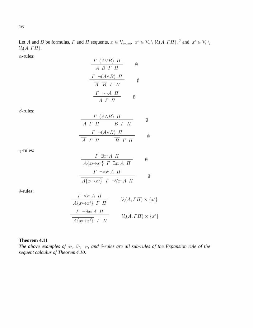
While Hypothesizing and Instantiation steps are self-explanatory, Expansion steps are parameter-ized by a sequent∆ and a set of sequentsG such that{∆} R′-reduces toG. For tableau calculi,however, this set of sequents must actually have the form{ Λ∆ | Λ∈G } because an Expansionstep cannot remove formulas from ancestor nodes. This is because these formulas are also part ofthe goals associated with other leaves in the proof tree. Therefore, although tableau calculi maysave repetition of formulas, sequent calculi have substantial advantages: Rewriting of formulas inplace is always possible, and we can remove formulas that areredundant w.r.t. the other formulasin a sequent. But this is not our subject here. For the below examples ofα-, β-, γ-, andδ-ruleswe will use the sequent calculi presentation because it is a little more explicit. When we write
∆
Π0 . . . Πn−1
R′′
we want to denote a sub-rule of the Expansion rule which is given by G := {Π0, . . . , Πn−1}and R′ := R ∪ R′′. This means that for this rule really being a sub-rule of the Expansion rulewe have to show that{∆} R′-reduces toG. By Lemma 4.5(5) and becauseR does not matterhere, it suffices that we actually show that{∆}R′′-reduces toG. Moreover, note that in old timeswhen trees grew upwards, Gerhard Gentzen would have writtenΠ0 . . . Πn−1 above the lineand∆ below, such that passing the line meant implication. In our case, passing the line meansreduction.
16
Let A andB be formulas,Γ andΠ sequents,x ∈ Vbound, xγ ∈ Vγ \ Vγ(A, ΓΠ), 7 and xδ ∈ Vδ \Vδ(A, ΓΠ).
α-rules:Γ (A∨B) Π
A B Γ Π∅
Γ ¬(A∧B) Π
A B Γ Π∅
Γ ¬¬A Π
A Γ Π∅
β-rules:Γ (A∧B) Π
A Γ Π B Γ Π∅
Γ ¬(A∨B) Π
A Γ Π B Γ Π∅
γ-rules:Γ ∃x:A Π
A{x7→xγ} Γ ∃x:A Π∅
Γ ¬∀x:A Π
A{x7→xγ} Γ ¬∀x:A Π∅
δ-rules:Γ ∀x:A Π
A{x7→xδ} Γ ΠVγ(A, ΓΠ)× {xδ}
Γ ¬∃x:A Π
A{x7→xδ} Γ ΠVγ(A, ΓΠ)× {xδ}
Theorem 4.11The above examples ofα-, β-, γ-, and δ-rules are all sub-rules of the Expansion rule of thesequent calculus of Theorem 4.10.
17
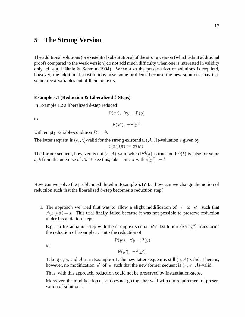
5 The Strong Version
The additional solutions (or existential substitutions) of the strong version (which admit additionalproofs compared to the weak version) do not add much difficulty when one is interested in validityonly, cf. e.g. Hahnle & Schmitt (1994). When also the preservation of solutions is required,however, the additional substitutions pose some problems because the new solutions may tearsome freeδ-variables out of their contexts:
Example 5.1 (Reduction & Liberalizedδ-Steps)
In Example 1.2 a liberalizedδ-step reduced
P(xγ), ∀y. ¬P(y)to
P(xγ), ¬P(yδ)
with empty variable-conditionR := ∅.
The latter sequent is(e,A)-valid for the strong existential(A, R)-valuatione given bye(xγ)(π) := π(yδ).
The former sequent, however, is not(e,A)-valid whenPA(a) is true andPA(b) is false for somea, b from the universe ofA. To see this, take someπ with π(yδ) := b.
How can we solve the problem exhibited in Example 5.1? I.e. how can we change the notion ofreduction such that the liberalizedδ-step becomes a reduction step?
1. The approach we tried first was to allow a slight modification of e to e′ such thate′(xγ)(π) = a. This trial finally failed because it was not possible to preserve reductionunder Instantiation-steps.
E.g., an Instantiation-step with the strong existentialR-substitution{xγ 7→yδ} transformsthe reduction of Example 5.1 into the reduction of
P(yδ), ∀y. ¬P(y)to
P(yδ), ¬P(yδ).
Takingπ, e, andA as in Example 5.1, the new latter sequent is still(e,A)-valid. There is,however, no modificatione′ of e such that the new former sequent is(π, e′,A)-valid.
Thus, with this approach, reduction could not be preserved by Instantiation-steps.
Moreover, the modification ofe does not go together well with our requirement of preser-vation of solutions.
18
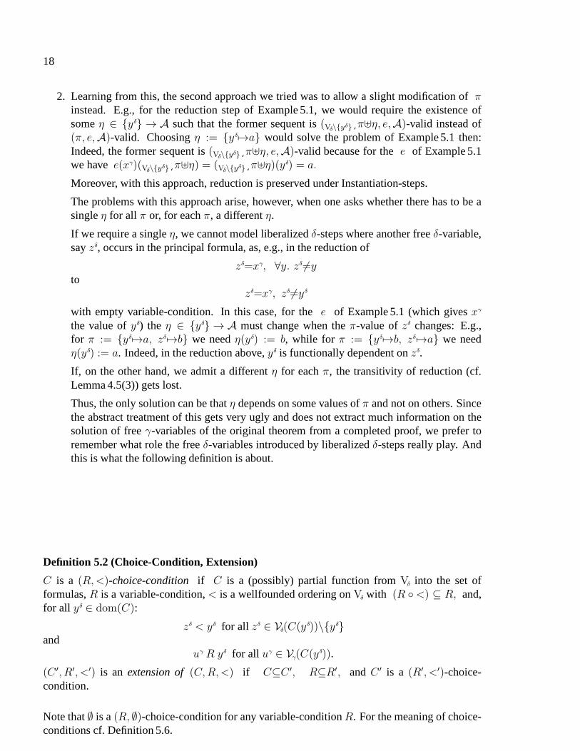
2. Learning from this, the second approach we tried was to allow a slight modification ofπinstead. E.g., for the reduction step of Example 5.1, we would require the existence ofsomeη ∈ {yδ} → A such that the former sequent is(Vδ\{yδ}¸π⊎η, e,A)-valid instead of(π, e,A)-valid. Choosingη := {yδ7→a} would solve the problem of Example 5.1 then:Indeed, the former sequent is(Vδ\{yδ}¸π⊎η, e,A)-valid because for thee of Example 5.1we havee(xγ)(Vδ\{yδ}¸π⊎η) = (Vδ\{yδ}¸π⊎η)(y
δ) = a.
Moreover, with this approach, reduction is preserved underInstantiation-steps.
The problems with this approach arise, however, when one asks whether there has to be asingleη for all π or, for eachπ, a differentη.
If we require a singleη, we cannot model liberalizedδ-steps where another freeδ-variable,sayzδ, occurs in the principal formula, as, e.g., in the reductionof
zδ=xγ, ∀y. zδ6=yto
zδ=xγ, zδ6=yδ
with empty variable-condition. In this case, for thee of Example 5.1 (which givesxγ
the value ofyδ) the η ∈ {yδ} → A must change when theπ-value ofzδ changes: E.g.,for π := {yδ7→a, zδ7→b} we needη(yδ) := b, while for π := {yδ7→b, zδ7→a} we needη(yδ) := a. Indeed, in the reduction above,yδ is functionally dependent onzδ.
If, on the other hand, we admit a differentη for eachπ, the transitivity of reduction (cf.Lemma 4.5(3)) gets lost.
Thus, the only solution can be thatη depends on some values ofπ and not on others. Sincethe abstract treatment of this gets very ugly and does not extract much information on thesolution of freeγ-variables of the original theorem from a completed proof, we prefer toremember what role the freeδ-variables introduced by liberalizedδ-steps really play. Andthis is what the following definition is about.
Definition 5.2 (Choice-Condition, Extension)
C is a (R,<)-choice-condition if C is a (possibly) partial function fromVδ into the set offormulas,R is a variable-condition,< is a wellfounded ordering onVδ with (R ◦<) ⊆ R, and,for all yδ ∈ dom(C):
zδ < yδ for all zδ ∈ Vδ(C(yδ))\{yδ}and
uγ R yδ for all uγ ∈ Vγ(C(yδ)).
(C ′, R′, <′) is an extension of(C,R,<) if C⊆C ′, R⊆R′, andC ′ is a (R′, <′)-choice-condition.
Note that∅ is a(R, ∅)-choice-condition for any variable-conditionR. For the meaning of choice-conditions cf. Definition 5.6.
19
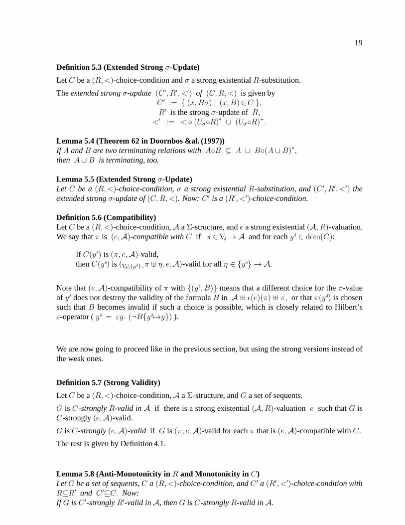
Definition 5.3 (Extended Strongσ-Update)
LetC be a(R,<)-choice-condition andσ a strong existentialR-substitution.
Theextended strongσ-update (C ′, R′, <′) of (C,R,<) is given byC ′ := { (x,Bσ) | (x,B)∈C },R′ is the strongσ-update ofR,
<′ := < ◦ (Uσ◦R)∗ ∪ (Uσ◦R)+.
Lemma 5.4 (Theorem 62 in Doornbos &al. (1997))If A andB are two terminating relations withA◦B ⊆ A ∪ B◦(A ∪ B)∗,then A ∪ B is terminating, too.
Lemma 5.5 (Extended Strongσ-Update)Let C be a (R,<)-choice-condition,σ a strong existentialR-substitution, and(C ′, R′, <′) theextended strongσ-update of(C,R,<). Now:C ′ is a (R′, <′)-choice-condition.
Definition 5.6 (Compatibility)LetC be a(R,<)-choice-condition,A aΣ-structure, ande a strong existential(A, R)-valuation.We say thatπ is (e,A)-compatible withC if π ∈Vδ → A and for eachyδ ∈ dom(C):
If C(yδ) is (π, e,A)-valid,thenC(yδ) is (Vδ\{yδ}¸π ⊎ η, e,A)-valid for all η ∈ {yδ} → A.
Note that(e,A)-compatibility ofπ with {(yδ, B)} means that a different choice for theπ-valueof yδ does not destroy the validity of the formulaB in A ⊎ ǫ(e)(π) ⊎ π, or thatπ(yδ) is chosensuch thatB becomes invalid if such a choice is possible, which is closely related to Hilbert’sε-operator (yδ = εy. (¬B{yδ7→y}) ).
We are now going to proceed like in the previous section, but using the strong versions instead ofthe weak ones.
Definition 5.7 (Strong Validity)
LetC be a(R,<)-choice-condition,A aΣ-structure, andG a set of sequents.
G is C-stronglyR-valid in A if there is a strong existential(A, R)-valuation e such thatG isC-strongly(e,A)-valid.
G isC-strongly(e,A)-valid if G is (π, e,A)-valid for eachπ that is(e,A)-compatible withC.
The rest is given by Definition 4.1.
Lemma 5.8 (Anti-Monotonicity in R and Monotonicity in C)LetG be a set of sequents,C a (R,<)-choice-condition, andC ′ a (R′, <′)-choice-condition withR⊆R′ and C ′⊆C. Now:If G is C ′-stronglyR′-valid inA, thenG isC-stronglyR-valid inA.
20
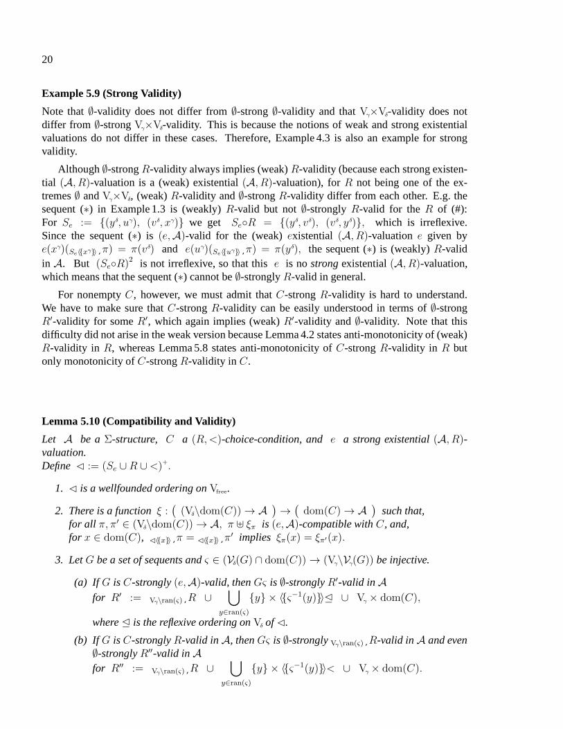
Example 5.9 (Strong Validity)
Note that∅-validity does not differ from∅-strong∅-validity and thatVγ×Vδ-validity does notdiffer from ∅-strongVγ×Vδ-validity. This is because the notions of weak and strong existentialvaluations do not differ in these cases. Therefore, Example4.3 is also an example for strongvalidity.
Although∅-strongR-validity always implies (weak)R-validity (because each strong existen-tial (A, R)-valuation is a (weak) existential(A, R)-valuation), forR not being one of the ex-tremes∅ andVγ×Vδ, (weak)R-validity and∅-strongR-validity differ from each other. E.g. thesequent (∗) in Example 1.3 is (weakly)R-valid but not∅-stronglyR-valid for theR of (#):For Se := {(yδ, uγ), (vδ, xγ)} we get Se◦R = {(yδ, vδ), (vδ, yδ)}, which is irreflexive.Since the sequent (∗) is (e,A)-valid for the (weak)existential (A, R)-valuation e given bye(xγ)(Se〈{xγ}〉¸π) = π(vδ) and e(uγ)(Se〈{uγ}〉¸π) = π(yδ), the sequent (∗) is (weakly)R-validin A. But (Se◦R)2 is not irreflexive, so that thise is nostrongexistential(A, R)-valuation,which means that the sequent (∗) cannot be∅-stronglyR-valid in general.
For nonemptyC, however, we must admit thatC-strongR-validity is hard to understand.We have to make sure thatC-strongR-validity can be easily understood in terms of∅-strongR′-validity for someR′, which again implies (weak)R′-validity and∅-validity. Note that thisdifficulty did not arise in the weak version because Lemma 4.2states anti-monotonicity of (weak)R-validity in R, whereas Lemma 5.8 states anti-monotonicity ofC-strongR-validity in R butonly monotonicity ofC-strongR-validity in C.
Lemma 5.10 (Compatibility and Validity)
Let A be aΣ-structure, C a (R,<)-choice-condition, ande a strong existential(A, R)-valuation.Define⊳ := (Se ∪R ∪<)+.
1. ⊳ is a wellfounded ordering onVfree.
2. There is a functionξ :(
(Vδ\dom(C)) → A)
→(
dom(C) → A)
such that,for all π, π′ ∈ (Vδ\dom(C)) → A, π ⊎ ξπ is (e,A)-compatible withC, and,for x ∈ dom(C), ⊳〈{x}〉¸π = ⊳〈{x}〉¸π
′ implies ξπ(x) = ξπ′(x).
3. LetG be a set of sequents andς ∈ (Vδ(G) ∩ dom(C)) → (Vγ\Vγ(G)) be injective.
(a) If G isC-strongly(e,A)-valid, thenGς is ∅-stronglyR′-valid inA
for R′ := Vγ\ran(ς)¸R ∪⋃
y∈ran(ς)
{y} × 〈{ς−1(y)}〉E ∪ Vγ × dom(C),
whereE is the reflexive ordering onVδ of⊳.
(b) If G isC-stronglyR-valid inA, thenGς is ∅-stronglyVγ\ran(ς)¸R-valid inA and even∅-stronglyR′′-valid in A
for R′′ := Vγ\ran(ς)¸R ∪⋃
y∈ran(ς)
{y} × 〈{ς−1(y)}〉< ∪ Vγ × dom(C).
21
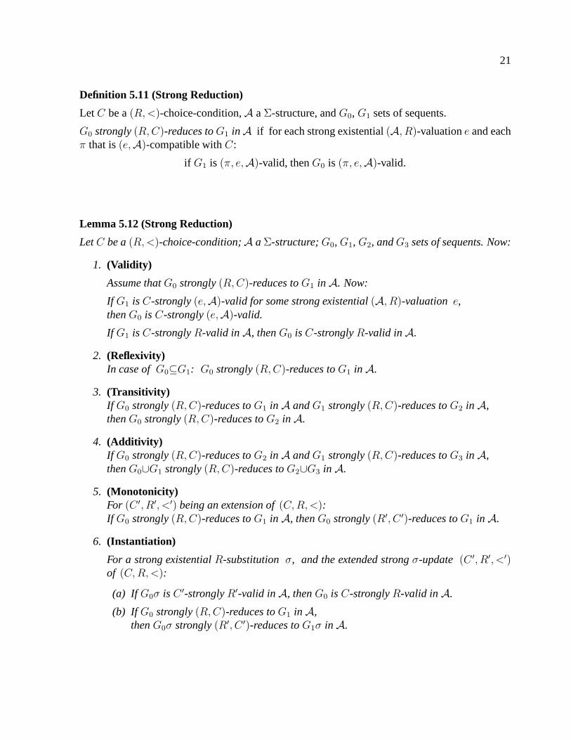
Definition 5.11 (Strong Reduction)
LetC be a(R,<)-choice-condition,A aΣ-structure, andG0, G1 sets of sequents.
G0 strongly(R,C)-reduces toG1 in A if for each strong existential(A, R)-valuatione and eachπ that is(e,A)-compatible withC:
if G1 is (π, e,A)-valid, thenG0 is (π, e,A)-valid.
Lemma 5.12 (Strong Reduction)
LetC be a(R,<)-choice-condition;A aΣ-structure;G0, G1, G2, andG3 sets of sequents. Now:
1. (Validity)
Assume thatG0 strongly(R,C)-reduces toG1 in A. Now:
If G1 isC-strongly(e,A)-valid for some strong existential(A, R)-valuation e,thenG0 is C-strongly(e,A)-valid.
If G1 isC-stronglyR-valid in A, thenG0 isC-stronglyR-valid inA.
2. (Reflexivity)In case ofG0⊆G1: G0 strongly(R,C)-reduces toG1 in A.
3. (Transitivity)If G0 strongly(R,C)-reduces toG1 in A andG1 strongly(R,C)-reduces toG2 in A,thenG0 strongly(R,C)-reduces toG2 in A.
4. (Additivity)If G0 strongly(R,C)-reduces toG2 in A andG1 strongly(R,C)-reduces toG3 in A,thenG0∪G1 strongly(R,C)-reduces toG2∪G3 in A.
5. (Monotonicity)For (C ′, R′, <′) being an extension of(C,R,<):If G0 strongly(R,C)-reduces toG1 in A, thenG0 strongly(R′, C ′)-reduces toG1 in A.
6. (Instantiation)
For a strong existentialR-substitutionσ, and the extended strongσ-update (C ′, R′, <′)of (C,R,<):
(a) If G0σ is C ′-stronglyR′-valid inA, thenG0 is C-stronglyR-valid in A.
(b) If G0 strongly(R,C)-reduces toG1 in A,thenG0σ strongly(R′, C ′)-reduces toG1σ in A.
22
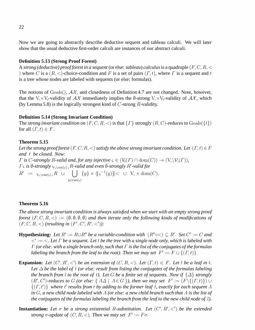
Now we are going to abstractly describe deductive sequent and tableau calculi. We will latershow that the usual deductive first-order calculi are instances of our abstract calculi.
Definition 5.13 (Strong Proof Forest)A strong (deductive) proof forest in a sequent(or else:tableau) calculusis a quadruple(F,C,R,<) whereC is a(R,<)-choice-condition andF is a set of pairs(Γ, t), whereΓ is a sequent andtis a tree whose nodes are labeled with sequents (or else: formulas).
The notions ofGoals(), AX , and closedness of Definition 4.7 are not changed. Note, however,that theVγ×Vδ-validity of AX immediately implies the∅-strongVγ×Vδ-validity of AX , which(by Lemma 5.8) is the logically strongest kind ofC-strongR-validity.
Definition 5.14 (Strong Invariant Condition)Thestrong invariant condition on(F,C,R,<) is that{Γ} strongly(R,C)-reduces toGoals({t})for all (Γ, t) ∈ F .
Theorem 5.15Let the strong proof forest(F,C,R,<) satisfy the above strong invariant condition. Let(Γ, t)∈Fand t be closed. Now:Γ isC-stronglyR-valid and, for any injectiveς ∈ (Vδ(Γ ) ∩ dom(C)) → (Vγ\Vγ(Γ )),Γς is ∅-stronglyVγ\ran(ς)¸R-valid and even∅-stronglyR′-valid for
R′ := Vγ\ran(ς)¸R ∪⋃
y∈ran(ς)
{y} × 〈{ς−1(y)}〉< ∪ Vγ × dom(C).
Theorem 5.16
The above strong invariant condition is always satisfied when we start with an empty strong proofforest (F,C,R,<) := (∅, ∅, ∅, ∅) and then iterate only the following kinds of modifications of(F,C,R,<) (resulting in(F ′, C ′, R′, <′)):
Hypothesizing: LetR′ := R∪R′′ be a variable-condition with(R′′◦<) ⊆ R′. SetC ′ := C and<′ := <. LetΓ be a sequent. Lett be the tree with a single node only, which is labeled withΓ (or else: with a single branch only, such thatΓ is the list of the conjugates of the formulaslabeling the branch from the leaf to the root). Then we may setF ′ := F ∪ {(Γ, t)}.
Expansion: Let (C ′, R′, <′) be an extension of(C,R,<). Let (Γ, t) ∈ F . Let l be a leaf int.Let∆ be the label ofl (or else: result from listing the conjugates of the formulaslabelingthe branch froml to the root oft). LetG be a finite set of sequents. Now if{∆} strongly(R′, C ′)-reduces toG (or else:{ Λ∆ | Λ∈G }), then we may setF ′ := (F\{(Γ, t)}) ∪{(Γ, t′)} wheret′ results fromt by adding to the former leafl, exactly for each sequentΛin G, a new child node labeled withΛ (or else: a new child branch such thatΛ is the list ofthe conjugates of the formulas labeling the branch from the leaf to the new child node ofl).
Instantiation: Let σ be a strong existentialR-substitution. Let(C ′, R′, <′) be the extendedstrongσ-update of(C,R,<). Then we may setF ′ := Fσ.
23
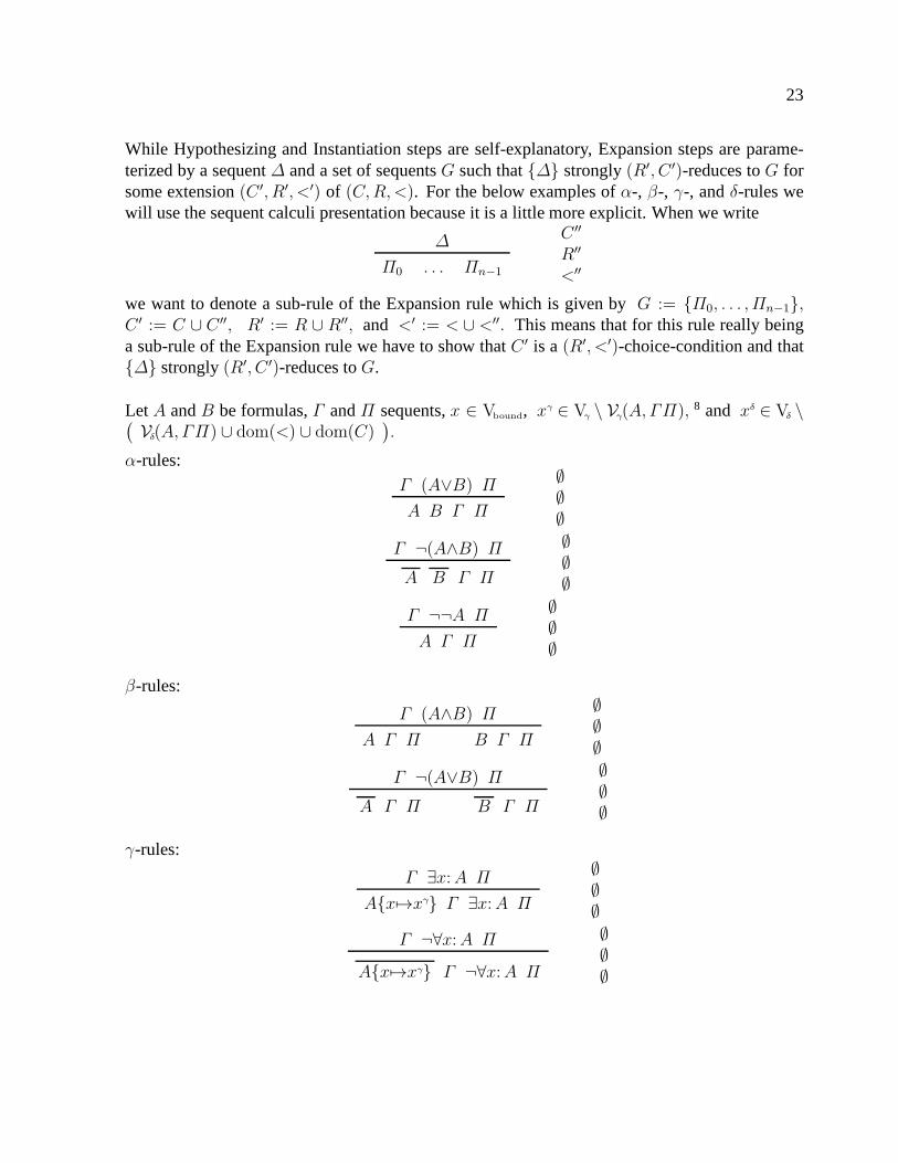
While Hypothesizing and Instantiation steps are self-explanatory, Expansion steps are parame-terized by a sequent∆ and a set of sequentsG such that{∆} strongly(R′, C ′)-reduces toG forsome extension(C ′, R′, <′) of (C,R,<). For the below examples ofα-, β-, γ-, andδ-rules wewill use the sequent calculi presentation because it is a little more explicit. When we write
∆
Π0 . . . Πn−1
C ′′
R′′
<′′
we want to denote a sub-rule of the Expansion rule which is given by G := {Π0, . . . , Πn−1},C ′ := C ∪ C ′′, R′ := R ∪ R′′, and <′ := < ∪ <′′. This means that for this rule really beinga sub-rule of the Expansion rule we have to show thatC ′ is a(R′, <′)-choice-condition and that{∆} strongly(R′, C ′)-reduces toG.
Let A andB be formulas,Γ andΠ sequents,x ∈ Vbound, xγ ∈ Vγ \ Vγ(A, ΓΠ), 8 and xδ ∈ Vδ \(
Vδ(A, ΓΠ) ∪ dom(<) ∪ dom(C))
.
α-rules:
Γ (A∨B) Π
A B Γ Π
∅∅∅
Γ ¬(A∧B) Π
A B Γ Π
∅∅∅
Γ ¬¬A Π
A Γ Π
∅∅∅
β-rules:
Γ (A∧B) Π
A Γ Π B Γ Π
∅∅∅
Γ ¬(A∨B) Π
A Γ Π B Γ Π
∅∅∅
γ-rules:
Γ ∃x:A Π
A{x7→xγ} Γ ∃x:A Π
∅∅∅
Γ ¬∀x:A Π
A{x7→xγ} Γ ¬∀x:A Π
∅∅∅
24
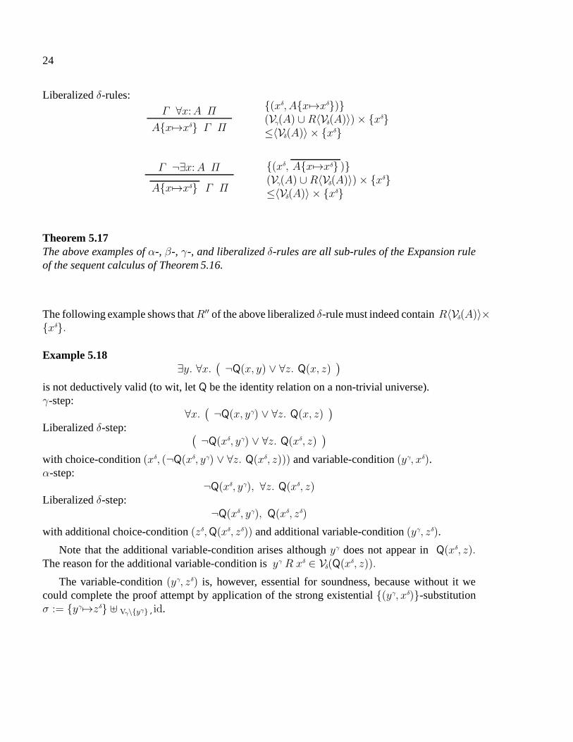
Liberalizedδ-rules:
Γ ∀x:A Π
A{x7→xδ} Γ Π
{(xδ, A{x7→xδ})}(Vγ(A) ∪ R〈Vδ(A)〉)× {xδ}≤〈Vδ(A)〉 × {xδ}
Γ ¬∃x:A Π
A{x7→xδ} Γ Π
{(xδ, A{x7→xδ} )}(Vγ(A) ∪ R〈Vδ(A)〉)× {xδ}≤〈Vδ(A)〉 × {xδ}
Theorem 5.17The above examples ofα-, β-, γ-, and liberalizedδ-rules are all sub-rules of the Expansion ruleof the sequent calculus of Theorem 5.16.
The following example shows thatR′′ of the above liberalizedδ-rule must indeed containR〈Vδ(A)〉×{xδ}.
Example 5.18∃y. ∀x.
(
¬Q(x, y) ∨ ∀z. Q(x, z))
is not deductively valid (to wit, letQ be the identity relation on a non-trivial universe).γ-step:
∀x.(
¬Q(x, yγ) ∨ ∀z. Q(x, z))
Liberalizedδ-step:(
¬Q(xδ, yγ) ∨ ∀z. Q(xδ, z))
with choice-condition(xδ, (¬Q(xδ, yγ) ∨ ∀z. Q(xδ, z))) and variable-condition(yγ, xδ).α-step:
¬Q(xδ, yγ), ∀z. Q(xδ, z)Liberalizedδ-step:
¬Q(xδ, yγ), Q(xδ, zδ)
with additional choice-condition(zδ,Q(xδ, zδ)) and additional variable-condition(yγ, zδ).
Note that the additional variable-condition arises although yγ does not appear inQ(xδ, z).The reason for the additional variable-condition isyγ R xδ ∈ Vδ(Q(x
δ, z)).
The variable-condition(yγ, zδ) is, however, essential for soundness, because without it wecould complete the proof attempt by application of the strong existential{(yγ, xδ)}-substitutionσ := {yγ7→zδ} ⊎ Vγ\{yγ}¸id.
25
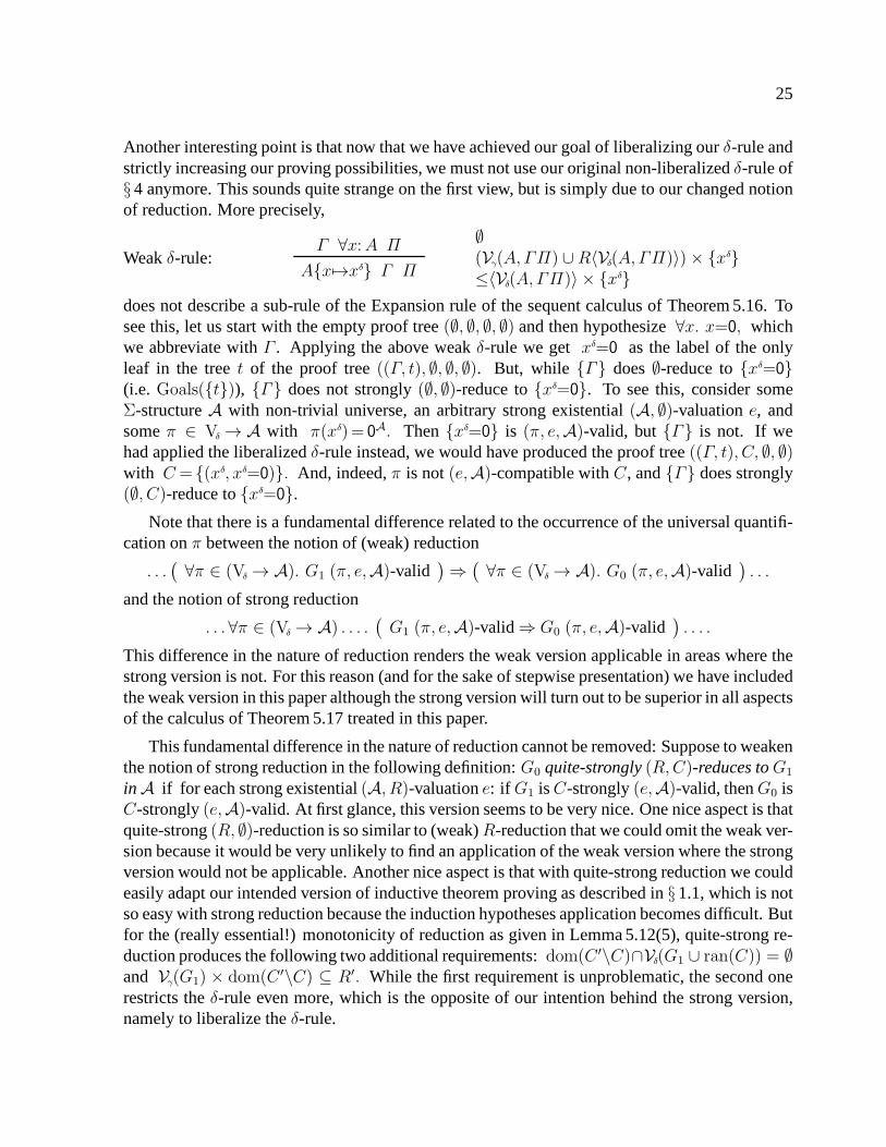
Another interesting point is that now that we have achieved our goal of liberalizing ourδ-rule andstrictly increasing our proving possibilities, we must notuse our original non-liberalizedδ-rule of§ 4 anymore. This sounds quite strange on the first view, but is simply due to our changed notionof reduction. More precisely,
Weakδ-rule:Γ ∀x:A Π
A{x7→xδ} Γ Π
∅(Vγ(A, ΓΠ) ∪ R〈Vδ(A, ΓΠ)〉)× {xδ}≤〈Vδ(A, ΓΠ)〉 × {xδ}
does not describe a sub-rule of the Expansion rule of the sequent calculus of Theorem 5.16. Tosee this, let us start with the empty proof tree(∅, ∅, ∅, ∅) and then hypothesize∀x. x=0, whichwe abbreviate withΓ . Applying the above weakδ-rule we get xδ=0 as the label of the onlyleaf in the treet of the proof tree((Γ, t), ∅, ∅, ∅). But, while {Γ} does∅-reduce to{xδ=0}(i.e. Goals({t})), {Γ} does not strongly(∅, ∅)-reduce to{xδ=0}. To see this, consider someΣ-structureA with non-trivial universe, an arbitrary strong existential (A, ∅)-valuatione, andsomeπ ∈ Vδ → A with π(xδ)= 0A. Then{xδ=0} is (π, e,A)-valid, but {Γ} is not. If wehad applied the liberalizedδ-rule instead, we would have produced the proof tree((Γ, t), C, ∅, ∅)with C = {(xδ, xδ=0)}. And, indeed,π is not(e,A)-compatible withC, and{Γ} does strongly(∅, C)-reduce to{xδ=0}.
Note that there is a fundamental difference related to the occurrence of the universal quantifi-cation onπ between the notion of (weak) reduction
. . .(
∀π ∈ (Vδ → A). G1 (π, e,A)-valid)
⇒(
∀π ∈ (Vδ → A). G0 (π, e,A)-valid)
. . .
and the notion of strong reduction
. . .∀π ∈ (Vδ → A) . . . .(
G1 (π, e,A)-valid⇒ G0 (π, e,A)-valid)
. . . .
This difference in the nature of reduction renders the weak version applicable in areas where thestrong version is not. For this reason (and for the sake of stepwise presentation) we have includedthe weak version in this paper although the strong version will turn out to be superior in all aspectsof the calculus of Theorem 5.17 treated in this paper.
This fundamental difference in the nature of reduction cannot be removed: Suppose to weakenthe notion of strong reduction in the following definition:G0 quite-strongly(R,C)-reduces toG1
in A if for each strong existential(A, R)-valuatione: if G1 isC-strongly(e,A)-valid, thenG0 isC-strongly(e,A)-valid. At first glance, this version seems to be very nice. One nice aspect is thatquite-strong(R, ∅)-reduction is so similar to (weak)R-reduction that we could omit the weak ver-sion because it would be very unlikely to find an application of the weak version where the strongversion would not be applicable. Another nice aspect is thatwith quite-strong reduction we couldeasily adapt our intended version of inductive theorem proving as described in§ 1.1, which is notso easy with strong reduction because the induction hypotheses application becomes difficult. Butfor the (really essential!) monotonicity of reduction as given in Lemma 5.12(5), quite-strong re-duction produces the following two additional requirements: dom(C ′\C)∩Vδ(G1 ∪ ran(C)) = ∅and Vγ(G1) × dom(C ′\C) ⊆ R′. While the first requirement is unproblematic, the second onerestricts theδ-rule even more, which is the opposite of our intention behind the strong version,namely to liberalize theδ-rule.
26
Moreover, note that (as far as Theorem 5.17 is concerned) thechoice-conditions do not have anyinfluence on our proofs and may be discarded. We could, however, use them for the followingpurposes:
1. We could use the choice-conditions in order to weaken our requirements for our set ofaxiomsAX : Instead of∅-strongVγ×Vδ-validity of AX the weakerC-strongVγ×Vδ-validityof AX is sufficient for Theorem 5.15.
2. If we add a functional behavior to a choice-conditionC, i.e. if we require that for(xδ, A) ∈C the value forxδ is not just an arbitrary one from the set of values that makeA invalid,but a unique element of this set given by some choice-function, then we can use the choice-conditions for simulating the behavior of theδ+
+
-rule of Beckert &al. (1993) by using thesame freeδ-variable for the sameC-value and by later equating freeδ-variables whoseC-values become equal during the proof.
3. Moreover, the choice-conditions may be used to get more interesting answers:
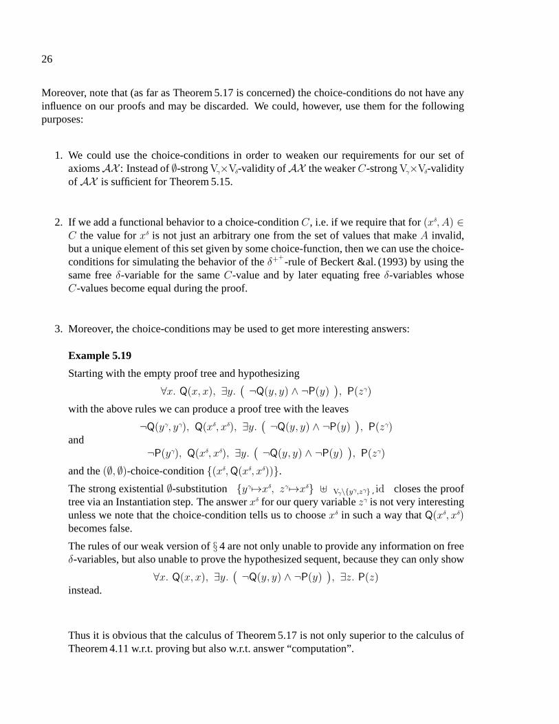
Example 5.19
Starting with the empty proof tree and hypothesizing
∀x. Q(x, x), ∃y.(
¬Q(y, y) ∧ ¬P(y))
, P(zγ)
with the above rules we can produce a proof tree with the leaves
¬Q(yγ, yγ), Q(xδ, xδ), ∃y.(
¬Q(y, y) ∧ ¬P(y))
, P(zγ)and
¬P(yγ), Q(xδ, xδ), ∃y.(
¬Q(y, y) ∧ ¬P(y))
, P(zγ)
and the(∅, ∅)-choice-condition{(xδ,Q(xδ, xδ))}.
The strong existential∅-substitution {yγ7→xδ, zγ 7→xδ} ⊎ Vγ\{yγ,zγ}¸id closes the prooftree via an Instantiation step. The answerxδ for our query variablezγ is not very interestingunless we note that the choice-condition tells us to choosexδ in such a way thatQ(xδ, xδ)becomes false.
The rules of our weak version of§ 4 are not only unable to provide any information on freeδ-variables, but also unable to prove the hypothesized sequent, because they can only show
∀x. Q(x, x), ∃y.(
¬Q(y, y) ∧ ¬P(y))
, ∃z. P(z)instead.
Thus it is obvious that the calculus of Theorem 5.17 is not only superior to the calculus ofTheorem 4.11 w.r.t. proving but also w.r.t. answer “computation”.
27
Finally, note that (concerning the calculus of Theorem 5.17) the ordering< is not needed at allwhen in the liberalizedδ-steps we always choose a completely new freeδ-variablexδ that doesnot occur elsewhere and when in the Hypothesizing steps we guarantee thatran(R′′) containsonly new freeδ-variables that have not occurred before. The former is reasonable anyhow, be-cause the freeδ-variables introduced by previous liberalizedδ-steps cannot be used because theyare indom(C) and the use of a freeδ-variable from the input hypothesis deteriorates the result ofour proof by giving this freeδ-variable an existential meaning (because it puts it intodom(C)) asexplained in Theorem 5.15. The latter does not seem to be restrictive for any reasonable applica-tion.
All in all, when interested in proving only, the (compared tothe weak version) additional choice-condition and ordering of the strong version do not produce any overhead because they can simplybe omitted. This is interesting because choice-conditionsor Hilbert’s ε-expressions are some-times considered to make proofs quite complicated. When interested in answer “computation”,however, they could turn out to be useful.
W.r.t. the calculus of Theorem 5.17 we thus may conclude thatthe strong version is generallybetter than the weak version and the only overhead seems to bethat we have to compute transitiveclosures when checking whether a substitutionσ is really a strong existentialR-substitution andwhen computing the strongσ-update ofR. But we actually do not have to compute the transitiveclosure at all, because the only essential thing is the circularity-check which can be done on abipartite9 graph generating the transitive closures. This checking isin the worst case linear in
|R| +∑
σ
(
|Uσ| + |Eσ|)
and is expected to perform at least as well as an optimally integrated version (i.e. one withoutconversion of term-representation) of the linear unification algorithm of Paterson & Wegman(1978) in the standard framework of Skolemization and unification. Note, however, that thechecking for strong existentialR-substitutions can also be implemented with any other unificationalgorithm.
Not really computing the transitive closure enables another refinement that allows us to goeven beyond the fascinatingstrong Skolemizationof Nonnengart (1996). The basic idea of Nonnengart(1996) can be translated into our framework in the followingsimplified way.
Instead of proving∀x: (A∨B) it may be advantageous to prove the stronger∀x:A ∨ ∀x:B,because after applications ofα- and liberalizedδ-rules to ∀x:A ∨ ∀x:B, resulting inA{x7→xδ
A}, B{x7→xδ
B}, the variable-conditions introduced forxδ
A andxδ
B may be smaller thanthe variable-condition introduced foryδ after applying these rules to∀x: (A∨B), resulting inA{x7→yδ}, B{x7→yδ}, i.e.R〈{xδ
A}〉 andR〈{xδ
B}〉 may beproper subsets ofR〈{yδ}〉. Thereforethe proof of ∀x:A ∨ ∀x:B may be simpler than the proof of∀x: (A∨B). The nice aspect ofNonnengart (1996) is that the proofs of∀x:A and ∀x: (A∨B) can be done in parallel with-out extra costs, such that the bigger variable-condition becomes active only if we decide that thesmaller variable-condition is not enough to prove∀x:A and we had better prove the weaker∀x: (A∨B).
28
The disadvantage of the strong Skolemization approach of Nonnengart (1996), however,is that we have to decide whether to prove either∀x:A or else ∀x:B in parallel to∀x: (A∨B). In terms of Hilbert’sε-operator, this asymmetry can be understood from the ar-gumentation of Nonnengart (1996), which, for some new variable z ∈ Vbound and t denotingthe term εz: (¬A{x7→z} ∧ (A ∨ x=z)), employs the logical equivalence of∀x: (A∨B) with∀x:A ∨ ∀x: (B{x7→t}) and then the logical equivalence of∀x:A with ∃x: (A{x7→t}).
Now, if we do not really compute the transitive closures in our strong version, wecan prove A{x7→xδ
A}, B{x7→xδ
B} in parallel and may later decide to prove the strongerA{x7→yδ}, B{x7→yδ} instead, simply by merging the nodes forxδ
A andxδ
B and substitutingxδ
A andxδ
B with yδ.
6 Conclusion
All in all, we have presented an easy to read combination of raising, explicit variable dependencyrepresentation, the liberalizedδ-rule, and preservation of solutions for first-order deductive the-orem proving. Our motivation was not only to make these subjects more popular, but also toprovide the foundation for our work on inductive theorem proving (cf. Wirth (1999)) where thepreservation of solutions is indispensable.
To our knowledge10 we have presented on the one hand the first sound combination of ex-plicit variable dependency representation and the liberalizedδ-rule and on the other hand the firstframework for preservation of solutions in full first-orderlogic.
Finally, the described problems with the development of thestrong version reveal unexpecteddetails on the nature of the liberalizedδ-rule, and the discussion at the end of§ 5 opens up severalnew research directions.
29
7 The Proofs
Proof of Lemma 3.6
(1): Since e′ is a [strong] existential(A, R′)-valuation,Se′◦R′ [ ◦ (Se′◦R
′)∗] is irreflexive [anda wellfounded ordering]. SinceR⊆R′, we haveSe′◦R [ ◦ (Se′◦R)∗] ⊆ Se′◦R
′ [ ◦ (Se′◦R′)∗].
Thus Se′◦R [ ◦ (Se′◦R)∗] is irreflexive [and a wellfounded ordering], too. Therefore, settinge := e′, we get a [strong] existential(A, R)-valuation trivially satisfying the requirements.
(2): Here we denote concatenation (product) of relations ‘◦’ simply by juxtaposition and assumeit to have higher priority than any other binary operator. Let e′ be some [strong] existential(A, R′)-valuation. DefineSe := Se′Eσ ∪ Uσ and the [strong] existential(A, R)-valuation e by(x∈Vγ, π′ ∈Se〈{x}〉 → A):
e(x)(π′) := eval(A⊎ ǫ(e′)(π) ⊎ π)(σ(x))
whereπ ∈ Vδ → A is an arbitrary extension ofπ′. For this definition to be okay, we have to provethe following claims:Claim 1:Fory ∈ Vδ(σ(x)), the choice ofπ ⊇ π′ does not influence the value ofπ(y).Claim 2:Forx′ ∈ Vγ(σ(x)), the choice ofπ ⊇ π′ does not influence the value ofǫ(e′)(π)(x′).Claim 3:For the weak version we have to show thatSeR is irreflexive.Claim 4:For the strong version we have to show that(SeR)+ is a wellfounded ordering.Proof of Claim 1:y ∈Vδ(σ(x)) means(y, x)∈Uσ. By definition ofSe we have(y, x)∈Se, i.e.y ∈ Se〈{x}〉 = dom(π′). Q.e.d. (Claim 1)Proof of Claim 2: x′ ∈Vγ(σ(x)) means (x′, x)∈Eσ. Thus by definition ofSe we haveSe′{(x
′, x)} ⊆ Se, i.e. Se′〈{x′}〉 ⊆ Se〈{x}〉 = dom(π′). Therefore ǫ(e′)(π)(x′) =
e′(x′)(Se′〈{x′}〉¸π) = e′(x′)(Se′ 〈{x
′}〉¸π′). Q.e.d. (Claim 2)
Proof of Claim 3:Since SeR = Se′EσR ∪ UσR andUσR is irreflexive (asσ is an existentialR-substitution), it suffices to show irreflexivity ofSe′EσR. SinceR′ is theσ-update ofR, this isequal toSe′R
′, which is irreflexive becausee′ is an existential(A, R′)-valuation.Q.e.d. (Claim 3)
Proof of Claim 4:Sinceσ is a strong existentialR-substitution,(UσR)+ is a wellfounded or-dering. Thus, if (SeR)+ = (Se′EσR ∪ UσR)+ = (UσR)+ ∪ (UσR)∗(Se′EσR(UσR)∗)
+
is not a wellfounded ordering, there must be an infinite descending sequence of theform y2i+2 (UσR)∗ y2i+1 (Se′EσR(UσR)∗)
+
y2i for all i ∈ N. But theny2i+3 (Se′EσR(UσR)∗)
+
y2i+2 (UσR)∗ y2i+1, which contradicts the wellfoundedness of(Se′EσR(UσR)∗)
+
(UσR)∗ = (Se′EσR(UσR)∗)+
= (Se′R′)+, where the latter step is due toR′
being the strongσ-update ofR. The latter relation is a wellfounded ordering, however, becausee′ is a strong existential(A, R′)-valuation. Q.e.d. (Claim 4)
Now, for π ∈ Vδ → A and x ∈ Vγ we haveǫ(e)(π)(x) = e(x)(Se〈{x}〉¸π) = eval(A ⊎ ǫ(e′)(π) ⊎ π)(σ(x))
i.e. ǫ(e)(π) = σ ◦ eval(A⊎ ǫ(e′)(π) ⊎ π). Q.e.d. (Lemma 3.6)
Proof of Lemma 4.2This a trivial consequence of Lemma 3.6(1). Q.e.d. (Lemma 4.2)
30
Proof of Lemma 4.5 (1), (2), (3), and (4) are trivial. Note that (5) is a trivial consequence ofLemma 3.6(1).
(6a):Suppose thatG0σ is R′-valid in A. Then there is some existential(A, R′)-valuatione′ suchthatG0σ is (e′,A)-valid. Then, by Lemma 3.6(2), there is some existential(A, R)-valuationesuch that for allπ ∈ Vδ → A: ǫ(e)(π) = σ ◦ eval(A ⊎ ǫ(e′)(π) ⊎ π). Moreover, fory ∈ Vδ wehave: π(y) = eval(A ⊎ ǫ(e′)(π) ⊎ π)(y),i.e. ǫ(e)(π) ⊎ π = (σ ⊎ Vδ
¸id) ◦ eval(A⊎ ǫ(e′)(π) ⊎ π).Thus, for any formulaB, we have
eval(A ⊎ ǫ(e)(π) ⊎ π)(B) =eval(A ⊎ ((σ ⊎ Vδ
¸id) ◦ eval(A ⊎ ǫ(e′)(π) ⊎ π)))(B) =eval(A ⊎ ǫ(e′)(π) ⊎ π)(Bσ),
the latter step being due to the Substitution-Lemma.
Thus, for any set of sequentsG′:
(e,A)-validity of G′ is logically equivalent to(e′,A)-validity of G′σ . (:§)
Especially,G0 is (e,A)-valid. Thus,G0 is R-valid inA.
(6b): Let e′ be some existential(A, R′)-valuation and suppose thatG1σ is (e′,A)-valid. Lete bethe existential(A, R)-valuation given by Lemma 3.6(2). Then, by (§) in the proof of (6a),G1 is(e,A)-valid. By assumption,G0 R-reduces toG1. Thus,G0 is (e,A)-valid. By (§) in the proofof (6a), this means thatG0σ is (e′,A)-valid. Q.e.d. (Lemma 4.5)
Proof of Theorem 4.9SinceAX isVγ×Vδ-valid, t is closed, andR ⊆ Vγ×Vδ, by Lemma 4.5(5),Goals({t}) isR-valid.Since (Γ, t)∈F and(F,R) satisfies the invariant condition,{Γ} R-reduces toGoals({t}). Allin all, by Lemma 4.5(1),Γ isR-valid. Q.e.d. (Theorem 4.9)
Proof of Theorem 4.10(∅, ∅) trivially satisfies the invariant condition. For the iteration steps, let(Γ ′′, t′′) ∈ F ′. Assumingthe invariant condition for(F,R), we have to show that{Γ ′′} R′-reduces toGoals({t′′}).
Hypothesizing:In case of (Γ ′′, t′′)∈F, {Γ ′′} R-reduces toGoals({t′′}) by assumption, andthen, due toR⊆R′ and Lemma 4.5(5),{Γ ′′} R′-reduces toGoals({t′′}). Otherwise we have(Γ ′′, t′′)= (Γ, t). Then {Γ ′′} = {Γ} = Goals({t}) = Goals({t′′}). Thus, by Lemma 4.5(2),{Γ ′′} R′-reduces toGoals({t′′}).
Expansion:In case of(Γ ′′, t′′)∈F, {Γ ′′}R-reduces toGoals({t′′}) by assumption, and then, dueto R⊆R′ and Lemma 4.5(5),{Γ ′′} R′-reduces toGoals({t′′}). Otherwise we have(Γ ′′, t′′) =(Γ, t′). Since Goals({t})\{∆} ⊆ Goals({t′}), by Lemma 4.5(2),Goals({t})\{∆} R′-reducesto Goals({t′}). Thus, since by assumption{∆} R′-reduces to a subset ofGoals({t′}), by Lem-ma 4.5(4)Goals({t}) R′-reduces toGoals({t′}). Moreover, due to (Γ, t)∈F, by assump-tion {Γ} R-reduces toGoals({t}). Thus, by R⊆R′ and Lemma 4.5(5),{Γ} R′-reduces toGoals({t}). Thus, sinceGoals({t})R′-reduces toGoals({t′}), by Lemma 4.5(3){Γ}R′-reducestoGoals({t′}), i.e.{Γ ′′} R′-reduces toGoals({t′′}).
Instantiation:There is some(Γ, t) ∈ F such that (Γ, t)σ = (Γ ′′, t′′). By assumption,{Γ}R-reduces toGoals({t}). By Lemma 4.5(6),{Γσ} R′-reduces toGoals({t})σ, i.e. {Γ ′′} R′-reduces toGoals({t′′}). Q.e.d. (Theorem 4.10)
31
Proof of Theorem 4.11
Let A be an arbitraryΣ-structure (Σ-algebra). We only prove the first example of each kind ofrule to be a sub-rule of the Expansion rule and leave the rest as an exercise.
α-rule: We have to show that{Γ (A∨B) Π} ∅-reduces to{A B Γ Π} in A. This istrivial, however, because(e,A)-validity of the two sets is logically equivalent for each existential(A, ∅)-valuatione.
β-rule:We have to show that{Γ (A∧B) Π} ∅-reduces to{A Γ Π, B Γ Π} in A. This istrivial, however, because(e,A)-validity of the two sets is logically equivalent for each existential(A, ∅)-valuatione.
γ-rule: We have to show that{Γ ∃x:A Π} ∅-reduces to{A{x7→xγ} Γ ∃x:A Π} in A.This is the case, however, because(e,A)-validity of the two sets is logically equivalent for eachexistential(A, ∅)-valuatione. The direction from left to right is given because the formersequentis a sub-sequent of the latter. The other direction, which isthe only one we actually have to showhere, is also clear because(π, e,A)-validity of A{x7→xγ} implies (π, e,A)-validity of ∃x:A.Although this is clear, we should be a little more explicit here because the standard semanticdefinition of∃ (cf. e.g. Wirth (1997), p. 188) does not use freeγ-variables and is somewhat morecomplicated than it could be in terms of freeγ-variables. Moreover, in the note above the theoremwe remarked that the restriction onxγ not occurring in the former sequent is not really necessary.Thus, in order to be more explicit here, assume that the latter sequent is(e,A)-valid for someexistential(A, ∅)-valuatione. Let π ∈ Vδ → A. We have to show that the former sequent is(π, e,A)-valid. If this is not the case,A{x7→xγ} must be(π, e,A)-valid. Let yδ ∈ Vδ\Vδ(A).Then, sinceA{x7→yδ}{yδ7→xγ} is equal to A{x7→xγ}, we know that A{x7→yδ}{yδ7→xγ} isvalid in A⊎ǫ(e)(π)⊎π. Then, by the Substitution-Lemma,A{x7→yδ} is valid in A⊎ǫ(e)(π)⊎π′
for π′ ∈ Vδ → A given by Vδ\{yδ}¸π′ := Vδ\{yδ}¸π and π′(yδ) := ǫ(e)(π)(xγ). By the standard
semantic definition of∃ and since quantification onx cannot occur inA (as∃x:A is a formula inour restricted sense, cf.§ 1.4), this means that∃x:(A{x7→yδ}{yδ7→x}) is valid inA⊎ ǫ(e)(π)⊎π.Sinceyδ does not occur inA, this formula is equal to∃x:A, which means that the former sequentis (π, e,A)-valid as was to be shown.
δ-rule: We have to show that{Γ ∀x:A Π} R′′-reduces to {A{x7→xδ} Γ Π} in A forR′′ = Vγ(A, ΓΠ)× {xδ}. Assume that the latter sequent is(e,A)-valid for some existentialR′′-valuatione. Let π ∈ Vδ → A. We have to show that the former sequent is(π, e,A)-valid.If some formula inΓΠ is (π, e,A)-valid, then the former sequent is(π, e,A)-valid, too. Oth-erwise,ΓΠ is not only invalid in A ⊎ ǫ(e)(π) ⊎ π, but also in A ⊎ ǫ(e)(π) ⊎ π′ for allπ′ ∈ Vδ → A with Vδ\{xδ}¸π
′ = Vδ\{xδ}¸π, simply becausexδ does not occur inΓΠ. Because ofVγ(ΓΠ)× {xδ} ⊆ R′′, we know thatΓΠ must be even invalid inA ⊎ ǫ(e)(π′) ⊎ π′. Since thelatter sequent is assumed to be(e,A)-valid, this means thatA{x7→xδ} is (π′, e,A)-valid. Becauseof Vγ(A{x7→xδ}) × {xδ} = Vγ(A) × {xδ} ⊆ R′′, we know thatA{x7→xδ} must be even validin A ⊎ ǫ(e)(π) ⊎ π′ for all π′ ∈ Vδ → A with Vδ\{xδ}¸π
′ = Vδ\{xδ}¸π. By the standard semanticdefinition of∀ (cf. e.g. Wirth (1997), p. 188) and since quantification onx cannot occur inA (as∀x:A is a formula in our restricted sense, cf.§1.4), this means that∀x:(A{x7→xδ}{xδ7→x}) isvalid inA⊎ǫ(e)(π)⊎π. Sincexδ does not occur inA, this formula is equal to∀x:A, which meansthat the former sequent is(π, e,A)-valid as was to be shown. Q.e.d. (Theorem 4.11)
32
Proof of Lemma 5.4
Since in Doornbos &al. (1997) Theorem 62 and especially its proof (which is used to illustratethe application of the very special framework of that paper)are not easy to read, we give aneasier proof here that requires fewer set theoretical preconditions and uses induction only onω. It proceeds by showing the existence of a refutational element in a nonempty set of infinitedescending sequences.
Set F := dom(A) ∪ ran(A) ∪ dom(B) ∪ ran(B). We show that C := { t : N → F |∀i∈N. ti (A∪B) ti+1 } is empty. Otherwise we can chooses ∈ C and families(Di)i∈N and(Ei)i∈N+
of subsets ofF inductively in the following way:D0 := { t0 | t∈C }. Chooses0 such that it isB-irreducible inD0, i.e. such thats0 ∈D0 andthere is not′ ∈ D0 such thats0 B t′.For n ∈ N+: Dn := { tn | t∈C ∧ ∀i≺ n. ti = si ∧ sn−1 A tn }. En := { tn |t∈C ∧ ∀i≺n. ti = si ∧ sn−1 B tn }. If En is nonempty we choosesn from En. Otherwise,we choosesn to beB-irreducible inDn.
Sinces ∈ C andA is terminating, there is some minimaln ∈ N with sn B sn+1. We haven≻ 0,because otherwises0 B s1 ∈ D0 contradicts the choice ofs0. Thus, sn−1 (A\B) sn B sn+1.Since sn−1 (A\B) sn, we know thatsn was chosen not fromEn, butB-irreducible inDn. Dueto A◦B ⊆ A ∪ B◦(A ∪B)∗ we get two possible cases now.
sn−1 A sn+1: Then s0 . . . sn−1sn+1sn+2 . . . is an element ofC. Thus, sn+1∈Dn. Due tosn B sn+1, this contradictssn beingB-irreducible inDn.
sn−1 (B◦(A ∪ B)∗) sn+1: Then there are somem ∈ N and somes0 . . . sn−1u0 . . . umsn+2sn+3 . . . in C with sn−1 B u0 and um= sn+1 . Thus, u0∈En, i.e.En
is not empty. But this contradicts the fact thatsn was not chosen fromEn. Q.e.d. (Lemma 5.4)
Proof of Lemma 5.5
Here we denote concatenation (product) of relations ‘◦’ simply by juxtaposition and assume it tohave higher priority than any other binary operator.
Claim 1: R′<′ ⊆ R′.Proof of Claim 1: Since C is a (R,<)-choice-condition, we have R< ⊆ R. Thus,R′<′ = EσR(UσR)∗(<(UσR)∗ ∪ (UσR)+) = Eσ(RUσ)
∗R<(UσR)∗ ∪ EσR(UσR)∗(UσR)+ ⊆Eσ(RUσ)
∗R(UσR)∗ ∪ EσR(UσR)∗(UσR)+ = EσR(UσR)∗(UσR)∗ ∪ EσR(UσR)+ =EσR(UσR)∗ = R′. Q.e.d. (Claim 1)
33
Claim 2:<′ is a wellfounded ordering onVδ.Proof of Claim 2:SinceC is a(R,<)-choice-condition, we know that< is a wellfounded order-ing onVδ and R< ⊆ R.Thus UσR< ⊆ UσR,
(UσR)+< = (UσR)∗UσR< ⊆ (UσR)∗UσR = (UσR)+,and <(UσR)∗< = << ∪ <(UσR)+< ⊆ < ∪ <(UσR)+ = <(UσR)∗.Sinceσ is a strong existentialR-substitution, we know that(UσR)+ is a is a wellfounded orderingonVδ. By Lemma 5.4 (settingA := <−1 andB := (UσR)−1) by the first of the above contain-ments, we know that<−1 ∪ (UσR)−1 is terminating, which (due to<′ = <(UσR)∗ ∪ (UσR)+ )means that>′ is terminating, too. Finally<′ is also transitive, since by the above containments:
<(UσR)∗<(UσR)∗ ⊆ <(UσR)∗(UσR)∗ = <(UσR)∗ ⊆ <′
and <(UσR)∗(UσR)+ = <(UσR)+ ⊆ <(UσR)∗ ⊆ <′
and (UσR)+<(UσR)∗ ⊆ (UσR)+(UσR)∗ = (UσR)+ ⊆ <′
and (UσR)+(UσR)+ ⊆ (UσR)+ ⊆ <′. Q.e.d. (Claim 2)
Claim 3:For allyδ ∈ dom(C ′): For allzδ ∈ Vδ(C′(yδ))\{yδ}: zδ <′ yδ.
Proof of Claim 3: Let zδ ∈ Vδ(C′(yδ))\{yδ}. By the definition of C ′ this means
zδ∈Vδ(C(yδ))\{yδ} or there is someuγ ∈ Vγ(C(yδ)) with zδ Uσ uγ. SinceC is a (R,<)-choice-condition, we havezδ < yδ or zδ Uσ u
γ R yδ. Thus, by definition of<′ we havezδ <′ yδ.Q.e.d. (Claim 3)
Claim 4:For allyδ ∈ dom(C ′): For alluγ ∈ Vγ(C′(yδ)): uγ R′ yδ.
Proof of Claim 4:Let uγ ∈ Vδ(C′(yδ)). By the definition ofC ′ there is somevγ ∈ Vγ(C(yδ)) with
uγ Eσ vγ. SinceC is a(R,<)-choice-condition, we havevγ R yδ. Thus, by definition ofR′ wehave uγ R′ yδ. Q.e.d. (Claim 4) Q.e.d. (Lemma 5.5)
Proof of Lemma 5.8SinceG is C ′-stronglyR′-valid in A, there is some strong existential(A, R′)-valuatione′ suchthatG is C ′-strongly(e′,A)-valid. Let e be the strong existential(A, R)-valuation with ǫ(e) =ǫ(e′) given by Lemma 3.6(1) due toR⊆R′. Let π be (e,A)-compatible withC. It suffices toshow thatG is (π, e,A)-valid. Since the notion of(e,A)-compatibility does not depend on theprecise form ofe besidesǫ(e), we know thatπ is also(e′,A)-compatible withC. Due to C ′⊆C,π is also(e′,A)-compatible withC ′. Finally, sinceG is C ′-strongly(e′,A)-valid, we concludethatG is (π, e′,A)-valid, i.e.(π, e,A)-valid. Q.e.d. (Lemma 5.8)
Proof of Lemma 5.10
(1): SinceC is a (R,<)-choice-condition, we know that< is a wellfounded ordering onVδ andR ⊆ Vγ×Vδ. Moreover, we haveSe ⊆ Vδ×Vγ and Vγ∩Vδ = ∅. Thus, if⊳ is not wellfounded,then there is an infinitely descending sequence of the formy2i+2 Se y2i+1 (R ◦ ≤) y2i for alli ∈ N. SinceC is a (R,<)-choice-condition, we know that(R ◦<) ⊆ R. Thus, we gety2i+2 Se y2i+1 R y2i for all i ∈ N. This means that(Se◦R)+ is not wellfounded, which contradictsthe assumption thate is a strong existential(A, R)-valuation.
34
(2): Let π ∈ (Vδ\dom(C)) → A. By noetherian induction on⊳ and with the help of a choicefunction we can define some ∈ Vfree → A in the following way: Forx ∈ Vγ: (x) :=e(x)(Se〈{x}〉¸). For x ∈ Vδ\dom(C): (x) := π(x). For x ∈ dom(C): (x) := a, wherea is an element of the universe ofA such that, if possible,C(x) is not (Vδ
¸, e,A)-valid. Forthis definition to be okay, we have to show, for eachx ∈ Vfree, that(x) is defined in terms of⊳〈{x}〉¸. In case of x∈Vγ, this is obvious becauseSe⊆⊳. In case of x∈Vδ\dom(C), thisis trivial. Thus, letx ∈ dom(C). SinceC is a (R,<)-choice-condition, we havezδ < x forall zδ ∈ Vδ(C(x))\{x} and uγ R x for all uγ ∈ Vγ(C(x)). Thus, sinceR⊆⊳, by induc-tion hypothesis,(Vδ
¸, e,A)-validity of C(x) means validity ofC(x) in A⊎. Moreover, since<⊆⊳, we know that (x) is defined in terms ofVfree(C(x))\{x}¸ ⊆ ⊳〈{x}〉¸. Finally, we defineξπ := dom(C)¸.
For showing thatπ⊎ξπ is (e,A)-compatible withC, let yδ ∈ dom(C) and suppose thatC(yδ)is (π⊎ξπ, e,A)-valid, i.e.(Vδ
¸, e,A)-valid. Thus, by definition of , we know that, for allη ∈{yδ} → A, C(yδ) is (Vδ\{yδ}¸⊎η, e,A)-valid, i.e.(π⊎Vδ\{yδ}¸ξπ⊎η, e,A)-valid. The rest is trivial.
(3a):Let ξ be given as in (2). Definee′ viae′(x)(τ) := ξπ(ς
−1(x)) (x∈ ran(ς), τ ∈ ((Vδ\dom(C)) ∩⊳〈{ς−1(x)}〉) → A, whereπ ∈(Vδ\dom(C)) → A an arbitrary extension ofτ ) ande′(x)(τ) := e(x)(Se〈{x}〉¸(π⊎ξπ)) (x∈Vγ\ran(ς), τ ∈ ((Vδ\dom(C)) ∩⊳〈{x}〉) → A, whereπ ∈ (Vδ\dom(C)) → A an arbitrary extension ofτ ).Note that this definition is okay because the choice ofπ does not matter: For the firstπ thisis directly given by (2). For the secondπ we have: Se〈{x}〉¸π ⊆ ⊳〈{x}〉¸π ⊆ τ, and, fory ∈ dom(C) ∩ Se〈{x}〉, by (2),ξπ(y) is already determined by⊳〈{y}〉¸π ⊆ ⊳〈{x}〉¸π ⊆ τ.
Then Se′ = Vδ\dom(C)¸id ◦
( ⋃
y∈ran(ς)
⊳〈{ς−1(y)}〉 × {y} ∪⋃
x∈Vγ\ran(ς)
⊳〈{x}〉 × {x})
.
Due to R′ = Vγ\ran(ς)¸id◦R ∪⋃
y∈ran(ς)
{y} × 〈{ς−1(y)}〉E ∪ Vγ×dom(C), we get
Se′ ◦R′ ⊆ Vδ\dom(C)¸id ◦
( ⋃
y∈ran(ς)
⊳〈{ς−1(y)}〉 × 〈{ς−1(y)}〉E ∪⋃
x∈Vγ\ran(ς)
(
⊳〈{x}〉×{x})
◦R ∪ Vδ×dom(C))
⊆ Vδ\dom(C)¸id ◦ ( ⊳ ∪ Vδ×dom(C) ). Thus,(Se′◦R′)+ is a wellfounded ordering because⊳
is wellfounded by (1). This means thate′ is a strong existential(A, R′)-valuation. It now sufficesto show thatGς is (τ, e′,A)-valid for all τ ∈ Vδ → A. Setπ := Vδ\dom(C)¸τ . We get the followingequalities for the below reasons:
eval(A ⊎ ǫ(e′)(τ) ⊎ τ )(Gς) =eval(A ⊎ ((Vγ¸id ⊎ Vδ\dom(ς)¸id ⊎ ς) ◦ eval(A ⊎ ǫ(e′)(τ) ⊎ τ )))(G) =eval(A ⊎ ǫ(e′)(τ) ⊎ Vδ\dom(ς)¸τ ⊎ (ς◦(ǫ(e′)(τ))))(G) =eval(A ⊎ ǫ(e)(π ⊎ ξπ) ⊎ Vδ\dom(ς)¸τ ⊎ dom(ς)¸ξπ)(G) =eval(A ⊎ ǫ(e)(π ⊎ ξπ) ⊎ π ⊎ ξπ)(G) =TRUE
First: By the Substitution-Lemma. Second: By distributing◦ over ∪. Third: Since, forx ∈ Vγ(G) we havex ∈ Vγ\ran(ς) and thus ǫ(e′)(τ)(x) = ǫ(e)(π ⊎ ξπ)(x). Moreover, since,for x ∈ dom(ς), ǫ(e′)(τ)(ς(x)) = ξπ(ς
−1(ς(x))) = ξπ(x), we get ς ◦ (ǫ(e′)(τ)) = dom(ς)¸ξπ.Fourth: By noting thatdom(ς) = Vδ(G) ∩ dom(C). Fifth: Becauseπ⊎ξπ is (e,A)-compatiblewith C (by (2)) andG is C-strongly(e,A)-valid.
35
(3b):WhenG isC-stronglyR-valid inA, then there is some strong existential(R,A)-valuationesuch thatG is C-strongly (e,A)-valid. By (3a), Gς is ∅-strongly R′-valid in A. SinceVγ\ran(ς)¸R⊆R′′⊆R′, by Lemma 5.8,Gς is ∅-stronglyVγ\ran(ς)¸R-valid and∅-stronglyR′′-validin A. Q.e.d. (Lemma 5.10)
Proof of Lemma 5.12
(1), (2), (3), and (4) are trivial.
(5): Let e′ be a strong existential(A, R′)-valuation andπ be(e′,A)-compatible withC ′ such thatG1 is (π, e′,A)-valid. Let e be the strong existential(A, R)-valuation with ǫ(e) = ǫ(e′) givenby Lemma 3.6(1) due toR⊆R′. Thenπ is (e,A)-compatible withC ′, andG1 is (π, e,A)-valid.Moreover, due toC⊆C ′, π is (e,A)-compatible withC. Thus, sinceG0 strongly(R,C)-reducestoG1, alsoG0 is (π, e,A)-valid. This also means thatG0 is (π, e′,A)-valid as was to be shown.
(6a): Suppose thatG0σ is C ′-strongly R′-valid in A. Then there is some strong existen-tial (A, R′)-valuatione′ such thatG0σ is C ′-strongly (e′,A)-valid. Then, by Lemma 3.6(2),there is some strong existential(A, R)-valuatione such that for allπ ∈ Vδ → A: ǫ(e)(π) =σ ◦ eval(A ⊎ ǫ(e′)(π) ⊎ π). Moreover, fory ∈ Vδ we have:π(y) = eval(A ⊎ ǫ(e′)(π) ⊎ π)(y),i.e. ǫ(e)(π) ⊎ π = (σ ⊎ Vδ
¸id) ◦ eval(A⊎ ǫ(e′)(π) ⊎ π).Thus, for any formulaB, we have
eval(A ⊎ ǫ(e)(π) ⊎ π)(B) =eval(A ⊎ ((σ ⊎ Vδ
¸id) ◦ eval(A ⊎ ǫ(e′)(π) ⊎ π)))(B) =eval(A ⊎ ǫ(e′)(π) ⊎ π)(Bσ),
the latter step being due to the Substitution-Lemma.
Thus, for any set of sequentsG′ and anyπ ∈ Vδ → A:
(π, e,A)-validity of G′ is logically equivalent to(π, e′,A)-validity of G′σ. (:§1)
Especially, for anyπ ∈ Vδ → A:π is (e,A)-compatible withC iff π is (e′,A)-compatible withC ′. (:§2)
Thus, for any set of sequentsG′:
G′ isC-strongly(e,A)-valid iff G′σ is C ′-strongly(e′,A)-valid.
Especially,G0 is C-strongly(e,A)-valid. Thus,G0 isC-stronglyR-valid inA.
(6b): Let e′ be some strong existential(A, R′)-valuation,π be (e′,A)-compatible withC ′, andsuppose thatG1σ is (π, e′,A)-valid. Let e be the existential(A, R)-valuation given by Lem-ma 3.6(2). Then, by (§2) in the proof of (6a),π is (e,A)-compatible withC, and, by (§1) in theproof of (6a),G1 is (π, e,A)-valid. By assumption,G0 strongly(R,C)-reduces toG1. Thus,G0
is (π, e,A)-valid, too. By (§1) in the proof of (6a), this means thatG0σ is (π, e′,A)-valid as wasto be shown. Q.e.d. (Lemma 5.12)
36
Proof of Theorem 5.15SinceAX is ∅-stronglyVγ×Vδ-valid, t is closed, R ⊆ Vγ×Vδ, and ∅ ⊆ C, by Lemma 5.8,Goals({t}) is C-stronglyR-valid. Since (Γ, t)∈F and(F,C,R,<) satisfies the invariant con-dition, {Γ} strongly(R,C)-reduces toGoals({t}). Then, by Lemma 5.12(1),Γ is C-stronglyR-valid. Finally, by Lemma 5.10(3b),Γς is ∅-stronglyR′-valid and∅-stronglyVγ\ran(ς)¸R-valid.
Q.e.d. (Theorem 5.15)
Proof of Theorem 5.16
(∅, ∅, ∅, ∅) trivially satisfies the strong invariant condition. For theiteration steps, let(Γ ′′, t′′) ∈F ′. Assuming the strong invariant condition for(F,C,R,<), we have to show thatC ′ is a(R′, <′
)-choice-condition and that{Γ ′′} strongly(R′, C ′)-reduces toGoals({t′′}).
Hypothesizing:Due to the assumedR◦< ⊆ R and the requiredR′′◦< ⊆ R′ = R∪R′′,we have R′ ◦ < = (R∪R′′) ◦ < ⊆ R∪R′′ = R′. Thus,C is a (R′, <)-choice-condition.Moreover, due to C ′ =C and <′ =<, (C ′, R′, <′) is an extension of(C,R,<). In caseof (Γ ′′, t′′)∈F, {Γ ′′} (R,C)-reduces toGoals({t′′}) by assumption, and then, due to Lem-ma 5.12(5),{Γ ′′} strongly(R′, C ′)-reduces toGoals({t′′}). Otherwise we have(Γ ′′, t′′) = (Γ, t).Then {Γ ′′} = {Γ} = Goals({t}) = Goals({t′′}). Thus, by Lemma 5.12(2),{Γ ′′} strongly(R′, C ′)-reduces toGoals({t′′}).
Expansion: In case of (Γ ′′, t′′)∈F, {Γ ′′} (R,C)-reduces toGoals({t′′}) by assump-tion, and then, due to(C ′, R′, <′) being an extension of(C,R,<) and Lemma 5.12(5),{Γ ′′} strongly (R′, C ′)-reduces toGoals({t′′}). Otherwise we have(Γ ′′, t′′) = (Γ, t′). SinceGoals({t})\{∆} ⊆ Goals({t′}), by Lemma 5.12(2),Goals({t})\{∆} strongly(R′, C ′)-reducesto Goals({t′}). Thus, since by assumption{∆} strongly (R′, C ′)-reduces to a subset ofGoals({t′}), by Lemma 5.12(4)Goals({t}) strongly (R′, C ′)-reduces toGoals({t′}). More-over, due to (Γ, t)∈F, by assumption{Γ} strongly (R,C)-reduces toGoals({t}). Thus,by Lemma 5.12(5),{Γ} strongly (R′, C ′)-reduces toGoals({t}). Thus, sinceGoals({t})strongly (R′, C ′)-reduces toGoals({t′}), by Lemma 5.12(3),{Γ} strongly (R′, C ′)-reduces toGoals({t′}), i.e.{Γ ′′} strongly(R′, C ′)-reduces toGoals({t′′}).
Instantiation:By Lemma 5.5,C ′ is a (R′, <′)-choice-condition. There is some(Γ, t) ∈ F suchthat (Γ, t)σ = (Γ ′′, t′′). By assumption,{Γ} strongly(R,C)-reduces toGoals({t}). By Lem-ma 5.12(6b),{Γσ} strongly(R′, C ′)-reduces toGoals({t})σ, i.e.{Γ ′′} strongly(R′, C ′)-reducestoGoals({t′′}). Q.e.d. (Theorem 5.16)
Proof of Theorem 5.17
Let A be an arbitraryΣ-structure (Σ-algebra). We only prove the first example of each kind ofrule to be a sub-rule of the Expansion rule and leave the rest as an exercise.
α-rule:We have to show that{Γ (A∨B)Π} strongly(R,C)-reduces to{AB Γ Π} in A. This istrivial, however, because(π, e,A)-validity of the two sets is logically equivalent for each strongexistential(A, R)-valuatione andπ ∈ Vδ → A.
β-rule: We have to show that{Γ (A∧B) Π} strongly(R,C)-reduces to{A Γ Π, B Γ Π}in A. This is trivial, however, because(π, e,A)-validity of the two sets is logically equivalent foreach strong existential(A, R)-valuatione andπ ∈ Vδ → A.
37
γ-rule: We have to show that{Γ ∃x:A Π} strongly(R,C)-reduces to{A{x7→xγ} Γ ∃x:A Π}in A. This is the case, however, because(π, e,A)-validity of the two sets is logically equivalentfor each strong existential(A, R)-valuatione andπ ∈ Vδ → A. The direction from left to rightis given because the former sequent is a sub-sequent of the latter. The other direction, which isthe only one we actually have to show here, is also clear because(π, e,A)-validity of A{x7→xγ}implies (π, e,A)-validity of ∃x:A. Although this is clear, we should be a little more explicithere because the standard semantic definition of∃ (cf. e.g. Wirth (1997), p. 188) does not usefreeγ-variables and is somewhat more complicated than it could bein terms of freeγ-variables.Moreover, in the note above the theorem we remarked that the restriction onxγ not occurring inthe former sequent is not really necessary. Thus, in order tobe more explicit here, assume that thelatter sequent is(π, e,A)-valid for some strong existential(A, R)-valuatione and someπ that is(e,A)-compatible withC. We have to show that the former sequent is(π, e,A)-valid. If this is notthe case,A{x7→xγ} must be(π, e,A)-valid. Letyδ ∈ Vδ\Vδ(A). Then, sinceA{x7→yδ}{yδ7→xγ}is equal toA{x7→xγ}, we know thatA{x7→yδ}{yδ7→xγ} is valid in A ⊎ ǫ(e)(π) ⊎ π. Then,by the Substitution-Lemma,A{x7→yδ} is valid in A ⊎ ǫ(e)(π) ⊎ π′ for π′ ∈ Vδ → A givenby Vδ\{yδ}¸π
′ := Vδ\{yδ}¸π and π′(yδ) := ǫ(e)(π)(xγ). By the standard semantic definition of∃ and since quantification onx cannot occur inA (as∃x:A is a formula in our restricted sense,cf. § 1.4), this means that∃x:(A{x7→yδ}{yδ7→x}) is valid inA ⊎ ǫ(e)(π) ⊎ π. Sinceyδ does notoccur inA, this formula is equal to∃x:A, which means that the former sequent is(π, e,A)-validas was to be shown.
δ-rule:Firstly, we have to show thatC ′ is a(R′, <′)-choice-condition. Sincexδ /∈ Vδ(A)∪dom(<)and< is a wellfounded ordering,<′ := < ∪ ≤〈Vδ(A)〉 × {xδ} is a wellfounded orderingwith xδ /∈ dom(<′), too. Therefore,R′′ ◦ <′ = ∅, and then R′ ◦ <′ = (R ∪ R′′) ◦ <′ =R ◦ <′ = R ◦ (< ∪<′′) = (R ◦<) ∪ (R ◦<′′) ⊆ R ∪ R′′ = R′; where the inclusion is dueto the following: first, we haveR ◦ < ⊆ R becauseC is a (R,<)-choice-condition; second,in case of z0 R z1 <′′ z2 we have z2 = xδ and there is somez′ ∈ Vδ(A) with z1 ≤ z′;then, again byR ◦ < ⊆ R, we get z0 R z′, i.e. z0 R
′′ xδ = z2. Since < ⊆ <′, R ⊆ R′,C ′ = C ∪ {(xδ, A{x7→xδ})}, Vδ(C
′(xδ))\{xδ} = Vδ(A{x7→xδ})\{xδ} = Vδ(A)\{xδ} = Vδ(A) ⊆
<′〈{xδ}〉, and Vγ(C′(xδ)) = Vγ(A{x7→xδ}) = Vγ(A) ⊆ R′〈{xδ}〉, the remaining requirements for
C ′ to be a(R′, <′)-choice-condition are easily checked.
Secondly, we have to show that{Γ ∀x:A Π} strongly (R′, C ′)-reduces to{A{x7→xδ} Γ Π}in A. Assume that the latter sequent is(π, e,A)-valid for some strong existentialR′-valuatione and someπ that is (e,A)-compatible withC ′. We have to show that the former sequent is(π, e,A)-valid. If some formula inΓΠ is (π, e,A)-valid, then the former sequent is(π, e,A)-valid, too. Otherwise, this means thatA{x7→xδ} is (π, e,A)-valid. Sinceπ is (e,A)-compatiblewith C ′, A{x7→xδ} is (π′, e,A)-valid for all π′ ∈ Vδ → A with Vδ\{xδ}¸π
′ = Vδ\{xδ}¸π. SinceVγ(A{x7→xδ})× {xδ} = Vγ(A)× {xδ} ⊆ R′, we know thatA{x7→xδ} is even valid in A ⊎ǫ(e)(π)⊎π′ for all π′ ∈ Vδ → A with Vδ\{xδ}¸π
′ = Vδ\{xδ}¸π. By the standard semantic definitionof ∀ (cf. e.g. Wirth (1997), p. 188) and since quantification onx cannot occur inA (as∀x:A isa formula in our restricted sense, cf.§ 1.4), this means that∀x:(A{x7→xδ}{xδ7→x}) is valid inA ⊎ ǫ(e)(π) ⊎ π. Sincexδ does not occur inA, this formula is equal to∀x:A, which means thatthe former sequent is(π, e,A)-valid as was to be shown. Q.e.d. (Theorem 5.17)
38
References and Notes
Matthias Baaz, Christian G. Fermuller (1995).Non-elementary Speedups between Different Ver-sions of Tableaux.4th TABLEAUX 1995, LNAI 918, pp. 217–230, Springer.
Peter Baumgartner, Ulrich Furbach, Frieder Stolzenburg (1997).Computing Answers with ModelElimination.Artificial Intelligence90, pp. 135–176.
Bernhard Beckert, Reiner Hahnle, Peter H. Schmitt (1993).The Even More Liberalizedδ-Rule inFree Variable Semantic Tableaux.Kurt Godel Colloquium, LNCS 713, pp. 108-119, Springer.
Wolfgang Bibel (1987).Automated Theorem Proving.2nd rev. ed., Vieweg, Braunschweig.
Wolfgang Bibel, Peter H. Schmitt (eds.) (1998).Automated Deduction — A Basis for Applica-tions.Kluwer (Springer).
Nicolas Bourbaki (1954).Livre I — Theorie des Ensembles.Hermann, Paris.
Hans-Jurgen Burckert, Bernhard Hollunder, Armin Laux (1993). On Skolemization in Con-strained Logics.DFKI Research Report RR–93–06, Saarbrucken. Also in: Annals of Mathe-matics and Artificial Intelligence18, pp. 95-131, Balzer Sci. Publ., 1996.
Henk Doornbos, Roland Backhouse, Jaap van der Woude (1997).A Calculational Approach toMathematical Induction.Theoretical Computer Sci.179, pp. 103–135, Elsevier.
Melvin Fitting (1996).First-Order Logic and Automated Theorem Proving.2nd extd. ed., Springer.
Gerhard Gentzen (1935).Untersuchungenuber das logische Schließen.MathematischeZeitschrift39, pp. 176-210, 405–431.
Reiner Hahnle, Peter H. Schmitt (1994).The Liberalizedδ-Rule in Free Variable SemanticTableaux.J. Automated Reasoning13, pp. 211–221, Kluwer (Springer).
Stig Kanger (1963).A Simplified Proof Method for Elementary Logic.In: Siekmann & Wright-son (1983), Vol. 1, pp. 364-371.
Donald E. Knuth (1997).The Art of Computer Programming.Vol. 1, 3rd edition, Addison-Wesley.
Michael Kohlhase (1995).Higher-Order Tableaux.4th TABLEAUX 1995, LNAI 918, pp. 294–309, Springer. Revised version is: Kohlhase (1998).
Michael Kohlhase (1998).Higher-Order Automated Theorem Proving.In: Bibel & Schmitt(1998), Vol. 1, pp. 431-462.
Dale A. Miller (1992).Unification under a Mixed Prefix.J. Symbolic Computation14, pp. 321–358, Academic Press (Elsevier).
39
Andreas Nonnengart (1996).Strong Skolemization.MPI–I–96–2–010, Max Planck Inst. fur In-formatik, Saarbrucken.
Michael S. Paterson, Mark N. Wegman (1978).Linear Unification.J. Computer and SystemSci.16, pp. 158–167, Academic Press (Elsevier).
Dag Prawitz (1960).An Improved Proof Procedure.In: Siekmann & Wrightson (1983), Vol. 1,pp. 159-199.
Jorg Siekmann, Graham Wrightson (eds.) (1983).Automation of Reasoning.Springer.
Raymond M. Smullyan (1968).First-Order Logic.Springer.
Claus-Peter Wirth (1997).Positive/Negative-Conditional Equations: A Constructor-BasedFramework for Specification and Inductive Theorem Proving.Dissertation (Ph.D. thesis), Ver-lag Dr. Kovac, Hamburg.
Claus-Peter Wirth (1998).Full First-Order Sequent and Tableau Calculi With Preservation ofSolutions and the Liberalizedδ-Rule but Without Skolemization.In: Gernot Salzer, RicardoCaferra (eds.). Proc. 2nd Int. Workshop on First-Order Theorem Proving (FTP), pp. 244-255,Vienna.
Claus-Peter Wirth (1999).Full First-Order Free Variable Sequents and Tableaux in Implicit In-duction.8th TABLEAUX 1999, LNAI 1617, pp. 293–307, Springer.
Claus-Peter Wirth, Klaus Becker (1995).Abstract Notions and Inference Systems for Proofs byMathematical Induction.4th CTRS 1994, LNCS 968, pp. 353–373, Springer.
Claus-Peter Wirth, Bernhard Gramlich (1994).On Notions of Inductive Validity for First-OrderEquational Clauses.12th CADE 1994, LNAI 814, pp. 162–176, Springer.
1For Skolemization in constrained logics cf. Burckert &al.(1993), where, however, only the ex-istence of solutions of constraints and not the form of the solutions itself is preserved.
2While this paradigm of inductive theorem proving was already used by the Greeks, PierreFermat (1601-1665) rediscovered it under the name “descente infinie”, and in our time it is some-times called “implicit induction”, cf. Wirth & Becker (1995), Wirth (1997).
3The notation〈A〉R is in the tradition of Bourbaki (1954), Chapitre II,§ 3, Definition 3, whereR〈A〉 is written in order to clearly distinguish relation application 〈A〉R from function applicationR(A). In Wirth (1997) we still used to writeR[A] instead of〈A〉R. In this paper, however, thisnotation would lead to confusion with our use of optional brackets.
4We do not need the more complicated definitions of a sequent asa pair of lists of formulasor as a T/F-tagged list of formulas because we do not considercalculi where the separation of asequent into antecedent and succedent is important, like LJin Gentzen (1935) or the “symmetricGentzen systems” in Smullyan (1968).
5Note thatR−1 is an inverse(in the sense thatR◦R−1= dom(R)¸id and R−1◦R= ran(R)¸idholds) iff R is an injective function.
6For the notion of atree cf. Knuth (1997). As a special feature we would like an explicitrepresentation of leaves, such that, when we add the elements of a setG as children to a leaf nodel, this l is not a leaf anymore, even ifG is empty.
40
7Note that this restriction onxγ is not required for soundness (cf. Theorem 4.11) but for effi-ciency only.
8Note that this restriction onxγ is not required for soundness (cf. Theorem 5.17) but for effi-ciency only.
9Actually, whenEσ is efficiently added to the graph representingR and Uσ in order torepresentR′ := Eσ ◦R ◦ (Uσ◦R)∗, an element(uγ, xγ) ∈ Eσ is simply implemented by drawinga new edge from the (possibly new) node foruγ to the old node forxγ. (uγ gets a new node iff(uγ, uγ) /∈ Eσ.) Although this graph is not really bipartite inVγ- andVδ-nodes, when checking foracyclicity of Uσ′◦R′, when finding a newVγ-node to be already on the active path, we can detecta cycle ofVγ-nodes simply by asking whether we are coming from aVγ-node, in which case weskip the newVγ-node and do not signal a cycle ofUσ′◦R′.
10We have very recently presented these calculi at the 2nd Int. Workshop on First-Order Theo-rem Proving (FTP) in Nov. 1998 in Vienna (cf. Wirth (1998)), where nobody in the audience wasable to point out other work in this direction.
Acknowledgements:I would like to thank Ulrich Furbach and his whole group for all they taughtme on tableau calculi. Furthermore, I would like to thank Michael Kohlhase for his encourage-ment to drop Skolemization and Peter Padawitz for the possibility to finish this work. Finally, Iam indebted to an anonymous referee for his careful reading of a short version of this paper andhis most useful remarks.