Full file at ://fratstock.eu/sample/Solutions-Manual...Full file at 52 Branislav M. Notaroˇs:...
43
Full file at https://fratstock.eu P2 SOLUTIONS TO PROBLEMS DIELECTRICS, CAPACITANCE, AND ELECTRIC ENERGY Section 2.3 Bound Volume and Surface Charge Densities PROBLEM 2.1 Nonuniformly polarized dielectric parallelepiped. This problem is similar to Example 2.1. (a) Combining Eqs.(2.19) and (1.167), the bound (polarization) volume charge den- sity inside the parallelepiped is ρ p = −∇· P = − ∂P x ∂x + ∂P y ∂y + ∂P z ∂z = −P 0 1 a + 1 b + 1 c , (P2.1) so it turns out to be constant throughout the volume (v) of the body. With Eq.(2.23) in mind, we realize that there is no bound surface charge on the parallelepiped sides belonging to planes x = 0, y = 0, and z = 0, respectively, since P(0 + ,y,z )= P(x, 0 + ,z )= P(x,y, 0 + ) = 0. On the sides belonging to planes x = a, y = b, and z = c, the bound surface charge density is given by ρ ps1 = ˆ n d · P = ˆ x · P(a − ,y,z )= P 0 ,ρ ps2 = ˆ y · P(x,b − ,z )= P 0 , and ρ ps3 = ˆ z · P(x,y,c − )= P 0 , (P2.2) respectively; hence, ρ ps1 = ρ ps2 = ρ ps3 = ρ ps = const, as well, on the entire surface (S) of the parallelepiped. (b) By means of Eqs.(1.30), (P2.1), and (P2.2), Q p = ρ p v + ρ ps S = ρ p abc + ρ ps (ab + bc + ac)=0 , (P2.3) which confirms that the total bound charge of the dielectric parallelepiped is zero. Section 2.4 Evaluation of the Electric Field and Potential Due to Polarized Dielectrics PROBLEM 2.2 Uniformly polarized disk on a conducting plane. The distribution of bound charges of the disk is determined in Example 2.2; the volume bound charge density (ρ p ) is zero, the surface densities on the upper and lower disk bases, ρ ps1 and ρ ps2 , are those in Eqs.(2.28), while ρ ps3 = 0 on the side disk surface. The electric field in both the disk and the air equals the field due to two circular sheets of charge with densities ρ ps1 and ρ ps2 in free space, as well as their negative images in the conducting plane in Fig.2.36. Namely, by image theory (Section 1.21), 49 © 2011 Pearson Education, Inc., Upper Saddle River, NJ. All rights reserved. This publication is protected by Copyright and written permission should be obtained from the publisher prior to any prohibited reproduction, storage in a retrieval system, or transmission in any form or by any means, electronic, mechanical, photocopying, recording, or likewise. For information regarding permission(s), write to: Rights and Permissions Department, Pearson Education, Inc., Upper Saddle River, NJ 07458.
Transcript of Full file at ://fratstock.eu/sample/Solutions-Manual...Full file at 52 Branislav M. Notaroˇs:...
Full file at https://fratstock.eu
P2 SOLUTIONS TO PROBLEMS
DIELECTRICS, CAPACITANCE, ANDELECTRIC ENERGY
Section 2.3 Bound Volume and Surface ChargeDensities
PROBLEM 2.1 Nonuniformly polarized dielectric parallelepiped. Thisproblem is similar to Example 2.1.
(a) Combining Eqs.(2.19) and (1.167), the bound (polarization) volume charge den-sity inside the parallelepiped is
ρp = −∇ ·P = −(∂Px∂x
+∂Py∂y
+∂Pz∂z
)
= −P0
(1
a+
1
b+
1
c
)
, (P2.1)
so it turns out to be constant throughout the volume (v) of the body.With Eq.(2.23) in mind, we realize that there is no bound surface charge on
the parallelepiped sides belonging to planes x = 0, y = 0, and z = 0, respectively,since P(0+, y, z) = P(x, 0+, z) = P(x, y, 0+) = 0. On the sides belonging to planesx = a, y = b, and z = c, the bound surface charge density is given by
ρps1 = nd ·P = x ·P(a−, y, z) = P0 , ρps2 = y ·P(x, b−, z) = P0 ,
and ρps3 = z ·P(x, y, c−) = P0 , (P2.2)
respectively; hence, ρps1 = ρps2 = ρps3 = ρps = const, as well, on the entire surface(S) of the parallelepiped.
(b) By means of Eqs.(1.30), (P2.1), and (P2.2),
Qp = ρpv + ρpsS = ρpabc+ ρps(ab+ bc+ ac) = 0 , (P2.3)
which confirms that the total bound charge of the dielectric parallelepiped is zero.
Section 2.4 Evaluation of the Electric Field andPotential Due to Polarized Dielectrics
PROBLEM 2.2 Uniformly polarized disk on a conducting plane. Thedistribution of bound charges of the disk is determined in Example 2.2; the volumebound charge density (ρp) is zero, the surface densities on the upper and lower diskbases, ρps1 and ρps2, are those in Eqs.(2.28), while ρps3 = 0 on the side disk surface.
The electric field in both the disk and the air equals the field due to two circularsheets of charge with densities ρps1 and ρps2 in free space, as well as their negativeimages in the conducting plane in Fig.2.36. Namely, by image theory (Section 1.21),
49
© 2011 Pearson Education, Inc., Upper Saddle River, NJ. All rights reserved. This publication is protected by Copyright and written permission should be obtained from the publisher prior to any prohibited reproduction, storage in a retrieval system, or transmission in any form or by any means, electronic, mechanical, photocopying, recording, or likewise. For information regarding permission(s), write to: Rights and Permissions Department, Pearson Education, Inc., Upper Saddle River, NJ 07458.
Full file at https://fratstock.eu50 Branislav M. Notaros: Electromagnetics (Pearson Prentice Hall)
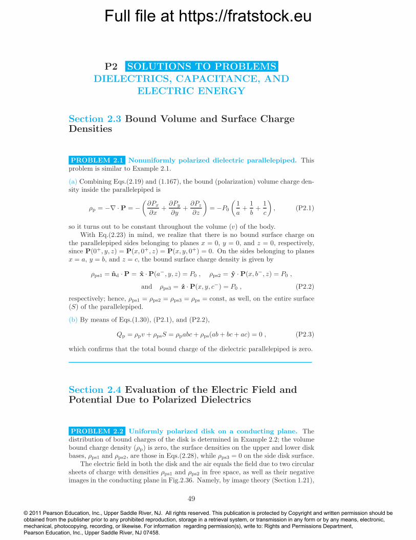
the charges (of density ρps2) right on the plane, at the coordinate z = 0+, and theirimages (of density −ρps2) right below the plane, at the coordinate z = 0−, canceleach other, so we are left with the two circular sheets of charge (in free space) shownin Fig.P2.1.
z
O
ae0
e0
rps1
-rps1
e0
e0
d
d
Figure P2.1 Two circular sheets of charge ρps1 = P and −ρps1 = −P in free space– equivalent, by virtue of image theory, to the uniformly polarized dielectric disk ona conducting plane in Fig.2.36.
Like in Eq.(2.29), we then invoke the superposition principle and the expressionfor the electric field due to a thin charged disk, Eq.(1.63), and obtain the totalelectric field vector at a point defined by the coordinate z (0 < z < ∞) along thez-axis in Fig.P2.1 (or Fig.2.36) as follows:
E = E1+E2 =P
2ε0
[
z − d|z − d| −
z − d√
a2 + (z − d)2− 1 +
z + d√
a2 + (z + d)2
]
z (z > 0) .
(P2.4)In the conductor in the original structure, Fig.2.36, there is no electric field, soE = 0 for z < 0.
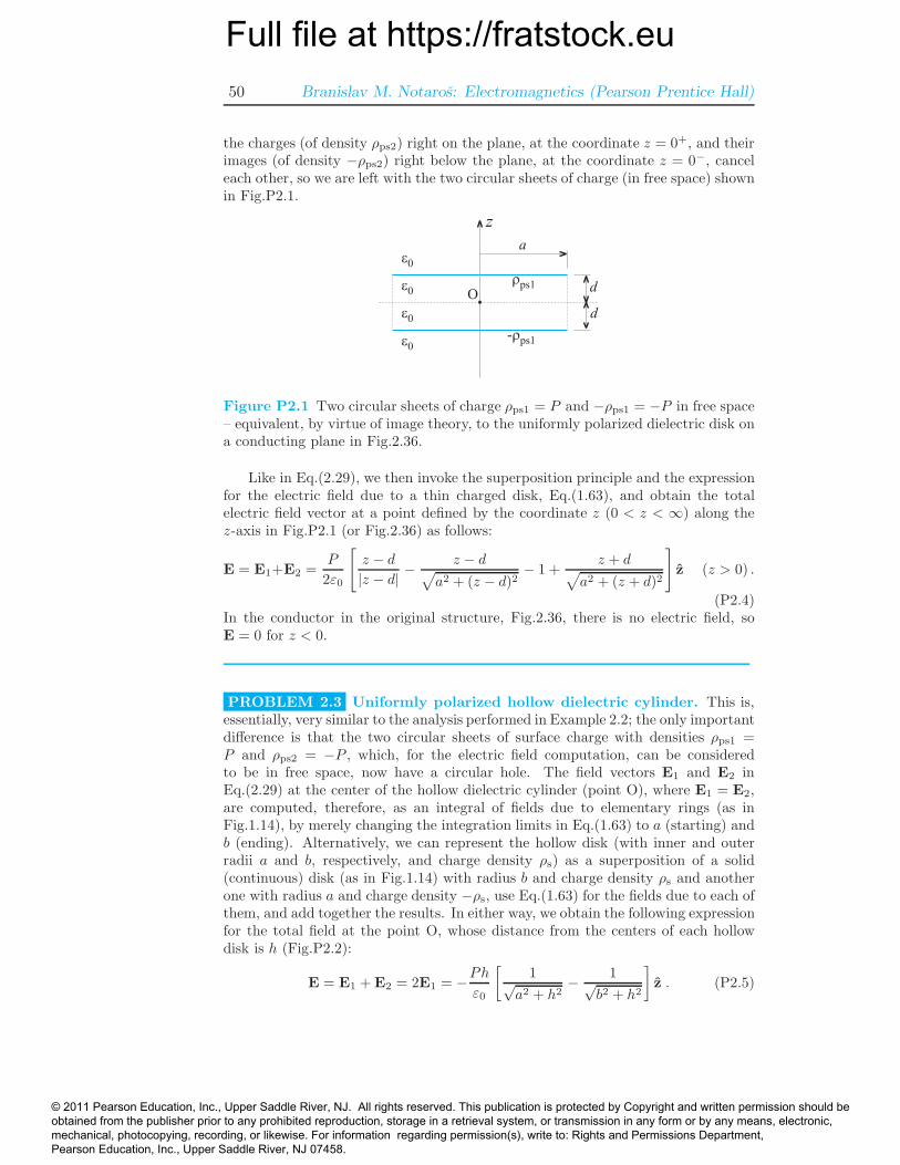
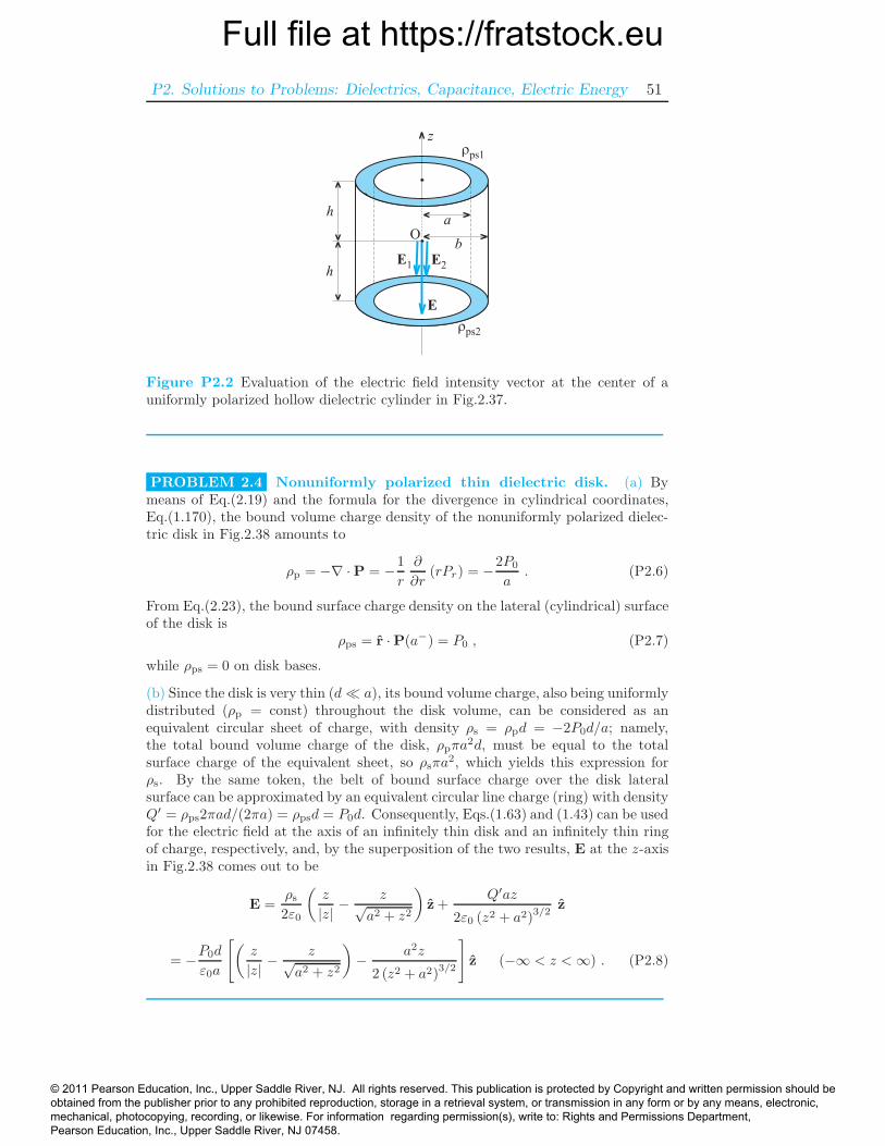
PROBLEM 2.3 Uniformly polarized hollow dielectric cylinder. This is,essentially, very similar to the analysis performed in Example 2.2; the only importantdifference is that the two circular sheets of surface charge with densities ρps1 =P and ρps2 = −P , which, for the electric field computation, can be consideredto be in free space, now have a circular hole. The field vectors E1 and E2 inEq.(2.29) at the center of the hollow dielectric cylinder (point O), where E1 = E2,are computed, therefore, as an integral of fields due to elementary rings (as inFig.1.14), by merely changing the integration limits in Eq.(1.63) to a (starting) andb (ending). Alternatively, we can represent the hollow disk (with inner and outerradii a and b, respectively, and charge density ρs) as a superposition of a solid(continuous) disk (as in Fig.1.14) with radius b and charge density ρs and anotherone with radius a and charge density −ρs, use Eq.(1.63) for the fields due to each ofthem, and add together the results. In either way, we obtain the following expressionfor the total field at the point O, whose distance from the centers of each hollowdisk is h (Fig.P2.2):
E = E1 + E2 = 2E1 = −Phε0
[1√
a2 + h2− 1√
b2 + h2
]
z . (P2.5)
© 2011 Pearson Education, Inc., Upper Saddle River, NJ. All rights reserved. This publication is protected by Copyright and written permission should be obtained from the publisher prior to any prohibited reproduction, storage in a retrieval system, or transmission in any form or by any means, electronic, mechanical, photocopying, recording, or likewise. For information regarding permission(s), write to: Rights and Permissions Department, Pearson Education, Inc., Upper Saddle River, NJ 07458.
Full file at https://fratstock.euP2. Solutions to Problems: Dielectrics, Capacitance, Electric Energy 51
O
z
a
b
h
hE1 E2
E
rps1
rps2
Figure P2.2 Evaluation of the electric field intensity vector at the center of auniformly polarized hollow dielectric cylinder in Fig.2.37.
PROBLEM 2.4 Nonuniformly polarized thin dielectric disk. (a) Bymeans of Eq.(2.19) and the formula for the divergence in cylindrical coordinates,Eq.(1.170), the bound volume charge density of the nonuniformly polarized dielec-tric disk in Fig.2.38 amounts to
ρp = −∇ ·P = −1
r
∂
∂r(rPr) = −2P0
a. (P2.6)
From Eq.(2.23), the bound surface charge density on the lateral (cylindrical) surfaceof the disk is
ρps = r ·P(a−) = P0 , (P2.7)
while ρps = 0 on disk bases.
(b) Since the disk is very thin (d≪ a), its bound volume charge, also being uniformlydistributed (ρp = const) throughout the disk volume, can be considered as anequivalent circular sheet of charge, with density ρs = ρpd = −2P0d/a; namely,the total bound volume charge of the disk, ρpπa
2d, must be equal to the totalsurface charge of the equivalent sheet, so ρsπa
2, which yields this expression forρs. By the same token, the belt of bound surface charge over the disk lateralsurface can be approximated by an equivalent circular line charge (ring) with densityQ′ = ρps2πad/(2πa) = ρpsd = P0d. Consequently, Eqs.(1.63) and (1.43) can be usedfor the electric field at the axis of an infinitely thin disk and an infinitely thin ringof charge, respectively, and, by the superposition of the two results, E at the z-axisin Fig.2.38 comes out to be
E =ρs
2ε0
(z
|z| −z√
a2 + z2
)
z +Q′az
2ε0 (z2 + a2)3/2z
= −P0d
ε0a
[(z
|z| −z√
a2 + z2
)
− a2z
2 (z2 + a2)3/2
]
z (−∞ < z <∞) . (P2.8)
© 2011 Pearson Education, Inc., Upper Saddle River, NJ. All rights reserved. This publication is protected by Copyright and written permission should be obtained from the publisher prior to any prohibited reproduction, storage in a retrieval system, or transmission in any form or by any means, electronic, mechanical, photocopying, recording, or likewise. For information regarding permission(s), write to: Rights and Permissions Department, Pearson Education, Inc., Upper Saddle River, NJ 07458.
Full file at https://fratstock.eu52 Branislav M. Notaros: Electromagnetics (Pearson Prentice Hall)
PROBLEM 2.5 Uniformly polarized dielectric hemisphere. (a) Thebound surface charge density at the bottom (flat) surface of the polarized hemi-sphere is that in Eqs.(2.28) – the second expression, and ρps at the upper (spherical)surface in Fig.2.39 is given by Eq.(2.30), so ρps = P cos θ, where now 0 ≤ θ ≤ π/2.
(b) We remove the conducting plane in Fig.2.39 using the image theory. The cir-cular sheet of bound surface charge right against the plane and its negative imagecancel each other. The hemispherical sheet, considered to be in a vacuum, is sup-plemented with another hemispherical sheet below the plane of symmetry, which isalso described by the function in Eq.(2.30), but with π/2 ≤ θ ≤ π (note that thefunction cos θ is antisymmetrical with respect to θ = π/2, which corresponds to anegative image of the charge, exactly as required by the image theory). We thusobtain the full spherical sheet of bound charge in Eq.(2.30), and conclude that thepolarized hemisphere on the conducting plane is equivalent to the polarized sphereof Fig.2.7, in free space. Hence, the electric field intensity vector at the point O inFig.2.39 is given by E = −P/(3ε0), Eq.(2.32).
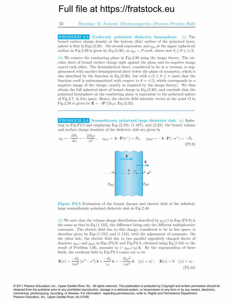
PROBLEM 2.6 Nonuniformly polarized large dielectric slab. (a) Refer-ring to Fig.P2.3 and employing Eqs.(2.19), (1.167), and (2.23), the bound volumeand surface charge densities of the dielectric slab are given by
ρp = −∂Px∂x
= −2P0x
a2, ρps1 = x ·P(a−) = P0 , ρps2 = − x ·P(−a+) = −P0 .
(P2.9)
rprps2
0 xa-a
rps1
x
E
P
Figure P2.3 Evaluation of the bound charges and electric field of the infinitelylarge nonuniformly polarized dielectric slab in Fig.2.40.
(b) We note that the volume charge distribution described by ρp(x) in Eqs.(P2.9) isthe same as that in Eq.(1.153), the difference being only the different multiplicativeconstants. The electric field due to this charge, considered to be in free space, istherefore given by Eqs.(1.155) and (1.154), with the adjustment of constants. Onthe other side, the electric field due to two parallel oppositely charged sheets ofdensities ρps1 and ρps2 in Eqs.(P2.9) and Fig.P2.3, obtained using Eq.(1.64) or theresult of Problem 1.60, amounts to (−ρps1/ε0) x. By the superposition of thesefields, the resultant field in Fig.P2.3 comes out to be
E(x) =−P0
ε0a2
(x2 − a2
)x +−P0
ε0x = −P0x
2
ε0a2x (|x| < a) ; E(x) = 0 (|x| > a) .
(P2.10)
© 2011 Pearson Education, Inc., Upper Saddle River, NJ. All rights reserved. This publication is protected by Copyright and written permission should be obtained from the publisher prior to any prohibited reproduction, storage in a retrieval system, or transmission in any form or by any means, electronic, mechanical, photocopying, recording, or likewise. For information regarding permission(s), write to: Rights and Permissions Department, Pearson Education, Inc., Upper Saddle River, NJ 07458.
Full file at https://fratstock.euP2. Solutions to Problems: Dielectrics, Capacitance, Electric Energy 53
(c) The voltage across the slab is
V =
∫ a
x=−aE(x) dx = − P0
ε0a2
∫ a
−ax2 dx = −2P0a
3ε0. (P2.11)
Section 2.5 Generalized Gauss’ Law
PROBLEM 2.7 Electric flux density vector. (a) Combining Eqs.(2.41) and(2.32), the electric flux density vector at the center (point O) of the polarizeddielectric sphere in Fig.2.7 turns out to be
D = ε0E + P = −P
3+ P =
2P
3. (P2.12)
(b) To find the vector D along the axis (z-axis) of the polarized dielectric disk lyingon a conducting plane in Fig.2.36, we apply Eq.(2.41) for points inside the dielectric,for 0 < z < d, where |z− d| = −(z− d) and (z− d)/|z− d| = −1 in the electric fieldexpression from Problem 2.2, and obtain
D = ε0E + P =P
2
[
− z − d√
a2 + (z − d)2+
z + d√
a2 + (z + d)2
]
. (P2.13)
For d < z < ∞ along the z-axis in Fig.2.36, P = 0 and D = ε0E (air), as wellas |z−d| = z−d in the electric field expression (Problem 2.2), which gives the sameexpression for D as in Eq.(P2.13), so it holds true for 0 < z <∞.
Finally, D = 0 for z < 0 (below the conducting plane).
PROBLEM 2.8 Total (free plus bound) volume charge density. (a) UsingEqs.(2.45), (2.19), and (2.41), the total (free plus bound) volume charge density inthe dielectric can, indeed, be expressed (in terms of the electric field intensity vector,E, only) as
ρtot = ρ+ ρp = ∇ ·D + (−∇ ·P) = ε0∇ ·E +∇ ·P−∇ ·P = ε0∇ · E . (P2.14)
(b) By means of the above expression and the formula for the divergence in Cartesiancoordinates, Eq.(1.167), ρtot for the given function E(x, y, z) comes out to be
ρtot = ε0
(∂Ex∂x
+∂Ey∂y
+∂Ez∂z
)
= 8.85(4yz − 3y2 + 3z2
)pC/m3 (y, z in m) .
(P2.15)
© 2011 Pearson Education, Inc., Upper Saddle River, NJ. All rights reserved. This publication is protected by Copyright and written permission should be obtained from the publisher prior to any prohibited reproduction, storage in a retrieval system, or transmission in any form or by any means, electronic, mechanical, photocopying, recording, or likewise. For information regarding permission(s), write to: Rights and Permissions Department, Pearson Education, Inc., Upper Saddle River, NJ 07458.
Full file at https://fratstock.eu54 Branislav M. Notaros: Electromagnetics (Pearson Prentice Hall)
PROBLEM 2.9 Uniform field in a dielectric. From the relationship ρ+ρp =ε0∇ · E (previous problem) and the fact that the divergence of the electric fieldvector in this dielectric region (E) is zero, since the field is uniform, the boundvolume charge density (ρp) in the region equals the negative of the free volumecharge density (ρ) at the same point, namely,
ρp = ε0∇ · E− ρ = −ρ (E = const) . (P2.16)
PROBLEM 2.10 Closed surface in a uniform field. Applying Gauss’ law,Eq.(1.133), to the closed surface S in Fig.2.41, over which the electric field vectoris constant (uniform electric field in the region), and can thus be taken out of theflux integral, and inside which there is no charge (charge-free region), we obtain
∮
S
E · dS =QSε0
−→ E ·∮
S
dS = 0 (E = const , QS = 0) . (P2.17)
We can rotate the parallel-plate capacitor in Fig.2.41, together with its (uniform)field, in an arbitrary way around the surface S, which is fixed, so that the vector(result of the integration)
∮
SdS does not change. Hence, the resulting relationship
in Eq.(P2.17) is satisfied (the dot product is zero) for an arbitrary direction of thevector E and a fixed vector
∮
SdS. This is possible only if
∮
S
dS = 0 , (P2.18)
which concludes our proof of this vector identity.
PROBLEM 2.11 Flux of the electric field intensity vector. With the useof Eqs.(2.41) and (2.44), the flux of E through a closed surface S situated entirelyinside the polarized dielectric body can be expressed as
ΨE =
∮
S
E · dS =1
ε0
(∮
S
D · dS−∮
S
P · dS
)
=1
ε0
(∫
v
ρ dv −∮
S
P · dS
)
,
(P2.19)where v denotes the volume enclosed by S.
Section 2.8 Electrostatic Field in Linear, Isotropic,and Homogeneous Media
PROBLEM 2.12 Total enclosed bound and free charge. CombiningEqs.(2.41), (2.47), (2.16), and (2.43), we obtain, similarly to Eqs.(2.60) and (2.61),the following relationship between the total bound charge QpS and free charge QS
© 2011 Pearson Education, Inc., Upper Saddle River, NJ. All rights reserved. This publication is protected by Copyright and written permission should be obtained from the publisher prior to any prohibited reproduction, storage in a retrieval system, or transmission in any form or by any means, electronic, mechanical, photocopying, recording, or likewise. For information regarding permission(s), write to: Rights and Permissions Department, Pearson Education, Inc., Upper Saddle River, NJ 07458.
Full file at https://fratstock.euP2. Solutions to Problems: Dielectrics, Capacitance, Electric Energy 55
enclosed by an imaginary closed surface S, via the permittivity ε of the homogeneousdielectric (ε = const):
P =ε− ε0ε
D −→∮
S
P · dS =ε− ε0ε
∮
S
D · dS −→ QpS = −ε− ε0ε
QS .
(P2.20)
PROBLEM 2.13 Charge-free homogeneous medium. That there is nobound volume charge in a homogeneous linear medium with no free volume chargeis obvious from Eq.(2.60):
ρ = 0 −→ ρp = −εr − 1
εrρ = 0 . (P2.21)
PROBLEM 2.14 Dielectric cylinder with free volume charge. This issimilar to Example 2.5 (dielectric sphere with free nonuniform volume charge).
(a) Applying the generalized Gauss’ law, Eq.(2.44), to the same cylindrical Gaussiansurface as in Problem 1.58 and Example 1.19, we obtain the following expressionfor the electric flux density in the dielectric cylinder with ρ = const:
D(r) 2πrh = ρ πr2h︸ ︷︷ ︸
v
−→ D(r) =ρr
2(0 ≤ r ≤ a) . (P2.22)
Having then in mind Eq.(2.47), the voltage between the axis and the surface of thecylinder amounts to
V =
∫ a
r=0
E(r) dr =1
εrε0
∫ a
0
D(r) dr =ρa2
4εrε0. (P2.23)
(b) As in Eqs.(2.67) and (2.68), the bound volume charge density inside the cylinderand surface charge density on its surface [note that the polarization vector is zerooutside the cylinder, Eq.(2.21)] are
ρp(r) = −εr − 1
εrρ (0 ≤ r < a) and ρps = P (a−) =
εr − 1
εrD(a−)
=ρ(εr − 1)a
2εr, (P2.24)
respectively.
PROBLEM 2.15 Linear-exponential volume charge distribution. (a) Forthe field (observation) points in the p-type region of the semiconductor in Fig.2.42,Eq.(2.74) now becomes
Ex(x) =ρ0
εa
∫ x
x′=−∞x′ ex
′/a dx′ = −ρ0a
ε
(
1− x
a
)
ex/a (−∞ < x ≤ 0) , (P2.25)
© 2011 Pearson Education, Inc., Upper Saddle River, NJ. All rights reserved. This publication is protected by Copyright and written permission should be obtained from the publisher prior to any prohibited reproduction, storage in a retrieval system, or transmission in any form or by any means, electronic, mechanical, photocopying, recording, or likewise. For information regarding permission(s), write to: Rights and Permissions Department, Pearson Education, Inc., Upper Saddle River, NJ 07458.
Full file at https://fratstock.eu56 Branislav M. Notaros: Electromagnetics (Pearson Prentice Hall)
where the integral is solved by integration by parts [∫x e−x dx = −(1+x) e−x+C].
Similarly, in the n-type region [see Eq.(2.75)] we have
Ex(x) =ρ0
εa
(∫ 0
−∞x′ ex
′/a dx′ +
∫ x
0
x′ e−x′/a dx′
)
= −ρ0a
ε
(
1 +x
a
)
e−x/a
(0 < x <∞) . (P2.26)
(b) Like in Eqs.(2.76) and (2.77), the potential at points in the p-type region inFig.2.42, for the reference point at the center of the junction (x = 0), is found as
V (x) =
∫ 0
x′=x
Ex(x′) dx′ = −ρ0a
ε
∫ 0
x
(
1− x′
a
)
ex′/a dx′
=ρ0a
ε
[
2a(
ex/a − 1)
− x ex/a]
(−∞ < x ≤ 0) , (P2.27)
and in the n-type region,
V (x) = −∫ x
0
Ex(x′) dx′ =
ρ0a
ε
∫ x
0
(
1 +x′
a
)
e−x′/a dx′
=ρ0a
ε
[
2a(
1− e−x/a)
− x e−x/a]
(0 < x <∞) . (P2.28)
(c) The voltage between the n-type and p-type ends (built-in voltage) of the pn
junction (diode) is
V (x→∞)− V (x→ −∞) =4ρ0a
2
ε. (P2.29)
Section 2.9 Dielectric-Dielectric BoundaryConditions
PROBLEM 2.16 Dielectric-dielectric boundary conditions. (a) From theboundary condition in Eq.(2.79), the tangential components of E1 and E2, namely,their x- and y-components, must be the same on the two sides of the boundary(plane z = 0), so
E2x = E1x = 4 V/m and E2y = E1y = −2 V/m . (P2.30)
As there is no free surface charge on the boundary, Eq.(2.83) gives the following forthe normal component (z-component) of E2 for z = 0−:
E2z = E2n =εr1εr2
E1n =εr1εr2
E1z = 10 V/m , (P2.31)
and hence
E2 = (4 x− 2 y + 10 z) V/m (ρs = 0) . (P2.32)
© 2011 Pearson Education, Inc., Upper Saddle River, NJ. All rights reserved. This publication is protected by Copyright and written permission should be obtained from the publisher prior to any prohibited reproduction, storage in a retrieval system, or transmission in any form or by any means, electronic, mechanical, photocopying, recording, or likewise. For information regarding permission(s), write to: Rights and Permissions Department, Pearson Education, Inc., Upper Saddle River, NJ 07458.
Full file at https://fratstock.euP2. Solutions to Problems: Dielectrics, Capacitance, Electric Energy 57
(b) Now ρs in the plane z = 0 is nonzero, and we use the boundary condition inEq.(2.85) in place of Eq.(P2.31),
ε1E1n − ε2E2n = ρs −→ E2z =1
εr2ε0(εr1ε0E1z − ρs) = 7 V/m , (P2.33)
which, combined with Eqs.(P2.30), results in
E2 = (4 x− 2 y + 7 z) V/m (ρs 6= 0) . (P2.34)
PROBLEM 2.17 Conductor-dielectric boundary conditions. Conductor-dielectric and conductor-free space boundary conditions in Eqs.(1.186), (2.58), and(1.190) are obtained from dielectric-dielectric boundary conditions in Eqs.(2.84) and(2.85) by specifying that E2 = 0 and D2 = 0 in the second medium (conductor) [seeEq.(1.181)] and D = εE or D = ε0E in the first medium (dielectric or free space).
PROBLEM 2.18 Water-air boundary. Marking water as medium 2 and air asmedium 1 in Fig.2.11, the law of refraction of the electric field lines at the water-airboundary in Eq.(2.87) gives
ε2 ≫ ε1 −→ ε1ε2≈ 0 −→ tanα1
tanα2≈ 0 −→ α1 ≈ 0 (α2 = 45◦) ,
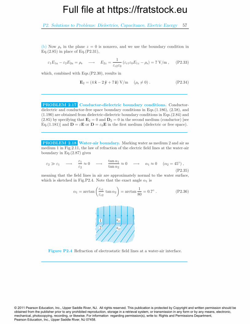
(P2.35)meaning that the field lines in air are approximately normal to the water surface,which is sketched in Fig.P2.4. Note that the exact angle α1 is
α1 = arctan
(εr1εr2
tanα2
)
= arctan1
80= 0.7◦ . (P2.36)
2
1
er2
er1
Figure P2.4 Refraction of electrostatic field lines at a water-air interface.
© 2011 Pearson Education, Inc., Upper Saddle River, NJ. All rights reserved. This publication is protected by Copyright and written permission should be obtained from the publisher prior to any prohibited reproduction, storage in a retrieval system, or transmission in any form or by any means, electronic, mechanical, photocopying, recording, or likewise. For information regarding permission(s), write to: Rights and Permissions Department, Pearson Education, Inc., Upper Saddle River, NJ 07458.
Full file at https://fratstock.eu58 Branislav M. Notaros: Electromagnetics (Pearson Prentice Hall)
Section 2.10 Poisson’s and Laplace’s Equations
PROBLEM 2.19 Poisson’s equation for inhomogeneous media. (a) Com-bining Eqs.(2.45), (2.47), and (1.101), we obtain the following second-order differ-ential equation:
∇ · (ε∇V ) = −ρ . (P2.37)
By means of the identity ∇· (fa) = f∇·a+(∇f) ·a (derived in Section 3.6), it canbe written also in the form
ε∇ · (∇V ) +∇V · ∇ε = −ρ −→ ∇2V +1
ε∇V · ∇ε = −ρ
ε, (P2.38)
which we refer to as Poisson’s equation for an inhomogeneous medium. On theother hand, if the dielectric medium is homogeneous, ε = const, so that ∇ε = 0,and this equation becomes Eq.(2.93), namely, the standard Poisson’s equation.
(b) The version of Eq.(P2.38) for a charge-free region (ρ = 0), that is, Laplace’sequation for an inhomogeneous medium, reads hence
∇2V +1
ε∇V · ∇ε = 0 , (P2.39)
which, in turn, reduces to the standard Laplace’s equation, Eq.(2.95), in the caseof a homogeneous medium.
PROBLEM 2.20 Vacuum diode. (a) We apply the one-dimensional Poisson’sequation in the x-coordinate, Eq.(2.98), from which the volume charge density inthe vacuum (ε = ε0) diode in Fig.2.43 amounts to
ρ(x) = −ε0d2V (x)
dx2= −4ε0V0x
−2/3
9d4/3(0 < x < d) . (P2.40)
(b)-(c) As in Eq.(2.101), the electric field intensity in the diode is given by
E(x) = −∇V = − dV (x)
dxx = −4V0x
1/3
3d4/3x (0 < x < d) . (P2.41)
Eq.(1.190) then tells us that the surface charge densities on the cathode and anode(Fig.2.43) are
ρs1 = ε0 x · E(0+) = 0 and ρs2 = ε0(− x) · E(d−) =4ε0V0
3d, (P2.42)
respectively.
(d) Performing a similar integration as in Eq.(1.149) and using the second expressionin Eqs.(1.30), the total charge of the diode turns out to be
Q =
∫
v
ρ(x)S dx︸︷︷︸
dv
+ρs1S + ρs2S = −4ε0V0S
9d4/3
∫ d
x=0
x−2/3 dx+4ε0V0S
3d= 0 , (P2.43)
© 2011 Pearson Education, Inc., Upper Saddle River, NJ. All rights reserved. This publication is protected by Copyright and written permission should be obtained from the publisher prior to any prohibited reproduction, storage in a retrieval system, or transmission in any form or by any means, electronic, mechanical, photocopying, recording, or likewise. For information regarding permission(s), write to: Rights and Permissions Department, Pearson Education, Inc., Upper Saddle River, NJ 07458.
Full file at https://fratstock.euP2. Solutions to Problems: Dielectrics, Capacitance, Electric Energy 59
where S stands for the (inner) surface area of the cathode or anode in Fig.2.43.
PROBLEM 2.21 Application of Poisson’s equation in spherical coordi-nates. This is similar to the application of Poisson’s equation in Cartesian coordi-nates in Example 2.7.
(a) Because of the spherical symmetry of the problem, the electric potential dependsonly on the radial spherical coordinate r, so that the formula for the Laplacian inspherical coordinates, Eq.(2.97), retains only the first term. Combining this formulawith Poisson’s equation, Eq.(2.93), we have
∇2V =1
r2d
dr
(
r2dV
dr
)
= −ρ(r)ε0
= −ρ0r
ε0a(a < r < b) , (P2.44)
and the resulting second-order differential equation in r is solved by two integrations,like in Eq.(2.99), as follows:
r2dV
dr=
∫ (
−ρ0r3
ε0a
)
dr = −ρ0r4
4ε0a+ C1 −→ V (r) =
∫ (
−ρ0r2
4ε0a+C1
r2
)
dr
= − ρ0r3
12ε0a− C1
r+ C2 . (P2.45)
The integration constants, C1 and C2, are computed from the boundary conditionsat the surfaces of metallic electrodes,
V (a) = −ρ0a2
12ε0− C1
a+ C2 = V0 and V (b) = − ρ0b
3
12ε0a− C1
b+ C2 = 0 . (P2.46)
Substituting the numerical data (note that ρ0 = 3 µC/m3), the two equations (intwo unknowns, C1 and C2) become
−100C1 + C2 = 12.82 and − 20C1 + C2 = 352.9 (C1 in V ·m; C2 in V) ,(P2.47)
and their solution is C1 = 4.251 V ·m and C2 = 438 V. Hence, the potential atan arbitrary point between the electrodes, for a < r < b, given with respect to theouter electrode, which is at zero potential, comes out to be
V (r) =
(
−2.823× 10⁶r3 − 4.251
r+ 438
)
V (r in m) . (P2.48)
(b) In the same way as in Eq.(P1.81), we obtain the electric field vector betweenthe electrodes (a < r < b) from the result for V in Eq.(P2.48):
E(r) = −∇V = − dV
drr =
(
8.47× 10⁶r2 − 4.251
r2
)
r V/m (r in m) . (P2.49)
PROBLEM 2.22 Application of Laplace’s equation in spherical coordi-nates. Since ρ = 0 between the electrodes, we are now solving the one-dimensionalLaplace’s equation in the radial spherical coordinate r,
∇2V =1
r2d
dr
(
r2dV
dr
)
= 0 (a < r < b) , (P2.50)
© 2011 Pearson Education, Inc., Upper Saddle River, NJ. All rights reserved. This publication is protected by Copyright and written permission should be obtained from the publisher prior to any prohibited reproduction, storage in a retrieval system, or transmission in any form or by any means, electronic, mechanical, photocopying, recording, or likewise. For information regarding permission(s), write to: Rights and Permissions Department, Pearson Education, Inc., Upper Saddle River, NJ 07458.
Full file at https://fratstock.eu60 Branislav M. Notaros: Electromagnetics (Pearson Prentice Hall)
and the two integrations result in
r2dV
dr= C1 −→ V (r) =
∫C1
r2dr = −C1
r+ C2 . (P2.51)
From the boundary conditions,
V (a) = −C1
a+ C2 = V0 and V (b) = −C1
b+ C2 = 0 , (P2.52)
and hence C1 = −0.125 V ·m and C2 = −2.5 V, with which the solution for thepotential in Eq.(P2.51) becomes
V (r) =
(0.125
r− 2.5
)
V (r in m) . (P2.53)
(b) The electric field for a < r < b is given by
E(r) = − dV
drr =
0.125
r2r V/m (r in m) . (P2.54)
Section 2.11 Finite-Difference Method forNumerical Solution of Laplace’s Equation
PROBLEM 2.23 FD computer program – iterative solution. Computerprogram for the finite-difference analysis of the coaxial cable of square cross section(Fig.2.13) based on Eq.(2.107) is given in the associated MATLAB exercise.
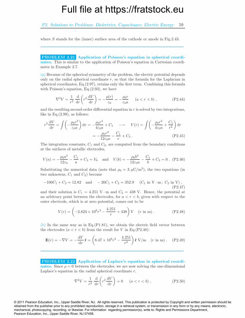
(a) Simulation results for the distribution of the potential and the electric fieldintensity in the space between the conductors and for the charge distribution of theconductors of the square coaxial cable, taking the grid spacing to be d = a/10 andthe tolerance of the potential δV = 0.001 V, are shown in Fig.P2.5.
(b) The computed total charges per unit length of the inner and outer conductors ofthe cable [Eq.(2.111)], taking d = a/N and N = 2, 3, 5, 7, 9, 10, and 12, respectively,are tabulated in Table P2.1.
Table P2.1 Total charges p.u.l. of theinner and outer conductors of the squarecoaxial cable in Fig.2.13.
N Qinner[ C] Qouter[ C]
2 1.0625 × 10⁻¹⁰ −1.2103 × 10⁻¹⁰
3 1.0261 × 10⁻¹⁰ −1.1642 × 10⁻¹⁰
5 1.0219 × 10⁻¹⁰ −1.1374 × 10⁻¹⁰
7 1.0260 × 10⁻¹⁰ −1.1331 × 10⁻¹⁰
9 1.0281 × 10⁻¹⁰ −1.1380 × 10⁻¹⁰
10 1.0282 × 10⁻¹⁰ −1.1423 × 10⁻¹⁰
12 1.0265 × 10⁻¹⁰ −1.1544 × 10⁻¹⁰
© 2011 Pearson Education, Inc., Upper Saddle River, NJ. All rights reserved. This publication is protected by Copyright and written permission should be obtained from the publisher prior to any prohibited reproduction, storage in a retrieval system, or transmission in any form or by any means, electronic, mechanical, photocopying, recording, or likewise. For information regarding permission(s), write to: Rights and Permissions Department, Pearson Education, Inc., Upper Saddle River, NJ 07458.
Full file at https://fratstock.euP2. Solutions to Problems: Dielectrics, Capacitance, Electric Energy 61
0
0.01
0.02
0.03
0
0.01
0.02
0.03−1
−0.5
0
0.5
1
x
Potential distribution for N = 10, iterative FD method
y −1
−0.8
−0.6
−0.4
−0.2
0
0.2
0.4
0.6
0.8
1
0 0.005 0.01 0.015 0.02 0.025 0.030
0.005
0.01
0.015
0.02
0.025
0.03
x
y
Electric field intensity vector at each node for N = 10, iterative FD method
0.2
z [cm]
0.4 0.6 0.8 10
0.5
1
1.5
2
2.5
30.5 1 1.5 2 2.5 3
-1.6
-1.2
-0.8
-0.4
0
z [cm]
rs [nC/m ]2
rs [nC/m ]2
inner conductor outer conductor
Figure P2.5 Electric potential and field intensity in the space between the con-ductors, and the surface charge density on the surfaces of conductors, of the coaxialcable of square cross section in Fig.2.13 – results by the iterative finite-differencetechnique [Eqs.(2.107)-(2.110)] (FD computer program is provided in the associatedMATLAB exercise).
PROBLEM 2.24 FD computer program – direct solution. Computer pro-gram for the finite-difference analysis of a square coaxial cable by directly solvingthe system of linear algebraic equations with the potentials at interior grid nodesin Fig.2.13(b) as unknowns is provided in the associated MATLAB exercise.
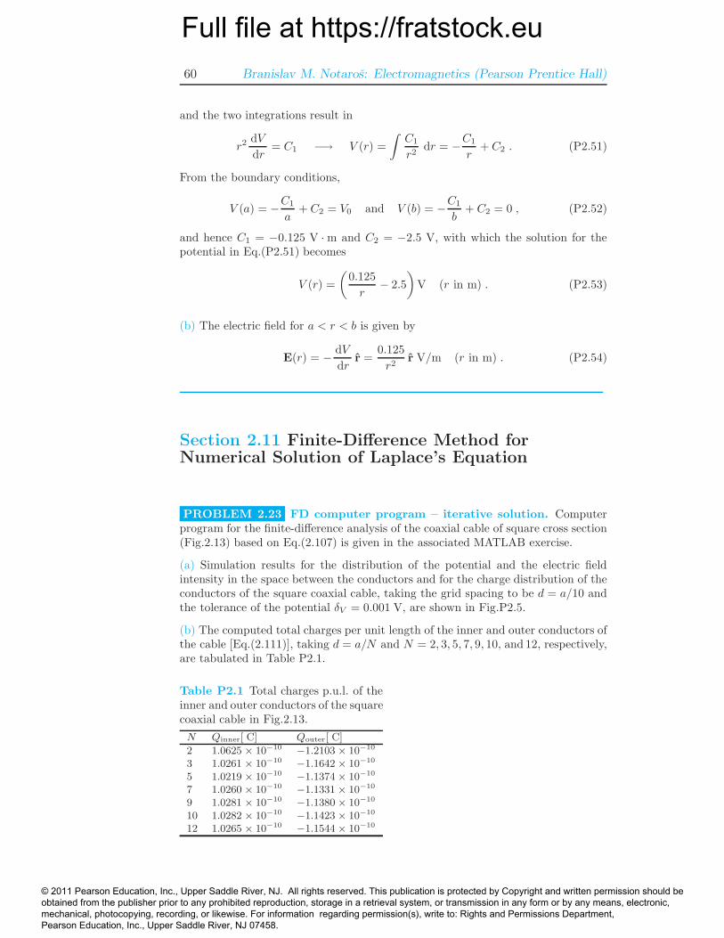
(a) The computed potential, field, and charge distributions, using the direct FDtechnique, are shown in Fig.P2.6. A good agreement with the results by the iterativeFD technique (previous problem) is observed.
(b) Table P2.2 contains the results, obtained by the direct FD technique, for the
© 2011 Pearson Education, Inc., Upper Saddle River, NJ. All rights reserved. This publication is protected by Copyright and written permission should be obtained from the publisher prior to any prohibited reproduction, storage in a retrieval system, or transmission in any form or by any means, electronic, mechanical, photocopying, recording, or likewise. For information regarding permission(s), write to: Rights and Permissions Department, Pearson Education, Inc., Upper Saddle River, NJ 07458.
Full file at https://fratstock.eu62 Branislav M. Notaros: Electromagnetics (Pearson Prentice Hall)
0
0.01
0.02
0.03
0
0.01
0.02
0.03−1
−0.5
0
0.5
1
x
Potential distribution for N = 10, direct FD method
y −1
−0.8
−0.6
−0.4
−0.2
0
0.2
0.4
0.6
0.8
1
0 0.005 0.01 0.015 0.02 0.025 0.030
0.005
0.01
0.015
0.02
0.025
0.03
x
y
Electric field intensity vector at each node for N = 10, direct FD method
rs [nC/m ]2
rs [nC/m ]2
inner conductor outer conductor
0.5
1
1.5
2
2.5
3
0.2
z [cm]
0.4 0.6 0.8 10
-1.6
-1.2
-0.8
-0.4
z [cm]
0.5 1 1.5 2 2.5 30
Figure P2.6 Electric potential, field, and charge distributions of the square coax-ial cable in Fig.2.13 – results by the direct finite-difference technique (computerprogram is given in the associated MATLAB exercise).
total charges per unit length of the inner and outer conductors of the cable.
Table P2.2 Total p.u.l. charges of ca-ble conductors obtained by the directFD technique.
N Qinner[ C] Qouter[ C]
2 1.0625 × 10⁻¹⁰ −1.2101 × 10⁻¹⁰
3 1.0267 × 10⁻¹⁰ −1.1620 × 10⁻¹⁰
5 1.0244 × 10⁻¹⁰ −1.1308 × 10⁻¹⁰
7 1.0317 × 10⁻¹⁰ −1.1197 × 10⁻¹⁰
9 1.0384 × 10⁻¹⁰ −1.1142 × 10⁻¹⁰
10 1.0414 × 10⁻¹⁰ −1.1124 × 10⁻¹⁰
12 1.0464 × 10⁻¹⁰ −1.1098 × 10⁻¹⁰
© 2011 Pearson Education, Inc., Upper Saddle River, NJ. All rights reserved. This publication is protected by Copyright and written permission should be obtained from the publisher prior to any prohibited reproduction, storage in a retrieval system, or transmission in any form or by any means, electronic, mechanical, photocopying, recording, or likewise. For information regarding permission(s), write to: Rights and Permissions Department, Pearson Education, Inc., Upper Saddle River, NJ 07458.
Full file at https://fratstock.euP2. Solutions to Problems: Dielectrics, Capacitance, Electric Energy 63
Section 2.13 Analysis of Capacitors withHomogeneous Dielectrics
PROBLEM 2.25 Capacitance of the earth. Using Eq.(2.121), the capaci-tance of the earth turns out to be
Cearth = 4πε0R = 709.6 µF (R = 6378 km) . (P2.55)
PROBLEM 2.26 Capacitance of a person. Taking the diameters of theinscribed and overscribed spheres to be 2Rmin = 30 cm and 2Rmax = 170 cm,respectively (note that these adopted dimensions are completely arbitrary, and arejust meant to be illustrative of an estimated value of the capacitance), that is,Rmin = 15 cm and Rmax = 85 cm, we have 4πε0Rmin = 16.7 pF and 4πε0Rmax =94.6 pF. Therefore, the capacitance of an average human body can be estimated tobe within the range 16.7 pF < C < 94.6 pF.
PROBLEM 2.27 Capacitance of a metallic cube, computed by theMoM. The capacitance of the metallic cube numerically analyzed by the methodof moments in Problem 1.85 amounts to C = Q/V0 = 73.27 pF. The capacitancesof the metallic sphere [Eq.(2.119)] inscribed in the cube (sphere radius ra = a/2),the sphere overscribed about the cube (rb = a
√3/2), the one with rc = (ra + rb)/2,
the sphere having the same surface as the cube [rd = a√
3/(2π)], and that withthe same volume as the cube {re = a[3/(4π)]1/3} come out to be Ca = 55.63 pF,Cb = 96.36 pF, Cc = 76 pF, Cd = 76.88 pF, and Ce = 69.02 pF, respectively. Wesee that the capacitance of the sphere whose radius equals the arithmetic mean ofthe radii of spheres inscribed in and overscribed about the cube (Cc = 76 pF) isquite close in value to the capacitance of the cube.
PROBLEM 2.28 RG-55/U coaxial cable. Using Eq.(2.123), the capacitanceper unit length of the RG-55/U coaxial cable amounts to C′ = 2πεrε0/ ln(b/a) =70 pF/m.
PROBLEM 2.29 Capacitance p.u.l. of a square coaxial cable, FD anal-ysis. The capacitance per unit length of the coaxial cable of square cross sectionin Fig.2.13 numerically analyzed by the finite-difference technique presented in Sec-tion 2.11 is obtained to be Citerative = 51.41 pF/m by the iterative FD technique(Problem 2.23) and Cdirect = 52.07 pF/m by the direct FD technique (Problem2.24), with the tolerance of the potential of δV = 0.001 V in the iterative solutionand the grid spacing of d = a/10 in both solutions. As a reference, the per-unit-length capacitance of a (standard) coaxial cable (of circular cross section) having
© 2011 Pearson Education, Inc., Upper Saddle River, NJ. All rights reserved. This publication is protected by Copyright and written permission should be obtained from the publisher prior to any prohibited reproduction, storage in a retrieval system, or transmission in any form or by any means, electronic, mechanical, photocopying, recording, or likewise. For information regarding permission(s), write to: Rights and Permissions Department, Pearson Education, Inc., Upper Saddle River, NJ 07458.
Full file at https://fratstock.eu64 Branislav M. Notaros: Electromagnetics (Pearson Prentice Hall)
the same ratio of conductor radii (b/a = 3) and dielectric (air) as the square cableis Cstandard coax = 50.61 pF/m [from Eq.(2.123)].
PROBLEM 2.30 Parallel-plate capacitor model of a thundercloud.Based on Eqs.(2.127) and (2.126), the capacitance of the parallel-plate capacitor ap-proximating a thundercloud, the voltage between the top and bottom of the cloud,and the electric field intensity in the cloud come out to be C = ε0S/d = 132.8 nF,V = Q/C = 2.26 GV, and E = V/d = 2.26 MV/m, respectively.
PROBLEM 2.31 MoM numerical analysis of a parallel-plate capacitor.Computer program based on the method of moments for the analysis of the parallel-plate capacitor in Fig.2.19 is given in the associated MATLAB exercise. Using theMoM program, the capacitance (C) of this capacitor for d/a ratios of 0.1, 0.5, 1, 2,and 10 is found to be 117 pF, 38.3 pF, 28.7 pF, 24 pF, and 20.6 pF, respectively.The corresponding C values obtained from Eq.(2.127), which neglects the fringingeffects, turn out to be 88.5 pF, 17.7 pF, 8.85 pF, 4.43 pF, and 0.885 pF.
PROBLEM 2.32 Nonsymmetrical thin two-wire line. The only differencewith respect to the analysis of a symmetrical thin two-wire transmission line in air,Fig.2.22, is the upper integration limit in computing the voltage between the lineconductors. Incorporating this change in Eqs.(2.140) and (2.141), we obtain thefollowing expression for the capacitance per unit length of a nonsymmetrical thintwo-wire line:
V =
∫ d−b
x=a
E dx =Q′
2πε0
[∫ d−b
a
dx
x−∫ d−b
a
d(d− x)d− x
]
=Q′
2πε0
[
lnx|d−ba − ln(d− x)|d−ba
]
=Q′
2πε0
(
lnd− ba− ln
b
d− a
)
=Q′
2πε0ln
(d− a)(d − b)ab
≈ Q′
2πε0lnd2
ab−→ C′ =
Q′
V≈ πε0
ln(d/√ab)
(P2.56)
(since d− a ≈ d and d− b ≈ d).Similarly, we can pursue an alternative way of obtaining C′ based on Eq.(1.197),
as in Eqs.(2.142) and (2.143), which now become
VM1 =Q′
2πε0lnd− ba
+−Q′
2πε0ln
b
d− a −→ C′ =Q′
VM1
≈ πε0
ln(d/√ab)
. (P2.57)
Of course, for a = b, the result for C′ in Eq.(P2.56) or (P2.57) reduces to thatin Eq.(2.141).
PROBLEM 2.33 Thick symmetrical two-wire line. The capacitance perunit length of a (thick or thin) symmetrical two-wire line with the wire distance to
© 2011 Pearson Education, Inc., Upper Saddle River, NJ. All rights reserved. This publication is protected by Copyright and written permission should be obtained from the publisher prior to any prohibited reproduction, storage in a retrieval system, or transmission in any form or by any means, electronic, mechanical, photocopying, recording, or likewise. For information regarding permission(s), write to: Rights and Permissions Department, Pearson Education, Inc., Upper Saddle River, NJ 07458.
Full file at https://fratstock.euP2. Solutions to Problems: Dielectrics, Capacitance, Electric Energy 65
radius ratio d/a in air computed using the two expressions,
C′1 =
πε0
ln{d/(2a) +√
[d/(2a)]2 − 1}and C′
2 =πε0
ln(d/a), (P2.58)
for different values of d/a are given in Table P2.3. We see that the results obtainedwith the thin-wire approximation of the line (C′
2) are quite accurate for d/a ≥ 10,and are acceptable even for d/a ≥ 5.
Table P2.3 Capacitance p.u.l. of a two-wireline computed by expressions in Eqs.(P2.58).
d/a C′
1 (pF/m) C′
2 (pF/m) Error (%)
3 28.9 25.32 14.155 17.754 17.283 2.7210 12.134 12.08 0.44320 9.2931 9.2853 0.084100 6.04036 6.04023 0.0022
PROBLEM 2.34 Two small metallic spheres in air. The capacitor consist-ing of two small metallic spheres in air can be analyzed as the thin two-wire linein Fig.2.22, by just changing the field dependence Q′/(2πε0r) to Q/(4πε0r
2). Withthis, Eq.(2.139) becomes
E = E1 + E2 =Q
4πε0
[1
x2+
1
(d− x)2]
, (P2.59)
and the voltage of the capacitor is, in place of Eq.(2.140), found as
V =
∫ d−a
x=a
E dx =Q
4πε0
[∫ d−a
a
dx
x2−∫ d−a
a
d(d− x)(d − x)2
]
=Q
4πε0
[1
a− 1
d− a −(
1
d− a −1
a
)]
=Q
2πε0
(1
a− 1
d− a
)
≈ Q
2πε0a(d≫ a) .
(P2.60)Its capacitance is
C =Q
V= 2πε0a . (P2.61)
Note that, since d ≫ a, the voltage between the two spheres can alternativelybe obtained using the expression for the potential of an isolated metallic sphere,Eq.2.120, twice. Namely, V can be computed as the voltage from the first sphere(with charge Q) to the reference point for potential (at infinity) plus the voltagefrom the reference point to the second sphere (the one with charge −Q), where thetwo voltages equal the potential (with respect to infinity) of the first sphere and thenegative of the potential of the second sphere, respectively, so that
V = Vsphere with Q + (−Vsphere with −Q) =Q
4πε0a+
(
− −Q4πε0a
)
=Q
2πε0a. (P2.62)
© 2011 Pearson Education, Inc., Upper Saddle River, NJ. All rights reserved. This publication is protected by Copyright and written permission should be obtained from the publisher prior to any prohibited reproduction, storage in a retrieval system, or transmission in any form or by any means, electronic, mechanical, photocopying, recording, or likewise. For information regarding permission(s), write to: Rights and Permissions Department, Pearson Education, Inc., Upper Saddle River, NJ 07458.
Full file at https://fratstock.eu66 Branislav M. Notaros: Electromagnetics (Pearson Prentice Hall)
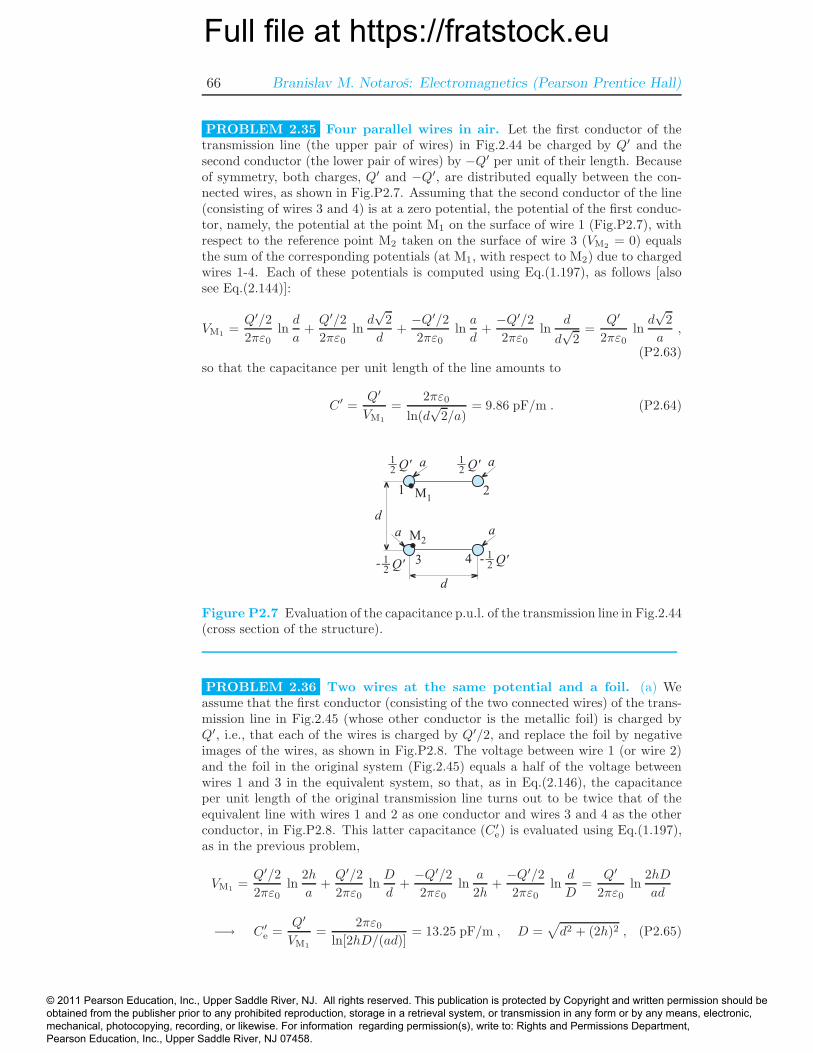
PROBLEM 2.35 Four parallel wires in air. Let the first conductor of thetransmission line (the upper pair of wires) in Fig.2.44 be charged by Q′ and thesecond conductor (the lower pair of wires) by −Q′ per unit of their length. Becauseof symmetry, both charges, Q′ and −Q′, are distributed equally between the con-nected wires, as shown in Fig.P2.7. Assuming that the second conductor of the line(consisting of wires 3 and 4) is at a zero potential, the potential of the first conduc-tor, namely, the potential at the point M1 on the surface of wire 1 (Fig.P2.7), withrespect to the reference point M2 taken on the surface of wire 3 (VM2 = 0) equalsthe sum of the corresponding potentials (at M1, with respect to M2) due to chargedwires 1-4. Each of these potentials is computed using Eq.(1.197), as follows [alsosee Eq.(2.144)]:
VM1 =Q′/2
2πε0lnd
a+Q′/2
2πε0lnd√
2
d+−Q′/2
2πε0lna
d+−Q′/2
2πε0ln
d
d√
2=
Q′
2πε0lnd√
2
a,
(P2.63)so that the capacitance per unit length of the line amounts to
C′ =Q′
VM1
=2πε0
ln(d√
2/a)= 9.86 pF/m . (P2.64)
Q'-_12
M2
d
d
a a
a a
1 2
3 4
M1
Q'_12 Q'
_12
Q'-_12
Figure P2.7 Evaluation of the capacitance p.u.l. of the transmission line in Fig.2.44(cross section of the structure).
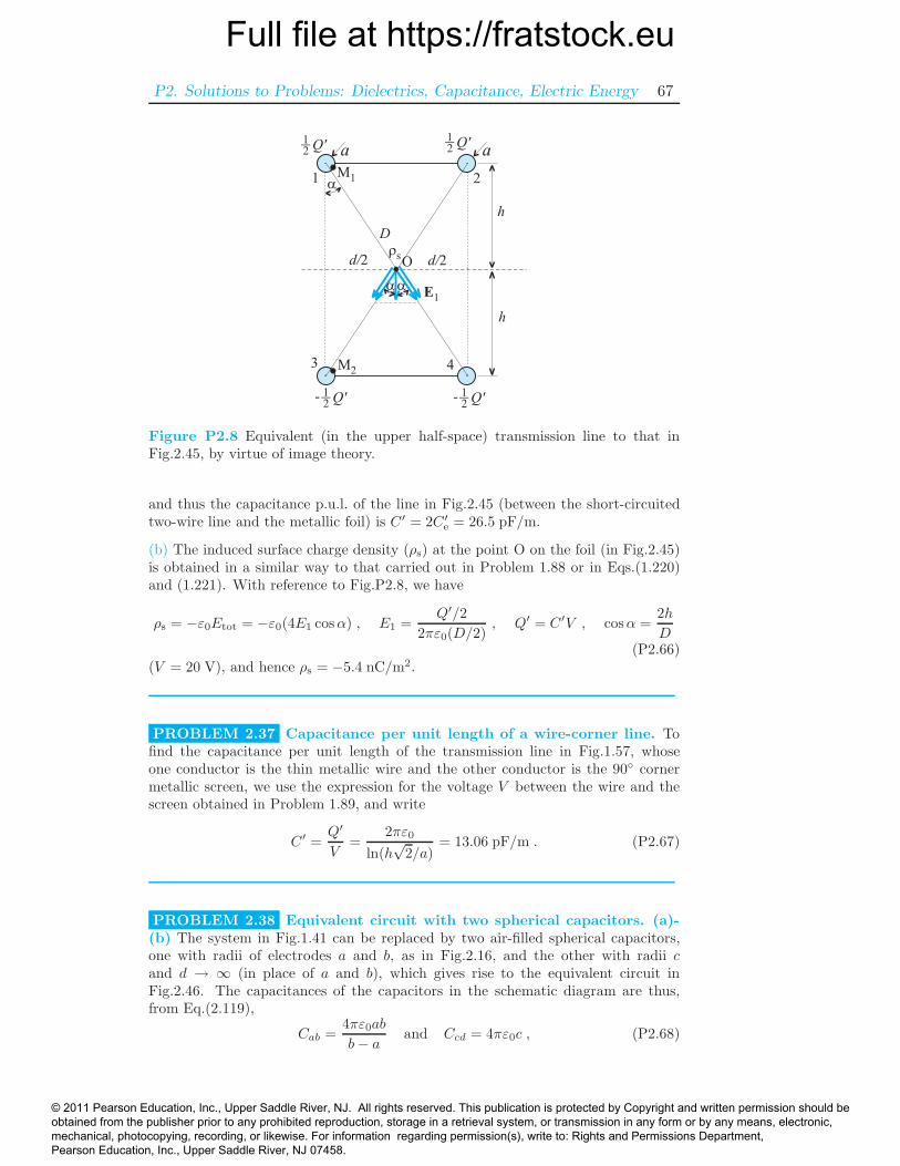
PROBLEM 2.36 Two wires at the same potential and a foil. (a) Weassume that the first conductor (consisting of the two connected wires) of the trans-mission line in Fig.2.45 (whose other conductor is the metallic foil) is charged byQ′, i.e., that each of the wires is charged by Q′/2, and replace the foil by negativeimages of the wires, as shown in Fig.P2.8. The voltage between wire 1 (or wire 2)and the foil in the original system (Fig.2.45) equals a half of the voltage betweenwires 1 and 3 in the equivalent system, so that, as in Eq.(2.146), the capacitanceper unit length of the original transmission line turns out to be twice that of theequivalent line with wires 1 and 2 as one conductor and wires 3 and 4 as the otherconductor, in Fig.P2.8. This latter capacitance (C′
e) is evaluated using Eq.(1.197),as in the previous problem,
VM1 =Q′/2
2πε0ln
2h
a+Q′/2
2πε0lnD
d+−Q′/2
2πε0ln
a
2h+−Q′/2
2πε0lnd
D=
Q′
2πε0ln
2hD
ad
−→ C′e =
Q′
VM1
=2πε0
ln[2hD/(ad)]= 13.25 pF/m , D =
√
d2 + (2h)2 , (P2.65)
© 2011 Pearson Education, Inc., Upper Saddle River, NJ. All rights reserved. This publication is protected by Copyright and written permission should be obtained from the publisher prior to any prohibited reproduction, storage in a retrieval system, or transmission in any form or by any means, electronic, mechanical, photocopying, recording, or likewise. For information regarding permission(s), write to: Rights and Permissions Department, Pearson Education, Inc., Upper Saddle River, NJ 07458.
Full file at https://fratstock.euP2. Solutions to Problems: Dielectrics, Capacitance, Electric Energy 67
Q'-_12
M2
M1
Q'_12
Q'_12
Q'-_12
h
d/2 d/2
a a
O
1 2
h
3 4
rs
aa
D
E1
a
Figure P2.8 Equivalent (in the upper half-space) transmission line to that inFig.2.45, by virtue of image theory.
and thus the capacitance p.u.l. of the line in Fig.2.45 (between the short-circuitedtwo-wire line and the metallic foil) is C′ = 2C′
e = 26.5 pF/m.
(b) The induced surface charge density (ρs) at the point O on the foil (in Fig.2.45)is obtained in a similar way to that carried out in Problem 1.88 or in Eqs.(1.220)and (1.221). With reference to Fig.P2.8, we have
ρs = −ε0Etot = −ε0(4E1 cosα) , E1 =Q′/2
2πε0(D/2), Q′ = C′V , cosα =
2h
D(P2.66)
(V = 20 V), and hence ρs = −5.4 nC/m2.
PROBLEM 2.37 Capacitance per unit length of a wire-corner line. Tofind the capacitance per unit length of the transmission line in Fig.1.57, whoseone conductor is the thin metallic wire and the other conductor is the 90◦ cornermetallic screen, we use the expression for the voltage V between the wire and thescreen obtained in Problem 1.89, and write
C′ =Q′
V=
2πε0
ln(h√
2/a)= 13.06 pF/m . (P2.67)
PROBLEM 2.38 Equivalent circuit with two spherical capacitors. (a)-(b) The system in Fig.1.41 can be replaced by two air-filled spherical capacitors,one with radii of electrodes a and b, as in Fig.2.16, and the other with radii cand d → ∞ (in place of a and b), which gives rise to the equivalent circuit inFig.2.46. The capacitances of the capacitors in the schematic diagram are thus,from Eq.(2.119),
Cab =4πε0ab
b− a and Ccd = 4πε0c , (P2.68)
© 2011 Pearson Education, Inc., Upper Saddle River, NJ. All rights reserved. This publication is protected by Copyright and written permission should be obtained from the publisher prior to any prohibited reproduction, storage in a retrieval system, or transmission in any form or by any means, electronic, mechanical, photocopying, recording, or likewise. For information regarding permission(s), write to: Rights and Permissions Department, Pearson Education, Inc., Upper Saddle River, NJ 07458.
Full file at https://fratstock.eu68 Branislav M. Notaros: Electromagnetics (Pearson Prentice Hall)
where Ccd can also be obtained from Eq.(2.121), as the capacitance of an isolatedmetallic sphere of radius c in air.
(c) The charge of the first (left) electrode of the first capacitor (of capacitance Cab)in Fig.2.46 equals the charge of the metallic sphere in Fig.1.41, so Qa = Q. Thecharge of the second electrode of this capacitor is opposite, hence Qb = −Qa =−Q. Since the metallic shell in Fig.1.41 is uncharged, and it is represented by thesecond electrode of the first capacitor and first electrode of the second capacitor (ofcapacitance Ccd) in the equivalent circuit, we have Qb+Qc = 0 and Qc = −Qb = Qin Fig.2.46, and then Qd = −Qc = −Q for the second capacitor.
From Fig.2.46, the potential at the point O in Fig.1.41, that is, the potential ofthe metallic sphere, can be obtained, using Eqs.(2.113) and (P2.68), as
V = Vab + Vcd =QaCab
+QcCcd
=Q(bc− ac+ ab)
4πε0abc, (P2.69)
which, of course, is the same result as in Eq.(1.202).
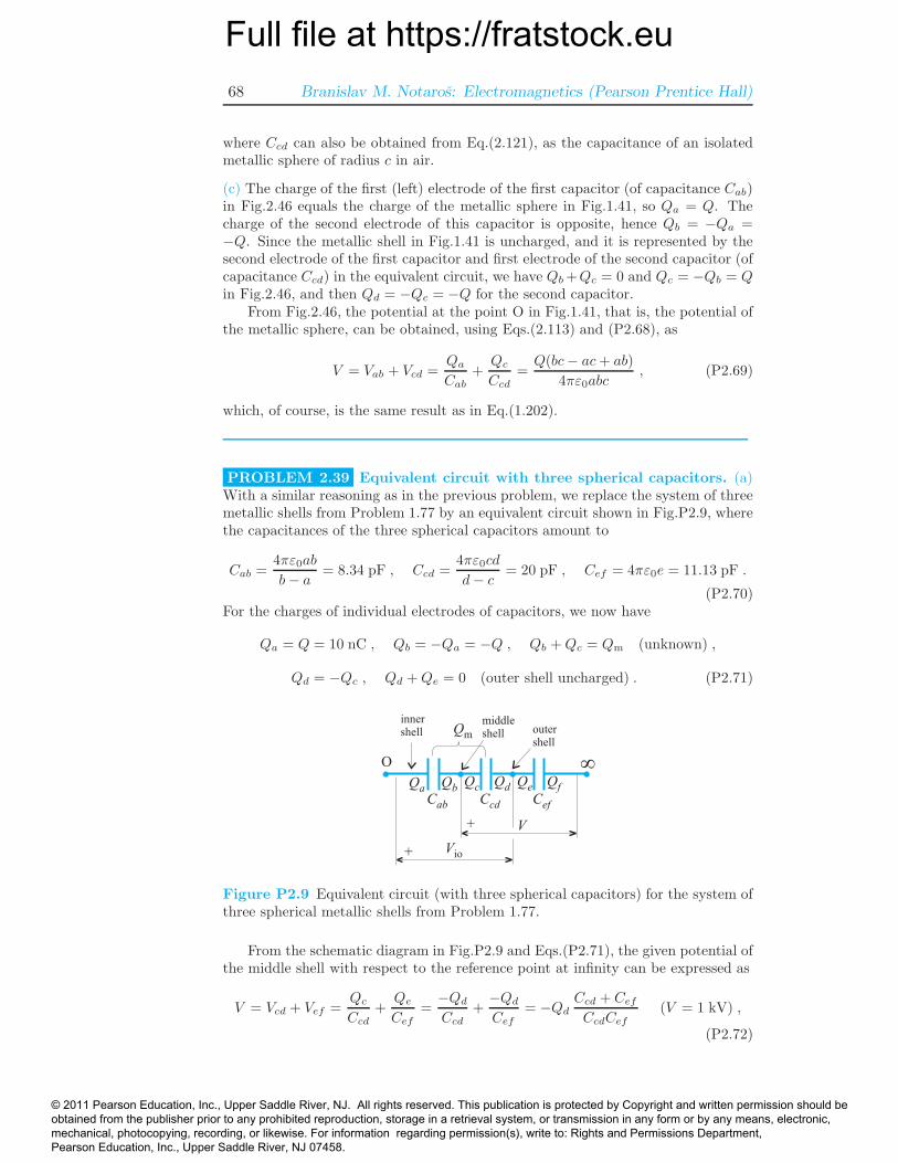
PROBLEM 2.39 Equivalent circuit with three spherical capacitors. (a)With a similar reasoning as in the previous problem, we replace the system of threemetallic shells from Problem 1.77 by an equivalent circuit shown in Fig.P2.9, wherethe capacitances of the three spherical capacitors amount to
Cab =4πε0ab
b− a = 8.34 pF , Ccd =4πε0cd
d− c = 20 pF , Cef = 4πε0e = 11.13 pF .
(P2.70)For the charges of individual electrodes of capacitors, we now have
Qa = Q = 10 nC , Qb = −Qa = −Q , Qb +Qc = Qm (unknown) ,
Qd = −Qc , Qd +Qe = 0 (outer shell uncharged) . (P2.71)
Vio
V+
+
O
Qa QbQc Qd
Cab Ccd
Qe Qf
Cef
innershell Qm
middleshell outer
shell
Figure P2.9 Equivalent circuit (with three spherical capacitors) for the system ofthree spherical metallic shells from Problem 1.77.
From the schematic diagram in Fig.P2.9 and Eqs.(P2.71), the given potential ofthe middle shell with respect to the reference point at infinity can be expressed as
V = Vcd + Vef =QcCcd
+QeCef
=−QdCcd
+−QdCef
= −QdCcd + CefCcdCef
(V = 1 kV) ,
(P2.72)
© 2011 Pearson Education, Inc., Upper Saddle River, NJ. All rights reserved. This publication is protected by Copyright and written permission should be obtained from the publisher prior to any prohibited reproduction, storage in a retrieval system, or transmission in any form or by any means, electronic, mechanical, photocopying, recording, or likewise. For information regarding permission(s), write to: Rights and Permissions Department, Pearson Education, Inc., Upper Saddle River, NJ 07458.
Full file at https://fratstock.euP2. Solutions to Problems: Dielectrics, Capacitance, Electric Energy 69
and hence, using Eqs.(P2.70) as well, the charge of the middle shell (Qm) turns outto be
Qd = − CcdCefV
Ccd + Cef= −7.15 nC −→ Qm = Qb +Qc = −Q−Qd = −2.85 nC .
(P2.73)The voltage between the inner and outer shells equals
Vio = Vab + Vcd =QaCab
+QcCcd
=Q
Cab+−QdCcd
= 1.55 kV , (P2.74)
the same as in Eq.(P1.154).
(b) For changed conditions in the circuit in Fig.P2.9 (and a slightly different nota-tion), set in Problem 1.78, the charges of capacitor electrodes are given by
Qa = Q1 = 2 nC , Qb = −Qa = −Q1 , Qb +Qc = Q2 = Qm (unknown) ,
Qd = −Qc , Qd +Qe = Q3 = −2 nC (outer shell is now charged) , (P2.75)
from which the charges of the second and third capacitors are Qc = Q1 + Q2 andQe = Q1 + Q2 + Q3, respectively. Since the voltage between the inner and outershells is zero, we obtain the charge of the middle shell (Q2) as follows:
0 = Vab + Vcd =QaCab
+QcCcd
=Q1
Cab+Q1 +Q2
Ccd−→ Q2 = −6.8 nC . (P2.76)
Finally, the potential of the inner and outer shells (V1 = V3) and that of the middleshell (V2), with respect to the reference point at infinity, are
V1 = V3 = Vef =QeCef
=Q1 +Q2 +Q3
Cef= −611 V ,
V2 = Vcd + V3 =QcCcd
+ V3 =(Q1 +Q2)
Ccd+ V3 = −851 V , (P2.77)
which are the same results as in Problem 1.78.
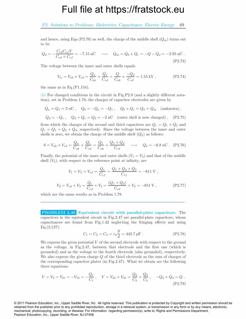
PROBLEM 2.40 Equivalent circuit with parallel-plate capacitors. Thecapacitors in the equivalent circuit in Fig.2.47 are parallel-plate capacitors, whosecapacitances are found from Fig.1.42 neglecting the fringing effects and usingEq.(2.127):
C1 = C2 = C3 = ε0S
d= 442.7 pF . (P2.78)
We express the given potential V of the second electrode with respect to the groundas the voltage, in Fig.2.47, between that electrode and the first one (which isgrounded) and as the voltage to the fourth electrode (also grounded), respectively.We also express the given charge Q of the third electrode as the sum of charges ofthe corresponding capacitor plates (in Fig.2.47). What we obtain are the followingthree equations:
V = V2 = V21 = −V12 = −Q1
C1, V = V23 + V34 =
Q2
C2+Q3
C3, −Q2 +Q3 = Q ,
(P2.79)
© 2011 Pearson Education, Inc., Upper Saddle River, NJ. All rights reserved. This publication is protected by Copyright and written permission should be obtained from the publisher prior to any prohibited reproduction, storage in a retrieval system, or transmission in any form or by any means, electronic, mechanical, photocopying, recording, or likewise. For information regarding permission(s), write to: Rights and Permissions Department, Pearson Education, Inc., Upper Saddle River, NJ 07458.
Full file at https://fratstock.eu70 Branislav M. Notaros: Electromagnetics (Pearson Prentice Hall)
whose solution is Q1 = −885.4 nC, Q2 = −557.3 nC, and Q3 = 1.443 µC. By meansof Eqs.(2.126) and (2.113), the electric field intensities in capacitors in Fig.2.47, i.e.,between the electrodes in Fig.1.42(b), amount to
E1 =V12
d=
Q1
C1d= −100 kV/m , E2 =
V23
d=
Q2
C2d= −63 kV/m ,
E3 =V34
d=
Q3
C3d= 163 kV/m . (P2.80)
Of course, E4 = 0 in Fig.1.42(b), as the field in the (fourth) capacitor with short-circuited plates, which is not shown in Fig.2.47.
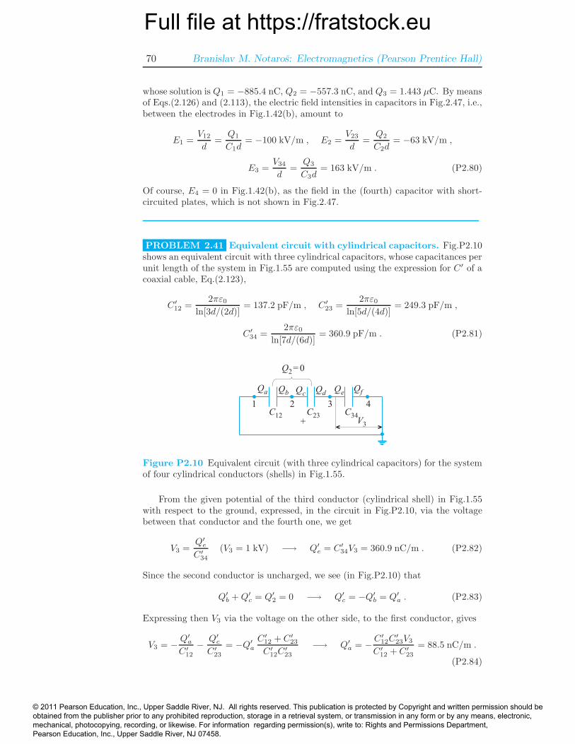
PROBLEM 2.41 Equivalent circuit with cylindrical capacitors. Fig.P2.10shows an equivalent circuit with three cylindrical capacitors, whose capacitances perunit length of the system in Fig.1.55 are computed using the expression for C′ of acoaxial cable, Eq.(2.123),
C′12 =
2πε0ln[3d/(2d)]
= 137.2 pF/m , C′23 =
2πε0ln[5d/(4d)]
= 249.3 pF/m ,
C′34 =
2πε0ln[7d/(6d)]
= 360.9 pF/m . (P2.81)
Qa Qb Qc QdQe
Qf
1 2 3 4C12 C23 C34
+ V3
Q2 = 0
Figure P2.10 Equivalent circuit (with three cylindrical capacitors) for the systemof four cylindrical conductors (shells) in Fig.1.55.
From the given potential of the third conductor (cylindrical shell) in Fig.1.55with respect to the ground, expressed, in the circuit in Fig.P2.10, via the voltagebetween that conductor and the fourth one, we get
V3 =Q′e
C′34
(V3 = 1 kV) −→ Q′e = C′
34V3 = 360.9 nC/m . (P2.82)
Since the second conductor is uncharged, we see (in Fig.P2.10) that
Q′b +Q′
c = Q′2 = 0 −→ Q′
c = −Q′b = Q′
a . (P2.83)
Expressing then V3 via the voltage on the other side, to the first conductor, gives
V3 = − Q′a
C′12
− Q′c
C′23
= −Q′a
C′12 + C′
23
C′12C
′23
−→ Q′a = −C
′12C
′23V3
C′12 + C′
23
= 88.5 nC/m .
(P2.84)
© 2011 Pearson Education, Inc., Upper Saddle River, NJ. All rights reserved. This publication is protected by Copyright and written permission should be obtained from the publisher prior to any prohibited reproduction, storage in a retrieval system, or transmission in any form or by any means, electronic, mechanical, photocopying, recording, or likewise. For information regarding permission(s), write to: Rights and Permissions Department, Pearson Education, Inc., Upper Saddle River, NJ 07458.
Full file at https://fratstock.euP2. Solutions to Problems: Dielectrics, Capacitance, Electric Energy 71
Hence, the total charges p.u.l. of the first and third conductors (in Fig.1.55) comeout [from Fig.P2.10 and Eqs.(P2.82)-(P2.84)] to be
Q′1 = Q′
a = −88.5 nC/m , Q′3 = Q′
d+Q′e = −Q′
c+Q′e = −Q′
a+Q′e = 450 nC/m ,
(P2.85)and the results are the same as those obtained in Problem 1.79.
Section 2.14 Analysis of Capacitors withInhomogeneous Dielectrics
PROBLEM 2.42 Spherical capacitor with a solid and liquid dielectric.In the first (old) electrostatic state, the charge of the capacitor is, from Eq.(2.164),
Q = 4πε0
(b− aεr1ab
+c− bεr2bc
)−1
V = 1.152 nC (V = Vsource = 100 V) . (P2.86)
Upon the voltage source is disconnected, and the capacitor is left to itself, thischarge remains the same in the new electrostatic state, in which the capacitanceof the capacitor is changed (oil is drained from the capacitor, so εr2 = 1), and thevoltage across open-circuited terminals of the capacitor turns out to be:
Vnew =Q
4πε0
(b− aεr1ab
+c− bbc
)
= 136.5 V . (P2.87)
PROBLEM 2.43 Oil drain without disconnecting the source. The capac-itor charge in the old electrostatic state is Q = 1.152 nC (previous problem), andthat in the new state (with εr2 = 1) amounts to
Qnew = 4πε0
(b− aεr1ab
+c− bbc
)−1
Vsource = 843.3 pC . (P2.88)
The difference equals the charge flow through the source circuit (in the directionfrom the positive end of the source toward the positive electrode of the capacitor,that with Q):
Qflow = ∆Q = Qnew −Q = −308.3 pC . (P2.89)
PROBLEM 2.44 Metallic sphere with dielectric coating. (a) This is aD-system, and the electric flux density vector, D, in both the dielectric coating andair is given by Eqs.(2.161) and (2.162), where Q is the charge of the metallic sphere.The electric field intensity vector is E1 = D/(εrε0) in the coating and E2 = D/ε0 inair. From this field, we can express, by integration, the potential of the sphere (withrespect to the reference point at infinity), V , in terms of Q, and find its capacitance(C) employing Eq.(2.116). Alternatively, we can consider the dielectrically coated
© 2011 Pearson Education, Inc., Upper Saddle River, NJ. All rights reserved. This publication is protected by Copyright and written permission should be obtained from the publisher prior to any prohibited reproduction, storage in a retrieval system, or transmission in any form or by any means, electronic, mechanical, photocopying, recording, or likewise. For information regarding permission(s), write to: Rights and Permissions Department, Pearson Education, Inc., Upper Saddle River, NJ 07458.
Full file at https://fratstock.eu72 Branislav M. Notaros: Electromagnetics (Pearson Prentice Hall)
metallic sphere in Fig.2.48 as a special case of the spherical capacitor with twodielectric layers in Fig.2.27, and specialize Eq.(2.164) specifying εr1 = εr, εr2 = 1,and c→∞, to obtain
C = 4πε0
(b− aεrab
+1
b
)−1
=4πεrε0ab
b− a+ εra= 2.224 pF . (P2.90)
(b) Using Eq.(2.58) or (1.191), the density of free surface charge on the metallicsphere in Fig.2.48 amounts to
ρs = D(a+) =Q
4πa2=
CV
4πa2= 1.77 µC/m2 . (P2.91)
(c) Eq.(2.60) tells us that there is no bound volume charge in a homogeneous linearmedium with no free volume charge; so, in both the dielectric coating and air inFig.2.48, ρp = 0.
(d) By means of Eqs.(2.61) and (P2.91), the bound surface charge density on thesurface of the dielectric coating next to the metallic sphere equals
ρpsa = −εr − 1
εrρs = −1.327 µC/m2 , (P2.92)
while, from Eqs.(2.23), (2.59), and (2.47), the bound surface charge density on theother surface of the coating is
ρpsb = P (b−) =εr − 1
εrD(b−) =
εr − 1
εr
CV
4πb2= 147.6 nC/m2 . (P2.93)
Q
e
e0
E
a
r
b
rpsa
rpsb
rs1
rs2
rs3
rs4
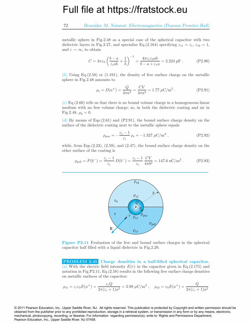
Figure P2.11 Evaluation of the free and bound surface charges in the sphericalcapacitor half filled with a liquid dielectric in Fig.2.29.
PROBLEM 2.45 Charge densities in a half-filled spherical capacitor.(a) With the electric field intensity E(r) in the capacitor given in Eq.(2.175) andnotation in Fig.P2.11, Eq.(2.58) results in the following free surface charge densitieson metallic surfaces of the capacitor:
ρs1 = εrε0E(a+) =εrQ
2π(εr + 1)a2= 2.98 µC/m2 , ρs2 = ε0E(a+) =
Q
2π(εr + 1)a2
© 2011 Pearson Education, Inc., Upper Saddle River, NJ. All rights reserved. This publication is protected by Copyright and written permission should be obtained from the publisher prior to any prohibited reproduction, storage in a retrieval system, or transmission in any form or by any means, electronic, mechanical, photocopying, recording, or likewise. For information regarding permission(s), write to: Rights and Permissions Department, Pearson Education, Inc., Upper Saddle River, NJ 07458.
Full file at https://fratstock.euP2. Solutions to Problems: Dielectrics, Capacitance, Electric Energy 73
= 995 nC/m2 , ρs3 = −εrε0E(b−) = − εrQ
2π(εr + 1)b2= −119 nC/m2 ,
ρs4 = −ε0E(b−) = − Q
2π(εr + 1)b2= −39.8 nC/m2 . (P2.94)
(b) From Eq.(2.61) and (P2.94), bound surface charge densities on dielectric surfacesnext to capacitor electrodes in Fig.P2.11 are
ρpsa = −εr − 1
εrρs1 = −1.99 µC/m2 , ρpsb = −εr − 1
εrρs3 = 79.6 nC/m2 ,
(P2.95)while Eq.(2.23) tells us that there is no bound charge on the surfaces dielectric-airin the capacitor, as vectors E and P are tangential on these surfaces.
PROBLEM 2.46 Empty and half-filled spherical capacitor. UsingEq.(2.119), the charge of the empty (air-filled) spherical capacitor in the first elec-trostatic state equals
Q = CV =4πε0abV
b− a (V = Vsource = 15 kV) . (P2.96)
Eq.(2.176) then gives the following for the voltage across the open-circuited termi-nals of the capacitor, half filled with a liquid dielectric, in the new state (Q is thesame):
Vnew =Q
Cnew=
(b− a)Q2π(εr + 1)ε0ab
=2V
εr + 1= 8.571 kV . (P2.97)
PROBLEM 2.47 Metallic sphere half embedded in a dielectric. (a) Thisis anE-system, and the electric field intensity vector (E) is entirely radial. Moreover,it can be evaluated in the same way as in Fig.2.29 and Eq.(2.174), and is given inEq.(2.175). By integrating E(r) from the metallic sphere surface to the referencepoint at infinity, we can obtain the potential of the sphere and its capacitance.Alternatively, we can use Eq.(2.176) with b→∞. In either way, the capacitance ofthe metallic sphere in Fig.2.49 comes out to be
C = 2π(εr + 1)ε0a . (P2.98)
(b) The two terms in the application of the generalized Gauss’ law in Eq.(2.174)actually show how the charge Q of the metallic sphere in Fig.2.49 is distributedbetween its two halves; the ratio of the charge on the lower half, Q1,to the chargeof the upper half, Q2, is thus
Q1
Q2=D1
D2=εrε0E
ε0E= εr , (P2.99)
and hence the portion of Q that is located on the upper half of the sphere amountsto
Q2
Q=
1
εr + 1. (P2.100)
© 2011 Pearson Education, Inc., Upper Saddle River, NJ. All rights reserved. This publication is protected by Copyright and written permission should be obtained from the publisher prior to any prohibited reproduction, storage in a retrieval system, or transmission in any form or by any means, electronic, mechanical, photocopying, recording, or likewise. For information regarding permission(s), write to: Rights and Permissions Department, Pearson Education, Inc., Upper Saddle River, NJ 07458.
Full file at https://fratstock.eu74 Branislav M. Notaros: Electromagnetics (Pearson Prentice Hall)
PROBLEM 2.48 Coaxial cable with two coaxial dielectric layers. Thisis a cylindrical version of the structure in Fig.2.27, so Eq.(2.162) becomes
D(r) =Q′
2πr, a < r < c , (P2.101)
and the voltage between the conductors of the coaxial cable in Fig.2.50 is
V =
∫ b
r=a
D(r)
ε1dr +
∫ c
r=b
D(r)
ε2dr =
Q′
2π
(1
ε1lnb
a+
1
ε2lnc
b
)
. (P2.102)
Hence, the capacitance per unit length of the cable amounts to
C′ =Q′
V= 2πε0
(1
εr1lnb
a+
1
εr2lnc
b
)−1
= 114.7 pF/m . (P2.103)
Alternatively, we can find C′ of the cable in Fig.2.50 as the equivalent totalp.u.l. capacitance of a series connection, Eq.(2.156), of two coaxial cables withhomogeneous dielectrics, whose p.u.l. capacitances, from Eq.(2.123), are given by
C′1 =
2πεr1ε0ln(b/a)
and C′2 =
2πεr2ε0ln(c/b)
. (P2.104)
PROBLEM 2.49 Coaxial cable with a radial variation of permittivity.(a) This, again, is a cylindrical version of the structure analyzed in Example 2.19.The electric flux density vector in the dielectric is radial with respect to the cableaxis and its magnitude is given by D(r) = Q′/(2πr). Similarly to the integration inEq.(2.169), the voltage of the cable can be computed as
V =
∫ b
a
E(r) dr =
∫ b
a
D(r)
εr(r)ε0dr =
Q′
2πε0
∫ b
a
dr
rεr(r), (P2.105)
and its per-unit-length capacitance as
C′ =Q′
V= 2πε0
[∫ b
a
dr
rεr(r)
]−1
=2πε0b
b− a = 69.54 pF/m . (P2.106)
(b) The volume and surface bound charge densities in the dielectric are found asin Eqs.(2.170)-(2.172) [of course, here we use the formula for the divergence incylindrical coordinates, Eq.(1.170), to compute ρp]:
P (r) =εr(r)− 1
εr(r)D(r) =
εr(r)− 1
εr(r)
C′V
2πr=ε0bV
b− a
(1
r− a
r2
)
−→ ρp = −∇ ·P = −1
r
d
dr[rP (r)] = − ε0abV
(b− a)r3 = −5ε0aV
4r3,
ρpsa = −P (a+) = 0 , ρpsb = P (b−) =ε0V
5a. (P2.107)
© 2011 Pearson Education, Inc., Upper Saddle River, NJ. All rights reserved. This publication is protected by Copyright and written permission should be obtained from the publisher prior to any prohibited reproduction, storage in a retrieval system, or transmission in any form or by any means, electronic, mechanical, photocopying, recording, or likewise. For information regarding permission(s), write to: Rights and Permissions Department, Pearson Education, Inc., Upper Saddle River, NJ 07458.
Full file at https://fratstock.euP2. Solutions to Problems: Dielectrics, Capacitance, Electric Energy 75
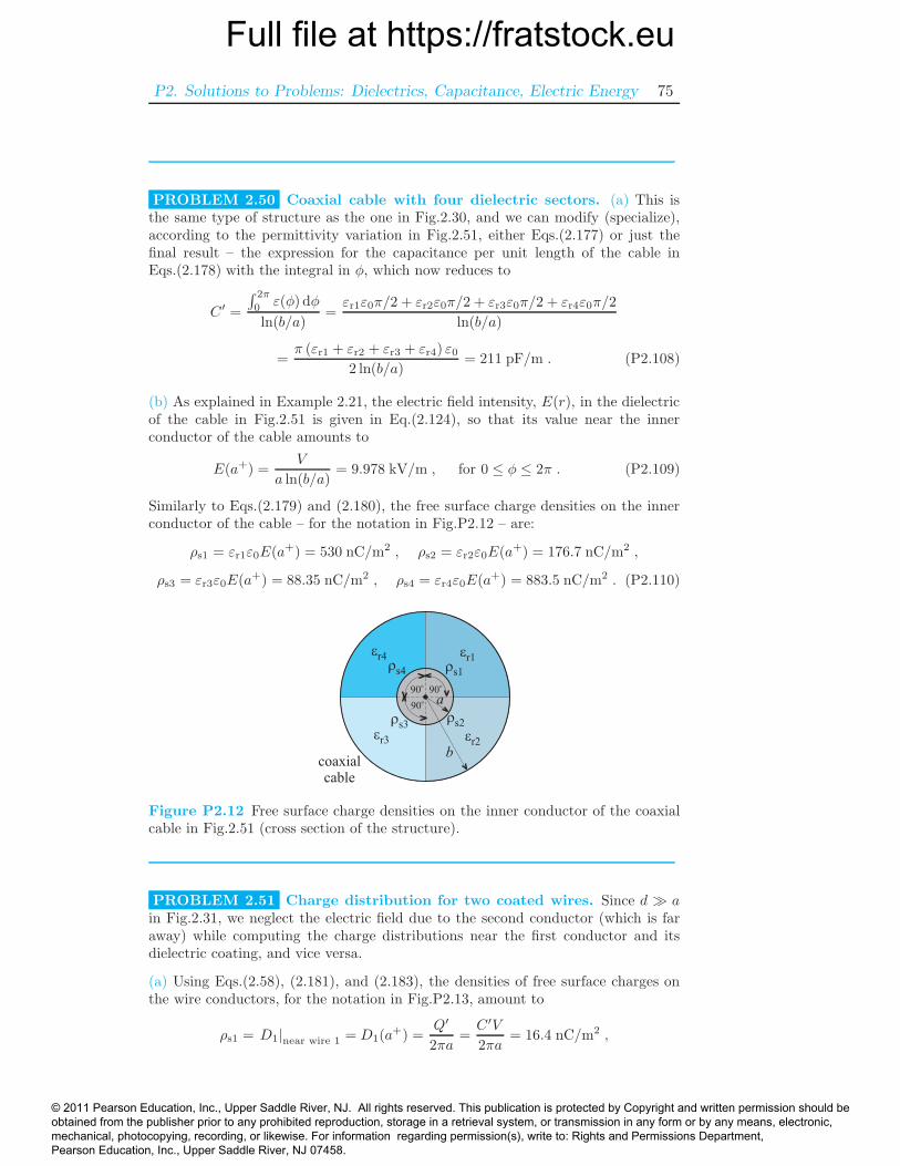
PROBLEM 2.50 Coaxial cable with four dielectric sectors. (a) This isthe same type of structure as the one in Fig.2.30, and we can modify (specialize),according to the permittivity variation in Fig.2.51, either Eqs.(2.177) or just thefinal result – the expression for the capacitance per unit length of the cable inEqs.(2.178) with the integral in φ, which now reduces to
C′ =
∫ 2π
0 ε(φ) dφ
ln(b/a)=εr1ε0π/2 + εr2ε0π/2 + εr3ε0π/2 + εr4ε0π/2
ln(b/a)
=π (εr1 + εr2 + εr3 + εr4) ε0
2 ln(b/a)= 211 pF/m . (P2.108)
(b) As explained in Example 2.21, the electric field intensity, E(r), in the dielectricof the cable in Fig.2.51 is given in Eq.(2.124), so that its value near the innerconductor of the cable amounts to
E(a+) =V
a ln(b/a)= 9.978 kV/m , for 0 ≤ φ ≤ 2π . (P2.109)
Similarly to Eqs.(2.179) and (2.180), the free surface charge densities on the innerconductor of the cable – for the notation in Fig.P2.12 – are:
ρs1 = εr1ε0E(a+) = 530 nC/m2 , ρs2 = εr2ε0E(a+) = 176.7 nC/m2 ,
ρs3 = εr3ε0E(a+) = 88.35 nC/m2 , ρs4 = εr4ε0E(a+) = 883.5 nC/m2 . (P2.110)
er3 er2
er4 er1
90o
90o
90o
a
bcoaxialcable
rs1
rs2rs3
rs4
Figure P2.12 Free surface charge densities on the inner conductor of the coaxialcable in Fig.2.51 (cross section of the structure).
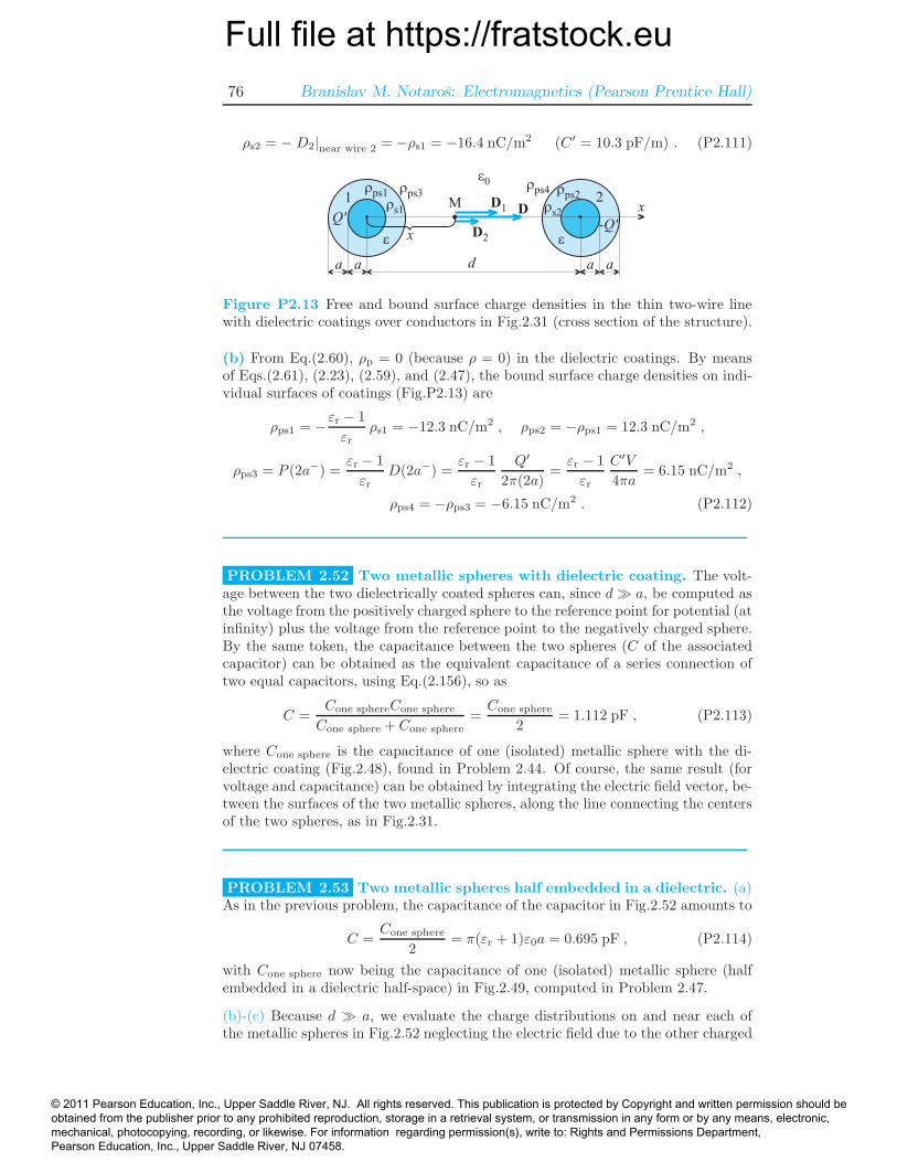
PROBLEM 2.51 Charge distribution for two coated wires. Since d ≫ ain Fig.2.31, we neglect the electric field due to the second conductor (which is faraway) while computing the charge distributions near the first conductor and itsdielectric coating, and vice versa.
(a) Using Eqs.(2.58), (2.181), and (2.183), the densities of free surface charges onthe wire conductors, for the notation in Fig.P2.13, amount to
ρs1 = D1|near wire 1 = D1(a+) =
Q′
2πa=C′V
2πa= 16.4 nC/m2 ,
© 2011 Pearson Education, Inc., Upper Saddle River, NJ. All rights reserved. This publication is protected by Copyright and written permission should be obtained from the publisher prior to any prohibited reproduction, storage in a retrieval system, or transmission in any form or by any means, electronic, mechanical, photocopying, recording, or likewise. For information regarding permission(s), write to: Rights and Permissions Department, Pearson Education, Inc., Upper Saddle River, NJ 07458.
Full file at https://fratstock.eu76 Branislav M. Notaros: Electromagnetics (Pearson Prentice Hall)
ρs2 = − D2|near wire 2 = −ρs1 = −16.4 nC/m2 (C′ = 10.3 pF/m) . (P2.111)
e e
da a aa
1 2
x
D1 D
D2
xMQ'
-Q'
e0
rs1 rs2
rps1 rps2rps3
rps4
Figure P2.13 Free and bound surface charge densities in the thin two-wire linewith dielectric coatings over conductors in Fig.2.31 (cross section of the structure).
(b) From Eq.(2.60), ρp = 0 (because ρ = 0) in the dielectric coatings. By meansof Eqs.(2.61), (2.23), (2.59), and (2.47), the bound surface charge densities on indi-vidual surfaces of coatings (Fig.P2.13) are
ρps1 = −εr − 1
εrρs1 = −12.3 nC/m2 , ρps2 = −ρps1 = 12.3 nC/m2 ,
ρps3 = P (2a−) =εr − 1
εrD(2a−) =
εr − 1
εr
Q′
2π(2a)=εr − 1
εr
C′V
4πa= 6.15 nC/m2 ,
ρps4 = −ρps3 = −6.15 nC/m2 . (P2.112)
PROBLEM 2.52 Two metallic spheres with dielectric coating. The volt-age between the two dielectrically coated spheres can, since d≫ a, be computed asthe voltage from the positively charged sphere to the reference point for potential (atinfinity) plus the voltage from the reference point to the negatively charged sphere.By the same token, the capacitance between the two spheres (C of the associatedcapacitor) can be obtained as the equivalent capacitance of a series connection oftwo equal capacitors, using Eq.(2.156), so as
C =Cone sphereCone sphere
Cone sphere + Cone sphere=Cone sphere
2= 1.112 pF , (P2.113)
where Cone sphere is the capacitance of one (isolated) metallic sphere with the di-electric coating (Fig.2.48), found in Problem 2.44. Of course, the same result (forvoltage and capacitance) can be obtained by integrating the electric field vector, be-tween the surfaces of the two metallic spheres, along the line connecting the centersof the two spheres, as in Fig.2.31.
PROBLEM 2.53 Two metallic spheres half embedded in a dielectric. (a)As in the previous problem, the capacitance of the capacitor in Fig.2.52 amounts to
C =Cone sphere
2= π(εr + 1)ε0a = 0.695 pF , (P2.114)
with Cone sphere now being the capacitance of one (isolated) metallic sphere (halfembedded in a dielectric half-space) in Fig.2.49, computed in Problem 2.47.
(b)-(c) Because d ≫ a, we evaluate the charge distributions on and near each ofthe metallic spheres in Fig.2.52 neglecting the electric field due to the other charged
© 2011 Pearson Education, Inc., Upper Saddle River, NJ. All rights reserved. This publication is protected by Copyright and written permission should be obtained from the publisher prior to any prohibited reproduction, storage in a retrieval system, or transmission in any form or by any means, electronic, mechanical, photocopying, recording, or likewise. For information regarding permission(s), write to: Rights and Permissions Department, Pearson Education, Inc., Upper Saddle River, NJ 07458.
Full file at https://fratstock.euP2. Solutions to Problems: Dielectrics, Capacitance, Electric Energy 77
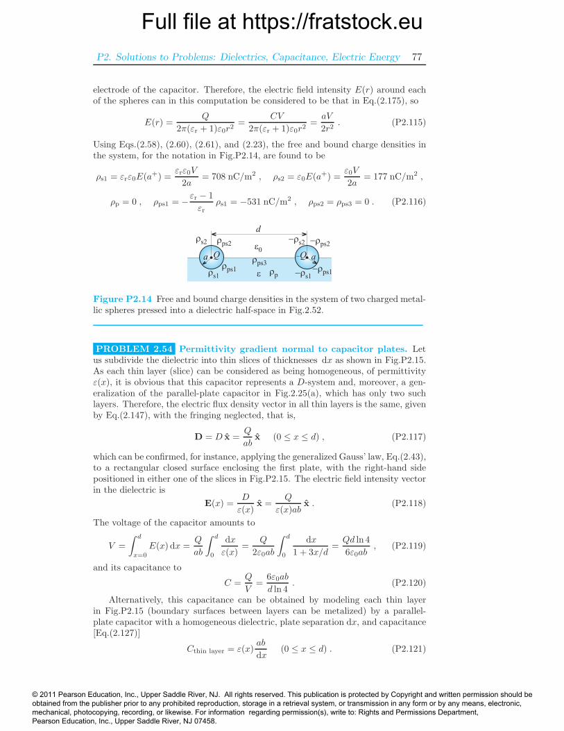
electrode of the capacitor. Therefore, the electric field intensity E(r) around eachof the spheres can in this computation be considered to be that in Eq.(2.175), so
E(r) =Q
2π(εr + 1)ε0r2=
CV
2π(εr + 1)ε0r2=aV
2r2. (P2.115)
Using Eqs.(2.58), (2.60), (2.61), and (2.23), the free and bound charge densities inthe system, for the notation in Fig.P2.14, are found to be
ρs1 = εrε0E(a+) =εrε0V
2a= 708 nC/m2 , ρs2 = ε0E(a+) =
ε0V
2a= 177 nC/m2 ,
ρp = 0 , ρps1 = −εr − 1
εrρs1 = −531 nC/m2 , ρps2 = ρps3 = 0 . (P2.116)
e0
e
d
a aQ -Q
rs1
rs2
rps1
rps2
rps3
-rs1
-rs2
-rps1
-rps2
rp
Figure P2.14 Free and bound charge densities in the system of two charged metal-lic spheres pressed into a dielectric half-space in Fig.2.52.
PROBLEM 2.54 Permittivity gradient normal to capacitor plates. Letus subdivide the dielectric into thin slices of thicknesses dx as shown in Fig.P2.15.As each thin layer (slice) can be considered as being homogeneous, of permittivityε(x), it is obvious that this capacitor represents a D-system and, moreover, a gen-eralization of the parallel-plate capacitor in Fig.2.25(a), which has only two suchlayers. Therefore, the electric flux density vector in all thin layers is the same, givenby Eq.(2.147), with the fringing neglected, that is,
D = D x =Q
abx (0 ≤ x ≤ d) , (P2.117)
which can be confirmed, for instance, applying the generalized Gauss’ law, Eq.(2.43),to a rectangular closed surface enclosing the first plate, with the right-hand sidepositioned in either one of the slices in Fig.P2.15. The electric field intensity vectorin the dielectric is
E(x) =D
ε(x)x =
Q
ε(x)abx . (P2.118)
The voltage of the capacitor amounts to
V =
∫ d
x=0
E(x) dx =Q
ab
∫ d
0
dx
ε(x)=
Q
2ε0ab
∫ d
0
dx
1 + 3x/d=Qd ln 4
6ε0ab, (P2.119)
and its capacitance to
C =Q
V=
6ε0ab
d ln 4. (P2.120)
Alternatively, this capacitance can be obtained by modeling each thin layerin Fig.P2.15 (boundary surfaces between layers can be metalized) by a parallel-plate capacitor with a homogeneous dielectric, plate separation dx, and capacitance[Eq.(2.127)]
Cthin layer = ε(x)ab
dx(0 ≤ x ≤ d) . (P2.121)
© 2011 Pearson Education, Inc., Upper Saddle River, NJ. All rights reserved. This publication is protected by Copyright and written permission should be obtained from the publisher prior to any prohibited reproduction, storage in a retrieval system, or transmission in any form or by any means, electronic, mechanical, photocopying, recording, or likewise. For information regarding permission(s), write to: Rights and Permissions Department, Pearson Education, Inc., Upper Saddle River, NJ 07458.
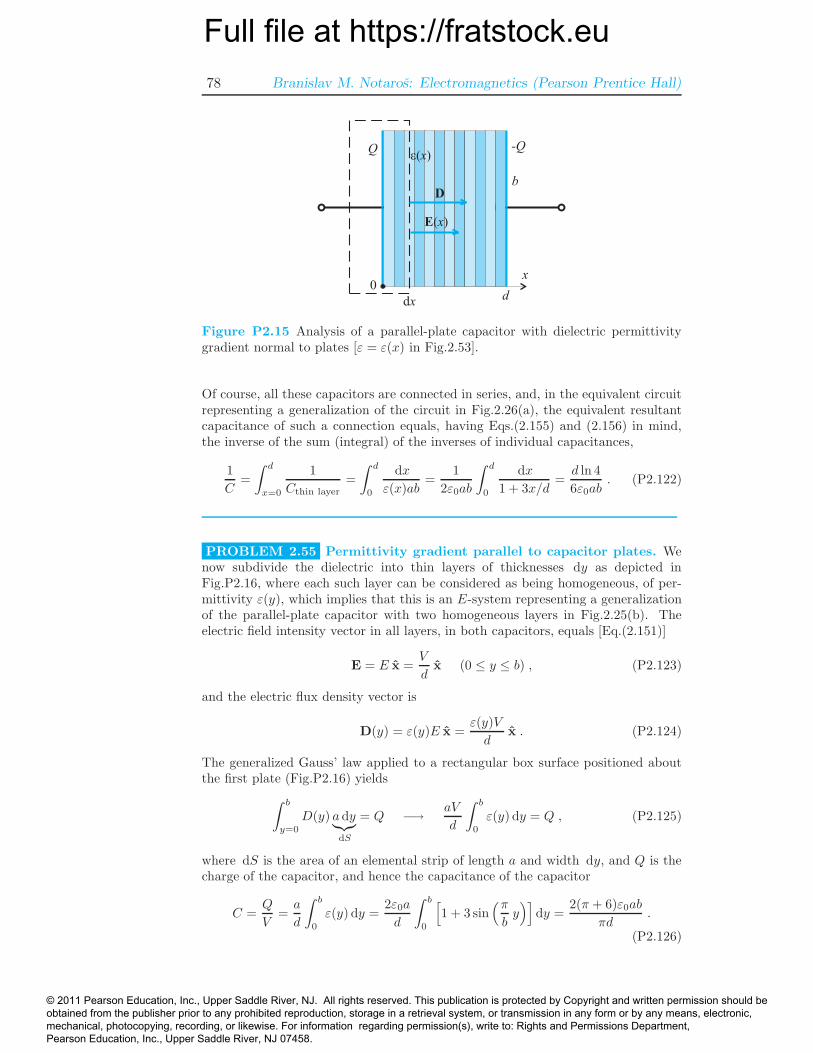
Full file at https://fratstock.eu78 Branislav M. Notaros: Electromagnetics (Pearson Prentice Hall)
x
b
d0
Q -Qe(x)
dx
E( )x
D
Figure P2.15 Analysis of a parallel-plate capacitor with dielectric permittivitygradient normal to plates [ε = ε(x) in Fig.2.53].
Of course, all these capacitors are connected in series, and, in the equivalent circuitrepresenting a generalization of the circuit in Fig.2.26(a), the equivalent resultantcapacitance of such a connection equals, having Eqs.(2.155) and (2.156) in mind,the inverse of the sum (integral) of the inverses of individual capacitances,
1
C=
∫ d
x=0
1
Cthin layer=
∫ d
0
dx
ε(x)ab=
1
2ε0ab
∫ d
0
dx
1 + 3x/d=d ln 4
6ε0ab. (P2.122)
PROBLEM 2.55 Permittivity gradient parallel to capacitor plates. Wenow subdivide the dielectric into thin layers of thicknesses dy as depicted inFig.P2.16, where each such layer can be considered as being homogeneous, of per-mittivity ε(y), which implies that this is an E-system representing a generalizationof the parallel-plate capacitor with two homogeneous layers in Fig.2.25(b). Theelectric field intensity vector in all layers, in both capacitors, equals [Eq.(2.151)]
E = E x =V
dx (0 ≤ y ≤ b) , (P2.123)
and the electric flux density vector is
D(y) = ε(y)E x =ε(y)V
dx . (P2.124)
The generalized Gauss’ law applied to a rectangular box surface positioned aboutthe first plate (Fig.P2.16) yields
∫ b
y=0
D(y) a dy︸︷︷︸
dS
= Q −→ aV
d
∫ b
0
ε(y) dy = Q , (P2.125)
where dS is the area of an elemental strip of length a and width dy, and Q is thecharge of the capacitor, and hence the capacitance of the capacitor
C =Q
V=a
d
∫ b
0
ε(y) dy =2ε0a
d
∫ b
0
[
1 + 3 sin(π
by)]
dy =2(π + 6)ε0ab
πd.
(P2.126)
© 2011 Pearson Education, Inc., Upper Saddle River, NJ. All rights reserved. This publication is protected by Copyright and written permission should be obtained from the publisher prior to any prohibited reproduction, storage in a retrieval system, or transmission in any form or by any means, electronic, mechanical, photocopying, recording, or likewise. For information regarding permission(s), write to: Rights and Permissions Department, Pearson Education, Inc., Upper Saddle River, NJ 07458.
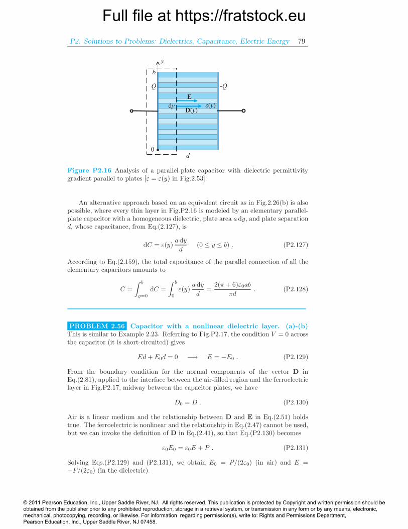
Full file at https://fratstock.euP2. Solutions to Problems: Dielectrics, Capacitance, Electric Energy 79
d
Q -Q
b
D( )y
E
y
0
dy e(y)
Figure P2.16 Analysis of a parallel-plate capacitor with dielectric permittivitygradient parallel to plates [ε = ε(y) in Fig.2.53].
An alternative approach based on an equivalent circuit as in Fig.2.26(b) is alsopossible, where every thin layer in Fig.P2.16 is modeled by an elementary parallel-plate capacitor with a homogeneous dielectric, plate area a dy, and plate separationd, whose capacitance, from Eq.(2.127), is
dC = ε(y)a dy
d(0 ≤ y ≤ b) . (P2.127)
According to Eq.(2.159), the total capacitance of the parallel connection of all theelementary capacitors amounts to
C =
∫ b
y=0
dC =
∫ b
0
ε(y)a dy
d=
2(π + 6)ε0ab
πd. (P2.128)
PROBLEM 2.56 Capacitor with a nonlinear dielectric layer. (a)-(b)This is similar to Example 2.23. Referring to Fig.P2.17, the condition V = 0 acrossthe capacitor (it is short-circuited) gives
Ed+ E0d = 0 −→ E = −E0 . (P2.129)
From the boundary condition for the normal components of the vector D inEq.(2.81), applied to the interface between the air-filled region and the ferroelectriclayer in Fig.P2.17, midway between the capacitor plates, we have
D0 = D . (P2.130)
Air is a linear medium and the relationship between D and E in Eq.(2.51) holdstrue. The ferroelectric is nonlinear and the relationship in Eq.(2.47) cannot be used,but we can invoke the definition of D in Eq.(2.41), so that Eq.(P2.130) becomes
ε0E0 = ε0E + P . (P2.131)
Solving Eqs.(P2.129) and (P2.131), we obtain E0 = P/(2ε0) (in air) and E =−P/(2ε0) (in the dielectric).
© 2011 Pearson Education, Inc., Upper Saddle River, NJ. All rights reserved. This publication is protected by Copyright and written permission should be obtained from the publisher prior to any prohibited reproduction, storage in a retrieval system, or transmission in any form or by any means, electronic, mechanical, photocopying, recording, or likewise. For information regarding permission(s), write to: Rights and Permissions Department, Pearson Education, Inc., Upper Saddle River, NJ 07458.
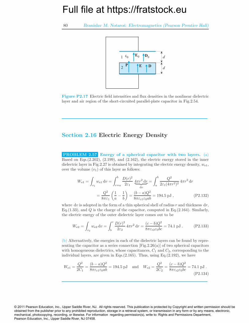
Full file at https://fratstock.eu80 Branislav M. Notaros: Electromagnetics (Pearson Prentice Hall)
e0 d
dP E
1
2
D0E0
D
Figure P2.17 Electric field intensities and flux densities in the nonlinear dielectriclayer and air region of the short-circuited parallel-plate capacitor in Fig.2.54.
Section 2.16 Electric Energy Density
PROBLEM 2.57 Energy of a spherical capacitor with two layers. (a)Based on Eqs.(2.202), (2.199), and (2.162), the electric energy stored in the innerdielectric layer in Fig.2.27 is obtained by integrating the electric energy density, we1,over the volume (v1) of this layer as follows:
We1 =
∫
v1
we1 dv =
∫ b
r=a
D(r)2
2ε14πr2 dr︸ ︷︷ ︸
dv
=
∫ b
a
Q2
2ε1(4πr2)24πr2 dr
=Q2
8πε1
(1
a− 1
b
)
=(b− a)Q2
8πεr1ε0ab= 194.5 pJ , (P2.132)
where dv is adopted in the form of a thin spherical shell of radius r and thickness dr,Eq.(1.33), and Q is the charge of the capacitor, computed in Eq.(2.164). Similarly,the electric energy of the outer dielectric layer comes out to be
We2 =
∫
v2
we2 dv =
∫ c
b
D(r)2
2ε24πr2 dr =
(c− b)Q2
8πεr2ε0bc= 74.1 pJ . (P2.133)
(b) Alternatively, the energies in each of the dielectric layers can be found by repre-senting the capacitor as a series connection [Fig.2.26(a)] of two spherical capacitorswith homogeneous dielectrics, whose capacitances, C1 and C2, corresponding to theindividual layers, are given in Eqs.(2.165). Thus, using Eq.(2.192), we have
We1 =Q2
2C1=
(b − a)Q2
8πεr1ε0ab= 194.5 pJ and We2 =
Q2
2C2=
(c− b)Q2
8πεr2ε0bc= 74.1 pJ .
(P2.134)
© 2011 Pearson Education, Inc., Upper Saddle River, NJ. All rights reserved. This publication is protected by Copyright and written permission should be obtained from the publisher prior to any prohibited reproduction, storage in a retrieval system, or transmission in any form or by any means, electronic, mechanical, photocopying, recording, or likewise. For information regarding permission(s), write to: Rights and Permissions Department, Pearson Education, Inc., Upper Saddle River, NJ 07458.
Full file at https://fratstock.euP2. Solutions to Problems: Dielectrics, Capacitance, Electric Energy 81
PROBLEM 2.58 Change in energy of a spherical capacitor. With theuse of Eq.(2.192), the change in electric energy of the capacitor between the twoelectrostatic states turns out to be
∆We = (We)new− (We)old =1
2QVnew−
1
2QVsource =
1
2Q (Vnew − Vsource) = 21 nJ ,
(P2.135)where Q = 1.152 nC, Vnew = 136.5 V, and Vsource = 100 V (Problem 2.42).
PROBLEM 2.59 Energy of a coated metallic sphere. We can metalize theequipotential surface r = b in the structure in Fig.2.48 and thus obtain two sphericalcapacitors, with electrode radii of the second (air-filled) one being b and c → ∞.Based on Eq.(2.192), the electric energies stored in the dielectric coating and in airin Fig.2.48 can then, respectively, be expressed as
We1 =Q2
2C1and We2 =
Q2
2C2, (P2.136)
where the charges of the two capacitors in the equivalent circuit in Fig.2.26(a)are the same, Q, and their capacitances are obtained from Eqs.(2.165) specifyingεr1 = εr, εr2 = 1, and c→∞:
C1 =4πεrε0ab
b − a and C2 = 4πε0b . (P2.137)
The required equality of two energies in Eqs.(P2.136), i.e., the requirement that 1/2of the total energy of the system is stored in the coating, implies the equality of thecapacitances in Eqs(P2.137), which further leads to
We1 = We2 −→ C1 = C2 −→ εra
b− a = 1 −→ b = (εr + 1) a = 5 cm .
(P2.138)
PROBLEM 2.60 Energy of a coaxial cable with two coaxial layers. Thisis a cylindrical version of the energy computation in Problem 2.57.
(a) Having in mind Eqs.(2.206) and (2.207) and the expression for the electric fluxdensity in the cable dielectric, D(r) = Q′/(2πr), we compute the electric energystored in the inner dielectric layer in Fig.2.50 per unit length of the coaxial cable byintegrating the electric energy density over the cross-sectional areas of the individuallayers, S1 and S2, which results in
W ′e1 =
∫
S1
we1 dS =
∫ b
r=a
D(r)2
2ε12πr dr︸ ︷︷ ︸
dS
=
∫ b
a
Q′2
2ε1(2πr)22πr dr =
Q′2
4πεr1ε0lnb
a
= 164 nJ/m , W ′e2 =
∫
S2
we2 dS =
∫ c
b
D(r)2
2ε22πr dr =
Q′2
4πεr2ε0lnc
b= 409 nJ/m ,
(P2.139)where dS is the area of an elementary ring (adopted for integration) of radius r andwidth dr, Eq.(1.60), Q′ = C′V , and C′ = 114.7 pF/m is the capacitance per unitlength of the cable, found in Problem 2.48.
(b) In the alternative approach, we represent the cable by the equivalent circuitin Fig.2.26(a) and use the p.u.l. capacitances C′
1 = 2πεr1ε0/ ln(b/a) and C′2 =
© 2011 Pearson Education, Inc., Upper Saddle River, NJ. All rights reserved. This publication is protected by Copyright and written permission should be obtained from the publisher prior to any prohibited reproduction, storage in a retrieval system, or transmission in any form or by any means, electronic, mechanical, photocopying, recording, or likewise. For information regarding permission(s), write to: Rights and Permissions Department, Pearson Education, Inc., Upper Saddle River, NJ 07458.
Full file at https://fratstock.eu82 Branislav M. Notaros: Electromagnetics (Pearson Prentice Hall)
2πεr2ε0/ ln(c/b) (Problem 2.48), to obtain [see also Eq.(2.208)]
W ′e1 =
Q′2
2C′1
=Q′2
4πεr1ε0lnb
a= 164 nJ/m , W ′
e2 =Q′2
2C′2
=Q′2
4πεr2ε0lnc
b= 409 nJ/m .
(P2.140)
PROBLEM 2.61 Energy of a half-filled spherical capacitor. This is aspherical version of the energy computation in Example 2.26. With the electricfield intensity E(r) in the capacitor in Fig.2.29 given in Eq.(2.175), the electricenergy contained in the liquid, i.e., in the lower half of the space between electrodes(volume v1), is computed as
We1 =
∫
v1
we1 dv =
∫ b
r=a
1
2εrε0E(r)2
︸ ︷︷ ︸
we1
2πr2 dr︸ ︷︷ ︸
dv
=
∫ b
a
1
2εrε0
Q2
[2π(εr + 1)ε0r2]22πr2 dr
=εr(b − a)Q2
4π(εr + 1)2ε0ab, (P2.141)
where dv is the volume of a thin hemispherical shell of radius r and thickness dr[1/2 of dv in Eq.(1.33)].
PROBLEM 2.62 Energy of a coaxial cable with four sectors. Like thecoaxial cable in Fig.2.33, this is an E-system, and the electric field (E) is the sameas in the air-filled coaxial cable, Eq.(2.124). Similarly to the energy computation inEq.(2.210), the per-unit-length electric energy contained in the 90◦ dielectric sectorof relative permittivity εr1 (εr1 = 6) in Fig.2.51 is found to be
E(r) =V
r ln(b/a)−→ W ′
e1 =
∫ b
r=a
1
2ε1E(r)2
︸ ︷︷ ︸
we1
π
2r dr
︸ ︷︷ ︸
dS1
=πεr1ε0V
2
4 ln2(b/a)
∫ b
a
dr
r
=πεr1ε0V
2
4 ln(b/a)= 20.82 nJ/m , (P2.142)
with dS1 standing for the surface area of a quarter (determined by the angle π/2)of a thin ring of radius r and width dr [ dS1 is 1/4 of dS in Eq.(1.60)]. In the sameway, the p.u.l. energies in the remaining three 90◦ dielectric sectors in Fig.2.51 are
W ′e2 =
πεr2ε0V2
4 ln(b/a)= 6.94 nJ/m , W ′
e3 =πεr3ε0V
2
4 ln(b/a)= 3.47 nJ/m ,
W ′e4 =
πεr4ε0V2
4 ln(b/a)= 34.7 nJ/m . (P2.143)
PROBLEM 2.63 Energy of a capacitor with a variable permittivity.Based on Eqs.(2.202) and (2.199) and the fact that D = const in the capacitor
© 2011 Pearson Education, Inc., Upper Saddle River, NJ. All rights reserved. This publication is protected by Copyright and written permission should be obtained from the publisher prior to any prohibited reproduction, storage in a retrieval system, or transmission in any form or by any means, electronic, mechanical, photocopying, recording, or likewise. For information regarding permission(s), write to: Rights and Permissions Department, Pearson Education, Inc., Upper Saddle River, NJ 07458.
Full file at https://fratstock.euP2. Solutions to Problems: Dielectrics, Capacitance, Electric Energy 83
dielectric (Problem 2.54), the total electric energy of the capacitor (We) can becomputed as
We =
∫
v
we dv =
∫ d
x=0
D2
2ε(x)ab dx︸ ︷︷ ︸
dv
=abD2
2
∫ d
0
dx
ε(x)=abD2
4ε0
∫ d
0
dx
1 + 3x/d,
(P2.144)where dv is adopted in the form of a thin flat layer (slice) of thickness dx. Bythe same token, the energy contained in the first half (from x = 0 to x = d/2) ofthe dielectric, We1, can be obtained by replacing the upper limit (d) in the aboveintegrals by d/2. Hence, the percentage of We contained in the first half of thedielectric turns out to be
We1
We=
∫ d/2
0dx
1+3x/d∫ d
0dx
1+3x/d
=ln(5/2)
ln 4= 66.1% . (P2.145)
PROBLEM 2.64 Energy of a capacitor with an inhomogeneous dielec-tric. Given that now E = const in the dielectric of the capacitor (Problem 2.55),we have
We =
∫
v
we dv =
∫ b
y=0
1
2ε(y)E2 addy
︸ ︷︷ ︸
dv
=adE2
2
∫ b
0
ε(y) dy
= ε0adE2
∫ b
0
[
1 + 3 sin(π
by)]
dy , (P2.146)
so that the percentage of this energy stored in the lower half of the dielectric (fromy = 0 to y = b/2) amounts to
We1
We=
∫ b/2
0[1 + 3 sin (πy/b)] dy
∫ b
0 [1 + 3 sin (πy/b)] dy=
1/2 + 3/π
1 + 6/π= 50% . (P2.147)
PROBLEM 2.65 Energy of a system of spherical conductors. UsingEq.(2.195), the energy of the system of three spherical conductors in Fig.1.56, inwhich the third (outer) conductor is grounded (its potential is zero) and for whichthe charges of the inner and middle conductors are, respectively, Q1 = 1.85 pC andQ2 = 24.85 pC (Problem 1.80), is given by
We =1
2(Q1V1+Q2V2+Q3V3) =
1
2(Q1V1+Q2V2) = 138 pJ (V3 = 0) . (P2.148)
PROBLEM 2.66 Energy of a system of flat electrodes. (a) Using theelectric field intensities between electrodes in the electrostatic system in Fig.1.42,found in Example 1.28, the electric energy stored in the system is
We =1
2ε0E
21
︸ ︷︷ ︸
we1
Sd︸︷︷︸
v1
+1
2ε0E
22Sd+
1
2ε0E
23Sd+
1
2ε0E
24Sd
© 2011 Pearson Education, Inc., Upper Saddle River, NJ. All rights reserved. This publication is protected by Copyright and written permission should be obtained from the publisher prior to any prohibited reproduction, storage in a retrieval system, or transmission in any form or by any means, electronic, mechanical, photocopying, recording, or likewise. For information regarding permission(s), write to: Rights and Permissions Department, Pearson Education, Inc., Upper Saddle River, NJ 07458.
Full file at https://fratstock.eu84 Branislav M. Notaros: Electromagnetics (Pearson Prentice Hall)
=ε0Sd
2
(E2
1 + E22 + E2
3
)= 3.587 mJ (E4 = 0) . (P2.149)
(b) Using the equivalent circuit in Fig.2.47, for which the capacitances and chargesare computed in Problem 2.40, the energy of the system equals
We =Q2
1
2C1+
Q22
2C2+
Q23
2C3=
1
2C1
(Q2
1 +Q22 +Q2
3
)= 3.587 mJ (Q4 = 0) ,
(P2.150)which, of course, is the same result as in Eq.(P2.149).
PROBLEM 2.67 Energy of a system with free volume charge. The elec-tric flux density in the dielectric cylinder is given by D(r) = ρr/2 (Problem 2.14),and, similarly to the computation in Eqs.(2.213), (2.206), and (2.207), the electricenergy stored in the cylinder per unit of its length is found to be
W ′e1 =
∫ a
r=0
we(r) 2πr dr︸ ︷︷ ︸
dS
=
∫ a
0
D(r)2
2εrε02πr dr =
πρ2
4εrε0
∫ a
0
r3 dr =πρ2a4
16εrε0,
(P2.151)with dS being the area of an elementary ring of radius r and width dr, Eq.(1.60),in the cross section of the cylinder. The electric field and flux density in air (outsidethe cylinder), from Gauss’ law, are proportional to 1/r, and an integration like thatin Eq.(P2.151) results in W ′
e2 →∞ for the total per-unit-length energy contained inthe field outside the cylinder. This means that such a charged cylinder cannot existalone in space; in fact, the sum of all charges p.u.l. of very long metallic/dielectricsystems in reality must be zero, as expressed by Eq.(11.27) in the field analysis oftransmission lines.
PROBLEM 2.68 Energy of a pn junction. This is a planar version of theenergy calculation in Example 2.27.
The first way to calculate the electric energy contained in the pn junction is touse Eq.(2.202) and the electric field expressions in Eqs.(2.74) and (2.75), as follows:
We =
∫
v
we dv =
∫ ∞
x=−∞
1
2εEx(x)
2 S dx︸︷︷︸
dv
=ρ20a
2S
2ε
(∫ 0
−∞e2x/a dx+
∫ ∞
0
e−2x/a dx
)
=ρ20a
3S
2ε, (P2.152)
where dv is an elementary volume for integration adopted in the form of a sliceof thickness dx across the junction [S is the area of the junction cross sectionperpendicular to the x-axis in Fig.2.9(a)].
The second way is to employ Eq.(2.196) in a combination with the charge densityand potential expressions in Eqs.(2.69) and (2.76)-(2.77), respectively,
We =1
2
∫
v
ρV dv =1
2
∫ ∞
x=−∞ρ(x)V (x)S dx
︸︷︷︸
dv
=ρ20a
2S
2ε
[∫ 0
−∞
(
− ex/a)(
ex/a − 1)
dx+
∫ ∞
0
e−x/a(
1− e−x/a)
dx
]
=ρ20a
3S
2ε.
(P2.153)
© 2011 Pearson Education, Inc., Upper Saddle River, NJ. All rights reserved. This publication is protected by Copyright and written permission should be obtained from the publisher prior to any prohibited reproduction, storage in a retrieval system, or transmission in any form or by any means, electronic, mechanical, photocopying, recording, or likewise. For information regarding permission(s), write to: Rights and Permissions Department, Pearson Education, Inc., Upper Saddle River, NJ 07458.
Full file at https://fratstock.euP2. Solutions to Problems: Dielectrics, Capacitance, Electric Energy 85
Of course, the results are the same.
Section 2.17 Dielectric Breakdown in ElectrostaticSystems
PROBLEM 2.69 Breakdown charge and energy of the earth. Based onEq.(1.193), dielectric breakdown of air near the earth’s surface occurs when
E(a+) =Q
4πε0a2= Ecr0 = 3 MV/m , a = R = 6378 km (P2.154)
[Ecr0 is the dielectric strength of air, Eq.(2.53)], from which, and Eq.(2.192) andthe fact that Cearth = 709.6 µF (Problem 2.25), the maximum possible charge andelectric energy that could be stored on the earth turn out to be
Q = 4πε0R2Ecr0 = 1.36× 10¹⁰ C and We =
Q2
2C= 1.3× 10²³ J , (P2.155)
respectively.
PROBLEM 2.70 Maximum breakdown voltage of a spherical capacitor.This is a spherical version of Example 2.29.
(a) Having in mind Eq.(2.117), the critical charge of the capacitor, at breakdown,is given by
E(a+) =Q
4πεrε0a2= Ecr −→ Qcr = 4πεrε0a
2Ecr . (P2.156)
Employing also Eq.(2.119), the breakdown voltage of the capacitor, for a givenradius a, is
Vcr(a) =Q
C= −Ecr
ba2 + Ecra . (P2.157)
To optimize a such that Vcr is maximum, assuming that b is fixed, we equate to zerothe derivative of Vcr with respect to a, which yields
dVcr
da= 0 −→ Ecr
(
−2
ba+ 1
)
= 0 −→ aopt =b
2= 5 cm . (P2.158)
As the second derivative of Vcr(a) for a = aopt is negative (equals −2Ecr/b), this isindeed a maximum (and not a minimum) of the function.
(b) The maximum breakdown voltage of the capacitor amounts to
(Vcr)max = Vcr(aopt) =Ecrb
4= 625 kV . (P2.159)
(c) The corresponding value of the capacitor energy is
We =1
2C (Vcr)
2max =
1
2
4πεrε0aoptb
b− aopt
E2crb
2
16=πεrε0b
3E2cr
8= 10.87 J . (P2.160)
© 2011 Pearson Education, Inc., Upper Saddle River, NJ. All rights reserved. This publication is protected by Copyright and written permission should be obtained from the publisher prior to any prohibited reproduction, storage in a retrieval system, or transmission in any form or by any means, electronic, mechanical, photocopying, recording, or likewise. For information regarding permission(s), write to: Rights and Permissions Department, Pearson Education, Inc., Upper Saddle River, NJ 07458.
Full file at https://fratstock.eu86 Branislav M. Notaros: Electromagnetics (Pearson Prentice Hall)
PROBLEM 2.71 Breakdown in a wire-plane transmission line. (a) Theelectric field intensity of the wire-plane transmission line, in Fig.2.24(a), is thelargest very close to the surface of the wire conductor, where it is given by Eq.(2.224).Namely, from the analysis in Problem 1.88, on the other side, the maximum fieldintensity near the ground plane, that straight below the wire (for x = 0), is
(Enear plane)max =Q′
ε0πh≪ Q′
2πε0a(a≪ h) . (P2.161)
The capacitance per unit length of the line (C′) is computed in Eq.(2.146), so thatthe breakdown voltage of the line equals
Emax =Q′
cr
2πε0a= Ecr0 = 3 MV/m −→ Vcr =
Q′cr
C′ =Q′
cr
2πε0ln
2h
a
= aEcr0 ln2h
a= 159 kV . (P2.162)
(b) The maximum energy per unit length of the line is
W ′e =
1
2C′V 2
cr =πε0V
2cr
ln(2h/a)= 132.6 mJ/m . (P2.163)
(c) Using Eqs.(1.224), the largest possible electric force on the wire conductor inFig.2.24(a) per unit of its length comes out to be
F ′e =
Q′2cr
4πε0h=
(2πε0aEcr0)2
4πε0h=πε0a
2E2cr0
h= 25 mN/m . (P2.164)
PROBLEM 2.72 Grounded metallic sphere as a lightning arrester. (a)With Q denoting the charge of the grounded small (a≪ h) metallic sphere, as shownin Fig.P2.18, the potential of the sphere due to Q and its image in the conductingplane with respect to the plane, that is, the voltage between the surface of thesphere and the plane (point 3 in Fig.P2.18), equals a half of the voltage between thesphere and its image, so 1/2 of the voltage between two small metallic spheres inair computed in Problem 2.34. It thus equals Q/(4πε0a), so that the total potentialV1 at point 1 in Fig.P2.18 is given, in place of Eq.(2.228), by
V1 =Q
4πε0a− E0h . (P2.165)
The condition that the sphere is grounded then yields
V1 = 0 −→ Q = 4πε0E0ah . (P2.166)
(b) Since h ≫ a, the electric field intensity on the surface of the sphere can beevaluated using Eq.(1.193), neglecting the field due to the image of Q,
E1 =Q
4πε0a2=E0h
a= 1200E0 . (P2.167)
© 2011 Pearson Education, Inc., Upper Saddle River, NJ. All rights reserved. This publication is protected by Copyright and written permission should be obtained from the publisher prior to any prohibited reproduction, storage in a retrieval system, or transmission in any form or by any means, electronic, mechanical, photocopying, recording, or likewise. For information regarding permission(s), write to: Rights and Permissions Department, Pearson Education, Inc., Upper Saddle River, NJ 07458.
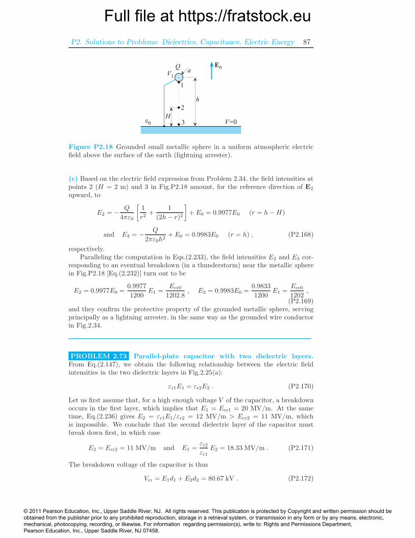
Full file at https://fratstock.euP2. Solutions to Problems: Dielectrics, Capacitance, Electric Energy 87
aE0
V=0e0
V1
Q
1
2
3
h
H
Figure P2.18 Grounded small metallic sphere in a uniform atmospheric electricfield above the surface of the earth (lightning arrester).
(c) Based on the electric field expression from Problem 2.34, the field intensities atpoints 2 (H = 2 m) and 3 in Fig.P2.18 amount, for the reference direction of E2
upward, to
E2 = − Q
4πε0
[1
r2+
1
(2h− r)2]
+ E0 = 0.9977E0 (r = h−H)
and E3 = − Q
2πε0h2+ E0 = 0.9983E0 (r = h) , (P2.168)
respectively.Paralleling the computation in Eqs.(2.233), the field intensities E2 and E3 cor-
responding to an eventual breakdown (in a thunderstorm) near the metallic spherein Fig.P2.18 [Eq.(2.232)] turn out to be
E2 = 0.9977E0 =0.9977
1200E1 =
Ecr0
1202.8, E3 = 0.9983E0 =
0.9833
1200E1 =
Ecr0
1202,
(P2.169)and they confirm the protective property of the grounded metallic sphere, servingprincipally as a lightning arrester, in the same way as the grounded wire conductorin Fig.2.34.
PROBLEM 2.73 Parallel-plate capacitor with two dielectric layers.From Eq.(2.147), we obtain the following relationship between the electric fieldintensities in the two dielectric layers in Fig.2.25(a):
εr1E1 = εr2E2 . (P2.170)
Let us first assume that, for a high enough voltage V of the capacitor, a breakdownoccurs in the first layer, which implies that E1 = Ecr1 = 20 MV/m. At the sametime, Eq.(2.236) gives E2 = εr1E1/εr2 = 12 MV/m > Ecr2 = 11 MV/m, whichis impossible. We conclude that the second dielectric layer of the capacitor mustbreak down first, in which case
E2 = Ecr2 = 11 MV/m and E1 =εr2εr1
E2 = 18.33 MV/m . (P2.171)
The breakdown voltage of the capacitor is thus
Vcr = E1d1 + E2d2 = 80.67 kV . (P2.172)
© 2011 Pearson Education, Inc., Upper Saddle River, NJ. All rights reserved. This publication is protected by Copyright and written permission should be obtained from the publisher prior to any prohibited reproduction, storage in a retrieval system, or transmission in any form or by any means, electronic, mechanical, photocopying, recording, or likewise. For information regarding permission(s), write to: Rights and Permissions Department, Pearson Education, Inc., Upper Saddle River, NJ 07458.
Full file at https://fratstock.eu88 Branislav M. Notaros: Electromagnetics (Pearson Prentice Hall)
PROBLEM 2.74 Parallel-plate capacitor with two dielectric sectors.The electric field intensities in the two dielectric sectors in Fig.2.25(b) are the same,Eq.(2.151), so it is obvious that, after a voltage of critical value is applied acrossthe capacitor plates, a breakdown will occur in the second sector (with a smallerEcr). The corresponding field values are
E2 = Ecr2 = 11 MV/m and E1 = E2 = 11 MV/m < Ecr1 = 20 MV/m ,(P2.173)
and the capacitor breakdown voltage comes out to be
Vcr = E1d = 66 kV . (P2.174)
PROBLEM 2.75 Breakdown in a spherical capacitor with two layers.(a) If the inner dielectric layer of the spherical capacitor in Fig.2.27 is made frommica and the outer layer is oil, Eqs.(2.241) give
Q(1)cr = 4πεr1ε0a
2Ecr1 = 48.07 µC and Q(2)cr = 4πεr2ε0b
2Ecr2 = 24.57 µC .(P2.175)
This means [see Eq.(2.242)] that the breakdown (for sufficiently high applied voltageacross the capacitor) occurs in the outer dielectric layer, and the breakdown valueof the capacitor charge amounts to
Qcr = Q(2)cr = 24.57 µC . (P2.176)
The breakdown voltage is
Vcr =Qcr
Cold= 2.134 MV , (P2.177)
where Cold = 11.52 pF is the capacitance of the capacitor in the first (old) electro-static state (Problem 2.42).
(b) After the oil is drained from the capacitor, so that the outer dielectric layer isnow air, the second charge in Eqs.(P2.175) becomes
Q(2)cr = 4πε0b
2Ecr0 = 2.14 µC (εr2 = 1 , Ecr0 = 3 MV/m) , (P2.178)
indicating that the outer layer breaks down first, again. However, the breakdownvoltage changes, to
Qcr = Q(2)cr = 2.14 µC −→ Vcr =
Qcr
Cnew= 253.7 kV , (P2.179)
with Cnew = 8.44 pF being the capacitance of the capacitor in the new state (Prob-lem 2.42).
© 2011 Pearson Education, Inc., Upper Saddle River, NJ. All rights reserved. This publication is protected by Copyright and written permission should be obtained from the publisher prior to any prohibited reproduction, storage in a retrieval system, or transmission in any form or by any means, electronic, mechanical, photocopying, recording, or likewise. For information regarding permission(s), write to: Rights and Permissions Department, Pearson Education, Inc., Upper Saddle River, NJ 07458.
Full file at https://fratstock.euP2. Solutions to Problems: Dielectrics, Capacitance, Electric Energy 89
PROBLEM 2.76 Breakdown potential of a coated metallic sphere. (a)-(b) For breakdown considerations, the value of the radius c in Fig.2.27 is actually
irrelevant, so it can even be c → ∞; hence, we can reuse the expressions Q(1)cr =
4πεr1ε0a2Ecr1 and Q
(2)cr = 4πε0b
2Ecr0 from the previous problem (for a spherical
capacitor with air as the second dielectric layer), which result in Q(1)cr = 1.33 µC
and Q(2)cr = 0.3 µC. We conclude that the breakdown would occur in air, near the
interface with the dielectric coating of the metallic sphere, and Qcr = Q(2)cr = 0.3 µC
[Eq.(2.242)]. Using the capacitance of the sphere computed in Problem 2.44, C =2.224 pF, the breakdown potential of the sphere and the maximum electric energyof this structure are
Vcr =Qcr
C= 135 kV and We =
Q2cr
2C= 20.2 mJ , (P2.180)
respectively.
PROBLEM 2.77 Breakdown in a coaxial cable with two layers. (a) Letus pursue the first way (based on the direct evaluation of the electric field intensitiesat characteristic locations in the structure) of the breakdown analysis presented fora spherical capacitor with a two-layer dielectric in Example 2.32. For the coaxialcable in Fig.2.50, Eqs.(2.234) and (2.235) take the following form:
E1(r) =Q′
2πεr1ε0r= E1(a
+)a
r(a < r < b) , (P2.181)
E2(r) =Q′
2πεr2ε0r= E2(b
+)b
r(b < r < c) , (P2.182)
and hence the relationship
εr1aE1(a+) = εr2bE2(b
+) . (P2.183)
An assumption that a breakdown occurs in the inner layer leads to
E1(a+) = Ecr1 = 40 MV/m −→ E2(b
+) = Ecr1εr1a
εr2b= 50 MV/m > Ecr2 ,
(P2.184)which is impossible. Hence, an eventual breakdown must be in the outer layer,
E2(b+) = Ecr2 = 20 MV/m −→ E1(a
+) = Ecr2εr2b
εr1a= 16 MV/m < Ecr1 .
(P2.185)Similarly to Eq.(2.240), the breakdown voltage of the cable is computed, using
the field-intensity values in Eqs.(P2.185), as
Vcr = E1(a+) a
∫ b
a
dr
r+E2(b
+) b
∫ c
b
dr
r= εr2bEcr2
(1
εr1lnb
a+
1
εr2lnc
b
)
= 38.8 kV .
(P2.186)
(b) The maximum energy that the cable can store per unit of its length amounts to
W ′e =
1
2C′V 2
cr = 86.4 mJ/m , (P2.187)
© 2011 Pearson Education, Inc., Upper Saddle River, NJ. All rights reserved. This publication is protected by Copyright and written permission should be obtained from the publisher prior to any prohibited reproduction, storage in a retrieval system, or transmission in any form or by any means, electronic, mechanical, photocopying, recording, or likewise. For information regarding permission(s), write to: Rights and Permissions Department, Pearson Education, Inc., Upper Saddle River, NJ 07458.
Full file at https://fratstock.eu90 Branislav M. Notaros: Electromagnetics (Pearson Prentice Hall)
where C′ = 114.7 pF/m is the capacitance p.u.l. of the cable, found in Problem2.48.
PROBLEM 2.78 Simultaneous breakdown in two spherical layers. Fora sufficiently large applied voltage, dielectric breakdown will occur in both dielec-tric layers in the capacitor in Fig.2.27 simultaneously if the two values of charges
Q(1)cr and Q
(2)cr in Eqs.(2.241) are the same, which condition results in the following
relationship between the parameters of the capacitor:
Q(1)cr = Q(2)
cr −→ εr1a2Ecr1 = εr2b
2Ecr2 . (P2.188)
PROBLEM 2.79 Simultaneous breakdown in two coaxial layers. Let usconsider the critical value, for breakdown, of the charge Q′ per unit length of thecoaxial cable in Fig.2.50, and denote by Q′
cr1 and Q′cr2 the charge Q′ in the case
of an eventual breakdown in the inner and outer dielectric layers, respectively, ofthe cable. Based on the breakdown analysis in Problem 2.77, we then obtain thefollowing expressions for these charges, analogous to those in Eqs.(2.241) for thecorresponding spherical capacitor:
Q′cr1 = 2πεr1ε0aEcr1 and Q′
cr2 = 2πεr2ε0bEcr2 . (P2.189)
Hence, we conclude that the breakdown will occur in both dielectric layers inFig.2.50 simultaneously if
Q′cr1 = Q′
cr2 −→ εr1aEcr1 = εr2bEcr2 . (P2.190)
PROBLEM 2.80 Metallic sphere half immersed in a liquid dielectric.Denoting by Vcr the maximum potential of the metallic sphere in Fig.2.49 such thatdielectric breakdown will not occur after it is removed from the liquid and raisedin air high above the interface, the corresponding critical value of the charge of thesphere, using the expression for its capacitance from Problem 2.47, turns out to be
Qcr = CVcr = 2π(εr + 1)ε0aVcr . (P2.191)
This charge remains the same upon the elevation of the sphere above the liquid.
In the new electrostatic state, assuming that the sphere is isolated in air (as itis high above the interface), the condition for a breakdown near the sphere surface,expressed as in Problem 2.69, actually determines the value of Qcr, as follows:
Qcr = 4πε0a2Ecr0 (Ecr0 = 3 MV/m) . (P2.192)
Substituted back in Eq.(P2.191), for the first electrostatic state, it leads to
Vcr =2aEcr0
εr + 1= 30 kV . (P2.193)
© 2011 Pearson Education, Inc., Upper Saddle River, NJ. All rights reserved. This publication is protected by Copyright and written permission should be obtained from the publisher prior to any prohibited reproduction, storage in a retrieval system, or transmission in any form or by any means, electronic, mechanical, photocopying, recording, or likewise. For information regarding permission(s), write to: Rights and Permissions Department, Pearson Education, Inc., Upper Saddle River, NJ 07458.
Full file at https://fratstock.euP2. Solutions to Problems: Dielectrics, Capacitance, Electric Energy 91
Finally, we need yet to check whether the system in Fig.2.49 is safe from break-down in the first state. The electric field intensity near the sphere surface in boththe liquid and air is, from Eqs.(2.175) and (P2.192),
E(a+) =Qcr
2π(εr + 1)ε0a2=
2Ecr0
εr + 1=Ecr0
2= 1.5 MV/m . (P2.194)
Since E(a+) < Ecr0 (for air) and E(a+) < Ecr = 20 MV/m (for the liquid dielec-tric), we conclude that setting the sphere to the potential Vcr or charging it with Qcr
while half in the liquid (in the first state) will not cause breakdown of the system,which will occur only after the sphere is raised in air.
PROBLEM 2.81 Breakdown in a coaxial cable with a dielectric spacer.(a) The electric field intensity near the inner conductor of the cable in Fig.2.33 isgiven by the expression in Eq.(2.218). This, for r = a+, is the largest electric fieldintensity in the cable. Since it is the same in both the dielectric spacer and theair-filled part of the cable interior, an eventual dielectric breakdown will occur inair (Ecr0 < Ecr), if
E(a+) =Vcr
a ln(b/a)= Ecr0 = 3 MV/m , (P2.195)
and hence the breakdown voltage of the cable
Vcr = Ecr0 a lnb
a= 6.59 kV . (P2.196)
(b) Having in mind Eqs.(2.178), as well as the capacitance found in Problem 2.50,the capacitance per unit length of the cable (Fig.2.33) is
C′ =εrε0α+ ε0(2π − α)
ln(b/a)=
(εrπ/3 + 5π/3) ε0ln(b/a)
= 84.4 pF/m , (P2.197)
so that the electric energy per unit length of the cable at breakdown amounts to
W ′e =
1
2C′V 2
cr = 1.83 mJ/m . (P2.198)
© 2011 Pearson Education, Inc., Upper Saddle River, NJ. All rights reserved. This publication is protected by Copyright and written permission should be obtained from the publisher prior to any prohibited reproduction, storage in a retrieval system, or transmission in any form or by any means, electronic, mechanical, photocopying, recording, or likewise. For information regarding permission(s), write to: Rights and Permissions Department, Pearson Education, Inc., Upper Saddle River, NJ 07458.