Printed from file Rouen-2010/Quantum/finite-elements.tex on November 11, 2010

From Wave Mechanics to Matrix Mechanics:

The Finite Element Method

Robert Gilmore

1 The Origin of Wave Mechanics

Schrodinger originally formulated Wave Mechanics as a variational problem:

δ

∫ (

~2

2m(∇ψ)∗(∇ψ) + ψ∗V (x)ψ − ψ∗Eψ

)

d3x = 0 (1)

There are only a few analytic solutions available for this partial differential equation. Schrodingerfound all of the most useful ones in his first paper on Quantum Mechanics: the Coulomb potentialand the harmonic oscillator potential. He published the solution to the nonrelativistic Coulombproblem in his first Wave Mechanics paper but solved the relativistic problem six months earlier.He also solved the harmonic oscillator problem in his first paper and introduced what are now calledcoherent states in another paper six months afterward.

With the advent of powerful computers and even more powerful linear algebra algorithms, partialdifferential equations are usually solved by first transforming them into matrix equations and thensolving the matrix equations. Solutions almost always involve either matrix inversion or matrixdiagonalization.

The Schrodinger equation is usually not given in the original variational form. It is usuallyexpressed as a second order partial differential equation. The relation between the two is obtainedas follows. The kinetic energy term is integrated by parts:

∫ ∇ψ∗ · ∇ψ2m(x)

dV =

∫

∇·(

ψ∗∇ψ2m(x)

)

dV −∫

ψ∗∇·( ∇ψ

2m(x)

)

dV =

∫

∂V

(

ψ∗∇ψ2m(x)

)

·dS−∫

ψ∗∇·( ∇ψ

2m(x)

)

dV

(2)When the surface integral vanishes, the kinetic energy term in the variational expression can bereplaced by the negative of the Laplacian. The variational expression is now

δ

∫

ψ∗(x)

(

−~2∇·

(∇ψ(x)

2m(x)

)

+ V (x)ψ − Eψ

)

d3x = 0 (3)

The functions ψ(x) and ψ∗(x) can be varied independently. Varying ψ∗(x) leads to “the” Schrodingerequation:

−~2∇·

(∇ψ(x)

2m(x)

)

+ V (x)ψ − Eψ = 0 (4)

When m(x) is a constant this equation assumes its universally recognized form. In many cases theeffective mass m(x) is not constant: for example, in solids where the effective mass is a surrogate for

1

−1−0.5

00.5

1

−0.5

0

0.50

0.1

0.2

0.3

0.4

0.5

0.6

0.7

Color: u Height: u

0.1

0.2

0.3

0.4

0.5

0.6

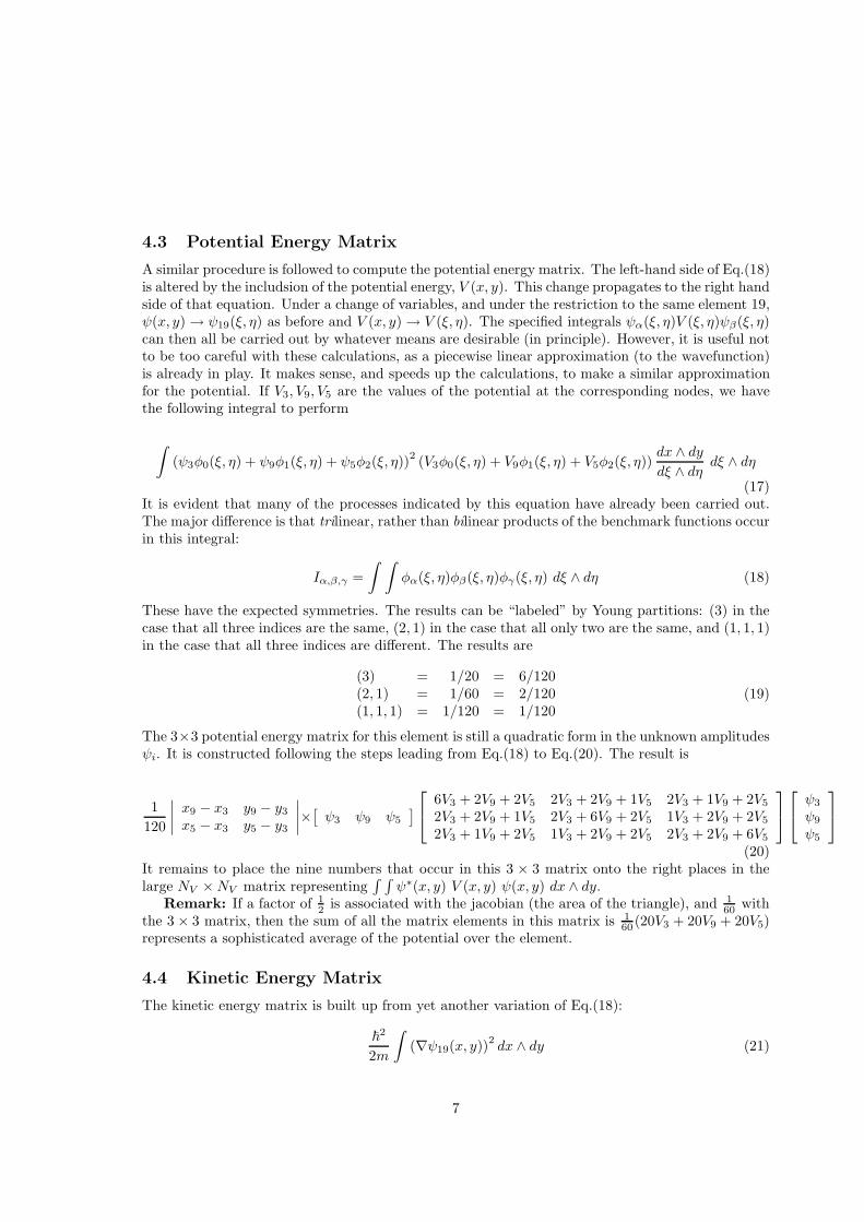
Figure 1: The ground state wavefunction for a particle trapped in an infinitely deep two-dimensionalpotential well has been evaluated at a small number of points and a 3D plot constructed from thetriples of values (xi, yi, ψi). The wavefunction is linearly interpolated between triples of nearbypoints. This faceted representation provides an “accurate” understanding of the wavefunction.

many electron effects. In such cases it is important to recognize that continuity conditions acrossboundaries should be imposed on the wavefunction ψ(x) and on the velocity ∇ψ(x)/m(x), not onthe momentum ∇ψ(x).

Today, if we wanted to visualize a wavefunction, we would try to display it on a computerscreen. To do this, we would have to determine its value at a discrete set of points (x, y)i in theplane and then construct a “3D” plot (xi, yi, ψi), where ψi = ψ(xi, yi). Many plotting routinesroutinely interpolate values the the function being plotted between the points at which the functionis evaluated. Such a visualization is shown in Fig. 1.

The purpose of Fig. 1 is to emphasize that the eigenfunction is well-represented if its value isknown at a lot of nearby points.

The idea underlying the finite element method (in 2D) is to replace the problem of determiningthe wavefunction ψ(x, y) at all (x, y) (basically by solving a PDE) by the problem of determiningonly a sample of values ψi at a discrete set of points (x, y)i (basically by solving a matrix eigenvalueequation).

2 Tesselation

The first step in applying the finite element method is to determine the points at which the wave-function is to be evaluated. To this end the region of space (1D, 2D, 3D, ...) of interest is determined.A boundary is placed on or around this region. Then a set of points is distributed throughout thisbounded region, including on the boundary itself. There is a Goldilocks problem here. If too fewpoints are used we will construct a poor representation of the wavefunction. If too many points

2

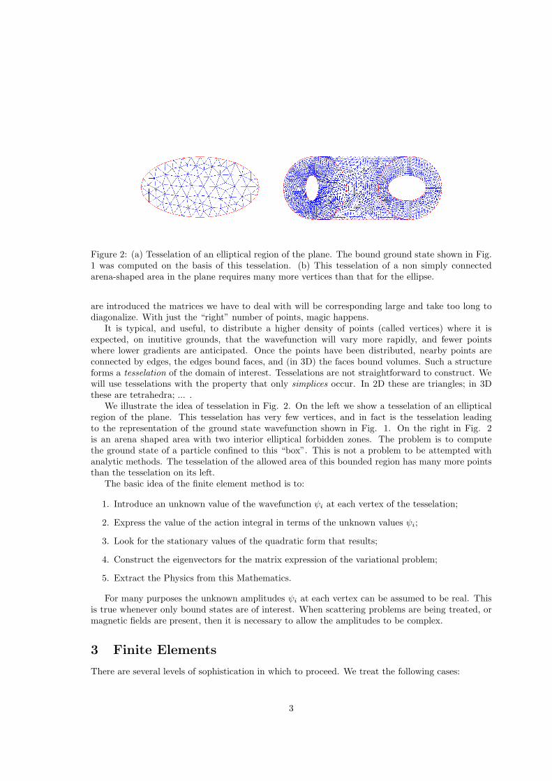
Figure 2: (a) Tesselation of an elliptical region of the plane. The bound ground state shown in Fig.1 was computed on the basis of this tesselation. (b) This tesselation of a non simply connectedarena-shaped area in the plane requires many more vertices than that for the ellipse.

are introduced the matrices we have to deal with will be corresponding large and take too long todiagonalize. With just the “right” number of points, magic happens.

It is typical, and useful, to distribute a higher density of points (called vertices) where it isexpected, on inutitive grounds, that the wavefunction will vary more rapidly, and fewer pointswhere lower gradients are anticipated. Once the points have been distributed, nearby points areconnected by edges, the edges bound faces, and (in 3D) the faces bound volumes. Such a structureforms a tesselation of the domain of interest. Tesselations are not straightforward to construct. Wewill use tesselations with the property that only simplices occur. In 2D these are triangles; in 3Dthese are tetrahedra; ... .

We illustrate the idea of tesselation in Fig. 2. On the left we show a tesselation of an ellipticalregion of the plane. This tesselation has very few vertices, and in fact is the tesselation leadingto the representation of the ground state wavefunction shown in Fig. 1. On the right in Fig. 2is an arena shaped area with two interior elliptical forbidden zones. The problem is to computethe ground state of a particle confined to this “box”. This is not a problem to be attempted withanalytic methods. The tesselation of the allowed area of this bounded region has many more pointsthan the tesselation on its left.

The basic idea of the finite element method is to:

1. Introduce an unknown value of the wavefunction ψi at each vertex of the tesselation;

2. Express the value of the action integral in terms of the unknown values ψi;

3. Look for the stationary values of the quadratic form that results;

4. Construct the eigenvectors for the matrix expression of the variational problem;

5. Extract the Physics from this Mathematics.

For many purposes the unknown amplitudes ψi at each vertex can be assumed to be real. Thisis true whenever only bound states are of interest. When scattering problems are being treated, ormagnetic fields are present, then it is necessary to allow the amplitudes to be complex.

3 Finite Elements

There are several levels of sophistication in which to proceed. We treat the following cases:

3

Section 3: 2 dimensions, linear basis functions.

Section 4: 3 dimensions, linear basis functions.

Section 5: 2 dimensions, cubic basis functions.

Section 6: 3 dimensions, cubic basis functions.

We first describe a simple case. A potential acts on a particle of mass m in a localized region in 2D. A region in two dimensions containing the potential is tesselated by choosing a sufficient numberof vertices. The vertices are uniquely identified — usually through an integer i that ranges from1 to NV . The region is divided into adjacent areas; each area is called an element. The elementsare also uniquely identified — usually through an integer α that ranges from 1 to NE . The three(or more) vertices that define the edges of each element are associated with that element througha list. Another list contains information about the coordinates of each vertex. The behavior ofa wavefunction in each element is represented by a linear combination of basis functions that arenonzero only in that element.

If the ultimate objective is to determine the wavefunction, and it is required to have the wave-function be continuous but there is no concern about having the derivatives across elements becontinuous, we are in one domain of simplicity. We describe what happens in this domain and letthe complications pile on later.

Within an element with 3 vertices we choose 3 basis functions. Each has value +1 at one ofthe three vertices and vanishes at the other two. These three functions are defined only within thatsingle element. To put it another way, they are defined to be zero outside that specific element.

It is useful in principle to take the three basis functions to be linear combinations of the constant1 and the coordinates x and y (that is not what we do). If we do this the wave function can bewritten

ψ(x) =

NE∑

α=1

ψα(x) (5)

Here ψα(x) is zero outside the element α and nonzero only inside this element. In fact, it linearlyinterpolates between the (unknown) values of the wavefunction at the three coordinates.

The terms in the variational expression Eq.(1) simplify. For example

∫

ψ∗(x)Eψ(x)dx =

∫

(

NE∑

α=1

ψα(x)

)

E

NE∑

β=1

ψβ(x)

dx = E

NE∑

α=1

∫

ψ∗α(x)ψα(x) dx (6)

The collapse of the double sum to a single sum in the last equation comes about because ψα(x) iszero where ψβ(x) is nonzero, unless α = β. This is true also for derivatives of either or both of thesefunctions.

The wave function ψα(x) will be “cooked up” to interpolate linearly between the values that ψ(x)assumes at the three vertices that define the element α. As a result, ψα(x) will depend linearly onthese three values, and the expectation value in Eq.(10) will be a quadratic form in these unknowns.

The potential energy term is treated similarly:

∫

ψ∗(x)V (x)ψ(x)dx =

∫

(

NE∑

α=1

ψα(x)

)

V (x)

NE∑

β=1

ψβ(x)

dx =

NE∑

α=1

∫

ψ∗α(x)V (x)ψα(x) dx (7)

4

The same goes for the kinetic energy term:

~2

2m

∫

∇ψ∗(x)∇ψ(x)dx =~

2

2m

∫

(

NE∑

α=1

∇ψα(x)

)∗

NE∑

β=1

∇ψβ(x)

dx =~

2

2m

NE∑

α=1

∫

∇ψ∗α(x)∇ψα(x) dx

(8)All three expressions, Eqs. (10 - 12), are quadratic forms in the unknown values of the wavefunctionat the vertices defining the element α.

This is the general outline. The devil is in the details. So we now illustrate the workings of thismethod by outlining an example.

4 2D: Linear Functions

The equations above show that there are a lot of integrals to do. Ultimately, each integral will beexpressed as a quadratic form in the values of ψ at the vertices, multiplied by some function of thecoordinates of the vertices. These fucntions are closely related to each other. to simplify life, weproceed as follows. First we define a benchmark simplex. This will be a right triangle in the ξ − ηplane. The coordinates of the vertices of this right triangle are (0, 0), (1, 0), and (0, 1) (see Fig. 3).We take as three basis functions in this benchmark triangle

φ0 = 1 − ξ − ηφ1 = ξφ2 = η

(9)

These three functions have the desired properties

Value at (0, 0) Value at (1, 0) Value at (0, 1)φ0(ξ, η) 1 0 0φ1(ξ, η) 0 1 0φ2(ξ, η) 0 0 1

(10)

The integrals in Eqs. (10 - 12) are most simply done by using the chain rule to change variables.The change of variables is a simple linear transformation, so the integrals can be transformed fromthe “real” (x, y) space to the “benchmark” (ξ, η) space, where they need be worked out only once.Since the transformation is linear, the jacobian of the transformation is a constant that can beremoved from all integrals.

4.1 Structure of Approximation

Here goes. Set up 3 matrices. Each is NV ×NV in size, with rows and columns labeled by the index(i) used to identify the different vertices.

Choose an element, say α = 19. From the list of elements and their vertices, determine the 3vertices associated with element 19. Let’s say they are 3, 5, and 9. Change variables from (x, y) to(ξ, η) as follows:

(x, y)3 → (0, 0)(x, y)9 → (1, 0)(x, y)5 → (0, 1)

ξ =

∣

∣

∣

∣

x− x3 y − y3x5 − x3 y5 − y3

∣

∣

∣

∣

∣

∣

∣

∣

x9 − x3 y9 − y3x5 − x3 y5 − y3

∣

∣

∣

∣

η =

∣

∣

∣

∣

x9 − x3 y9 − y3x− x3 y − y3

∣

∣

∣

∣

∣

∣

∣

∣

x9 − x3 y9 − y3x5 − x3 y5 − y3

∣

∣

∣

∣

(11)

5

At this point it is very useful to express the linear transformation between coordinates (x, y) inthe physical space and the coordinates (ξ, η) in the benchmark space in terms of the 2 × 2 matrix[J ] whose determinant appears in the denominators above:

(

x− x3 y − y3)

=(

ξ η)

[

x9 − x3 y9 − y3x5 − x3 y5 − y3

]

↔[

∂/∂ξ∂/∂η

]

=

[

x9 − x3 y9 − y3x5 − x3 y5 − y3

] [

∂/∂x∂/∂y

]

(12)The dual relation that exists between transformations of coordinates and derivatives with respectto these coordinates is a consequence of co- and contra-variance.

Next, we approximate ψ(x, y) within element 19 by a linear combination of the benchmarkfunctions within the benchmark triangle:

ψ19(x, y) → ψ3φ0(ξ, η) + ψ9φ1(ξ, η) + ψ5φ2(ξ, η) (13)

The three coefficients(ψ3, ψ9, ψ5) are at present unknown, as are all the other values ψi of ψ(x, y) atthe vertices.

4.2 Matrix of Overlap Integrals

Now we compute∫

|ψ19(x, y)|2dx∧dy over the element 19 by exploiting the linear change of variables:

∫

ψ19(x, y)2dx ∧ dy =

∫

(ψ3φ0(ξ, η) + ψ9φ1(ξ, η) + ψ5φ2(ξ, η))2 dx ∧ dydξ ∧ dη dξ ∧ dη (14)

Since ξ and η are linear in x and y the jacobian dx∧dydξ∧dη = |J | is constant. This is the ratio of

the physical triangle with vertices 3, 9, 5 to the benchmark right triangle with vertices 0, 1, 2. Theabsolute value of this constant may be taken out of the integral. Remaining inside the integral arebilinear products of the three functions φk(ξ, η) and bilinear products of the three unknowns ψi andtheir complex conjugates. The functions of (ξ, η) can be integrated once and for all. The matrix ofinner products is

∫ ∫

φi(ξ, η)φj(ξ, η) dξ ∧ dη =

1

12

1

24

1

241

24

1

12

1

241

24

1

24

1

12

(15)

Putting all these results together, the contribution to the overlap matrix from vertices (3, 9, 5) ofelement 19 is:

1

24

∣

∣

∣

∣

x9 − x3 y9 − y3x5 − x3 y5 − y3

∣

∣

∣

∣

×[

ψ3 ψ9 ψ5

]∗

2 1 11 2 11 1 2

ψ3

ψ9

ψ5

(16)

It remains to place the nine numbers that occur in this 3 × 3 matrix onto the right places in thelarge NV ×NV matrix representing

∫ ∫

ψ∗(x, y) E ψ(x, y) dx ∧ dy.Remark: For bound states the wave functions can be taken real, so the bilinear form in the

amplitudes ψ∗i , ψj can be taken as a quadratic form in the real amplitudes ψj . This is true for bound

states. For scattering states, and when magnetic fields are present, the amplitudes ψi are in generalcomplex and cannot be made real.

6

4.3 Potential Energy Matrix

A similar procedure is followed to compute the potential energy matrix. The left-hand side of Eq.(18)is altered by the includsion of the potential energy, V (x, y). This change propagates to the right handside of that equation. Under a change of variables, and under the restriction to the same element 19,ψ(x, y) → ψ19(ξ, η) as before and V (x, y) → V (ξ, η). The specified integrals ψα(ξ, η)V (ξ, η)ψβ(ξ, η)can then all be carried out by whatever means are desirable (in principle). However, it is useful notto be too careful with these calculations, as a piecewise linear approximation (to the wavefunction)is already in play. It makes sense, and speeds up the calculations, to make a similar approximationfor the potential. If V3, V9, V5 are the values of the potential at the corresponding nodes, we havethe following integral to perform

∫

(ψ3φ0(ξ, η) + ψ9φ1(ξ, η) + ψ5φ2(ξ, η))2(V3φ0(ξ, η) + V9φ1(ξ, η) + V5φ2(ξ, η))

dx ∧ dydξ ∧ dη dξ ∧ dη

(17)It is evident that many of the processes indicated by this equation have already been carried out.The major difference is that trilinear, rather than bilinear products of the benchmark functions occurin this integral:

Iα,β,γ =

∫ ∫

φα(ξ, η)φβ(ξ, η)φγ(ξ, η) dξ ∧ dη (18)

These have the expected symmetries. The results can be “labeled” by Young partitions: (3) in thecase that all three indices are the same, (2, 1) in the case that all only two are the same, and (1, 1, 1)in the case that all three indices are different. The results are

(3) = 1/20 = 6/120(2, 1) = 1/60 = 2/120(1, 1, 1) = 1/120 = 1/120

(19)

The 3×3 potential energy matrix for this element is still a quadratic form in the unknown amplitudesψi. It is constructed following the steps leading from Eq.(18) to Eq.(20). The result is

1

120

∣

∣

∣

∣

x9 − x3 y9 − y3x5 − x3 y5 − y3

∣

∣

∣

∣

×[

ψ3 ψ9 ψ5

]

6V3 + 2V9 + 2V5 2V3 + 2V9 + 1V5 2V3 + 1V9 + 2V5

2V3 + 2V9 + 1V5 2V3 + 6V9 + 2V5 1V3 + 2V9 + 2V5

2V3 + 1V9 + 2V5 1V3 + 2V9 + 2V5 2V3 + 2V9 + 6V5

ψ3

ψ9

ψ5

(20)It remains to place the nine numbers that occur in this 3 × 3 matrix onto the right places in thelarge NV ×NV matrix representing

∫ ∫

ψ∗(x, y) V (x, y) ψ(x, y) dx ∧ dy.Remark: If a factor of 1

2is associated with the jacobian (the area of the triangle), and 1

60with

the 3 × 3 matrix, then the sum of all the matrix elements in this matrix is 1

60(20V3 + 20V9 + 20V5)

represents a sophisticated average of the potential over the element.

4.4 Kinetic Energy Matrix

The kinetic energy matrix is built up from yet another variation of Eq.(18):

~2

2m

∫

(∇ψ19(x, y))2dx ∧ dy (21)

7

The components of the gradient are computed using the chain rule: that is, the linear relationamong partial derivatives given is Eq.(16). We apply the column vector of physical derivatives to thefunction ψ(x, y) and the column vector of benchmark derivatives ∂/∂ξ, ∂/∂η to the representationψ3φ0(ξ, η) + ψ9φ1(ξ, η) + ψ5φ2(ξ, η), obtaining

[

∂ψ/∂x∂ψ/∂y

]

= J−1

[

ψ9 − ψ3

ψ5 − ψ3

]

(22)

The inner product of the gradient of the wavefunction with itself is

(∇ψ)·(∇ψ) =[

∂ψ/∂x ∂ψ/∂y]

[

∂ψ/∂x∂ψ/∂y

]

=[

ψ9 − ψ3 ψ5 − ψ3

]

(J−1)tJ−1

[

ψ9 − ψ3

ψ5 − ψ3

]

(23)If we define matrix elements A,B,C of the real symmetric matrix (J−1)tJ−1 = (JJ t)−1 as describedbelow, the conversion to a 3 × 3 matrix of the quadratic form for the three coefficients ψ3, ψ9, ψ5 isquickly determined:

[

ψ9 − ψ3 ψ5 − ψ3

]

[

A BB C

] [

ψ9 − ψ3

ψ5 − ψ3

]

=[

ψ3 ψ9 ψ5

]

A+ 2B + C −A−B −B − C−A−B A B−B − C B C

ψ3

ψ9

ψ5

(24)This constant must be integrated over the area of simplex 19 with vertices 3, 9, 5. The volume is

1

2!|J |. The 9 elements in this 3× 3 matrix are constructed by computing the matrix J , inverting the

matrix JJ t, and spreading out the 4 = 22 elements of this symmetric matrix in the proper way toconstruct the 9 = 32 matrix elements for the kinetic energy contribution on element 19. All matrixelements must be multiplied by the positive area factor 1

2!|J |.

It remains to place the nine numbers that occur in this 3 × 3 matrix in Eq.(28) onto the right

places in the large NV ×NV matrix representing ~2

2m

∫ ∫

(∇ψ(x, y))∗(∇ψ(x, y)) dx ∧ dy.Remark 1: The procedure for constructing the matrix in Eq.(28) is algorithmic in five simple

steps.1. Construct a jacobian matrix as the difference in the x and y coordinates of the triple of

vertices defining a triangular element, as shown in Eq.(16).2. Construct the transpose of this matrix.3. Compute the product (JJ t).4. Compute the inverse of this 2 × 2 matrix.5. Spread the 4 matrix elements of this inverse out into 9 matrix elements, as shown in Eq.(28).This is a very fast and efficient algorithm.Remark 2: This result is aesthetically unsatisfying in that it appears to treat the three vertices

asymmetrically. The result is symmetric in the coordinates, despite the appearance of Eq.(28). Toshow this it is useful to write down the explicit form the the three independent matrix elementsA,B,C in terms of the 2 coordinates of each of the 3 vertices: A = ∆x20·∆x20, C = ∆x01·∆x01,B = −∆x10·∆x20. Here, to reduce complexity of notation, the three vertices are labeled 1, 2, 3 and∆x21·∆x31 = (x2 − x1)(x3 − x1) + (y2 − y1)(y3 − y1), etc. When these expressions are placed intothe 3 × 3 matrix in Eq.(28), the form for the 11, 1i, and i1 matrixd elements immediately suggestsitself:

+∆x23·∆x23 −∆x13·∆x23 −∆x12·∆x32

−∆x23·∆x13 +∆x31·∆x31 −∆x21·∆x31

−∆x32·∆x12 −∆x31·∆x21 +∆x12·∆x12

(25)

8

This matrix is symmetric in the coordinates of the vertex triple!Remark 3: The local 3 × 3 kinetic energy matrix should be multiplied by a constant (~2/2m)

before it is placed in the NV ×NV kinetic energy matrix. If the mass m is the same in all elements,this multiplication can be postponed until the entire NV ×NV kinetic energy matrix is constructed,and then this multiplication can be carried out. On the other hand, if m = m(x) is not the samethroughout the region of interest, then multiplication by ~

2/2melement must be carried out on anelement by element basis.

4.5 Magnetic Matrix

An additional contribution is necessary when magnetic fields are present. If spin is not explicitlytaken into account, all magnetic interactions are accounted for by the Principle of Minimal Electro-magnetic Coupling. This is to replace p by p− q

cA in the Hamiltonian. Opening up (p− qcA)2 leads

to four terms. Two of them, p · p and A · A, are handled as described above in Eqs. (20) and (24).The remaining two terms are cross terms of the form p ·A and A · p. We will derive an expressionfor ∇ ·A. The expression for A · ∇ will be its transpose. These expressions must be multiplied by(

1

2m × ~

i × −qc

)∗and

(

1

2m × ~

i × −qc

)

before being placed into the appropriate matrix elements ofthe magnetic matrix.

The expression that must be computed is

∫

(∇ψ19)∗·(Aψ19) dx ∧ dy (26)

In order to evaluate the first term on the left we use the results in Eq. (22):

(∇ψ19)∗ =

[

∂ψ/∂x ∂ψ/∂y]∗

=[

ψ9 − ψ3 ψ5 − ψ3

]∗(J−1)t (27)

If we write (J−1)t =

[

A BC D

]

then the expression on the right of this equation can be expressed

as

[

ψ3 ψ9 ψ5

]∗

−A− C −B −DA BC D

=[

ψ3 ψ9 ψ5

]∗

∗ ∗

(J−1)t

(28)

In this expression the entries * indicate that the choice of this matrix element is such that eachcolumn sum is zero. These terms are independent of the coordinate, so may be taken out of theintegral.

The right hand side of the integral in Eq. (26) is now

dx ∧ dydξ ∧ dη

[

Ax3φ0 +Ax9φ1 +Ax5φ2

Ay3φ0 +Ay9φ1 +Ay5φ2

]

× (ψ3φ0 + ψ9φ1 + ψ5φ2) dξ ∧ dη (29)

The integrals involve only pairwise products of the basis functions φi, so all are represented by thematrix Mij in Eq.(15). When these results are collected we find the following bilinear expression inthe amplitudes ψ∗ and ψ:

[

ψ3 ψ9 ψ5

]∗ |J |

∗ ∗

(J−1)t

[

Ax3 Ax9 Ax5

Ay3 Ay9 Ay5

]

1

24

2 1 11 2 11 1 2

ψ3

ψ9

ψ5

(30)

9

The matrix elements of the 3 × 3 matrix must be multiplied by −(~/i)∗(q/2mc) and then placedinto the appropriate spots of the NV ×NV magnetic matrix.

The matrix elements of A · ∇ are obtained from the transpose of the 3 × 3 matrix in Eq. (30):

[

ψ3 ψ9 ψ5

]∗ |J | 1

24

2 1 11 2 11 1 2

Ax3 Ay3

Ax9 Ay9

Ax5 Ay5

∗(J−1)

∗

ψ3

ψ9

ψ5

(31)

This must be multiplied by −(~/i)(q/2mc) and then placed into the appropriate spots of theNV ×NV

magnetic matrix. The resulting magnetic matrix is hermitian: it is an imaginary antisymmetricmatrix.

4.6 Implementing the Details

Introduce the potential V (x, y) and decide on the region of the plane which is of interest. Tesselatethis region with vertices and number the vertices from 1 to NV . Store information about the x andy coordinates of each vertex. Evaluate and store the value of the potential at each vertex. Numberthe 2-dimensional elements (simplices, or triangles) from 1 to NE. For each element, identify thethree vertices at the “corners”.

Create three NV × NV matrices: an overlap matrix, a potential energy matrix, and a kineticenergy matrix. Zero out each.

Scan through the elements from the first α = 1 to the last α = NE. For each element (e.g.,α = 19) determine its three vertices (e.g., i = 3, 9, 5). For these three vertices compute 3 × 3matrices

Overlap Integral: Eq.(20).

Potential Energy: Eq.(24).

Kinetic Energy: Eq.(28).

Magnetic Energy: Eq.(30).

Add the 9 matrix elements from Eq.(20) into the appropriate places of the NV ×NV overlap matrix.Do the same for the other three matrices from Eq.(24) and Eq.(28). The resulting quadratic formin the unknown amplitudes must be stationary to satisfy the variational principle. This means thatthe generalized eigenvalue equation

〈i|(KE + PE +ME − E)|j〉〈j|ψ〉 = (H−E)ijψj = 0 (32)

must be solved. Here 〈i|∗|j〉 are the matrix elements of the kinetic energy, potential energy, magneticenergy and overlap matrices, respectively, and the row and column indices identify nodes.

As usual, the results should be sorted by energy, tested for convergence, and then plotted.Remark: We should open the possibility of computing matrices for terms of the form p ·A + A · p

because it is likely to be impossible to coax Matlab to do such calculations for us. These are theinteresting type that involve magnetic fields.

10

5 Matrix Variational Problem

The variational problem of Eq.(1) has now been expressed in matrix form as follows:

δ (ψi(H−E)ijψj) = 0 ⇒ (H−E)ijψj = 0 (33)

The variational equation leads directly and immediately to a matrix eigenvalue equation. Since the“diagonal matrix” 〈i|E|j〉 is not diagonal, this is a “generalized eigenvalue problem.”

5.1 Boundary Conditions

The general boundary condition for bound states is that the wavefunction must be square integrable.This means that the square of the wavefunction must go zero more quickly than 1/rD−1, where Dis the dimension of the problem.

5.1.1 Unbounded Domain

To check whether any of the solutions might be considered of any value, it is useful to make thefollowing test. Divide the vertices up into two subsets: the internal vertices, labeled with indicesr, s, .. and the vertices on the boundary, labeled with indices β, κ, ... Check the ratio

∑

β

|ψβ |2/∑

r

|ψr|2 (34)

If this ratio is not small the wavefunction is meaningless. If the ratio is very small the wavefunctionmight carry physical meaning.

5.1.2 Bounded Domain

In this case the variational problme takes the form

δ (ψr(H−E)rsψs + ψr(H−E)rκψκ + ψβ(H−E)βsψs + ψβ(H−E)βκψκ) = 0 (35)

If the potential is infinite outside the domain of interest, the wavefunction vanishes on the boundary.It is necessary to set all components ψβ , ψκ = 0. As a result the last three terms in the expressionabove vanish, and the variation must be done only over the values of the wavefucntion at the interiornodes.

5.1.3 Poisson’s Equation

In some cases it is necessary to solve Poisson’s Equation

∇2Φ = −4πρ (36)

where Φ is an unknown electrostatic potential and ρ is a known charge distribution. The finiteelement is easily modified to treat this problem. The “kinetic energy” matrix for Φ is evaluated asdescribed above. The “diagonal” matrix for ρ is also evaluated (it is the overlap matrix). This leadsto the algebraic equation

(

∇2)

ijΦj = −4πρi (37)

Now a matrix inversion is called for, rather than a matrix diagonalization.

11

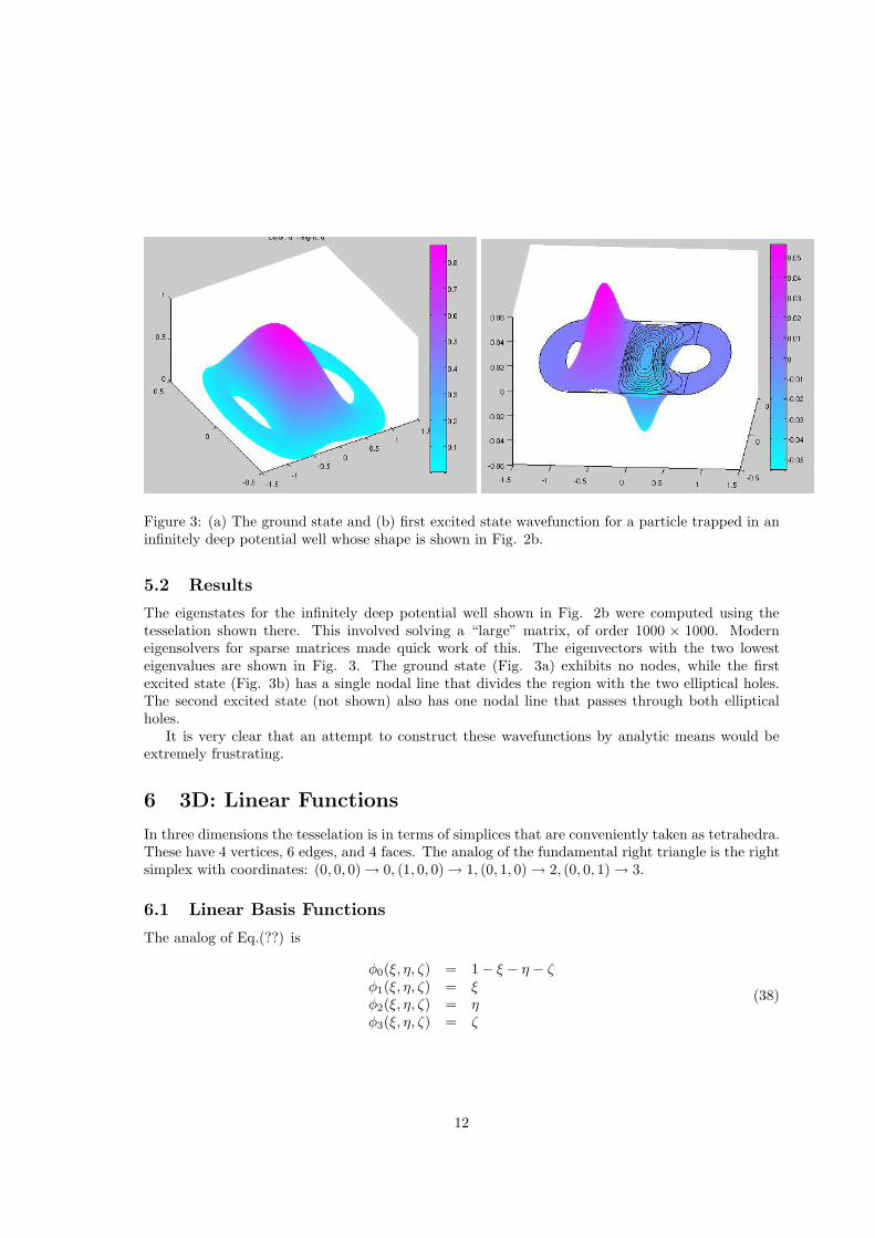
Figure 3: (a) The ground state and (b) first excited state wavefunction for a particle trapped in aninfinitely deep potential well whose shape is shown in Fig. 2b.

5.2 Results

The eigenstates for the infinitely deep potential well shown in Fig. 2b were computed using thetesselation shown there. This involved solving a “large” matrix, of order 1000 × 1000. Moderneigensolvers for sparse matrices made quick work of this. The eigenvectors with the two lowesteigenvalues are shown in Fig. 3. The ground state (Fig. 3a) exhibits no nodes, while the firstexcited state (Fig. 3b) has a single nodal line that divides the region with the two elliptical holes.The second excited state (not shown) also has one nodal line that passes through both ellipticalholes.

It is very clear that an attempt to construct these wavefunctions by analytic means would beextremely frustrating.

6 3D: Linear Functions

In three dimensions the tesselation is in terms of simplices that are conveniently taken as tetrahedra.These have 4 vertices, 6 edges, and 4 faces. The analog of the fundamental right triangle is the rightsimplex with coordinates: (0, 0, 0) → 0, (1, 0, 0) → 1, (0, 1, 0) → 2, (0, 0, 1) → 3.

6.1 Linear Basis Functions

The analog of Eq.(??) is

φ0(ξ, η, ζ) = 1 − ξ − η − ζφ1(ξ, η, ζ) = ξφ2(ξ, η, ζ) = ηφ3(ξ, η, ζ) = ζ

(38)

12

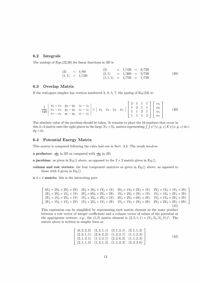
6.2 Integrals

The analogs of Eqs.(22,26) for linear functions in 3D is

(2) = 1/60(1, 1) = 1/120

(3) = 1/120 = 6/720(2, 1) = 1/360 = 2/720(1, 1, 1) = 1/720 = 1/720

(39)

6.3 Overlap Matrix

If the real-space simplex has vertices numbered 3, 9, 5, 7, the analog of Eq.(23) is:

1

120

∣

∣

∣

∣

∣

∣

x9 − x3 y9 − y3 z9 − z3x5 − x3 y5 − y3 z5 − z3x7 − x3 y7 − y3 z7 − z3

∣

∣

∣

∣

∣

∣

×[

ψ3 ψ9 ψ5 ψ7

]

2 1 1 11 2 1 11 1 2 11 1 1 2

ψ3

ψ9

ψ5

ψ7

(40)

The absolute value of the jacobian should be taken. It remains to place the 16 numbers that occur inthis 4×4 matrix onto the right places in the largeNV ×NV matrix representing

∫ ∫

ψ∗(x, y, z) E ψ(x, y, z) dx∧dy ∧ dz.

6.4 Potential Energy Matrix

This matrix is computed following the rules laid out in Sect. 3.3. The result involves

a prefactor: 1

720in 3D as compared with 1

120in 2D.

a jacobian: as given in Eq.() above, as opposed to the 2 × 2 matrix given in Eq.().

column and row vectors: the four component matrices as given in Eq.() above, as opposed tothose with 3 given in Eq.().

a 4 × 4 matrix: this is the interesting part:

6V3 + 2V9 + 2V5 + 2V7 2V3 + 2V9 + 1V5 + 1V7 2V3 + 1V9 + 2V5 + 1V7 2V3 + 1V9 + 1V5 + 2V7

2V3 + 2V9 + 1V5 + 1V7 2V3 + 6V9 + 2V5 + 2V7 1V3 + 2V9 + 2V5 + 1V7 1V3 + 1V9 + 2V5 + 2V7

2V3 + 1V9 + 2V5 + 1V7 1V3 + 2V9 + 2V5 + 1V7 2V3 + 2V9 + 6V5 + 2V7 1V3 + 1V9 + 2V5 + 2V7

2V3 + 1V9 + 1V5 + 2V7 1V3 + 2V9 + 1V5 + 2V7 1V3 + 1V9 + 2V5 + 2V7 2V3 + 2V9 + 2V5 + 6V7

(41)This expression can be simplified by representing each matrix element as the inner productbetween a row vector of integer coefficients and a column vector of values of the potential atthe appropriate vertices: e.g., the (1,2) matrix element is (2, 2, 1, 1) × (V3, V9, V5, V7)

t. Thematrix above is written in simpler form as

(6, 2, 2, 2) (2, 2, 1, 1) (2, 1, 2, 1) (2, 1, 1, 2)(2, 2, 1, 1) (2, 6, 2, 2) (1, 2, 2, 1) (1, 1, 2, 2)(2, 1, 2, 1) (1, 2, 2, 1) (2, 2, 6, 2) (1, 1, 2, 2)(2, 1, 1, 2) (1, 2, 1, 2) (1, 1, 2, 2) (2, 2, 2, 6)

(42)

13

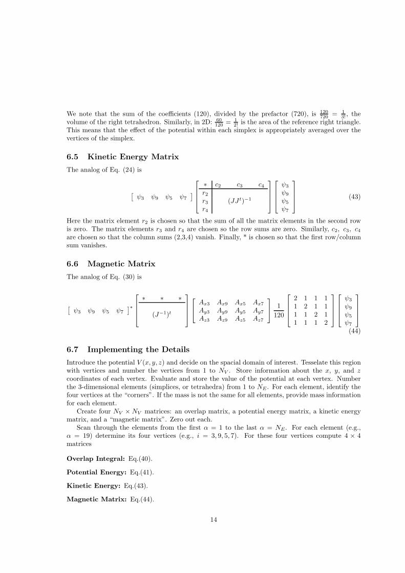
We note that the sum of the coefficients (120), divided by the prefactor (720), is 120

720= 1

3!, the

volume of the right tetrahedron. Similarly, in 2D: 60

120= 1

2!is the area of the reference right triangle.

This means that the effect of the potential within each simplex is appropriately averaged over thevertices of the simplex.

6.5 Kinetic Energy Matrix

The analog of Eq. (24) is

[

ψ3 ψ9 ψ5 ψ7

]

∗ c2 c3 c4r2r3 (JJ t)−1

r4

ψ3

ψ9

ψ5

ψ7

(43)

Here the matrix element r2 is chosen so that the sum of all the matrix elements in the second rowis zero. The matrix elements r3 and r4 are chosen so the row sums are zero. Similarly, c2, c3, c4are chosen so that the column sums (2,3,4) vanish. Finally, * is chosen so that the first row/columnsum vanishes.

6.6 Magnetic Matrix

The analog of Eq. (30) is

[

ψ3 ψ9 ψ5 ψ7

]∗

∗ ∗ ∗

(J−1)t

Ax3 Ax9 Ax5 Ax7

Ay3 Ay9 Ay5 Ay7

Az3 Az9 Az5 Az7

1

120

2 1 1 11 2 1 11 1 2 11 1 1 2

ψ3

ψ9

ψ5

ψ7

(44)

6.7 Implementing the Details

Introduce the potential V (x, y, z) and decide on the spacial domain of interest. Tesselate this regionwith vertices and number the vertices from 1 to NV . Store information about the x, y, and zcoordinates of each vertex. Evaluate and store the value of the potential at each vertex. Numberthe 3-dimensional elements (simplices, or tetrahedra) from 1 to NE . For each element, identify thefour vertices at the “corners”. If the mass is not the same for all elements, provide mass informationfor each element.

Create four NV ×NV matrices: an overlap matrix, a potential energy matrix, a kinetic energymatrix, and a “magnetic matrix”. Zero out each.

Scan through the elements from the first α = 1 to the last α = NE. For each element (e.g.,α = 19) determine its four vertices (e.g., i = 3, 9, 5, 7). For these four vertices compute 4 × 4matrices

Overlap Integral: Eq.(40).

Potential Energy: Eq.(41).

Kinetic Energy: Eq.(43).

Magnetic Matrix: Eq.(44).

14

Add the 16 matrix elements from Eq.(XX) into the appropriate places of the NV × NV overlapmatrix. Do the same for the other three matrices from Eq.(24), Eq.(XX), and Eq.(28). The resultingquadratic form in the unknown amplitudes must be stationary to satisfy the variational principle.This means that the generalized eigenvalue equation

〈i|(KE + PE +ME − E)|j〉〈j|ψ〉 = 0 (45)

must be solved. Here 〈i|∗|j〉 are the matrix elements of the kinetic energy, potential energy, magneticenergy, and overlap matrices, respectively, and the row and column indices identify nodes.

7 Quantum Mechanics in the Finite Element Representation

We have computed energy eigenvalues and wavefunctions using the finite element method. Thismethod is used to transform differential equations to matrix equations. In a sense this method canbe regarded as a change of basis procedure similar in spirit to the standard (Dirac) transformationtheory for Quantum Mechanics. As a result we can ask the usual basic questions: What are the basisfunctions? What is the matrix representative of the position operator? The momentum operator?Are commutation relations preserved? Is the matrix representative of x2 equal to the square of thematrix representative of x?

7.1 Basis Functions

The matrix elements of all the matrices constructed so far are indexed by an integer i, where ilabels the various vertices in the tesselation. We define a set of “basis” functions for our matrixrepresentation by |i〉, with a 1 : 1 correspondence between the vertices i and the basis functions |i〉.In the coordinate representation these functions are 〈x|i〉. These functions assume value 1 at vertexi and fall off linearly to zero at the other two vertices of each of the triangles sharing i as a vertex.

This set of Nv functions is nonorthogonal and incomplete. They cannot form a basis in the usualsense. They do form a basis set for the piecewise linear functions that are defined by their values atthe vertices i. These functions are continuous everywhere, linear in the interior of each element, andnot differentiable on the boundaries of the elements. When we call these functions basis functionswe mean specifically within the space of such linear functions.

Dirac’s representation of Quantum Theory uses orthonormal and complete sets of basis functions.The FEM representation therefore shares some of the properties of Dirac’s more familiar formulation,and lacks some of the others.

The most important function that we can construct from these functions is the matrix of overlapintegrals

Oij = 〈i|j〉 =

∫

〈i|x〉 dx 〈x|j〉 = Gij (46)

where 〈i|x〉 = 〈x|i〉∗ and Gij reminds us that these overlap integrals should be considered as thematrix elements of a metric tensor. The metric tensor is nonsingular, sparse, and real if the functions〈x|j〉 are real.

It is very useful to introduce an alternate basis defined by

|r〉 = |i〉(G−1/2)ir (47)

15

Although the metric tensor G is sparse its inverse G−1 is not; nor is G−1/2. This means that thecorresponding spatial basis states 〈x|r〉 = 〈x|i〉(G−1/2)ir are not nearly as localized as the originalbasis functions 〈x|i〉. We should create a picture to illustrate this.

These Nv new basis vectors are orthonormal:

〈r|s〉 = (G−1/2)ri〈i|j〉(G−1/2)js = (G−1/2)riGij(G−1/2)js = δrs (48)

The resolution of the identity is simple in terms of the new set of vectors:

I = |r〉〈r| → |i〉(G−1/2)ir(G−1/2)rj〈j| = |i〉(G−1)ij〈j| (49)

It is possible to find two matrix representations of an operator A: one in the original basis andone in the orthonormal basis. These are related by

〈r|A|s〉 = (G−1/2)ri〈i|A|j〉(G−1/2)js or A = G−1/2AG−1/2 (50)

The operator A can be reconstructed from its matrix elements. Starting from the orthonormal set,we have

A = |r〉Ars〈s| = |i〉(G−1/2)ir(G−1/2)rkAkl(G

−1/2)ls(G−1/2)sj〈j| = |i〉(G−1AG−1)ij〈j| (51)

Operator products are constructed as follows

AB = 〈r|AB|t〉 = 〈r|A|s〉〈s|B|t〉 = AB =(

G−1/2AG−1/2

)(

G−1/2BG−1/2

)

= G−1/2AG−1BG−1/2

(52)In a similar way the operator product AB can be expressed as follows:

AB = |i〉(G−1AG−1BG−1)ij〈j| (53)

Here the matrices A and B sandwiched between the G−1 are the matrices of the operators A andB with respect to the original nonorthogonal basis vectors.

The prescription for finding the matrix representation of an operator A is therefore:

1. Compute the matrix elements of the operator in the original basis.

2. Multiply on both sides by G−1.

3. A = |i〉(G−1AG−1)ij〈j|

It remains to see how good an approximation this is to the operator A. For example, isthe matrix representation of x2 well approximated by the suitable square of the matrixrepresentation of the operator x?

With these remarks in hand we turn now to the computation of the matrices representing severalimportant operators. These matrices will be computed with respect to the nonorthogonal basis set.These can be transformed to the matrices with respect to the orthonormal basis set as shown in Eq.(50).

16

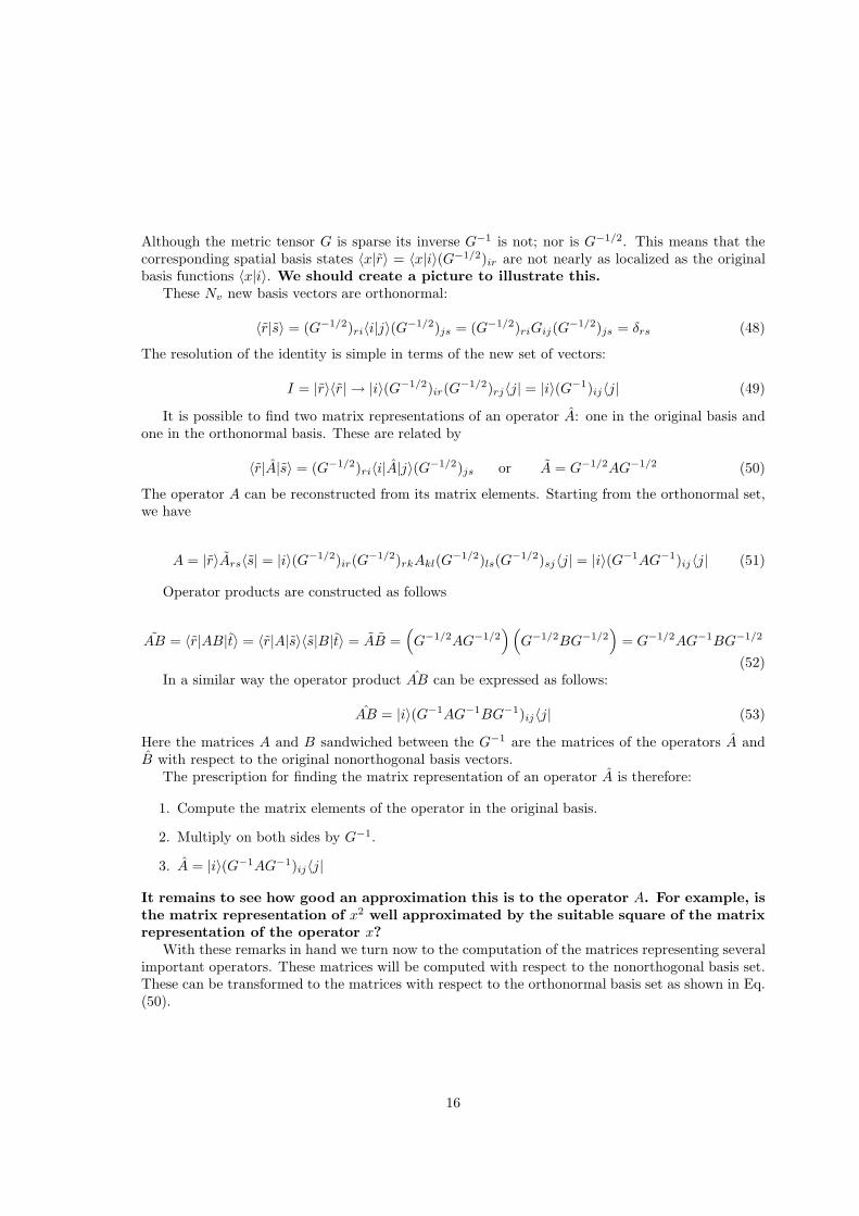
7.2 The Position Operator in the Linear FEM Basis

The matrix representation of the x coordinate of the position operator is built up in the usual fashionby carrying out the integral

∫

ψ19xψ19dx ∧ dy. We first express the x coordinate in terms of thecoordinates of points 3, 9, 5:

x = x3 + (x9 − x3)ξ + (x5 − x3)η = x3φ0 + x9φ1 + x5φ2 (54)

The integral over this triangle is

|J |∫ ∫

(ψ3φ0 + ψ9φ1 + ψ5φ2)2(x3φ0 + x9φ1 + x5φ2) dξ ∧ dη (55)

It is clear that the result involves integrals over products of three linear basis functions, which aregiven in Eq. (18). In fact, the result is evident by making a small change in Eq. (20):

|J |120

∣

∣

∣

∣

x9 − x3 y9 − y3x5 − x3 y5 − y3

∣

∣

∣

∣

×[

ψ3 ψ9 ψ5

]

6x3 + 2x9 + 2x5 2x3 + 2x9 + 1x5 2x3 + 1x9 + 2x5

2x3 + 2x9 + 1x5 2x3 + 6x9 + 2x5 1x3 + 2x9 + 2x5

2x3 + 1x9 + 2x5 1x3 + 2x9 + 2x5 2x3 + 2x9 + 6x5

ψ3

ψ9

ψ5

(56)It should be pointed out that the matrix representation of the first cordinate of the position operatorx = (x1, x2) = (x, y) depends on the y coordinates of the vertices in the tesselation through thevalue of the jacobian. Similar results hold for the matrix representation of the y coordinate. In theevent that the tesselation is regular (all simplices have the same measure) the matrix representationof the first coordinate x is independent of all y coordinates.

If it is necessary to use complex wavefunctions, the row vector on the left should be conjugated.Extensions to 3 dimensions are straightforward.

7.3 The Momentum Operator in the Linear FEM Basis

We compute the matrix representation of the gradient operator:

∫

ψ∗19

[

∂/∂x∂/∂y

]

ψ19 dx ∧ dy = |J |∫

(ψ3φ0 + ψ9φ1 + ψ5φ2)∗J−1

[

ψ9 − ψ3

ψ5 − ψ3

]

dξ ∧ dη (57)

We have used Eq. (22) to replace the action of the partial derivatives on the wavefunction by a columnvector of differences. The integral is linear in the basis functions. Further,

∫ ∫

φi(ξ, η)dξ ∧ dη = 1

6

for each of the basis functions. Putting this all together, we find

∫

ψ∗19

[

∂/∂x∂/∂y

]

ψ19 dx ∧ dy = |J | 1

6(ψ3 + ψ9 + ψ5)

∗

∗J−1

∗

ψ3

ψ9

ψ5

(58)

As before, the matrix elements * are chosen so that the row sums vanish.XXXXXXXXXXXXXXXXXXXXXXXXXXXXXXXXXXXX?? remove

7.4 Function Algebra

The basis functions |φi〉 can be used to represent functions that have known values at each vertex:f(x) →

∑

fiφi(x). Such functions form a linear vector space, and the functions φi(x) are a basis

17

set for the linear vector space of functions that are linear on each element. The column vectorscol(fi) represent these functions. Addition is simple: αf(x) + βg(x) → col(αfi + βgi). However,these vectors cannot be used to describe the composition properties f × g under multiplication.

To get around this problem we map each function to an operator: an Nv ×Nv diagonal matrixunder

f(x) →∑

fiφi(x) → col(fi) → f →∑

|r〉fr〈r| (59)

This is a diagonal matrix. Addition and multiplication are well-defined: ˆαf + βg = αf + βg andˆ(f ∗ g) = f × g. The matrix elements of the diagonal matrix representation of f are

〈i|f |j〉 = 〈i|r〉fr〈r|j〉 = (G1/2)irfr(G1/2)rj (60)

7.5 Operator Algebra

Suppose that we have two operators A and B. To construct a matrix representation of theseoperators with nice algebraic properties, we should be able to construct operators representing theirsum and their product from the matrix representations of the operators themselves.

Define Γ(A) to be the matrix representing the operator A in some finite element construction(i.e., a tesselation is specified, followed by specification of basis functions). Similarly: B → Γ(B).

It is intuitive that Γ(A+B) = Γ(A)+Γ(B); it is even easy to prove. It is not intuitive, even notcorrect, that Γ(A·B) = Γ(A)×Γ(B), where · means operator product and × is matrix multiplication.

Is there some way we can turn operator products into matrix multiplication of some type? Toget a sense of this, set B = I, where I is the identity operator. Then define

Γ(A) = Γ(A · I) = Γ(A) ⊗ Γ(I) = Γ(A) (61)

In this expression Γ(I) = O is the matrix of overlap integrals. If Eq. (51) is to be true as anidentity, then ⊗ = O−1. Elegantly: Γ(·) = O−1 = Γ−1(I). The conclusion is that we can representoperator products as matrix products by inserting the inverse of the overlap matrix between eachof the operators that we are taking the product of:

Γ(A · B) = Γ(A) × Γ(·) × Γ(B) = Γ(A) ×O−1 × Γ(B) (62)

In particular

Γ(KE) =~

2

2mΓ(∇)∗ ×O−1 × Γ(∇) (63)

It is necessary to check these assertions!!

xXXXXXXXXXXXXXXXXXXX ??? remove

7.6 Measure

Remark: One natural question that may come up is: What measure should we assign to eachvertex? In the natural linear basis, I have good arguments for the following response. ComputeM , the area/volume (measure) of the physical space that is being approximated. Determine the

trace of the overlap matrix computed before boundary conditions are applied: T =∑NV

i=1OLii. The

measure associated with vertex i is µ(i) = OLii × (M/T ). We need a ‘proof by picture’.

18

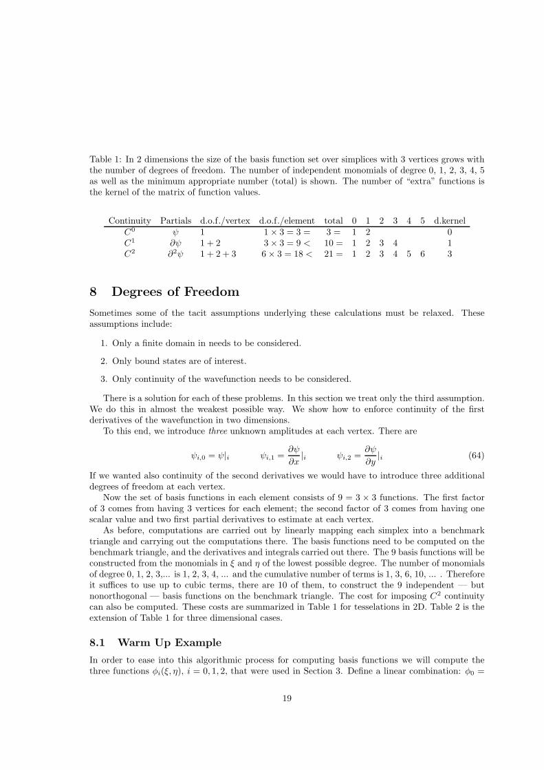
Table 1: In 2 dimensions the size of the basis function set over simplices with 3 vertices grows withthe number of degrees of freedom. The number of independent monomials of degree 0, 1, 2, 3, 4, 5as well as the minimum appropriate number (total) is shown. The number of “extra” functions isthe kernel of the matrix of function values.

Continuity Partials d.o.f./vertex d.o.f./element total 0 1 2 3 4 5 d.kernelC0 ψ 1 1 × 3 = 3 = 3 = 1 2 0C1 ∂ψ 1 + 2 3 × 3 = 9 < 10 = 1 2 3 4 1C2 ∂2ψ 1 + 2 + 3 6 × 3 = 18 < 21 = 1 2 3 4 5 6 3

8 Degrees of Freedom

Sometimes some of the tacit assumptions underlying these calculations must be relaxed. Theseassumptions include:

1. Only a finite domain in needs to be considered.

2. Only bound states are of interest.

3. Only continuity of the wavefunction needs to be considered.

There is a solution for each of these problems. In this section we treat only the third assumption.We do this in almost the weakest possible way. We show how to enforce continuity of the firstderivatives of the wavefunction in two dimensions.

To this end, we introduce three unknown amplitudes at each vertex. There are

ψi,0 = ψ|i ψi,1 =∂ψ

∂x|i ψi,2 =

∂ψ

∂y|i (64)

If we wanted also continuity of the second derivatives we would have to introduce three additionaldegrees of freedom at each vertex.

Now the set of basis functions in each element consists of 9 = 3 × 3 functions. The first factorof 3 comes from having 3 vertices for each element; the second factor of 3 comes from having onescalar value and two first partial derivatives to estimate at each vertex.

As before, computations are carried out by linearly mapping each simplex into a benchmarktriangle and carrying out the computations there. The basis functions need to be computed on thebenchmark triangle, and the derivatives and integrals carried out there. The 9 basis functions will beconstructed from the monomials in ξ and η of the lowest possible degree. The number of monomialsof degree 0, 1, 2, 3,... is 1, 2, 3, 4, ... and the cumulative number of terms is 1, 3, 6, 10, ... . Thereforeit suffices to use up to cubic terms, there are 10 of them, to construct the 9 independent — butnonorthogonal — basis functions on the benchmark triangle. The cost for imposing C2 continuitycan also be computed. These costs are summarized in Table 1 for tesselations in 2D. Table 2 is theextension of Table 1 for three dimensional cases.

8.1 Warm Up Example

In order to ease into this algorithmic process for computing basis functions we will compute thethree functions φi(ξ, η), i = 0, 1, 2, that were used in Section 3. Define a linear combination: φ0 =

19

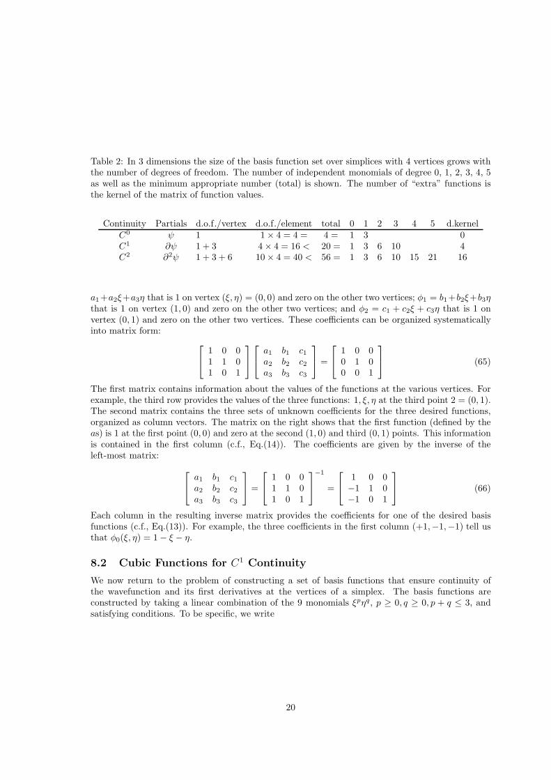
Table 2: In 3 dimensions the size of the basis function set over simplices with 4 vertices grows withthe number of degrees of freedom. The number of independent monomials of degree 0, 1, 2, 3, 4, 5as well as the minimum appropriate number (total) is shown. The number of “extra” functions isthe kernel of the matrix of function values.

Continuity Partials d.o.f./vertex d.o.f./element total 0 1 2 3 4 5 d.kernelC0 ψ 1 1 × 4 = 4 = 4 = 1 3 0C1 ∂ψ 1 + 3 4 × 4 = 16 < 20 = 1 3 6 10 4C2 ∂2ψ 1 + 3 + 6 10 × 4 = 40 < 56 = 1 3 6 10 15 21 16

a1+a2ξ+a3η that is 1 on vertex (ξ, η) = (0, 0) and zero on the other two vertices; φ1 = b1+b2ξ+b3ηthat is 1 on vertex (1, 0) and zero on the other two vertices; and φ2 = c1 + c2ξ + c3η that is 1 onvertex (0, 1) and zero on the other two vertices. These coefficients can be organized systematicallyinto matrix form:

1 0 01 1 01 0 1

a1 b1 c1a2 b2 c2a3 b3 c3

=

1 0 00 1 00 0 1

(65)

The first matrix contains information about the values of the functions at the various vertices. Forexample, the third row provides the values of the three functions: 1, ξ, η at the third point 2 = (0, 1).The second matrix contains the three sets of unknown coefficients for the three desired functions,organized as column vectors. The matrix on the right shows that the first function (defined by theas) is 1 at the first point (0, 0) and zero at the second (1, 0) and third (0, 1) points. This informationis contained in the first column (c.f., Eq.(14)). The coefficients are given by the inverse of theleft-most matrix:

a1 b1 c1a2 b2 c2a3 b3 c3

=

1 0 01 1 01 0 1

−1

=

1 0 0−1 1 0−1 0 1

(66)

Each column in the resulting inverse matrix provides the coefficients for one of the desired basisfunctions (c.f., Eq.(13)). For example, the three coefficients in the first column (+1,−1,−1) tell usthat φ0(ξ, η) = 1 − ξ − η.

8.2 Cubic Functions for C1 Continuity

We now return to the problem of constructing a set of basis functions that ensure continuity ofthe wavefunction and its first derivatives at the vertices of a simplex. The basis functions areconstructed by taking a linear combination of the 9 monomials ξpηq, p ≥ 0, q ≥ 0, p + q ≤ 3, andsatisfying conditions. To be specific, we write

20

φ =[

1 ξ η ξ2 ξη η2 ξ3 ξ2η1 ξ1η2 η3]

a0,0

a1,0

a0,1

a2,0

a1,1

a0,2

a3,0

a2,1

a1,2

a0,3

(67)

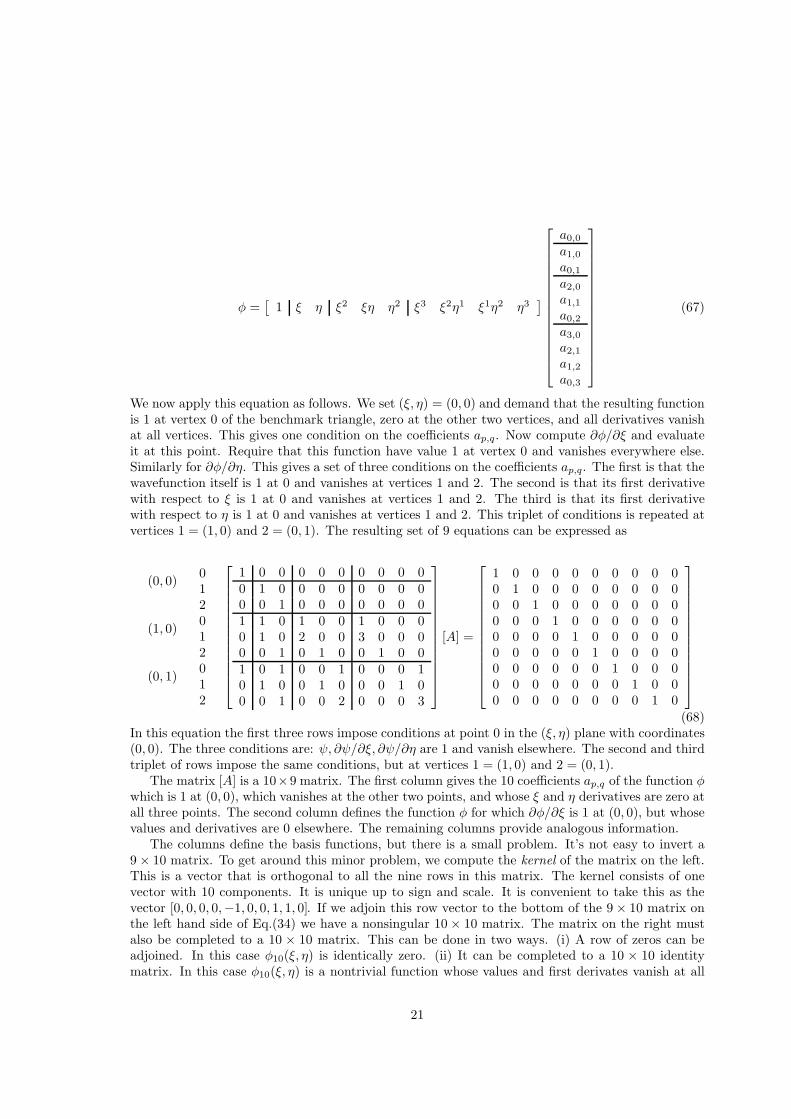
We now apply this equation as follows. We set (ξ, η) = (0, 0) and demand that the resulting functionis 1 at vertex 0 of the benchmark triangle, zero at the other two vertices, and all derivatives vanishat all vertices. This gives one condition on the coefficients ap,q. Now compute ∂φ/∂ξ and evaluateit at this point. Require that this function have value 1 at vertex 0 and vanishes everywhere else.Similarly for ∂φ/∂η. This gives a set of three conditions on the coefficients ap,q. The first is that thewavefunction itself is 1 at 0 and vanishes at vertices 1 and 2. The second is that its first derivativewith respect to ξ is 1 at 0 and vanishes at vertices 1 and 2. The third is that its first derivativewith respect to η is 1 at 0 and vanishes at vertices 1 and 2. This triplet of conditions is repeated atvertices 1 = (1, 0) and 2 = (0, 1). The resulting set of 9 equations can be expressed as

(0, 0)

(1, 0)

(0, 1)

012012012

1 0 0 0 0 0 0 0 0 00 1 0 0 0 0 0 0 0 00 0 1 0 0 0 0 0 0 01 1 0 1 0 0 1 0 0 00 1 0 2 0 0 3 0 0 00 0 1 0 1 0 0 1 0 01 0 1 0 0 1 0 0 0 10 1 0 0 1 0 0 0 1 00 0 1 0 0 2 0 0 0 3

[A] =

1 0 0 0 0 0 0 0 0 00 1 0 0 0 0 0 0 0 00 0 1 0 0 0 0 0 0 00 0 0 1 0 0 0 0 0 00 0 0 0 1 0 0 0 0 00 0 0 0 0 1 0 0 0 00 0 0 0 0 0 1 0 0 00 0 0 0 0 0 0 1 0 00 0 0 0 0 0 0 0 1 0

(68)In this equation the first three rows impose conditions at point 0 in the (ξ, η) plane with coordinates(0, 0). The three conditions are: ψ, ∂ψ/∂ξ, ∂ψ/∂η are 1 and vanish elsewhere. The second and thirdtriplet of rows impose the same conditions, but at vertices 1 = (1, 0) and 2 = (0, 1).

The matrix [A] is a 10×9 matrix. The first column gives the 10 coefficients ap,q of the function φwhich is 1 at (0, 0), which vanishes at the other two points, and whose ξ and η derivatives are zero atall three points. The second column defines the function φ for which ∂φ/∂ξ is 1 at (0, 0), but whosevalues and derivatives are 0 elsewhere. The remaining columns provide analogous information.

The columns define the basis functions, but there is a small problem. It’s not easy to invert a9 × 10 matrix. To get around this minor problem, we compute the kernel of the matrix on the left.This is a vector that is orthogonal to all the nine rows in this matrix. The kernel consists of onevector with 10 components. It is unique up to sign and scale. It is convenient to take this as thevector [0, 0, 0, 0,−1, 0, 0, 1, 1, 0]. If we adjoin this row vector to the bottom of the 9 × 10 matrix onthe left hand side of Eq.(34) we have a nonsingular 10 × 10 matrix. The matrix on the right mustalso be completed to a 10 × 10 matrix. This can be done in two ways. (i) A row of zeros can beadjoined. In this case φ10(ξ, η) is identically zero. (ii) It can be completed to a 10 × 10 identitymatrix. In this case φ10(ξ, η) is a nontrivial function whose values and first derivates vanish at all

21

three vertices. As a next step the 10× 10 matrix of coefficients [A] is solved for by matrix inversion.The three sets of three columns of [A] define functions φ with special properties at the three points0, 1, 2. This matrix is

1 0 0 0 0 0 0 0 0 00 1 0 0 0 0 0 0 0 00 0 1 0 0 0 0 0 0 0−3 −2 0 3 −1 0 0 0 0 00 −1/3 −1/3 0 0 1/3 0 1/3 0 −1/3−3 0 −2 0 0 0 3 0 −1 02 1 0 −2 1 0 0 0 0 00 1/3 −2/3 0 0 2/3 0 −1/3 0 1/30 −2/3 1/3 0 0 −1/3 0 2/3 0 1/32 0 1 0 0 0 −2 0 1 0

(69)

from which it is an easy matter to read off the nine basis functions for the benchmark triangle. Theyare:

φ1 = 1 − 3ξ2 − 3η2 + 2ξ3 + 2η3

φ2 = ξ − 2ξ2 + ξ3 + 1

3(−ξη + ξ2η − 2ξη2) = ξ − 2ξ2 + ξ3 − ξη2 + φ10

φ3 = η − 2η2 + η3 + 1

3(−ξη + ξη2 − 2ξ2η) = η − 2η2 + η3 − ηξ2 + φ10

φ4 = 3ξ2 − 2ξ3

φ5 = −ξ2 + ξ3

φ6 = 1

3(ξη + 2ξ2η − ξη2) = ξ2η − φ10

φ7 = 3η2 − 2η3

φ8 = 1

3(ξη + 2ξη2 − ξ2η) = η2ξ − φ10

φ9 = −η2 + η3

φ10 = 1

3(−ξη + ξη2 + ξ2η)

(70)

8.3 “Gauge” Freedom

The shape function φ10, as well as its derivatives with respect to both ξ and η, evaluates to 0 onthe three vertices. This functions behaves in the spirit of “gauge” transformations. The algebraicexpressions for the shape functions can be simplified by adding or subtracting φ10 to: φ2, φ3, φ6, φ8.We may/maynot make this transformation in our applications. Such simplification does not changethe nature of the symmetries described next.

8.4 Symmetries of the Cubic Functions

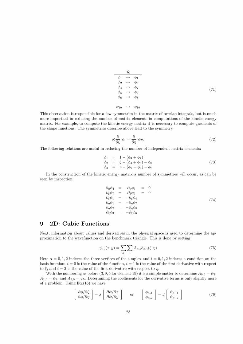
These shape functions exhibit the following symmetries under the reflection operation R that ex-changes ξ with η:

22

Rφ1 ↔ φ1

φ2 ↔ φ3

φ4 ↔ φ7

φ5 ↔ φ9

φ6 ↔ φ8

φ10 ↔ φ10

(71)

This observation is responsible for a few symmetries in the matrix of overlap integrals, but is muchmore important in reducing the number of matrix elements in computations of the kinetic energymatrix. For example, to compute the kinetic energy matrix it is necessary to compute gradients ofthe shape functions. The symmetries describe above lead to the symmetry

R ∂

∂ξφi =

∂

∂ηφRi (72)

The following relations are useful in reducing the number of independent matrix elements:

φ1 = 1 − (φ4 + φ7)φ2 = ξ − (φ4 + φ5) − φ8

φ3 = η − (φ7 + φ9) − φ6

(73)

In the construction of the kinetic energy matrix a number of symmetries will occur, as can beseen by inspection:

∂ηφ4 = ∂ηφ5 = 0∂ξφ7 = ∂ξφ9 = 0∂ξφ1 = −∂ξφ4

∂ηφ1 = −∂ηφ7

∂ηφ2 = −∂ηφ8

∂ξφ3 = −∂ξφ6

(74)

9 2D: Cubic Functions

Next, information about values and derivatives in the physical space is used to determine the ap-proximation to the wavefunction on the benchmark triangle. This is done by setting

ψ19(x, y) =∑

α

∑

i

Aα,iφα,i(ξ, η) (75)

Here α = 0, 1, 2 indexes the three vertices of the simplex and i = 0, 1, 2 indexes a condition on thebasis function: i = 0 is the value of the function, i = 1 is the value of the first derivative with respectto ξ, and i = 2 is the value of the first derivative with respect to η.

With the numbering as before (3, 9, 5 for element 19) it is a simple matter to determine A0,0 = ψ3,A1,0 = ψ9, and A2,0 = ψ5. Determining the coefficients for the derivative terms is only slightly moreof a problem. Using Eq.(16) we have

[

∂φ/∂ξ∂φ/∂η

]

= J

[

∂ψ/∂x∂ψ/∂y

]

or

[

φα,1

φα,2

]

= J

[

ψα′,1

ψα′,2

]

(76)

23

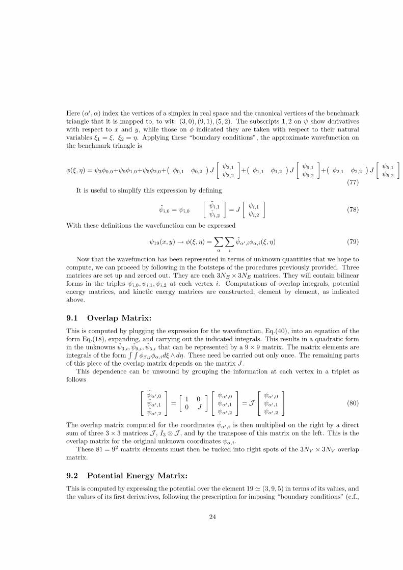
Here (α′, α) index the vertices of a simplex in real space and the canonical vertices of the benchmarktriangle that it is mapped to, to wit: (3, 0), (9, 1), (5, 2). The subscripts 1, 2 on ψ show derivativeswith respect to x and y, while those on φ indicated they are taken with respect to their naturalvariables ξ1 = ξ, ξ2 = η. Applying these “boundary conditions”, the approximate wavefunction onthe benchmark triangle is

φ(ξ, η) = ψ3φ0,0+ψ9φ1,0+ψ5φ2,0+(

φ0,1 φ0,2

)

J

[

ψ3,1

ψ3,2

]

+(

φ1,1 φ1,2

)

J

[

ψ9,1

ψ9,2

]

+(

φ2,1 φ2,2

)

J

[

ψ5,1

ψ5,2

]

(77)It is useful to simplify this expression by defining

ψi,0 = ψi,0

[

ψi,1

ψi,2

]

= J

[

ψi,1

ψi,2

]

(78)

With these definitions the wavefunction can be expressed

ψ19(x, y) → φ(ξ, η) =∑

α

∑

i

ψα′,iφα,i(ξ, η) (79)

Now that the wavefunction has been represented in terms of unknown quantities that we hope tocompute, we can proceed by following in the footsteps of the procedures previously provided. Threematrices are set up and zeroed out. They are each 3NE × 3NE matrices. They will contain bilinearforms in the triples ψi,0, ψi,1, ψi,2 at each vertex i. Computations of overlap integrals, potentialenergy matrices, and kinetic energy matrices are constructed, element by element, as indicatedabove.

9.1 Overlap Matrix:

This is computed by plugging the expression for the wavefunction, Eq.(40), into an equation of theform Eq.(18), expanding, and carrying out the indicated integrals. This results in a quadratic formin the unknowns ψ3,i, ψ9,i, ψ5,i that can be represented by a 9 × 9 matrix. The matrix elements areintegrals of the form

∫ ∫

φβ,jφα,idξ ∧ dη. These need be carried out only once. The remaining partsof this piece of the overlap matrix depends on the matrix J .

This dependence can be unwound by grouping the information at each vertex in a triplet asfollows

ψα′,0

ψα′,1

ψα′,2

=

[

1 00 J

]

ψα′,0

ψα′,1

ψα′,2

= J

ψα′,0

ψα′,1

ψα′,2

(80)

The overlap matrix computed for the coordinates ψα′,i is then multiplied on the right by a directsum of three 3 × 3 matrices J , I3 ⊗ J , and by the transpose of this matrix on the left. This is theoverlap matrix for the original unknown coordinates ψα,i.

These 81 = 92 matrix elements must then be tucked into right spots of the 3NV × 3NV overlapmatrix.

9.2 Potential Energy Matrix:

This is computed by expressing the potential over the element 19 ≃ (3, 9, 5) in terms of its values, andthe values of its first derivatives, following the prescription for imposing “boundary conditions” (c.f.,

24

Eqs.(38-40)). This expression, as well as a similar expression for the wavefunction (c.f., Eq.(40)), isplugged into an expression of the form Eq.(21) and the integrals over the variables ξ, η carried out.These integrals need be done only once. The result is once again a quadratic form in the unknowncoefficients ψ3,i, ψ9,i, ψ5,i. The matrix elements in the resulting 9 × 9 matrix are linear functions ofthe 9 pieces of information derived from the potential: its value at the three vertices and the valuesof its two first derivatives at these vertices: Vα,i. The result will have the look of Eq.(24), but thematrix will be much larger and the matrix elements more complicated.

The coefficients Vα,i within each matrix element must be transformed back to the known coor-dinates Vα,i by means of a transformation of the type in Eq.(41). The resulting potential energy

matrix, in the amplitudes ψα,i, must be transformed back to the matrix describing the quadraticform in the amplitudes ψα,i, as is done for the overlap matrix. This involves multiplying the matrixon the right by I3 ⊗ J and on the left by its transpose.

These 81 = 92 matrix elements must then be tucked into right spots of the 3NV × 3NV potentialenergy matrix.

9.3 Kinetic Energy Matrix:

The first step is the computation of the gradient of the wavefunction. We use Eq.(16) in the form∇xψ = J−1∇ξφ to make this computation more transparent. Specifically, we write ∂σ = (J−1)σ,µ∂µ

to abbreviate this relation, where 1 ≤ σ, ρ ≤ 2 are indices on the real space coordinates xσ =(x1, x2) = (x, y) and 1 ≤ µ, ν ≤ 2 are indices on the canonical coordinates ξµ = (ξ1, ξ2) = (ξ, η).With this shorthand (φβ,j,ν = ∂φβ,j/∂ξµ)

∂σψ → (J−1)σ,µφα,i,µψα′,i ∇ψ·∇ψ →∑

σ

ψβ′,j(J−1)σ,νφβ,j,ν(J−1)σ,µφα,i,µψα′,i (81)

The sum over σ is simply a matrix multiplication, leading to the symmetric matrix ((JJ t)−1)ν,µ.The integrals over the product of derivatives of the basis functions can be represented by somethingwith lots of indices. It is useful to represent this as a 2 × 2 matrix for the four triples (β, j;α, i):

M(β, j;α, i)ν,µ =

∫ ∫

φβ,j,νφα,i,µ dξ ∧ dη (82)

The quadratic form representing the kinetic energy is

~2

2mψβ′,j Tr

(

M(β, j;α, i)(JJ t)−1)

ψα′,i (83)

The trace is over 2 × 2 matrices. In order to construct the quadratic form in the original set ofunknown coordinates ψα′,i this 9 × 9 matrix must be multiplied on the right by I3 ⊗ J and on theleft by its transpose, as usual.

Remind myself to study the symmetry of the integrals in Eq.(43) ASAP.These 81 = 92 matrix elements must then be tucked into right spots of the 3NV × 3NV kinetic

energy matrix.The details are implemented exactly as in Sect. 3.5. There results an equation of the form

of Eq.(3.9). The only difference now is that the index i for vertices in Eq.(3.9) is replaced by adouble index i, r, where the first index labels the individual vertices 1 ≤ i, j ≤ NV and the secondindex 0 ≤ r, s ≤ 2 labels the conditions, continuity of the wavefunction, continuity of the two firstderivatives, at that vertex. Once again, the equation

〈i, r|(KE + PE − E)|j, s〉〈j, s|ψ〉 = 0 (84)

25

Table 3: Cubic basis functions for a right tetrahedron with vertices at (0,0,0) and the triples (1,0,0),(0,1,0), and (0,0,1).

(0, 0, 0) (1, 0, 0) (0, 1, 0) (0, 0, 1)φ1 = 1 − φ5 − φ9 − φ13 φ5 = 3ξ2 − 2ξ3 φ9 = 3η2 − 2η3 φ13 = 3ζ2 − 2ζ3

φ2 = ξ − 2ξ2 + ξ3 − ξ(η2 + ζ2) φ6 = −ξ2 + ξ3 φ10 = η2ξ φ14 = ζ2ξφ2 = η − 2η2 + η3 − η(ζ2 + ξ2) φ7 = ξ2η φ11 = −η2 + η3 φ15 = ζ2ηφ4 = ζ − 2ζ2 + ζ3 − ζ(ξ2 + η2) φ8 = ξ2ζ φ12 = η2ζ φ16 = −ζ2 + ζ3

(85)

is to be diagonalized and the eigenvectors given the usual tests for convergence to something mean-ingful.

10 3D: Cubic Functions

10.1 Basis functions

The cubic basis functions for four nodes with four degrees of freedom are:The remaining four functions φ17 − φ20 fall into two groups: φ∗ = − 1

3xixj + 2

3(x2

i xj + x2jxi)

(1 ≤ i 6= j ≤ 3) and φ20 = ξηζ.Remark: There are lots of symmetries among these functions and their derivatives. This

means that the number of independent integrals in the overlap, potential, and kinetic matricesis correspondingly reduced.

11 Summary

In finite-**** methods the wavefunction is approximated by its (unknown) values at a whole bunch(NV ) of closely spaced vertices. The approximation is specified by a set of functions, linearly scaledby the values of the wavefunctions at the vertices. When these representations for the wavefunctionare substituted into the action integral, then the appropriate actions can be carried out on the basisset of functions, and then the integrals can be carried out. The result is a bilinear expression in termsof the unknown values at each vertex and their complex conjugates. This expression can be rewrittenin matrix form. In this form the matrix that represents the Action Integral is an NV ×NV hermitianmatrix. When the physics allows the wave function to be real (e.g., bound states), the unknowncomponents are real, the Action Integral is represented by a quadratic form in this unknown valuesof the wave function, and we have a real symmetric NV ×NV matrix to diagonalize. It’s eigenvaluesapproximate the bound states and its eigenvectors determine the values of the different eigenmodesat the various vertices.

12 Appendix A: Wavefunctions on Surfaces

Two-dimensional regions on which we compute wavefunctions need not be flat. The simplest two-dimensional surface on which to compute solutions of the Schrodinger equation is the sphere S2: thesurface x2 + y2 + z2 = 1 in R3. The solutions are already known: they are the spherical harmonicsY l

m(θ, φ).

26

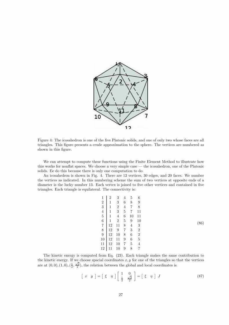
Figure 4: The icosahedron is one of the five Platonic solids, and one of only two whose faces are alltriangles. This figure presents a crude approximation to the sphere. The vertices are numbered asshown in this figure.

We can attempt to compute these functions using the Finite Element Method to illustrate howthis works for nonflat spaces. We choose a very simple case — the icosahedron, one of the Platonicsolids. Ee do this because there is only one computation to do.

An icosahedron is shown in Fig. 4. There are 12 vertices, 30 edges, and 20 faces. We numberthe vertices as indicated. In this numbering scheme the sum of two vertices at opposite ends of adiameter is the lucky number 13. Each vertex is joined to five other vertices and contained in fivetriangles. Each triangle is equilateral. The connectivity is:

1 2 3 4 5 62 1 3 6 8 93 1 2 4 7 84 1 3 5 7 115 1 4 6 10 116 1 2 5 9 107 12 11 8 4 38 12 9 7 3 29 12 10 8 6 210 12 11 9 6 511 12 10 7 5 412 11 10 9 8 7

(86)

The kinetic energy is computed from Eq. (23). Each triangle makes the same contribution tothe kinetic energy. If we choose spacial coordinates x, y for one of the triangles so that the vertices

are at (0, 0), (1, 0), (1

2,√

3

2), the relation between the global and local coordinates is

[

x y]

=[

ξ η]

[

1 01

2

√3

2

]

=[

ξ η]

J (87)

27

From this we compute

(J−1)t(J−1) = (JJ t)−1 =

[

4

3− 2

3

− 2

3

4

3

]

(88)

Using this result in Eq.(24) we find for the contribution to the Kinetic Energy matrix

2

3

2 −1 −1−1 2 −1−1 −1 2

(89)

Construction of the 12 × 12 kinetic energy matrix is now a piece of cake. It is

2 × 2

3

5 −1 −1 −1 −1 −1 0 0 0 0 0 0−1 5 −1 0 0 −1 0 −1 −1 0 0 0−1 −1 5 −1 0 0 −1 −1 0 0 0 0−1 0 −1 5 −1 0 −1 0 0 0 −1 0−1 0 0 −1 5 −1 0 0 0 −1 −1 0−1 −1 0 0 −1 5 0 0 −1 −1 0 00 0 −1 −1 0 0 5 −1 0 0 −1 −10 −1 −1 0 0 0 −1 5 −1 0 0 −10 −1 0 0 0 −1 0 −1 5 −1 0 −10 0 0 0 −1 −1 0 0 −1 5 −1 −10 0 0 −1 −1 0 −1 0 0 −1 5 −10 0 0 0 0 0 −1 −1 −1 −1 −1 5

(90)

For example, the sixth row is obtained as follows. The vertex 6 is contained in five triangles, soplace 5 × 2 × 2

3in the (6, 6) position in this matrix. The vertices connected to vertex 6 in triangles

are (1, 2, 5, 9, 10) (each of these vertices is in 2 triangles), so place 1 × 2 × −2

3in these columns in

the row 6 of this matrix. The common factor 4

3has been factored out of this matrix. All rows are

computed similarly.This real symmetric matrix has eigenvalues 0, 5±

√5, 6. The eigenvalue 0 is immediate: the sum

of the elements in each row is zero, so one eigenvector is the Goldstone mode (all components of theeigenvector are equal). This eigenvalue is nondegenerate and corresponds to the l = 0 S state. Theeigenvalue 5 −

√5 is triply degenerate, and corresponds to the l = 1 P state. The eigenvalue 6 is

5-fold degenerate and corresponds to the l = 2 D state. There are three (12 − 1 − 3 − 5) remaineigenvalues, all are 5 +

√5 that don’t coorrespond to any angular momentum states, since we have

truncated the discretization to too small (12) a number of vertices.

28

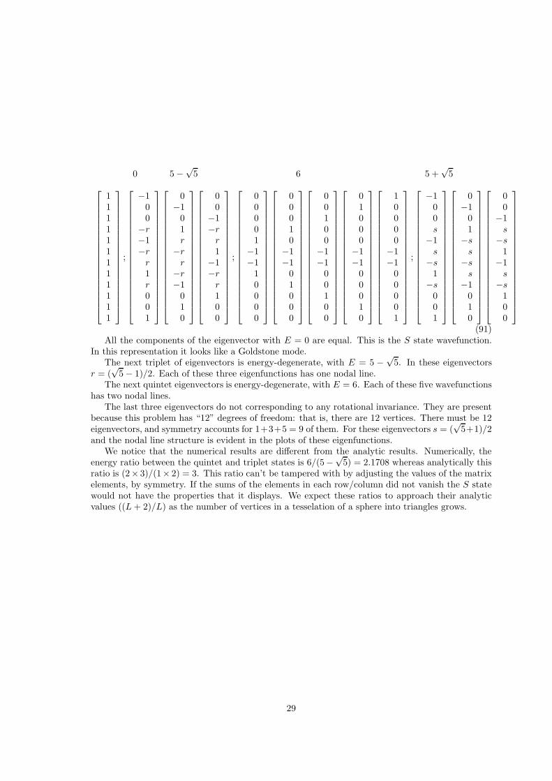
0 5 −√

5 6 5 +√

5

111111111111

;

−100

−r−1−rr1r001

0−1

01r

−rr

−r−1

010

00

−1−rr1

−1−rr100

;

00001

−1−1

10000

00010

−1−1

01000

00100

−1−1

00100

01000

−1−1

00010

10000

−1−1

00001

;

−100s

−1s

−s1

−s001

0−1

01

−ss

−ss

−1010

00

−1s

−s1

−1s

−s100

(91)All the components of the eigenvector with E = 0 are equal. This is the S state wavefunction.

In this representation it looks like a Goldstone mode.The next triplet of eigenvectors is energy-degenerate, with E = 5 −

√5. In these eigenvectors

r = (√

5 − 1)/2. Each of these three eigenfunctions has one nodal line.The next quintet eigenvectors is energy-degenerate, with E = 6. Each of these five wavefunctions

has two nodal lines.The last three eigenvectors do not corresponding to any rotational invariance. They are present

because this problem has “12” degrees of freedom: that is, there are 12 vertices. There must be 12eigenvectors, and symmetry accounts for 1+3+5 = 9 of them. For these eigenvectors s = (

√5+1)/2

and the nodal line structure is evident in the plots of these eigenfunctions.We notice that the numerical results are different from the analytic results. Numerically, the

energy ratio between the quintet and triplet states is 6/(5−√

5) = 2.1708 whereas analytically thisratio is (2× 3)/(1× 2) = 3. This ratio can’t be tampered with by adjusting the values of the matrixelements, by symmetry. If the sums of the elements in each row/column did not vanish the S statewould not have the properties that it displays. We expect these ratios to approach their analyticvalues ((L+ 2)/L) as the number of vertices in a tesselation of a sphere into triangles grows.

29