From Navier-Stokes to Saint-Venant - Inria · Presentation Derivation of Saint-Venant From...

Presentation Derivation of Saint-Venant

From Navier-Stokes to Saint-VenantCourse 1

E. Godlewski1 & J. Sainte-Marie1

1ANGE team

LJLL - January 2017


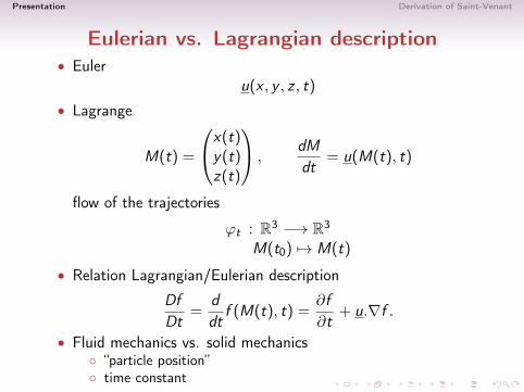
Eulerian vs. Lagrangian description• Euler

u(x , y , z , t)

• Lagrange

M(t) =

x(t)y(t)z(t)

,dMdt

= u(M(t), t)

flow of the trajectories

ϕt : R3 −→ R3

M(t0) 7→ M(t)

• Relation Lagrangian/Eulerian description

DfDt

=ddt

f (M(t), t) =∂f∂t

+ u.∇f .

• Fluid mechanics vs. solid mechanics◦ “particle position”◦ time constant


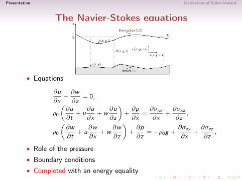
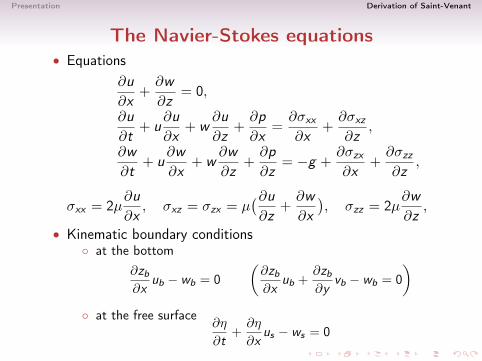
The Navier-Stokes equations

• Equations

∂u∂x

+∂w∂z

= 0,

ρ0

(∂u∂t

+ u∂u∂x

+ w∂u∂z

)+∂p∂x

=∂σxx

∂x+∂σxz

∂z,

ρ0

(∂w∂t

+ u∂w∂x

+ w∂w∂z

)+∂p∂z

= −ρ0g +∂σzx

∂x+∂σzz

∂z,

• Role of the pressure• Boundary conditions• Completed with an energy equality


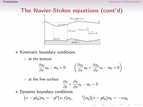
The Navier-Stokes equations (cont’d)

• Kinematic boundary conditions

◦ at the bottom∂zb

∂xub − wb = 0

(∂zb

∂xub +

∂zb

∂yvb − wb = 0

)◦ at the free surface

∂η

∂t+∂η

∂xus − ws = 0

• Dynamic boundary conditions(σ − pId )ns = −pa(x , t)ns ,

t(nb)(σ − pId )nb = −κub


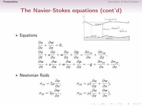
The Navier-Stokes equations (cont’d)

• Equations

∂u∂x

+∂w∂z

= 0,

∂u∂t

+ u∂u∂x

+ w∂u∂z

+∂p∂x

=∂σxx

∂x+∂σxz

∂z,

∂w∂t

+ u∂w∂x

+ w∂w∂z

+∂p∂z

= −g +∂σzx

∂x+∂σzz

∂z,

• Newtonian fluids

σxx = 2µ∂u∂x, σxz = µ

(∂u∂z

+∂w∂x),

σzz = 2µ∂w∂z

, σzx = µ(∂u∂z

+∂w∂x),


The Euler system• Equations

∂u∂x

+∂w∂z

= 0,

∂u∂t

+ u∂u∂x

+ w∂u∂z

+∂p∂x

= 0,

∂w∂t

+ u∂w∂x

+ w∂w∂z

+∂p∂z

= −g ,

• Boundary conditions◦ kinematic (bottom + free surface), dynamical (ps = pa)

• Energy equality: a constraint

∂

∂t

ˆ η

zb

E dz +∂

∂x

ˆ η

zb

u (E + p) dz = 0

withE =

u2 + w2

2+ gz

• The Euler system and physical solutions ?


Origins of the Euler/NS system• Mass within a volume V

m =

˚Vρdv

• Mass conservationdmdt

=

˚V

∂ρ

∂tdv +

‹Sρu.ds = 0

• Green-Ostrogradsky formula‹Sρu.ds =

˚Vdiv (ρu)dv

• local mass conservation equation

∂ρ

∂t+∂(ρu)

∂x+∂(ρv)

∂y+∂(ρw)

∂z= 0

• When ρ = cst∂u∂x

+∂v∂y

+∂w∂z

= 0


Origins of the Euler/NS system (cont’d)• Divergence free condition

∂u∂x

+∂v∂y

+∂w∂z

= 0

• Variation of velocity

du = u(x + udt, y + vdt, z + wdt)− u(x , y , z , t)

i.e.du =

∂u∂x

udt +∂u∂y

vdt +∂u∂z

wdt +∂u∂t

dt

• Acceleration a defined by du = adt

a =∂u∂t

+ u∂u∂x

+ v∂u∂y

+ w∂u∂z

• Fundamental law of dynamics

ρa− div (σT ) = −ρg

with σT = −pId + σ


Models for compressible fluids

• Euler equation (compressible gas dynamics)

∂ρ

∂x+∂(ρu)

∂x+∂(ρw)

∂z= 0,

∂(ρu)

∂t+∂(ρu2)

∂x+∂(ρuw)

∂z+∂p∂x

= 0,

∂(ρw)

∂t+∂(ρuw)

∂x+∂(ρw2)

∂z+∂p∂z

= 0,

∂E∂t

+∂u(E + p)

∂x+∂w(E + p)

∂z= 0,

with p = (γ − 1)ρe (for polytropic gas 1 ≤ γ ≤ 3) and

E =12ρ(u2 + w2) + ρe,

• Compressible ↔ incompressible : singular limit


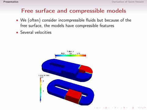
Free surface and compressible models• We (often) consider incompressible fluids but because of thefree surface, the models have compressible features

• Several velocities


Fluids with complex rheology• Newtonian fluids

σv ,xx = 2µ∂u∂x, σv ,xz = µ

(∂u∂z

+∂w∂x),

σv ,zz = 2µ∂w∂z

, σv ,zx = µ(∂u∂z

+∂w∂x),

• The Mohr-Coulomb criterion

σT = σN tan(φ) + c

c : cohesion, φ: internal friction angle• The Drucker-Prager criterion{

σ = σv + κ σv‖σv‖ if ‖σv‖ 6= 0,

‖σ‖ ≤ κ else

with κ =√2λ[p]+

• Also Herschel-Bulkley fluid,. . .


The Navier-Stokes equations• Equations

∂u∂x

+∂w∂z

= 0,

∂u∂t

+ u∂u∂x

+ w∂u∂z

+∂p∂x

=∂σxx

∂x+∂σxz

∂z,

∂w∂t

+ u∂w∂x

+ w∂w∂z

+∂p∂z

= −g +∂σzx

∂x+∂σzz

∂z,

σxx = 2µ∂u∂x, σxz = σzx = µ

(∂u∂z

+∂w∂x), σzz = 2µ

∂w∂z

,

• Kinematic boundary conditions◦ at the bottom

∂zb

∂xub − wb = 0

(∂zb

∂xub +

∂zb

∂yvb − wb = 0

)◦ at the free surface

∂η

∂t+∂η

∂xus − ws = 0

• Dynamic boundary conditions(σ − pId)ns = −pa(x , t)ns ,

t(nb)(σ − pId)nb = −κub


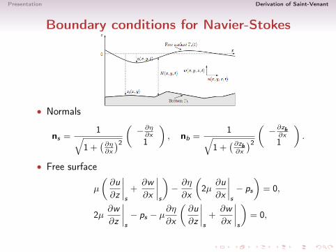
Boundary conditions for Navier-Stokes

• Normals

ns =1√

1 +(∂η∂x

)2(−∂η∂x1

), nb =

1√1 +

(∂zb∂x

)2(−∂zb∂x1

).

• Free surface

µ

(∂u∂z

∣∣∣∣s

+∂w∂x

∣∣∣∣s

)− ∂η

∂x

(2µ

∂u∂x

∣∣∣∣s− ps

)= 0,

2µ∂w∂z

∣∣∣∣s− ps − µ

∂η

∂x

(∂u∂z

∣∣∣∣s

+∂w∂x

∣∣∣∣s

)= 0,


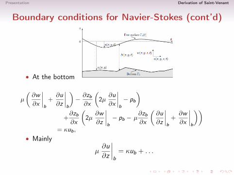
Boundary conditions for Navier-Stokes (cont’d)

• At the bottom

µ

(∂w∂x

∣∣∣∣b

+∂u∂z

∣∣∣∣b

)− ∂zb

∂x

(2µ

∂u∂x

∣∣∣∣b− pb

)+∂zb

∂x

(2µ

∂w∂z

∣∣∣∣b− pb − µ

∂zb

∂x

(∂u∂z

∣∣∣∣b

+∂w∂x

∣∣∣∣b

))= κub,

• Mainly

µ∂u∂z

∣∣∣∣b

= κub + . . .


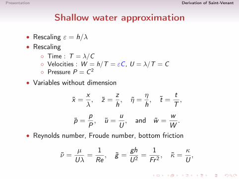
Shallow water approximation

• Rescaling ε = h/λ• Rescaling

◦ Time : T = λ/C◦ Velocities : W = h/T = εC , U = λ/T = C◦ Pressure P = C 2

• Variables without dimension

x =xλ, z =

zh, η =

η

h, t =

tT,

p =pP, u =

uU, and w =

wW.

• Reynolds number, Froude number, bottom friction

ν =µ

Uλ=

1Re, g =

ghU2 =

1Fr2 , κ =

κ

U,


Shallow water approximation (cont’d)

• Dimensionless 2D Navier-Stokes equations

∂u∂x

+∂w∂z

= 0

∂u∂ t

+∂u2

∂x+∂uw∂z

+∂p∂x

=∂

∂x

(2ν∂u∂x

)+∂

∂z

(ν

ε2∂u∂z

+ ν∂w∂x

)ε2(∂w∂ t

+∂uw∂x

+∂w2

∂z

)+∂p∂z

= −1 +∂

∂x

(ν∂u∂z

+ ε2ν∂w∂x

)+∂

∂z

(2ν∂w∂z

)• Boundary conditions

◦ kinematic (not modified)


Shallow water approximation (cont’d)

• Boundary conditions

◦ at the free surface

ν

ε

(∂u∂z

∣∣∣∣s

+ ε2∂w∂x

∣∣∣∣s

)− ε∂η

∂x

(2ν

∂u∂x

∣∣∣∣s− ps

)= 0,

2ν∂w∂z

∣∣∣∣s− ps − εν

∂η

∂x

(∂u∂z

∣∣∣∣s

+ ε2∂w∂x

∣∣∣∣s

)= 0,

• at the bottom

ν

ε

(ε2

∂w∂x

∣∣∣∣b

+∂u∂z

∣∣∣∣b

)− ε∂zb

∂x

(2ν

∂u∂x

∣∣∣∣b− pb

)+ε

∂zb

∂x

(2ν

∂w∂z

∣∣∣∣b− pb − ν

∂zb

∂x

(∂u∂z

∣∣∣∣b

+ ε2∂w∂x

∣∣∣∣b

))= κub,


Hydrostatic Navier-Stokes system

• With initial variables

∂u∂x

+∂w∂z

= 0

∂u∂t

+∂u2

∂x+∂uw∂z

+∂p∂x

=∂

∂x

(2ν∂u∂x

)+

∂

∂z

(ν∂u∂z

+ ν∂w∂x

)∂p∂z

= −g +∂

∂x

(ν∂u∂z

+ ν∂w∂x

)+

∂

∂z

(2ν∂w∂z

)• “A good model”• Simplified role of the pressure• Rather complex to analyse and solve


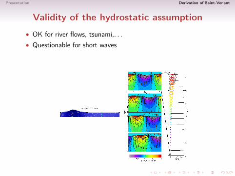
Validity of the hydrostatic assumption

• OK for river flows, tsunami,. . .• Questionable for short waves


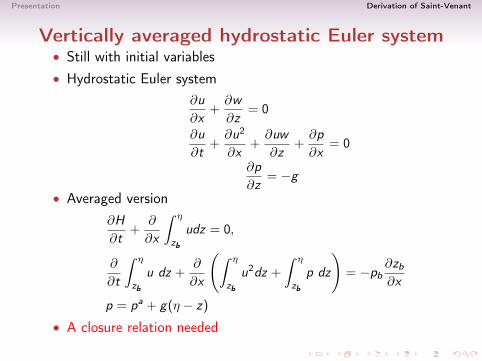
Vertically averaged hydrostatic Euler system• Still with initial variables• Hydrostatic Euler system

∂u∂x

+∂w∂z

= 0

∂u∂t

+∂u2

∂x+∂uw∂z

+∂p∂x

= 0

∂p∂z

= −g

• Averaged version∂H∂t

+∂

∂x

ˆ η

zb

udz = 0,

∂

∂t

ˆ η

zb

u dz +∂

∂x

(ˆ η

zb

u2dz +

ˆ η

zb

p dz

)= −pb

∂zb

∂x

p = pa + g(η − z)

• A closure relation needed


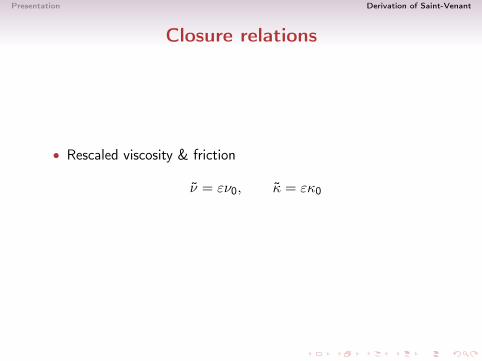
Closure relations

• Rescaled viscosity & friction

ν = εν0, κ = εκ0


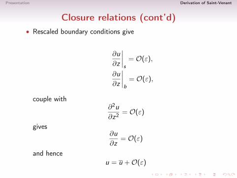
Closure relations (cont’d)• Rescaled boundary conditions give

∂u∂z

∣∣∣∣s

= O(ε),

∂u∂z

∣∣∣∣b

= O(ε),

couple with∂2u∂z2 = O(ε)

gives∂u∂z

= O(ε)

and henceu = u +O(ε)


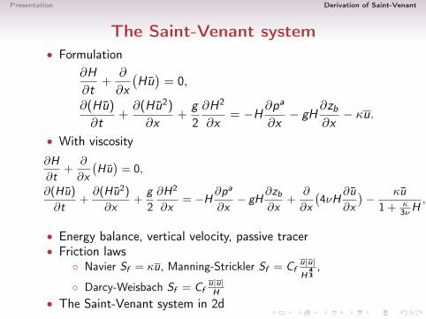
The Saint-Venant system• Formulation

∂H∂t

+∂

∂x(Hu)

= 0,

∂(Hu)

∂t+∂(Hu2)

∂x+

g2∂H2

∂x= −H

∂pa

∂x− gH

∂zb

∂x− κu.

• With viscosity∂H∂t

+∂

∂x(Hu)

= 0,

∂(Hu)

∂t+∂(Hu2)

∂x+

g2∂H2

∂x= −H

∂pa

∂x− gH

∂zb

∂x+

∂

∂x(4νH

∂u∂x)− κu

1 + κ3νH

,

• Energy balance, vertical velocity, passive tracer• Friction laws

◦ Navier Sf = κu, Manning-Strickler Sf = Cfu|u|H

43,

◦ Darcy-Weisbach Sf = Cfu|u|H

• The Saint-Venant system in 2d

From Navier-Stokes to Saint-Venant - Inria · Presentation Derivation of Saint-Venant From...

Documents

Transcript of From Navier-Stokes to Saint-Venant - Inria · Presentation Derivation of Saint-Venant From...