The Distribution of FApplied Statistics and Experimental Design Fritz Scholz — Fall 2006

It can be shown that

F =SSTreat/(t−1)SSE/(N− t)

∼ Ft−1,N−t,λ a noncentral F-distribution

with t−1 and N− t degrees of freedom and noncentrality parameter

λ = ∑ti=1 ni(µi− µ)2/σ2 = ∑

ti=1 ∑

nij=1(µi− µ)2/σ2

Under H0 : µ1 = . . . = µt this becomes the (central) Ft−1,N−t distribution.

We reject H0 whenever F ≥ Ft−1,N−t(1−α) = Fcrit = qf(1−α,t−1,N−t)

which denotes the (1−α)-quantile of the Ft−1,N−t distribution.

Power function: β(λ) = P(F ≥ Ft−1,N−t(1−α)) = 1−pf(Fcrit,t−1,N−t,λ)

1

Discussion of Noncentrality Parameter λApplied Statistics and Experimental Design Fritz Scholz — Fall 2006

The power of the ANOVA F-test is a monotone increasing function of

λ = ∑ti=1 ni(µi− µ)2/σ2 = N×∑

ti=1(ni/N)(µi− µ)2/σ2 = N×σ2

µ/σ2

= N×between treatment variation/within treatment variation

Thus we consider the drivers in λ.

λ increases as σ decreases (provided the µi are not all the same).

The more difference there is between the treatment means µi the higher λ

Increasing the sample sizes will magnify ni(µi− µ)2 (provided µ is stable).

The sample sizes we can plan for.

Later: we can reduce σ by blocking units into more homogeneous groups.

2

Optimal Allocation of Sample Sizes?Applied Statistics and Experimental Design Fritz Scholz — Fall 2006

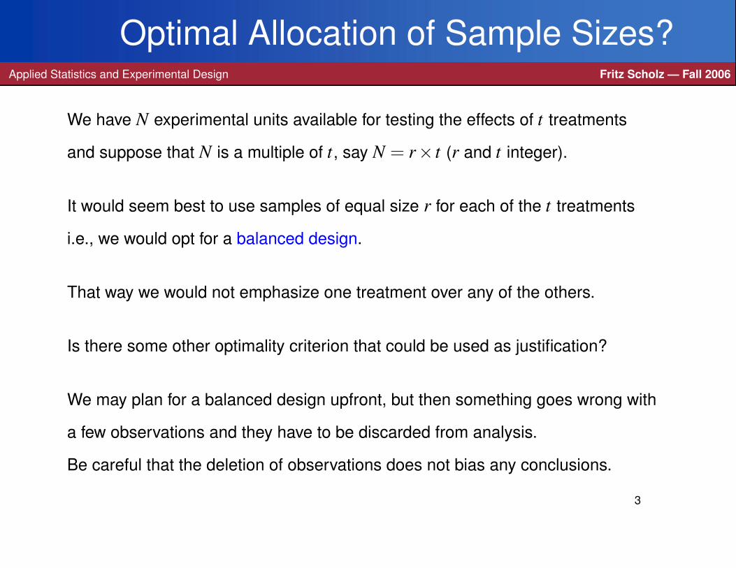
We have N experimental units available for testing the effects of t treatments

and suppose that N is a multiple of t, say N = r× t (r and t integer).

It would seem best to use samples of equal size r for each of the t treatments

i.e., we would opt for a balanced design.

That way we would not emphasize one treatment over any of the others.

Is there some other optimality criterion that could be used as justification?

We may plan for a balanced design upfront, but then something goes wrong with

a few observations and they have to be discarded from analysis.

Be careful that the deletion of observations does not bias any conclusions.

3

A Sample Size Allocation RationaleApplied Statistics and Experimental Design Fritz Scholz — Fall 2006

We may be concerned with alternatives where all means but one are the same.

Since we won’t know upfront which mean sticks out, we would want to maximize

the minimum power against all such contingencies. Max-Min Strategy!

If µ1 = µ+∆ and µ2 = . . . = µt = µ then µ = µ+n1∆/N and (algebra)

λ1 =t

∑i=1

ni(µi− µ)2/σ2 =

N∆2

σ2n1N

(1− n1

N

)and similarly λi =

N∆2

σ2niN

(1− ni

N

)for the other cases. It is easy to see now that for fixed σ

maxn1,...,nt

min1≤i≤t

[N∆2

σ2niN

(1− ni

N

)]is achieved when n1 = . . . = nt . That is because

niN

(1− ni

N

)increases for ni/N ≤ 1/2.

4

Using sample.sizeANOVA (see web page)Applied Statistics and Experimental Design Fritz Scholz — Fall 2006

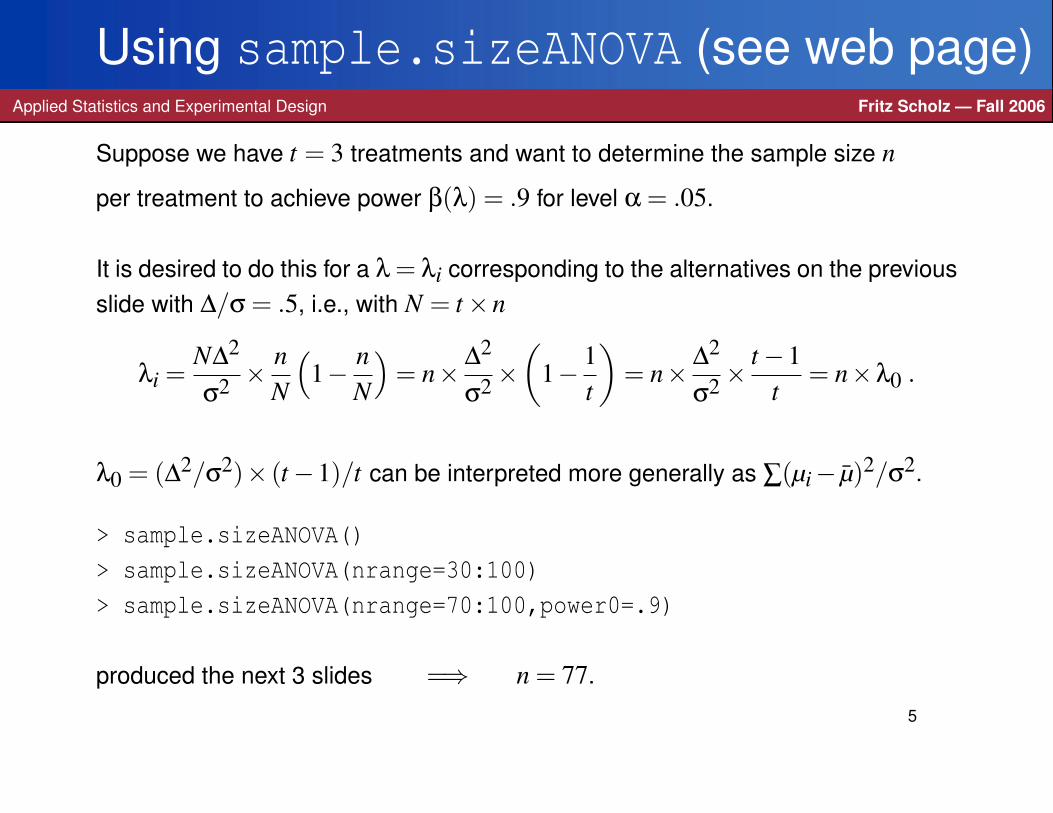
Suppose we have t = 3 treatments and want to determine the sample size n

per treatment to achieve power β(λ) = .9 for level α = .05.

It is desired to do this for a λ = λi corresponding to the alternatives on the previousslide with ∆/σ = .5, i.e., with N = t×n

λi =N∆2

σ2 × nN

(1− n

N

)= n× ∆2

σ2×(

1− 1t

)= n× ∆2

σ2×t−1

t= n×λ0 .

λ0 = (∆2/σ2)× (t−1)/t can be interpreted more generally as ∑(µi− µ)2/σ2.

> sample.sizeANOVA()

> sample.sizeANOVA(nrange=30:100)

> sample.sizeANOVA(nrange=70:100,power0=.9)

produced the next 3 slides =⇒ n = 77.

5

sample.sizeANOVA IApplied Statistics and Experimental Design Fritz Scholz — Fall 2006

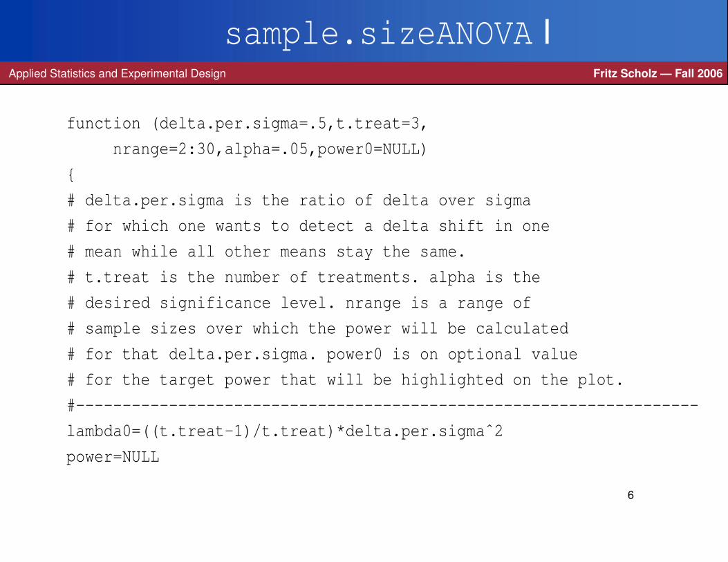
function (delta.per.sigma=.5,t.treat=3,

nrange=2:30,alpha=.05,power0=NULL)

{

# delta.per.sigma is the ratio of delta over sigma

# for which one wants to detect a delta shift in one

# mean while all other means stay the same.

# t.treat is the number of treatments. alpha is the

# desired significance level. nrange is a range of

# sample sizes over which the power will be calculated

# for that delta.per.sigma. power0 is on optional value

# for the target power that will be highlighted on the plot.

#-------------------------------------------------------------------

lambda0=((t.treat-1)/t.treat)*delta.per.sigmaˆ2

power=NULL

6

sample.sizeANOVA IIApplied Statistics and Experimental Design Fritz Scholz — Fall 2006

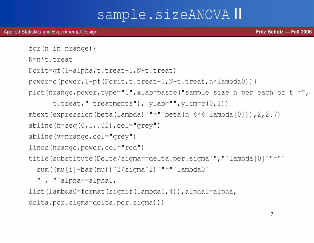
for(n in nrange){

N=n*t.treat

Fcrit=qf(1-alpha,t.treat-1,N-t.treat)

power=c(power,1-pf(Fcrit,t.treat-1,N-t.treat,n*lambda0))}

plot(nrange,power,type="l",xlab=paste("sample size n per each of t =",

t.treat," treatments"), ylab="",ylim=c(0,1))

mtext(expression(beta(lambda)˜"="˜beta(n %*% lambda[0])),2,2.7)

abline(h=seq(0,1,.02),col="grey")

abline(v=nrange,col="grey")

lines(nrange,power,col="red")

title(substitute(Delta/sigma==delta.per.sigma˜","˜lambda[0]˜"="˜

sum((mu[i]-bar(mu))ˆ2/sigmaˆ2)˜"="˜lambda0˜

" , "˜alpha==alpha1,

list(lambda0=format(signif(lambda0,4)),alpha1=alpha,

delta.per.sigma=delta.per.sigma)))

7

sample.sizeANOVA IIIApplied Statistics and Experimental Design Fritz Scholz — Fall 2006

if(!is.null(power0)){

abline(h=power0,col="blue")

par(las=2)

mtext(power0,4,0.2,at=power0,col="blue")

par(las=0)}}

8

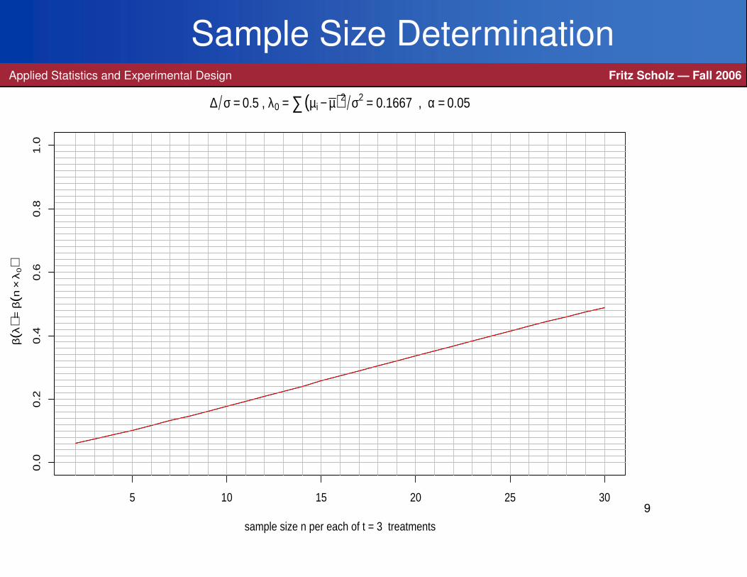
Sample Size DeterminationApplied Statistics and Experimental Design Fritz Scholz — Fall 2006

5 10 15 20 25 30

0.0

0.2

0.4

0.6

0.8

1.0

sample size n per each of t = 3 treatments

β(λ

) = β

(n×

λ0)

∆ σ = 0.5 , λ0 = ∑(µi − µ)2 σ2 = 0.1667 , α = 0.05

9

Sample Size Determination (increased n)Applied Statistics and Experimental Design Fritz Scholz — Fall 2006

30 40 50 60 70 80 90 100

0.0

0.2

0.4

0.6

0.8

1.0

sample size n per each of t = 3 treatments

β(λ

) = β

(n×

λ0)

∆ σ = 0.5 , λ0 = ∑(µi − µ)2 σ2 = 0.1667 , α = 0.05

10

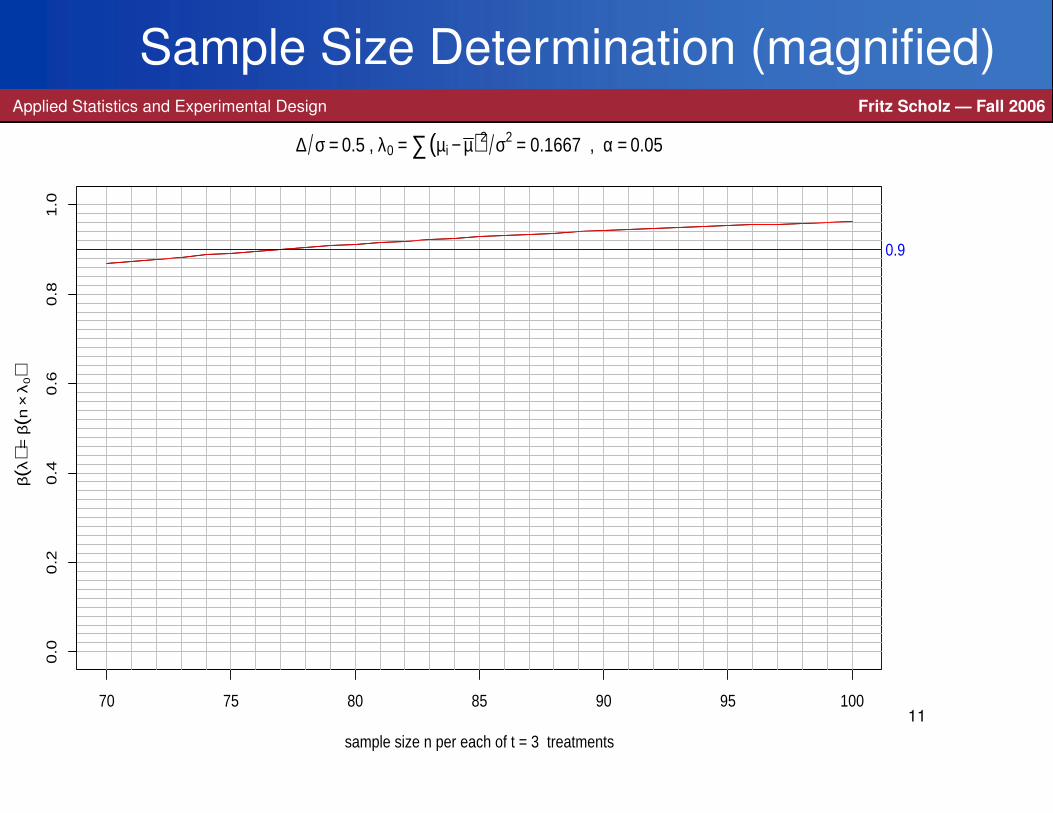
Sample Size Determination (magnified)Applied Statistics and Experimental Design Fritz Scholz — Fall 2006

70 75 80 85 90 95 100

0.0

0.2

0.4

0.6

0.8

1.0

sample size n per each of t = 3 treatments

β(λ

) = β

(n×

λ0)

∆ σ = 0.5 , λ0 = ∑(µi − µ)2 σ2 = 0.1667 , α = 0.05

0.9

11

Coagulation ExampleApplied Statistics and Experimental Design Fritz Scholz — Fall 2006

In order to understand the blood coagulation behavior in relation to various diets,

lab animals were given 4 different diets and their subsequent blood draws were

then measured for their respective coagulation times in seconds.

The lab animals were assigned randomly to the various diets.

The results were as follows:

> ctime

[1] 59 60 62 63 63 64 65 66 67 71 66 67 68 68 68 71 56 59

[19] 60 61 62 63 63 64

> diet

[1] "A" "A" "A" "A" "B" "B" "B" "B" "B" "B" "C" "C" "C"

[14] "C" "C" "C" "D" "D" "D" "D" "D" "D" "D" "D"

12

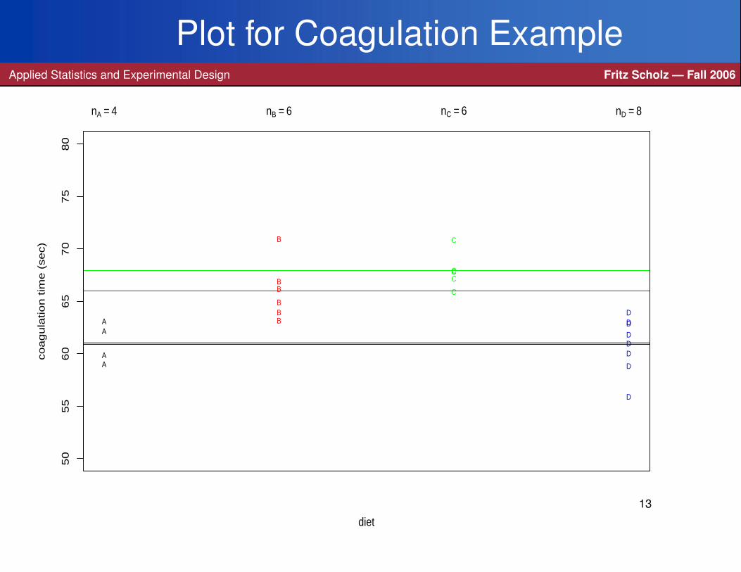
Plot for Coagulation ExampleApplied Statistics and Experimental Design Fritz Scholz — Fall 2006

AA

AA B

BB

BB

B

C

CCCC

C

D

D

DDD

DDD

diet

co

ag

ula

tio

n t

ime

(se

c)

50

55

60

65

70

75

80

nA = 4 nB = 6 nC = 6 nD = 8

13

ANOVA for Coagulation ExampleApplied Statistics and Experimental Design Fritz Scholz — Fall 2006

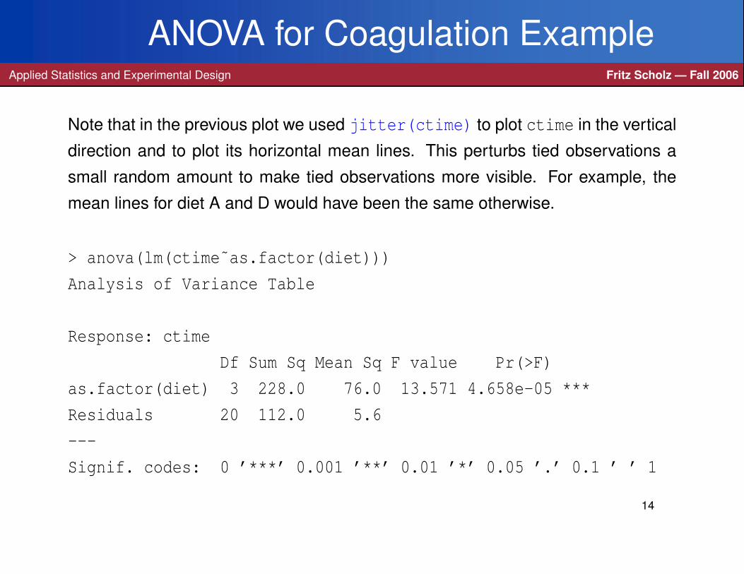
Note that in the previous plot we used jitter(ctime) to plot ctime in the vertical

direction and to plot its horizontal mean lines. This perturbs tied observations a

small random amount to make tied observations more visible. For example, the

mean lines for diet A and D would have been the same otherwise.

> anova(lm(ctime˜as.factor(diet)))

Analysis of Variance Table

Response: ctime

Df Sum Sq Mean Sq F value Pr(>F)

as.factor(diet) 3 228.0 76.0 13.571 4.658e-05 ***

Residuals 20 112.0 5.6

---

Signif. codes: 0 ’***’ 0.001 ’**’ 0.01 ’*’ 0.05 ’.’ 0.1 ’ ’ 1

14

lm for Coagulation ExampleApplied Statistics and Experimental Design Fritz Scholz — Fall 2006

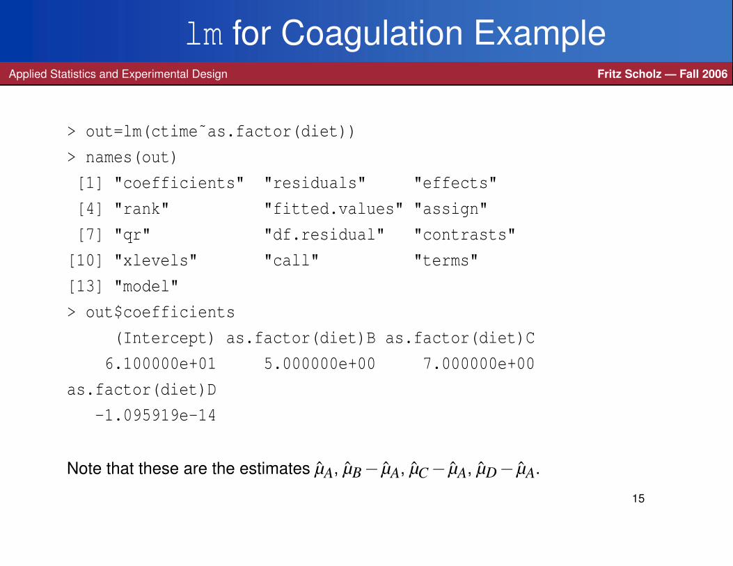
> out=lm(ctime˜as.factor(diet))

> names(out)

[1] "coefficients" "residuals" "effects"

[4] "rank" "fitted.values" "assign"

[7] "qr" "df.residual" "contrasts"

[10] "xlevels" "call" "terms"

[13] "model"

> out$coefficients

(Intercept) as.factor(diet)B as.factor(diet)C

6.100000e+01 5.000000e+00 7.000000e+00

as.factor(diet)D

-1.095919e-14

Note that these are the estimates µA, µB− µA, µC− µA, µD− µA.

15

Residuals from lm for Coagulation ExampleApplied Statistics and Experimental Design Fritz Scholz — Fall 2006

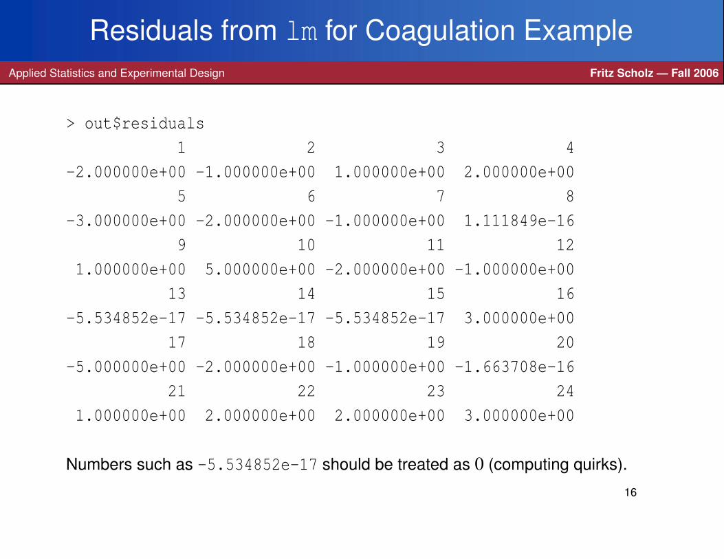
> out$residuals

1 2 3 4

-2.000000e+00 -1.000000e+00 1.000000e+00 2.000000e+00

5 6 7 8

-3.000000e+00 -2.000000e+00 -1.000000e+00 1.111849e-16

9 10 11 12

1.000000e+00 5.000000e+00 -2.000000e+00 -1.000000e+00

13 14 15 16

-5.534852e-17 -5.534852e-17 -5.534852e-17 3.000000e+00

17 18 19 20

-5.000000e+00 -2.000000e+00 -1.000000e+00 -1.663708e-16

21 22 23 24

1.000000e+00 2.000000e+00 2.000000e+00 3.000000e+00

Numbers such as -5.534852e-17 should be treated as 0 (computing quirks).

16

Fitted Values from lm for Coagulation ExampleApplied Statistics and Experimental Design Fritz Scholz — Fall 2006

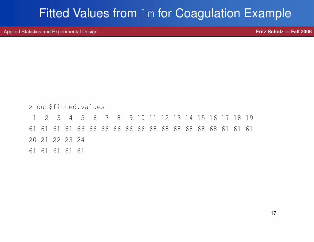
> out$fitted.values

1 2 3 4 5 6 7 8 9 10 11 12 13 14 15 16 17 18 19

61 61 61 61 66 66 66 66 66 66 68 68 68 68 68 68 61 61 61

20 21 22 23 24

61 61 61 61 61

17

Comparing Treatment Means Yi.Applied Statistics and Experimental Design Fritz Scholz — Fall 2006

When the hypothesis H0 : µ1 = . . . = µt is not rejected at level α then there is

little purpose in looking closer at differences between the sample means Yi.for the various treatments.

Any such perceived differences could easily have come about by

simple random variation, even when the hypothesis is true.

Why then read something into randomness? It is like reading tea leaves!

However, when the hypothesis is rejected it is quite natural to ask

in which way the hypothesis was contradicted.

The best indicators for any analysis as to how the means µi may be different

would be the sample or treatment means µi = Yi., i = 1, . . . , t.18

Confidence Intervals for µiApplied Statistics and Experimental Design Fritz Scholz — Fall 2006

A first step in understanding differences in the µi is to look at their estimates µi = Yi..

We should do this in the context of the sampling variability of µi.

In the past we addressed this via confidence intervals for µi based on µi.

In any such confidence interval we can now use the pooled variance s2

from all t samples and not just the variance s2i from the ith sample, i.e. we get

µi± t1−α/2,N−t×s√

nias our 100(1−α)% confidence interval for µi.

This follows as before (exercise) from the independence of µi and s, the fact that

(µi−µi)/(σ/√

ni)∼N (0,1), and from s2/σ2 ∼ χ2N−t/(N− t).

The validity of this improvement (N− t � ni−1 when using s2 instead of s2i )

depends strongly on the assumption that the population variances σ2 behind all

t samples are the same, or at least approximately so.

19

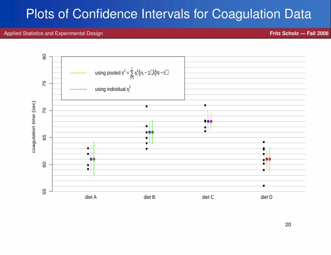
Plots of Confidence Intervals for Coagulation DataApplied Statistics and Experimental Design Fritz Scholz — Fall 2006

co

ag

ula

tio

n t

ime

(se

c)

diet A diet B diet C diet D

55

60

65

70

75

80

●

●

●

●●

●

●

●

using pooled s2 = ∑i=1

t

si2(ni − 1) (N − t)

using individual si2

●

●

●

● ●

●

●

●

●

●

●

●

●●●

●

●

●

●

●

●

●●

●

20

Simultaneous Confidence IntervalsApplied Statistics and Experimental Design Fritz Scholz — Fall 2006

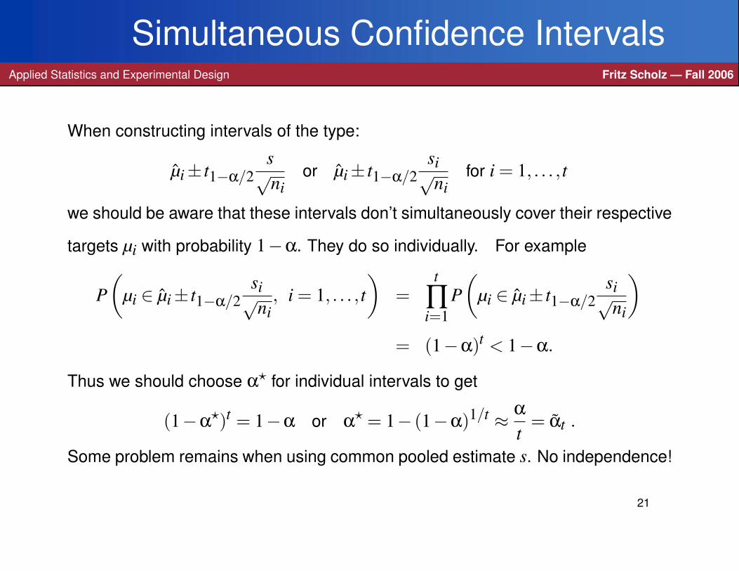
When constructing intervals of the type:

µi± t1−α/2s√

nior µi± t1−α/2

si√ni

for i = 1, . . . , t

we should be aware that these intervals don’t simultaneously cover their respective

targets µi with probability 1−α. They do so individually. For example

P(

µi ∈ µi± t1−α/2si√ni

, i = 1, . . . , t)

=t

∏i=1

P(

µi ∈ µi± t1−α/2si√ni

)= (1−α)t < 1−α.

Thus we should choose α? for individual intervals to get

(1−α?)t = 1−α or α

? = 1− (1−α)1/t ≈ α

t= αt .

Some problem remains when using common pooled estimate s. No independence!

21

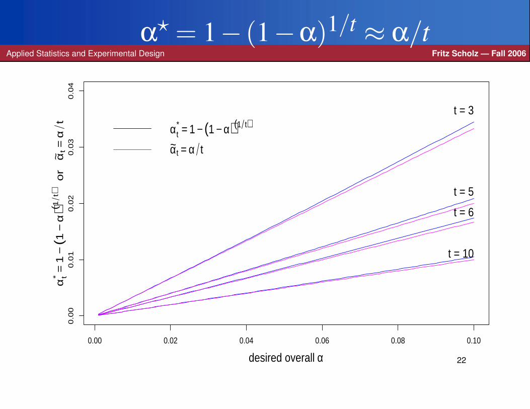
α? = 1− (1−α)1/t ≈ α/tApplied Statistics and Experimental Design Fritz Scholz — Fall 2006

0.00 0.02 0.04 0.06 0.08 0.10

0.0

00

.01

0.0

20

.03

0.0

4

desired overall α

αt*

=1

−(1

−α

)(1t)

or

α~

t=

αt

t = 10

t = 3

t = 5

t = 6

αt* = 1 − (1 − α)(1 t)

α~t = α t

22

Dealing with Dependence from Using Pooled sApplied Statistics and Experimental Design Fritz Scholz — Fall 2006

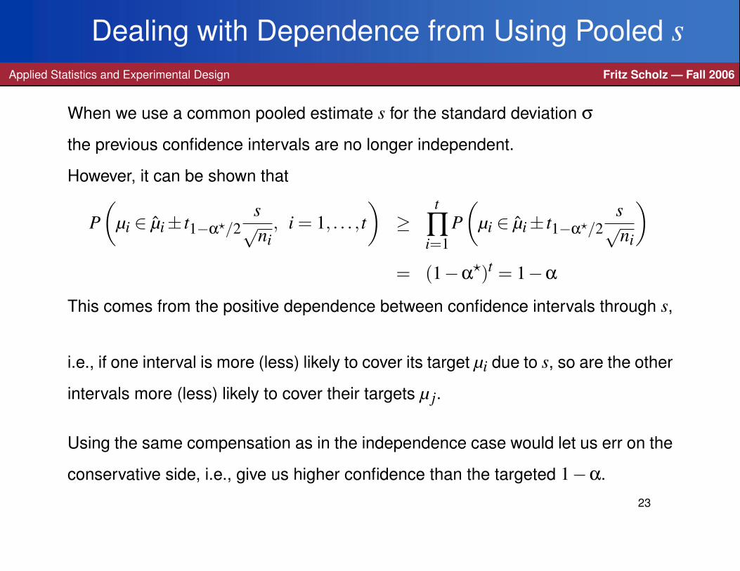
When we use a common pooled estimate s for the standard deviation σ

the previous confidence intervals are no longer independent.

However, it can be shown that

P(

µi ∈ µi± t1−α?/2s√

ni, i = 1, . . . , t

)≥

t

∏i=1

P(

µi ∈ µi± t1−α?/2s√

ni

)= (1−α

?)t = 1−α

This comes from the positive dependence between confidence intervals through s,

i.e., if one interval is more (less) likely to cover its target µi due to s, so are the other

intervals more (less) likely to cover their targets µ j.

Using the same compensation as in the independence case would let us err on the

conservative side, i.e., give us higher confidence than the targeted 1−α.

23

Boole’s and Bonferroni’s InequalityApplied Statistics and Experimental Design Fritz Scholz — Fall 2006

For any m events E1, . . . ,Em Boole’s inequality states

P(E1∪ . . .∪Em)≤ P(E1)+ . . .+P(Em)

For any m events E1, . . . ,Em Bonferroni’s inequality states

P(E1∩ . . .∩Em)≥ 1−m

∑i=1

(1−P(Ei))

The statement are equivalent, since P(E1∪ . . .∪Em) = 1−P(Ec1∩ . . .∩Ec

m).

If Ei denotes the ith coverage event{

µi ∈ µi± t1−α/2s√ni

}with P(Ei) = 1− α,

then the simultaneous coverage probability is bounded from below as follows

P

(t\

i=1Ei

)≥ 1−

t

∑i=1

(1−P(Ei)) = 1− tα = 1−α if α = αt = α/t ,

i.e., we can achieve at least 1−α probability coverage by choosing the individualcoverage appropriately, namely 1− α = 1−α/t. Almost same adjustment.

24

ContrastsApplied Statistics and Experimental Design Fritz Scholz — Fall 2006

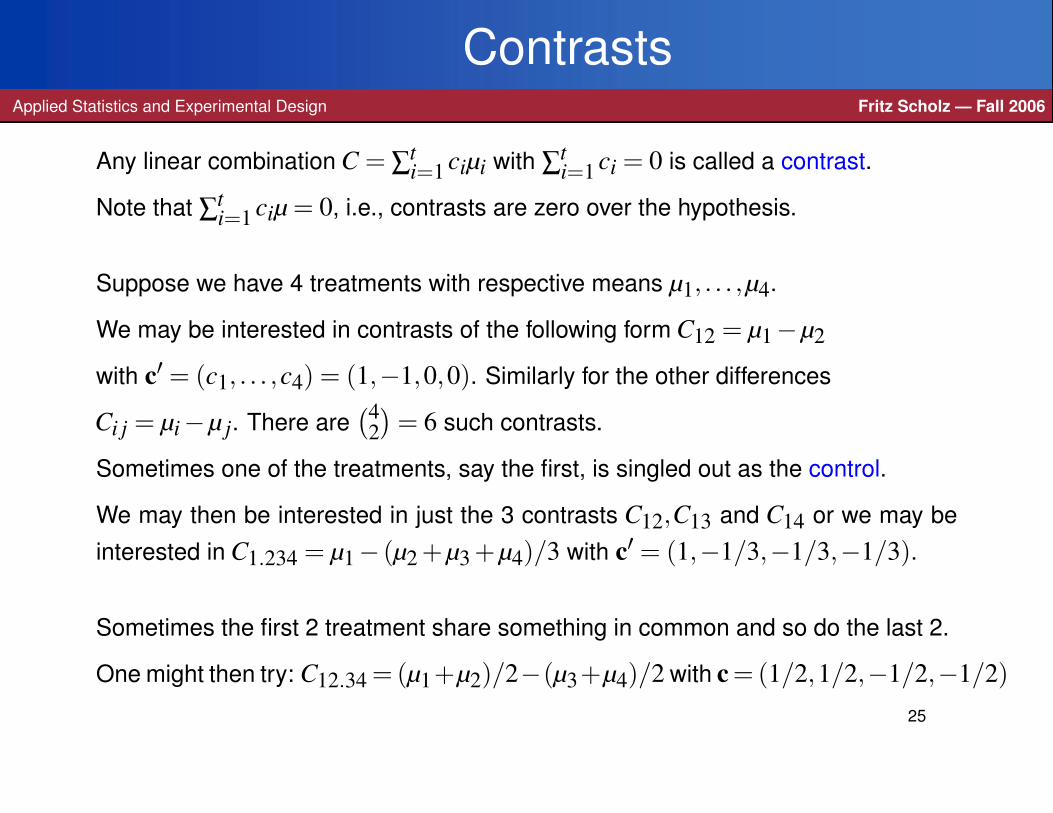
Any linear combination C = ∑ti=1 ciµi with ∑

ti=1 ci = 0 is called a contrast.

Note that ∑ti=1 ciµ = 0, i.e., contrasts are zero over the hypothesis.

Suppose we have 4 treatments with respective means µ1, . . . ,µ4.

We may be interested in contrasts of the following form C12 = µ1−µ2

with c′ = (c1, . . . ,c4) = (1,−1,0,0). Similarly for the other differences

Ci j = µi−µ j. There are(4

2)

= 6 such contrasts.

Sometimes one of the treatments, say the first, is singled out as the control.

We may then be interested in just the 3 contrasts C12,C13 and C14 or we may be

interested in C1.234 = µ1− (µ2 +µ3 +µ4)/3 with c′ = (1,−1/3,−1/3,−1/3).

Sometimes the first 2 treatment share something in common and so do the last 2.

One might then try: C12.34 =(µ1+µ2)/2−(µ3+µ4)/2 with c =(1/2,1/2,−1/2,−1/2)25

Estimates and Confidence Intervals for ContrastsApplied Statistics and Experimental Design Fritz Scholz — Fall 2006

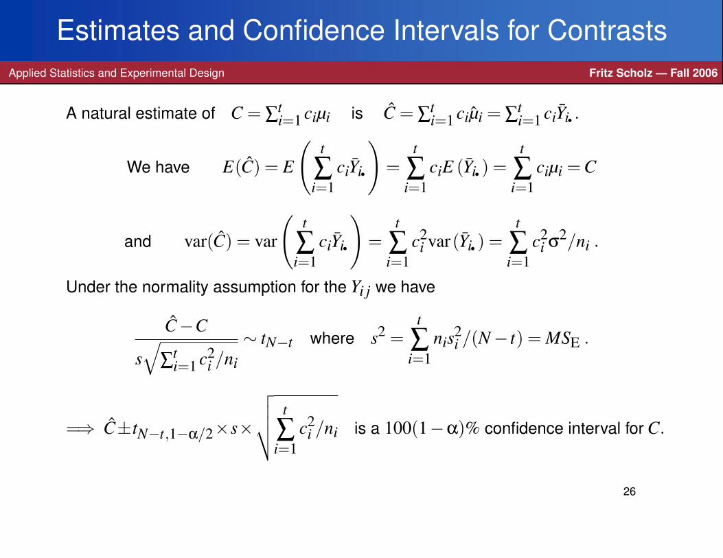
A natural estimate of C = ∑ti=1 ciµi is C = ∑

ti=1 ciµi = ∑

ti=1 ciYi..

We have E(C) = E

(t

∑i=1

ciYi.)

=t

∑i=1

ciE (Yi.) =t

∑i=1

ciµi = C

and var(C) = var

(t

∑i=1

ciYi.)

=t

∑i=1

c2i var(Yi.) =

t

∑i=1

c2i σ

2/ni .

Under the normality assumption for the Yi j we have

C−C

s√

∑ti=1 c2

i /ni

∼ tN−t where s2 =t

∑i=1

nis2i /(N− t) = MSE .

=⇒ C±tN−t,1−α/2×s×

√√√√ t

∑i=1

c2i /ni is a 100(1−α)% confidence interval for C.

26

Testing H0 : C = 0Applied Statistics and Experimental Design Fritz Scholz — Fall 2006

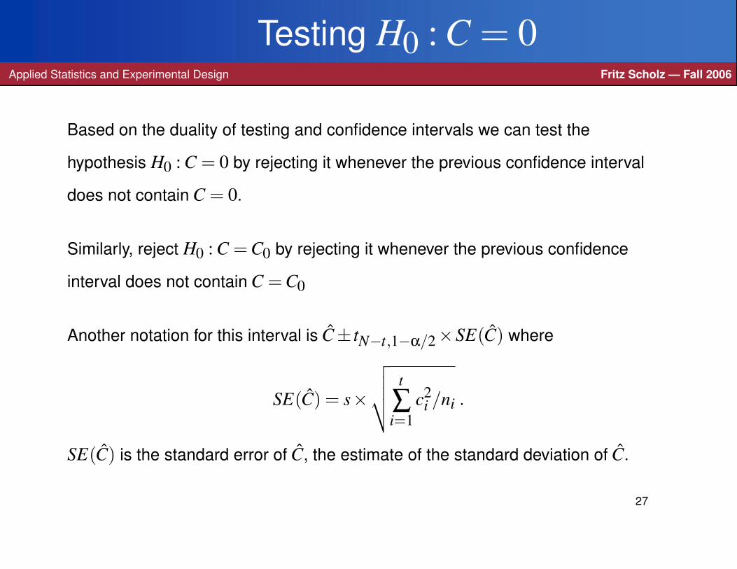
Based on the duality of testing and confidence intervals we can test the

hypothesis H0 : C = 0 by rejecting it whenever the previous confidence interval

does not contain C = 0.

Similarly, reject H0 : C = C0 by rejecting it whenever the previous confidence

interval does not contain C = C0

Another notation for this interval is C± tN−t,1−α/2×SE(C) where

SE(C) = s×

√√√√ t

∑i=1

c2i /ni .

SE(C) is the standard error of C, the estimate of the standard deviation of C.

27

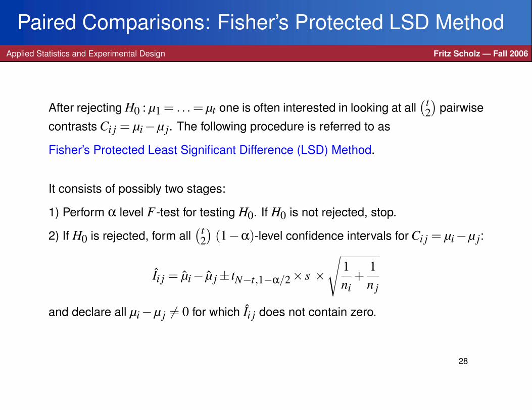
Paired Comparisons: Fisher’s Protected LSD MethodApplied Statistics and Experimental Design Fritz Scholz — Fall 2006

After rejecting H0 : µ1 = . . . = µt one is often interested in looking at all(t

2)

pairwise

contrasts Ci j = µi−µ j. The following procedure is referred to as

Fisher’s Protected Least Significant Difference (LSD) Method.

It consists of possibly two stages:

1) Perform α level F-test for testing H0. If H0 is not rejected, stop.

2) If H0 is rejected, form all(t

2)

(1−α)-level confidence intervals for Ci j = µi−µ j:

Ii j = µi− µ j± tN−t,1−α/2× s ×√

1ni

+1n j

and declare all µi−µ j 6= 0 for which Ii j does not contain zero.

28

Comments on Fisher’s Protected LSD MethodApplied Statistics and Experimental Design Fritz Scholz — Fall 2006

If H0 is true, the chance of making any statements contradicting H0 is at most α.

This is the protected aspect of this procedure.

However, when H0 is not true there are many possible contingencies, some of

which can give us a higher than desired chance of pronouncing a significant

difference, when in fact there is none.

E.g., if all but one mean (say µ1) are equal and µ1 is far away from µ2 = . . . = µt

our chance of rejecting H0 is almost 1.

However, among the intervals for µi−µ j, 2≤ i < j we may find a significantly

higher than α proportion of cases with wrongly declared differences.

This is due to the multiple comparison issue.

29

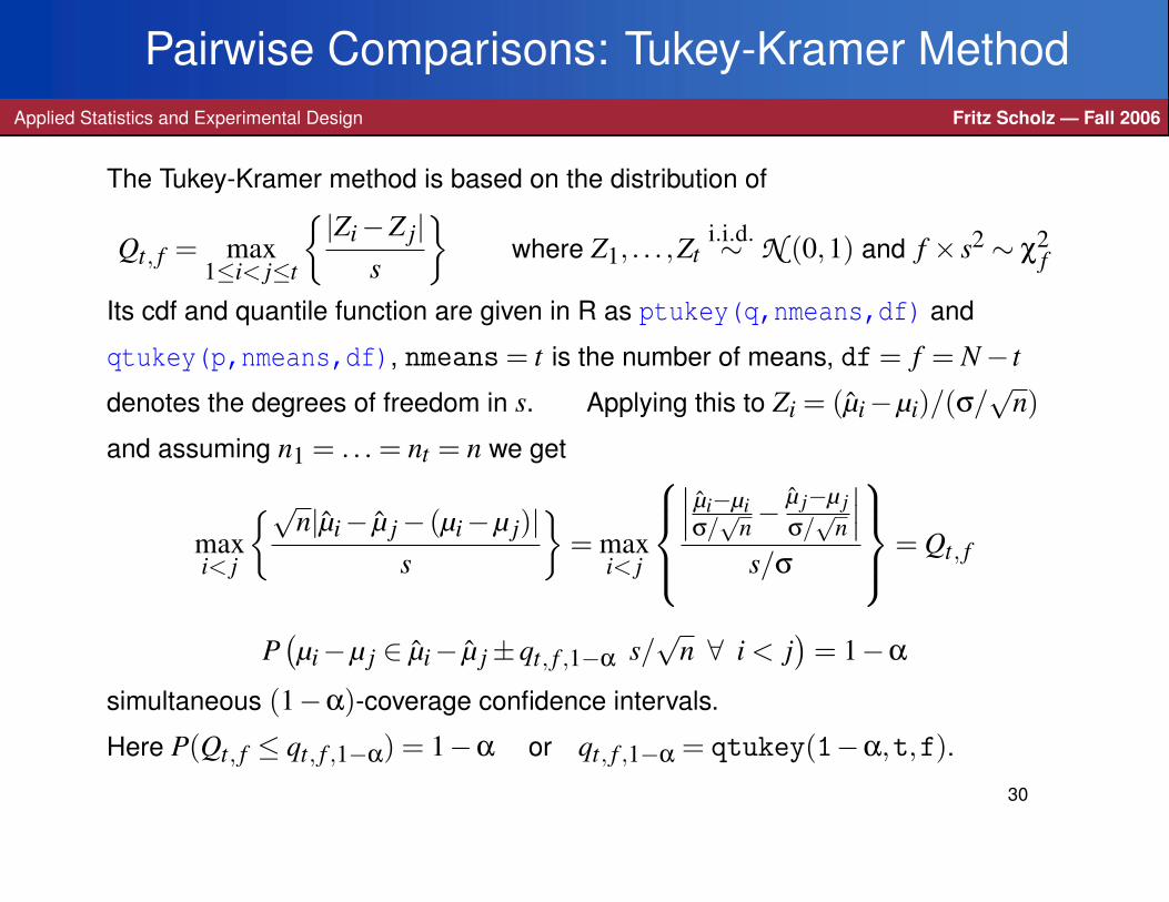
Pairwise Comparisons: Tukey-Kramer MethodApplied Statistics and Experimental Design Fritz Scholz — Fall 2006

The Tukey-Kramer method is based on the distribution of

Qt, f = max1≤i< j≤t

{|Zi−Z j|s

}where Z1, . . . ,Zt

i.i.d.∼ N (0,1) and f × s2 ∼ χ2f

Its cdf and quantile function are given in R as ptukey(q,nmeans,df) and

qtukey(p,nmeans,df), nmeans = t is the number of means, df = f = N− t

denotes the degrees of freedom in s. Applying this to Zi = (µi−µi)/(σ/√

n)

and assuming n1 = . . . = nt = n we get

maxi< j

{√n|µi− µ j− (µi−µ j)|

s

}= max

i< j

∣∣∣ µi−µiσ/√

n−µ j−µ jσ/√

n

∣∣∣s/σ

= Qt, f

P(µi−µ j ∈ µi− µ j±qt, f ,1−α s/

√n ∀ i < j

)= 1−α

simultaneous (1−α)-coverage confidence intervals.

Here P(Qt, f ≤ qt, f ,1−α) = 1−α or qt, f ,1−α = qtukey(1−α,t,f).

30

Tukey-Kramer Method: Unequal Sample SizesApplied Statistics and Experimental Design Fritz Scholz — Fall 2006

The simultaneous intervals for all pairwise mean differences was due to Tukey,

but it was hampered by the requirement of equal sample sizes.

This was addressed by Kramer in the following way. In the above confidence

intervals replace n in 1/√

n =√

1/n by n?i j, where n?

i j is the harmonic mean

of ni and n j, i.e., 1/n?i j = (1/ni +1/n j)/2. Different adjustment for each pair (i, j)!

It was possible to show

P(

µi−µ j ∈ µi− µ j±Qt, f ,1−α s/√

n?i j ∀ i < j

)≥ 1−α

simultaneous confidence intervals with coverage ≥ 1−α.

31

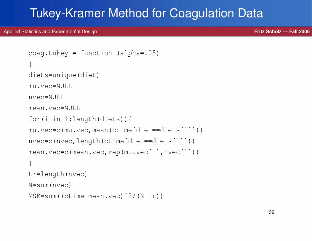
Tukey-Kramer Method for Coagulation DataApplied Statistics and Experimental Design Fritz Scholz — Fall 2006

coag.tukey = function (alpha=.05)

{

diets=unique(diet)

mu.vec=NULL

nvec=NULL

mean.vec=NULL

for(i in 1:length(diets)){

mu.vec=c(mu.vec,mean(ctime[diet==diets[i]]))

nvec=c(nvec,length(ctime[diet==diets[i]]))

mean.vec=c(mean.vec,rep(mu.vec[i],nvec[i]))

}

tr=length(nvec)

N=sum(nvec)

MSE=sum((ctime-mean.vec)ˆ2/(N-tr))

32

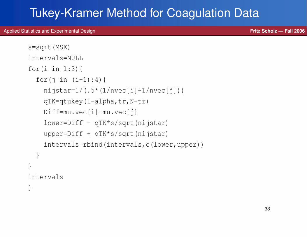
Tukey-Kramer Method for Coagulation DataApplied Statistics and Experimental Design Fritz Scholz — Fall 2006

s=sqrt(MSE)

intervals=NULL

for(i in 1:3){

for(j in (i+1):4){

nijstar=1/(.5*(1/nvec[i]+1/nvec[j]))

qTK=qtukey(1-alpha,tr,N-tr)

Diff=mu.vec[i]-mu.vec[j]

lower=Diff - qTK*s/sqrt(nijstar)

upper=Diff + qTK*s/sqrt(nijstar)

intervals=rbind(intervals,c(lower,upper))

}

}

intervals

}

33

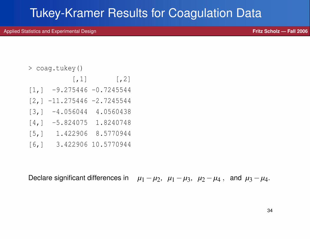
Tukey-Kramer Results for Coagulation DataApplied Statistics and Experimental Design Fritz Scholz — Fall 2006

> coag.tukey()

[,1] [,2]

[1,] -9.275446 -0.7245544

[2,] -11.275446 -2.7245544

[3,] -4.056044 4.0560438

[4,] -5.824075 1.8240748

[5,] 1.422906 8.5770944

[6,] 3.422906 10.5770944

Declare significant differences in µ1−µ2, µ1−µ3, µ2−µ4 , and µ3−µ4.

34

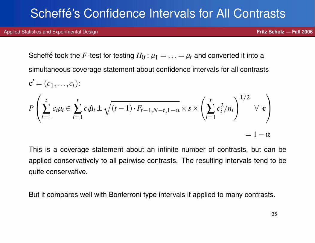
Scheffe’s Confidence Intervals for All ContrastsApplied Statistics and Experimental Design Fritz Scholz — Fall 2006

Scheffe took the F-test for testing H0 : µ1 = . . . = µt and converted it into a

simultaneous coverage statement about confidence intervals for all contrasts

c′ = (c1, . . . ,ct):

P

t

∑i=1

ciµi ∈t

∑i=1

ciµi±√

(t−1) ·Ft−1,N−t,1−α× s×

(t

∑i=1

c2i /ni

)1/2

∀ c

= 1−α

This is a coverage statement about an infinite number of contrasts, but can be

applied conservatively to all pairwise contrasts. The resulting intervals tend to be

quite conservative.

But it compares well with Bonferroni type intervals if applied to many contrasts.

35

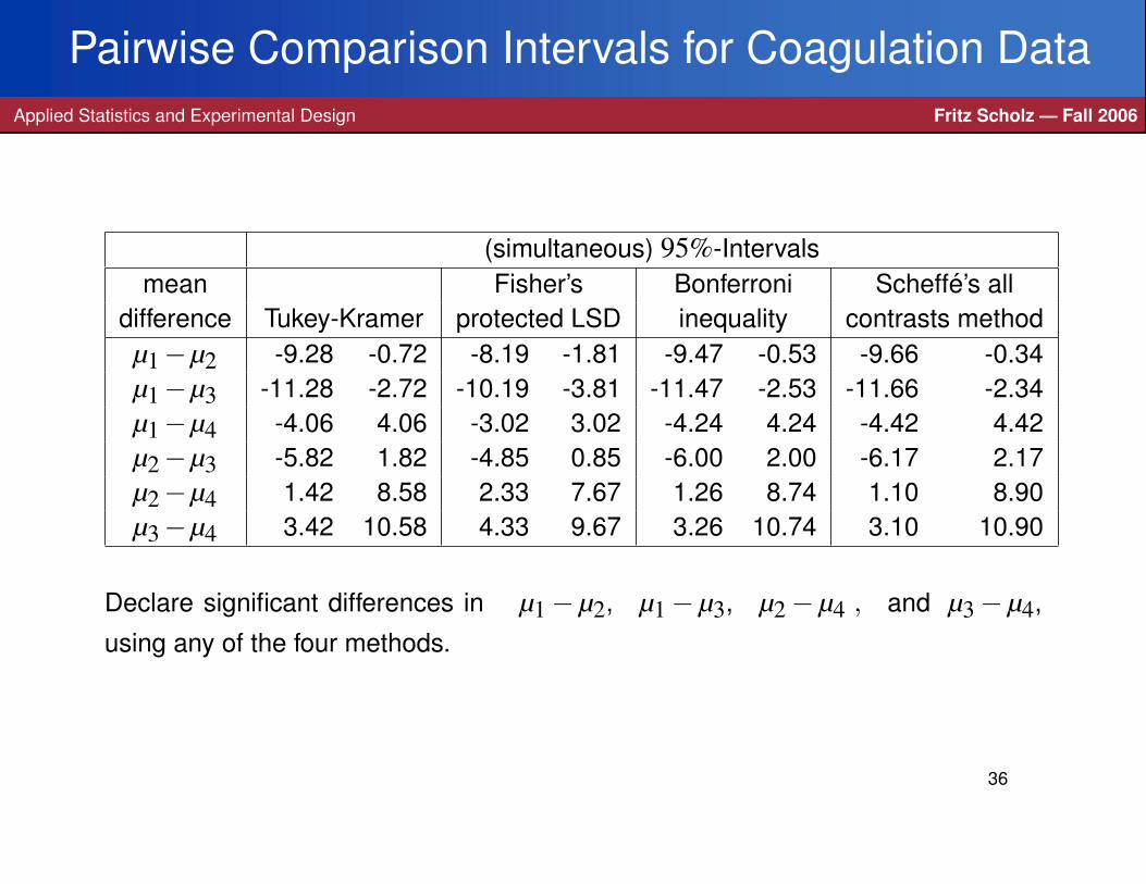
Pairwise Comparison Intervals for Coagulation DataApplied Statistics and Experimental Design Fritz Scholz — Fall 2006

(simultaneous) 95%-Intervalsmean Fisher’s Bonferroni Scheffe’s all

difference Tukey-Kramer protected LSD inequality contrasts methodµ1−µ2 -9.28 -0.72 -8.19 -1.81 -9.47 -0.53 -9.66 -0.34µ1−µ3 -11.28 -2.72 -10.19 -3.81 -11.47 -2.53 -11.66 -2.34µ1−µ4 -4.06 4.06 -3.02 3.02 -4.24 4.24 -4.42 4.42µ2−µ3 -5.82 1.82 -4.85 0.85 -6.00 2.00 -6.17 2.17µ2−µ4 1.42 8.58 2.33 7.67 1.26 8.74 1.10 8.90µ3−µ4 3.42 10.58 4.33 9.67 3.26 10.74 3.10 10.90

Declare significant differences in µ1− µ2, µ1− µ3, µ2− µ4 , and µ3− µ4,

using any of the four methods.

36

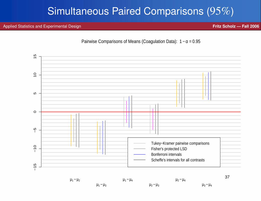
Simultaneous Paired Comparisons (95%)Applied Statistics and Experimental Design Fritz Scholz — Fall 2006

−1

5−

10

−5

05

10

15

µ1 − µ2

µ1 − µ3

µ1 − µ4

µ2 − µ3

µ2 − µ4

µ3 − µ4

Pairwise Comparisons of Means (Coagulation Data): 1 − α = 0.95

Tukey−Kramer pairwise comparisonsFisher's protected LSDBonferroni intervalsScheffe's intervals for all contrasts

37

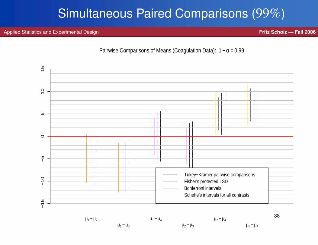
Simultaneous Paired Comparisons (99%)Applied Statistics and Experimental Design Fritz Scholz — Fall 2006

−1

5−

10

−5

05

10

15

µ1 − µ2

µ1 − µ3

µ1 − µ4

µ2 − µ3

µ2 − µ4

µ3 − µ4

Pairwise Comparisons of Means (Coagulation Data): 1 − α = 0.99

Tukey−Kramer pairwise comparisonsFisher's protected LSDBonferroni intervalsScheffe's intervals for all contrasts

38

Orthogonal ContrastApplied Statistics and Experimental Design Fritz Scholz — Fall 2006

All(t

2)

pairwise comparisons for µi−µ j could by very many and simultaneous

intervals would become quite conservative.

Since all these contrasts span a (t−1)-dimensional space one should be

able to capture all differences with just t−1 orthogonal contrasts.

C1 =t

∑i=1

c1iµi ⊥ C2 =t

∑i=1

c2iµi ⇐⇒t

∑i=1

c1ic2i/ni = 0(

wrong def. inMontgomery p.91

)C1 ⊥C2 =⇒ cov(C1,C2) =

t

∑i=1

t

∑j=1

c1ic2 jcov(µi, µ j) =t

∑i=1

c1ic2iσ2/ni = 0 ,

i.e., C1 and C2 are independent and simultaneous statements for C1,C2, . . . are

easier to handle, just as before when making simultaneous intervals for µ1, . . . ,µt

based on independent µ1, . . . , µt .

The trick is to have meaningful or interpretable orthogonal contrast.

39

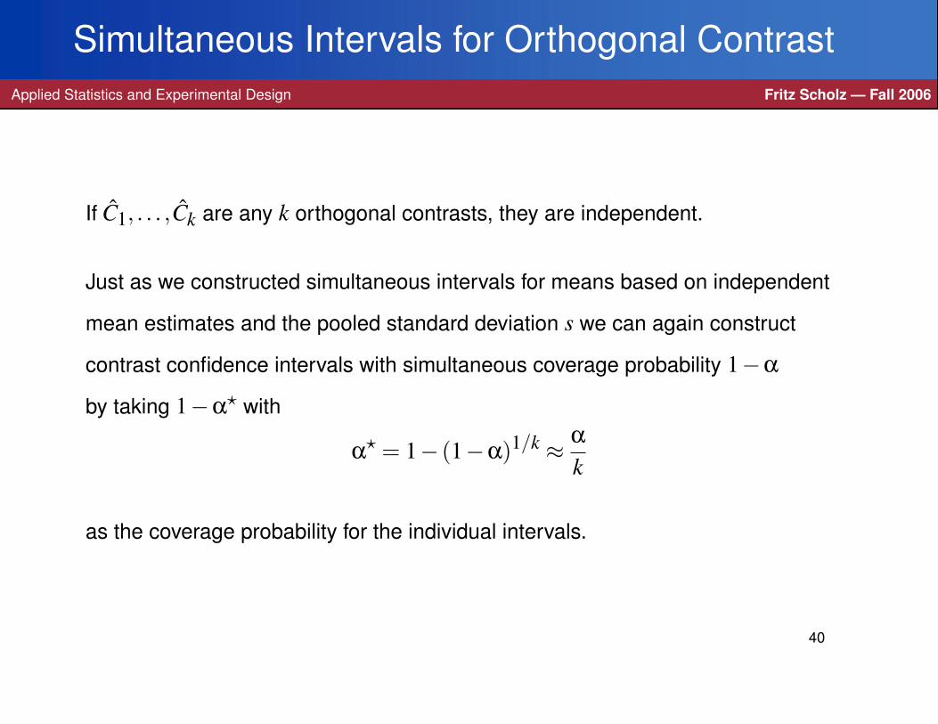
Simultaneous Intervals for Orthogonal ContrastApplied Statistics and Experimental Design Fritz Scholz — Fall 2006

If C1, . . . ,Ck are any k orthogonal contrasts, they are independent.

Just as we constructed simultaneous intervals for means based on independent

mean estimates and the pooled standard deviation s we can again construct

contrast confidence intervals with simultaneous coverage probability 1−α

by taking 1−α? with

α? = 1− (1−α)1/k ≈ α

k

as the coverage probability for the individual intervals.

40

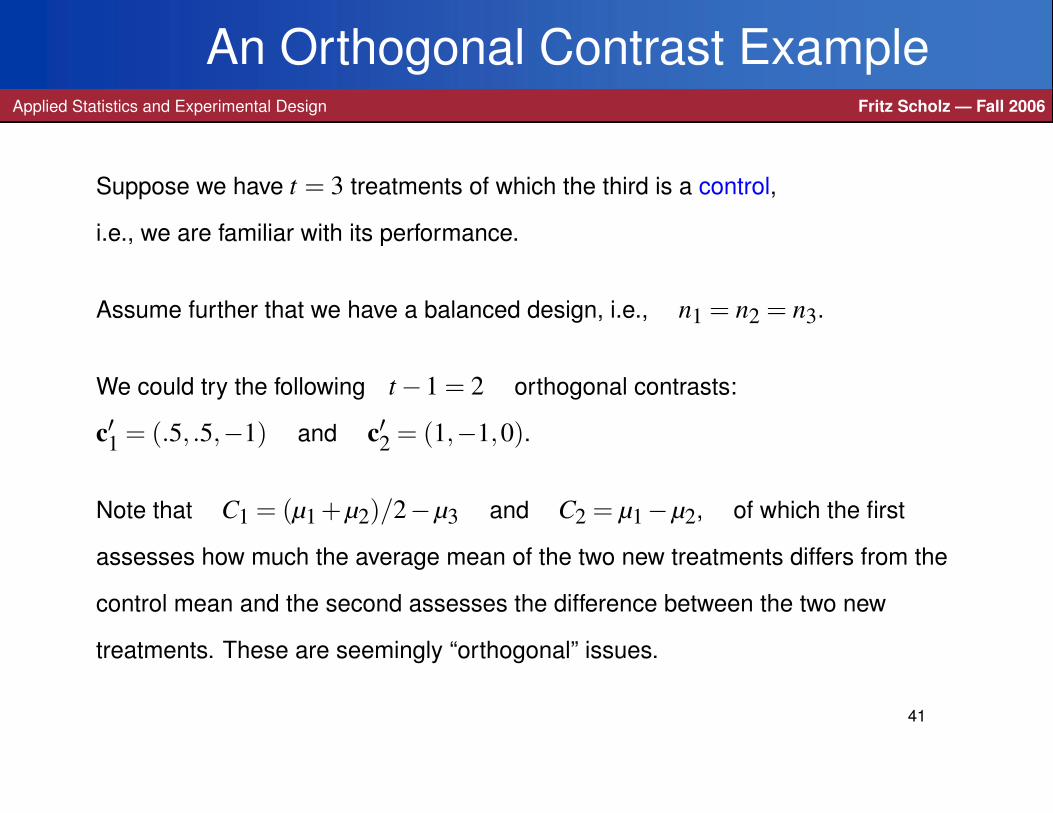
An Orthogonal Contrast ExampleApplied Statistics and Experimental Design Fritz Scholz — Fall 2006

Suppose we have t = 3 treatments of which the third is a control,

i.e., we are familiar with its performance.

Assume further that we have a balanced design, i.e., n1 = n2 = n3.

We could try the following t−1 = 2 orthogonal contrasts:

c′1 = (.5, .5,−1) and c′2 = (1,−1,0).

Note that C1 = (µ1 +µ2)/2−µ3 and C2 = µ1−µ2, of which the first

assesses how much the average mean of the two new treatments differs from the

control mean and the second assesses the difference between the two new

treatments. These are seemingly “orthogonal” issues.

41

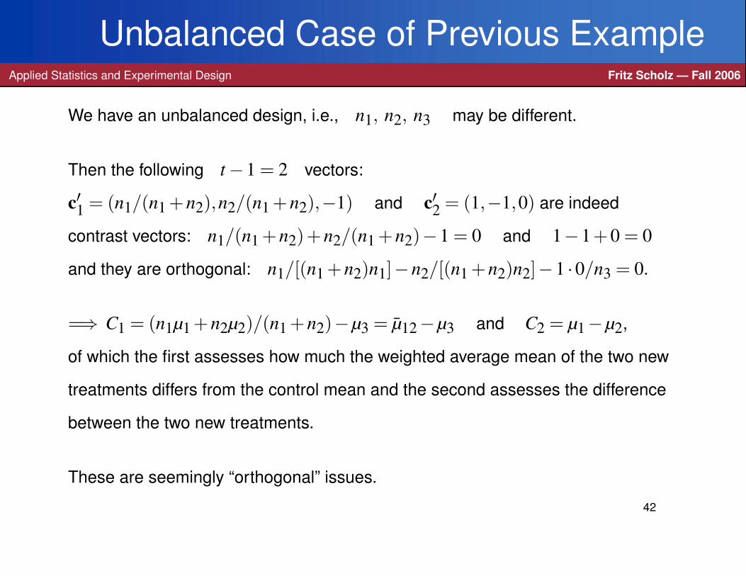
Unbalanced Case of Previous ExampleApplied Statistics and Experimental Design Fritz Scholz — Fall 2006

We have an unbalanced design, i.e., n1, n2, n3 may be different.

Then the following t−1 = 2 vectors:

c′1 = (n1/(n1 +n2),n2/(n1 +n2),−1) and c′2 = (1,−1,0) are indeed

contrast vectors: n1/(n1 +n2)+n2/(n1 +n2)−1 = 0 and 1−1+0 = 0

and they are orthogonal: n1/[(n1 +n2)n1]−n2/[(n1 +n2)n2]−1 ·0/n3 = 0.

=⇒ C1 = (n1µ1 +n2µ2)/(n1 +n2)−µ3 = µ12−µ3 and C2 = µ1−µ2,

of which the first assesses how much the weighted average mean of the two new

treatments differs from the control mean and the second assesses the difference

between the two new treatments.

These are seemingly “orthogonal” issues.

42

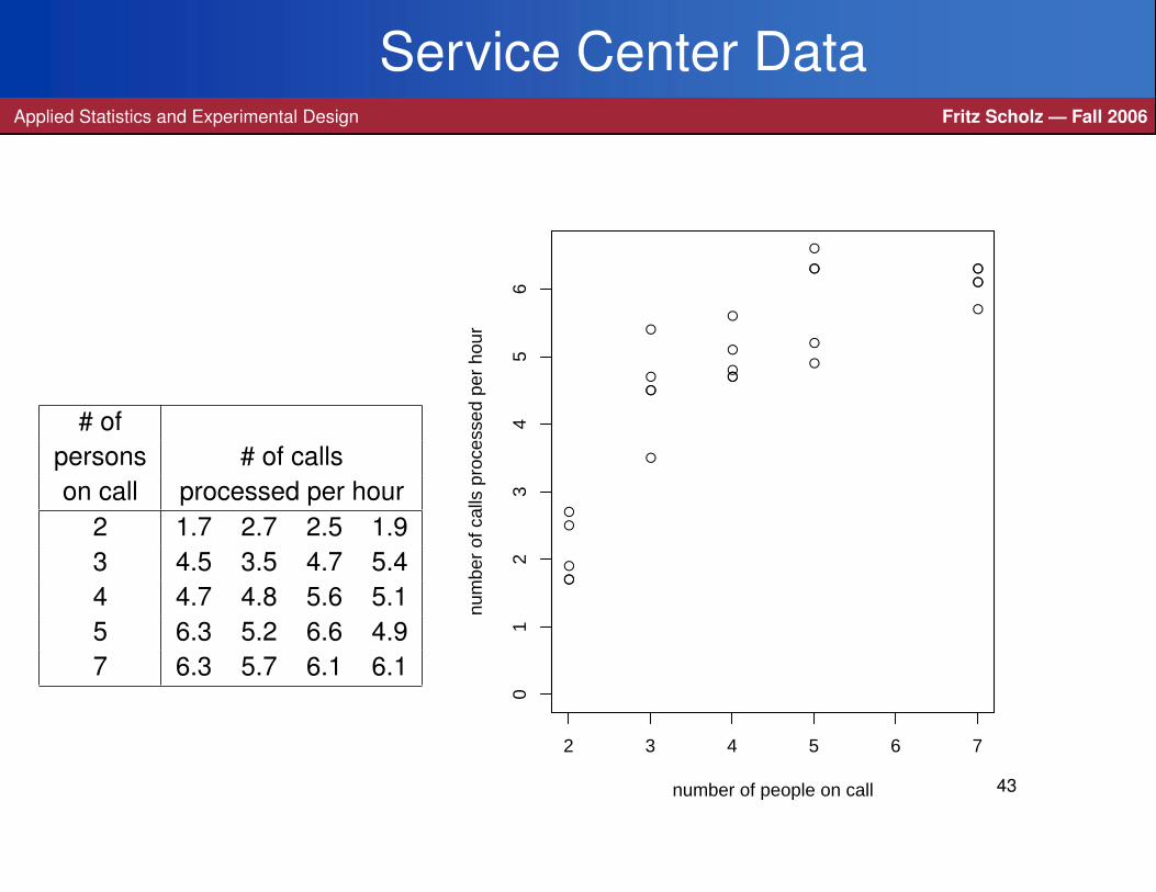
Service Center DataApplied Statistics and Experimental Design Fritz Scholz — Fall 2006

# ofpersons # of callson call processed per hour

2 1.7 2.7 2.5 1.93 4.5 3.5 4.7 5.44 4.7 4.8 5.6 5.15 6.3 5.2 6.6 4.97 6.3 5.7 6.1 6.1

●

●●

● ●

2 3 4 5 6 7

01

23

45

6

number of people on call

num

ber

of c

alls

pro

cess

ed p

er h

our

●

●●

● ●

●

●

●

●

●

●

●

●

●

●

●

●

●●

●

43

Service Center DataApplied Statistics and Experimental Design Fritz Scholz — Fall 2006

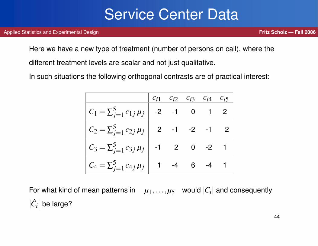
Here we have a new type of treatment (number of persons on call), where the

different treatment levels are scalar and not just qualitative.

In such situations the following orthogonal contrasts are of practical interest:

ci1 ci2 ci3 ci4 ci5

C1 = ∑5j=1 c1 j µ j -2 -1 0 1 2

C2 = ∑5j=1 c2 j µ j 2 -1 -2 -1 2

C3 = ∑5j=1 c3 j µ j -1 2 0 -2 1

C4 = ∑5j=1 c4 j µ j 1 -4 6 -4 1

For what kind of mean patterns in µ1, . . . ,µ5 would |Ci| and consequently

|Ci| be large?

44

Orthogonal Contrast PlotsApplied Statistics and Experimental Design Fritz Scholz — Fall 2006

●

●

●

●

●

−2 −1 0 1 2

−4

−2

02

46

j

Ci=

∑ j=15

ci,

j×

j u

sin

g

µj=

j

●

●

●

●

●

●

●

●

●

●●

●

●

●

●

C1

C2

C3

C4

45

Interpretation of Orthogonal Contrast PlotsApplied Statistics and Experimental Design Fritz Scholz — Fall 2006

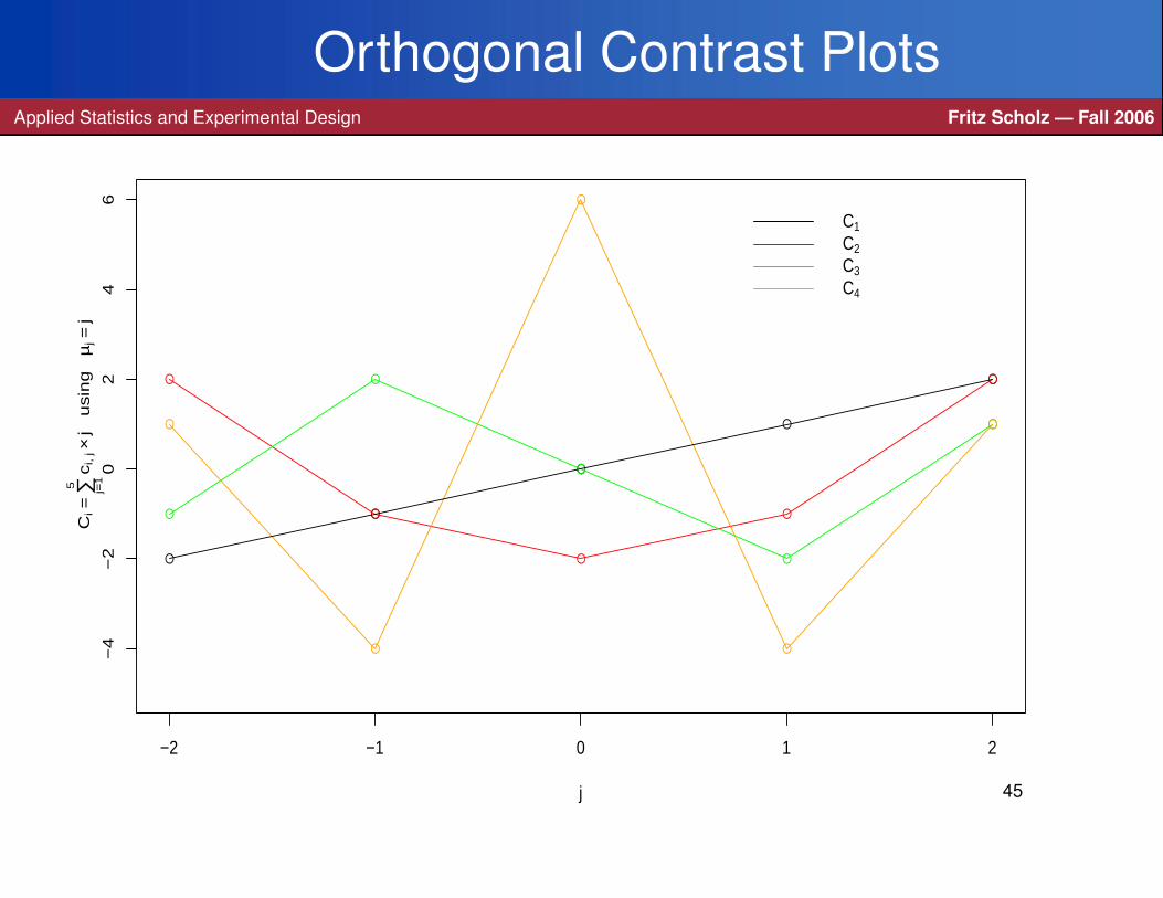
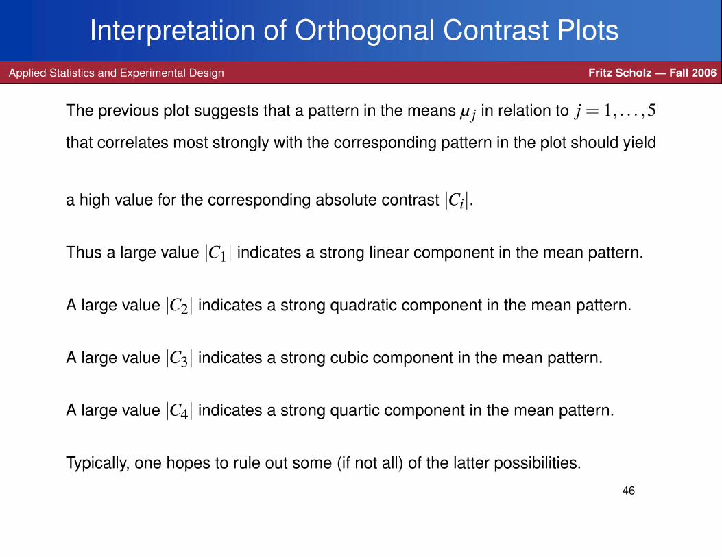
The previous plot suggests that a pattern in the means µ j in relation to j = 1, . . . ,5

that correlates most strongly with the corresponding pattern in the plot should yield

a high value for the corresponding absolute contrast |Ci|.

Thus a large value |C1| indicates a strong linear component in the mean pattern.

A large value |C2| indicates a strong quadratic component in the mean pattern.

A large value |C3| indicates a strong cubic component in the mean pattern.

A large value |C4| indicates a strong quartic component in the mean pattern.

Typically, one hopes to rule out some (if not all) of the latter possibilities.

46

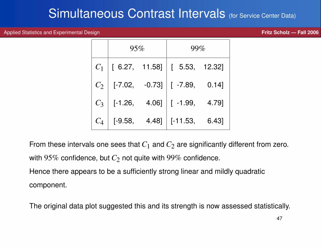
Simultaneous Contrast Intervals (for Service Center Data)

Applied Statistics and Experimental Design Fritz Scholz — Fall 2006

95% 99%

C1 [ 6.27, 11.58] [ 5.53, 12.32]

C2 [-7.02, -0.73] [ -7.89, 0.14]

C3 [-1.26, 4.06] [ -1.99, 4.79]

C4 [-9.58, 4.48] [-11.53, 6.43]

From these intervals one sees that C1 and C2 are significantly different from zero.

with 95% confidence, but C2 not quite with 99% confidence.

Hence there appears to be a sufficiently strong linear and mildly quadratic

component.

The original data plot suggested this and its strength is now assessed statistically.

47

Orthogonal Polynomial Contrast VectorsApplied Statistics and Experimental Design Fritz Scholz — Fall 2006

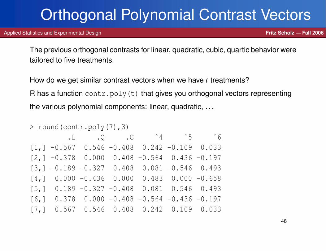
The previous orthogonal contrasts for linear, quadratic, cubic, quartic behavior weretailored to five treatments.

How do we get similar contrast vectors when we have t treatments?

R has a function contr.poly(t) that gives you orthogonal vectors representing

the various polynomial components: linear, quadratic, . . .

> round(contr.poly(7),3).L .Q .C ˆ4 ˆ5 ˆ6

[1,] -0.567 0.546 -0.408 0.242 -0.109 0.033[2,] -0.378 0.000 0.408 -0.564 0.436 -0.197[3,] -0.189 -0.327 0.408 0.081 -0.546 0.493[4,] 0.000 -0.436 0.000 0.483 0.000 -0.658[5,] 0.189 -0.327 -0.408 0.081 0.546 0.493[6,] 0.378 0.000 -0.408 -0.564 -0.436 -0.197[7,] 0.567 0.546 0.408 0.242 0.109 0.033

48

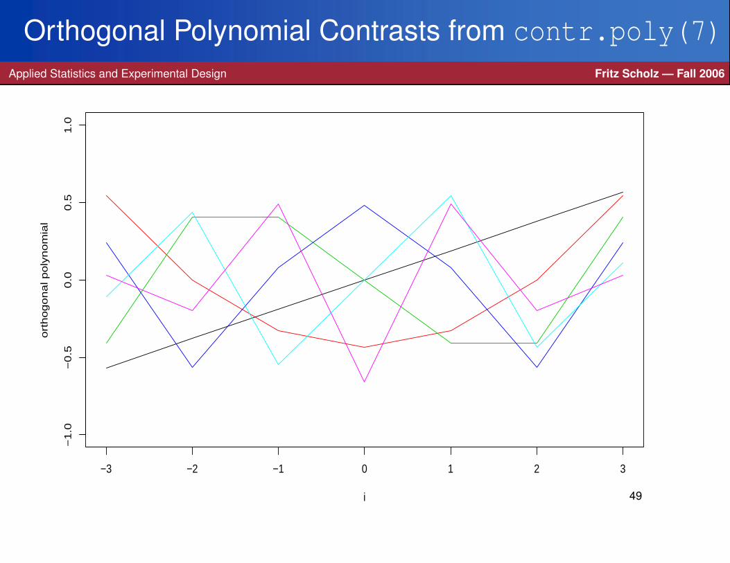
Orthogonal Polynomial Contrasts from contr.poly(7)Applied Statistics and Experimental Design Fritz Scholz — Fall 2006

−3 −2 −1 0 1 2 3

−1

.0−

0.5

0.0

0.5

1.0

i

ort

ho

go

na

l p

oly

no

mia

l

49