Frequency Response (I&N Chap 12) - UBC ECE |...
22
Slide 3.1 Frequency Response (I&N Chap 12) • Introduction & TFs • Decibel Scale & Bode Plots • Resonance • Scaling • Filter Networks • Applications/Design Frequency response; based on slides by J. Yan
Transcript of Frequency Response (I&N Chap 12) - UBC ECE |...
Slide 31
Frequency Response
(IampN Chap 12)
bull Introduction amp TFs
bull Decibel Scale amp Bode Plots
bull Resonance
bull Scaling
bull Filter Networks
bull ApplicationsDesign
Frequency response based on slides by J Yan
Slide 32
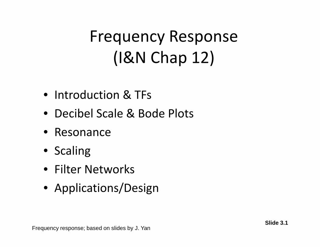
RC Circuit AC Response Letrsquos motivate this topic with a simple RC circuit example
If R=1Ω and C=1F determine the forced response
Time Domain Freq Domain
Input vs(t) Output vo(t) (steady-state)
cos(t) V
5cos(t-20ordm) V
1 V
cos(10t) V
cos(100t) V
Frequency response based on slides by J Yan
Slide 33
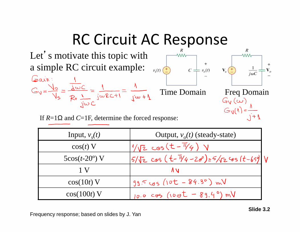
RC Example Comments bull From AC analysis if the input frequency is known only the
magnitude and phase of the output need to be computed
bull Using linearity and time-invariance only the magnitude gain and phase difference need to be computed This is evident when comparing the outputs to the 1st and 2nd inputs The gain in both cases is 2-frac12asymp0707 and the relative phase is -45ordm
bull Both the magnitude gain and phase difference vary with frequency For which frequency is the capacitor voltage identical to that of the source input and why
Frequency response based on slides by J Yan
Slide 34
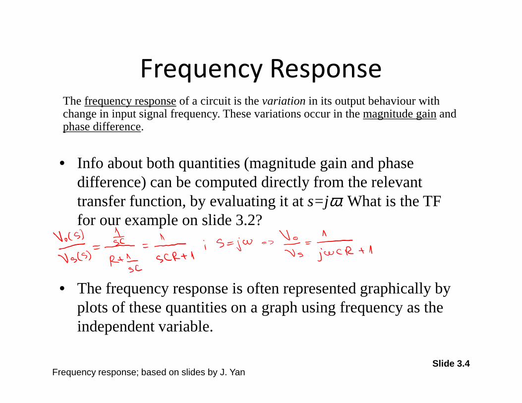
Frequency Response The frequency response of a circuit is the variation in its output behaviour with change in input signal frequency These variations occur in the magnitude gain and phase difference
bull Info about both quantities (magnitude gain and phase difference) can be computed directly from the relevant transfer function by evaluating it at s=jω What is the TF for our example on slide 32
bull The frequency response is often represented graphically by plots of these quantities on a graph using frequency as the independent variable
Frequency response based on slides by J Yan
Slide 35
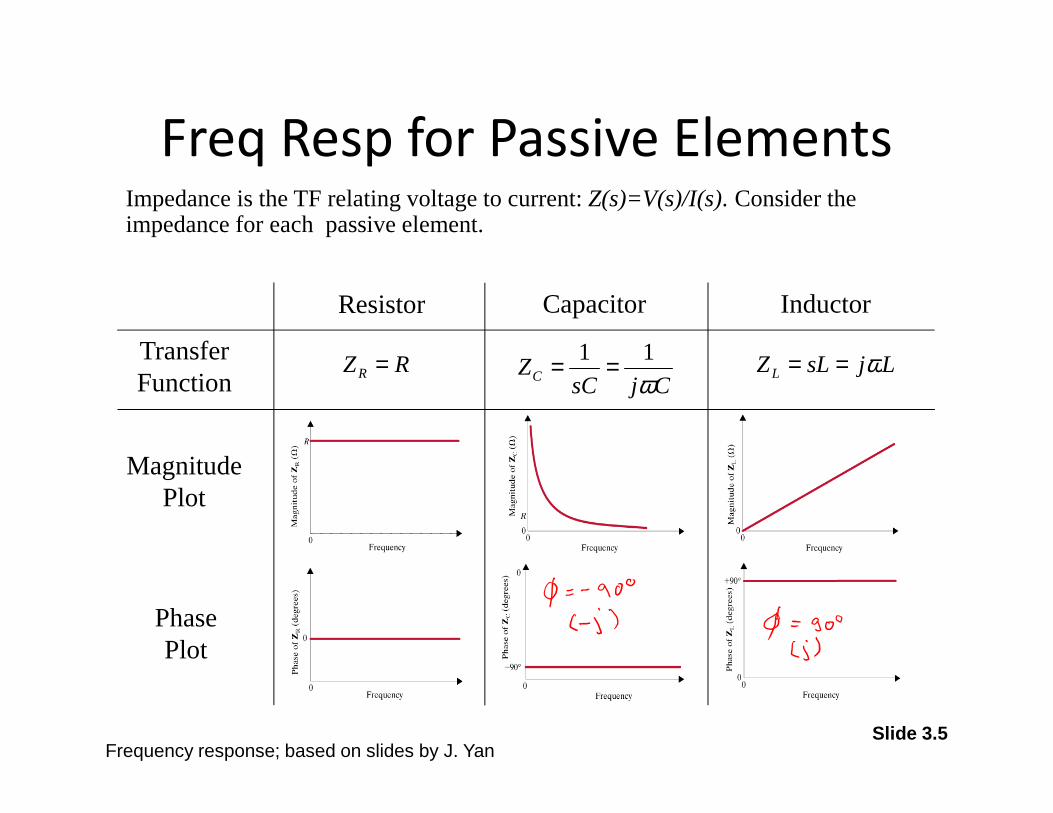
Freq Resp for Passive Elements
CjsCZC ω
11 == LjsLZL ω==RZR =Transfer Function
Magnitude Plot
Phase Plot
Resistor Capacitor Inductor
Impedance is the TF relating voltage to current Z(s)=V(s)I(s) Consider the impedance for each passive element
Frequency response based on slides by J Yan
Slide 36
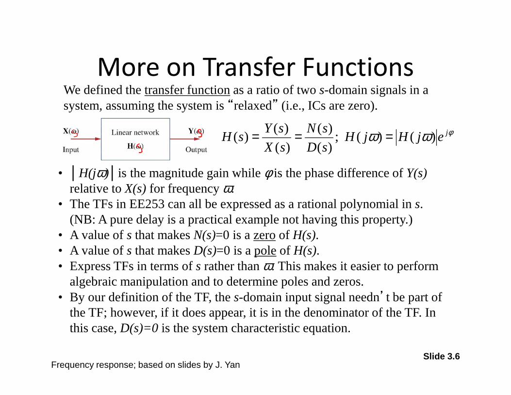
More on Transfer Functions We defined the transfer function as a ratio of two s-domain signals in a system assuming the system is ldquorelaxedrdquo (ie ICs are zero)
φωω jejHjHsD
sN
sX
sYsH )()(
)(
)(
)(
)()( ===
bull H(jω)is the magnitude gain while φ is the phase difference of Y(s)relative to X(s) for frequency ω
bull The TFs in EE253 can all be expressed as a rational polynomial in s (NB A pure delay is a practical example not having this property)
bull A value of s that makes N(s)=0 is a zero of H(s) bull A value of s that makes D(s)=0 is a pole of H(s) bull Express TFs in terms of s rather than ω This makes it easier to perform
algebraic manipulation and to determine poles and zerosbull By our definition of the TF the s-domain input signal neednrsquot be part of
the TF however if it does appear it is in the denominator of the TF In this case D(s)=0 is the system characteristic equation
Frequency response based on slides by J Yan
Slide 37
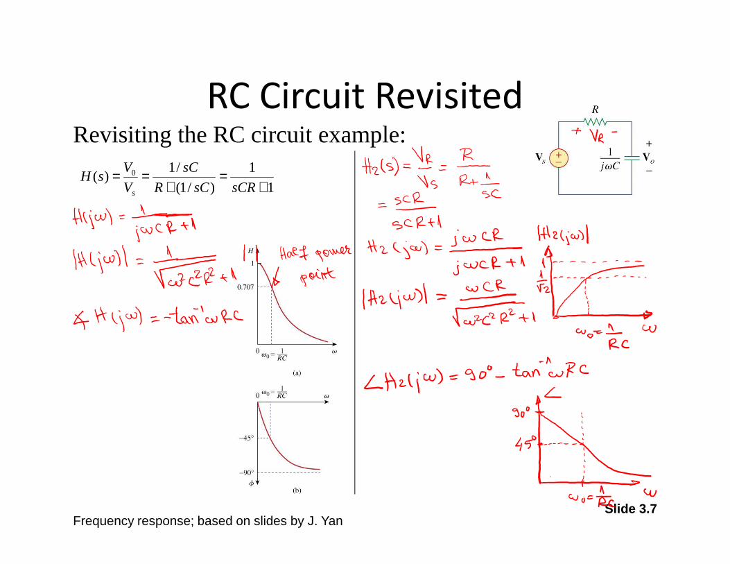
RC Circuit Revisited Revisiting the RC circuit example
1
1
)1(
1)( 0
+=
+==
sCRsCR
sC
V
VsH
s
Frequency response based on slides by J Yan
Slide 38
Example Find H(s)=Vo(s)Ii(s) the poles and zeros Sketch the freq resp
Frequency response based on slides by J Yan
Slide 39
Logarithm Properties
Logarithms will be used to more quickly and systematically sketch the frequency response graphs Itrsquos worthwhile to review a few of their properties
1 log(P1P2)=log(P1)+log(P2)2 log(P1P2)=log(P1)-log(P2)3 log(Pn)=nlog(P)4 log(01)=-1 log(1)=0 log(10)=1 log(100)=2 hellip
Frequency response based on slides by J Yan
Slide 310
Decibel ScaleHistorically the ldquogainrdquo G in communication systems was the ratio of power levels between 2 signals measured in bels (B)
The decibel (dB) is a tenth of a bel and is more convenient to use Since the power in a signal is proportional to the square of the voltage or to the square of the current
Frequency response based on slides by J Yan
Slide 311
Decibel Scale1 If power ratio is known use
10log(P2P1) If voltage or current ratio is known use 20log(V2V1) or 20log(I2I1)
bull Only the voltage or current magnitudes are used in the calculations Negative signs and angles are handled by the phase
bull When specifying the TF gain the dB absolute value is only meaningful for voltage or current gains
Magnitude H 20logH (dB)
0001
001
01
05
2-05
1
205
2
10
100
1000
Frequency response based on slides by J Yan
Slide 312
Bode Plots
)log())(log())(log(
)()(
ejjHjH
ejHjH j
times+=
=
φωωωω φ
Plotting the frequency response on a linear scale as done in slides 37 amp 38 is somewhat laborious In the late 1930s Hendrick W Bode developed standard Bode plots which take advantage of logarithm properties to allow for quick and easy plots that conveniently span a large frequency range
ωωφωω
log vs)( (semilog) sticCharacteri Phase
log vs)(log20 log)-(log sticCharacteri Magnitude
Plots Bode
jH
jHH dB
ang==
Frequency response based on slides by J Yan
Slide 313
( ) ( ) cpzszn
issn
is
n
issn
isN
n
i i
m
i i
nnn
mm
nnNms
K
ps
zsK
ssasaa
sbsbb
sD
sN
sX
sYsH
cpp
icppicpp
icppsp
ip
cpz
icpzicpz
icpzsz
iz 2 where1)1(
1)1(
)(
)(
)(
)(
)(
)()(
1
22
1
1
22
1
1
11
1110
10
++=+++
+++=
minus
minus=
+++++++==
=
prodprodprodprod
prodprod
==
==
=
=
minusminus
ωωζ
ω
ωωζ
ω
L
L
Transfer FunctionThe TF is commonly written in one of the following forms
Characteristicpolynomial
zeros
poles
of simple zeros
of zeros
of complex pairs of zeros
of zeros at origin(assumes Ngt0)
This form most convenient for frequency response plots (itrsquos not as ugly as it looks)
Frequency response based on slides by J Yan
Slide 314
Computation for Bode Diagram
Thus we have 4 types of terms to consider in the contribution to the magnitude and phase characteristics
( )( )prodprod
prodprod==
==
+++
+++=
cpp
icppicpp
icppsp
ip
cpz
icpzicpz
icpzsz
iz
n
issn
is
n
issn
isNs
KsH
1
2
1
1
2
1
2
2
2
2
1)1(
1)1()(
ωωζ
ω
ωωζ
ω
11
11loglog20)(log20
1
2
1
2
11
2
2
2
2
sumsum
sumsum
==
==
+minusminus+minus+
+minus+++==rArr
cpp
icpp
icpp
icpp
cpz
icpz
icpz
icpz
sp
ip
sz
iz
n
i
n
i
n
i
jn
i
jdB
jj
NKjHH
ωωζ
ωω
ωωζ
ωω
ωω
ωωωω L
tantan
tantan900 if 180
0 if 0
1
21
1
21
1
1
1
1
2222 sumsum
sumsum
= minusminus
= minusminus
=minus
=minus
minus+
minus+degsdot+
ltdegplusmngedeg
=rArr
cpp
icpp
icppicppcpz
icpz
icpzicpz
sp
ip
sz
iz
n
i
n
i
n
i
n
iN
K
K
ωω
ωωζ
ωω
ωωζ
ωω
ωωφ L
Frequency response based on slides by J Yan
Slide 315
Constant TermK
Frequency response based on slides by J Yan
Slide 316
PolesZeros at Origin
N poles at origin contribute -20N dBdecade to the magnitude (passing through 1 rads at 0 dB) and ndashN90degto the phase
N zeros at origin contribute 20N dBdecade to the magnitude (passing through 1 rads at 0 dB) and N90deg to the phase
( ) ( )( )
degtimesplusmn=
timesplusmn=rArr=
plusmn
plusmnplusmn
=
plusmn
90
)log(20
Njangle
Njjs
NdB
NN
js
N
ω
ωωω
ω
Frequency response based on slides by J Yan
Slide 317
Simple Zeros
degasymp+
asymp+rArrltlt
01
011 asymptote freq Low
i
i
i jdB
j
angle ωω
ωω
ωω
( ) ( )
=+
+=+rArr+=+
minus=ii
ii
ii jdB
jj
js
s
angle ωω
ωω
ωω
ωω
ωω
ωω 1
2
tan1
1log20111
degasymp+
asymp+rArrgtgt
901
log2011 asymptote freq Hi
i
ii
i jdB
j
angle ωω
ωω
ωω
ωω
Frequency response based on slides by J Yan
Slide 318
Simple Zeros
Magnitude characteristic approximated by 2 straight line asymptotes Horizontal line at 0dB ldquobreaks awayrdquo at ω=ωi with slope 20dBdecade At this corner or break frequency Where is this approximation worst and what is the error value
Phase characteristic approximated by 3 straight line segments 2 horizontal lines at 0deg and 90degconnected by 45degdecade line passing through ωi at 45deg
ω101ω1 10ω1
ω101ω1 10ω1
Frequency response based on slides by J Yan
Slide 319
ω
ω
Simple poles
( ) ( ) ( )( ) ( )
( )
minus=+
+minus=+rArr+=+=+
minusminus
minus
minusminus
=
minus
ii
ii
ii j
dB
j
ij
js
s
anglej
ωω
ωω
ωω
ωω
ωω
ωω ωτ11
21
111
tan1
1log201111
Itrsquos easy to see that the frequency response to a simple pole is the mirror image of that for a simple zero reflected across the ω axis
ω101ω1 10ω1
ω101ω1 10ω1
HdB
φ
Frequency response based on slides by J Yan
Slide 320
Quadratic Pole( ) ( )
( ) ( ) ( )( )
minus=+minus
+minusminus=+minusrArr
+minus=++
minusminusminus
minus
minus
=
minus
222
2
2
2
2
2
2
2
2
2
2112
22212
1212
tan1
1log201
11
ωωζωω
ωζω
ωω
ωζω
ωω
ωζω
ωω
ωζω
ωω
ωωωζ
n
n
nn
nnnn
nnnn
jangle
j
j
dB
js
ss
Frequency response based on slides by J Yan
Slide 321
Algorithm for Sketching Bode
Diagrams
( )( )prodprod
prodprod==
==
+++
+++=
cpp
icppicpp
icppsp
ip
cpz
icpzicpz
icpzsz
iz
n
issn
is
n
issn
isNs
KsH
1
2
1
1
2
1
2
2
2
2
1)1(
1)1()(
form standard in the Express 1 Step
ωωζ
ω
ωωζ
ω
Step 2 Use straight-line sketches to show the contribution to the magnitude and phase characteristics from each multiplicand
Step 3 Add lines together for complete frequency response
Frequency response based on slides by J Yan
Slide 322
Example
)10(
)2(5)(for plot Bode theDraw
++=
ss
ssH
10-1
100
101
102
103
-20
-10
0
10
20
Mag
nitu
de (
dB)
01 1 10 100 1000-90
-45
0
45
90
Pha
se (
deg)
Frequency response based on slides by J Yan
Slide 32
RC Circuit AC Response Letrsquos motivate this topic with a simple RC circuit example
If R=1Ω and C=1F determine the forced response
Time Domain Freq Domain
Input vs(t) Output vo(t) (steady-state)
cos(t) V
5cos(t-20ordm) V
1 V
cos(10t) V
cos(100t) V
Frequency response based on slides by J Yan
Slide 33
RC Example Comments bull From AC analysis if the input frequency is known only the
magnitude and phase of the output need to be computed
bull Using linearity and time-invariance only the magnitude gain and phase difference need to be computed This is evident when comparing the outputs to the 1st and 2nd inputs The gain in both cases is 2-frac12asymp0707 and the relative phase is -45ordm
bull Both the magnitude gain and phase difference vary with frequency For which frequency is the capacitor voltage identical to that of the source input and why
Frequency response based on slides by J Yan
Slide 34
Frequency Response The frequency response of a circuit is the variation in its output behaviour with change in input signal frequency These variations occur in the magnitude gain and phase difference
bull Info about both quantities (magnitude gain and phase difference) can be computed directly from the relevant transfer function by evaluating it at s=jω What is the TF for our example on slide 32
bull The frequency response is often represented graphically by plots of these quantities on a graph using frequency as the independent variable
Frequency response based on slides by J Yan
Slide 35
Freq Resp for Passive Elements
CjsCZC ω
11 == LjsLZL ω==RZR =Transfer Function
Magnitude Plot
Phase Plot
Resistor Capacitor Inductor
Impedance is the TF relating voltage to current Z(s)=V(s)I(s) Consider the impedance for each passive element
Frequency response based on slides by J Yan
Slide 36
More on Transfer Functions We defined the transfer function as a ratio of two s-domain signals in a system assuming the system is ldquorelaxedrdquo (ie ICs are zero)
φωω jejHjHsD
sN
sX
sYsH )()(
)(
)(
)(
)()( ===
bull H(jω)is the magnitude gain while φ is the phase difference of Y(s)relative to X(s) for frequency ω
bull The TFs in EE253 can all be expressed as a rational polynomial in s (NB A pure delay is a practical example not having this property)
bull A value of s that makes N(s)=0 is a zero of H(s) bull A value of s that makes D(s)=0 is a pole of H(s) bull Express TFs in terms of s rather than ω This makes it easier to perform
algebraic manipulation and to determine poles and zerosbull By our definition of the TF the s-domain input signal neednrsquot be part of
the TF however if it does appear it is in the denominator of the TF In this case D(s)=0 is the system characteristic equation
Frequency response based on slides by J Yan
Slide 37
RC Circuit Revisited Revisiting the RC circuit example
1
1
)1(
1)( 0
+=
+==
sCRsCR
sC
V
VsH
s
Frequency response based on slides by J Yan
Slide 38
Example Find H(s)=Vo(s)Ii(s) the poles and zeros Sketch the freq resp
Frequency response based on slides by J Yan
Slide 39
Logarithm Properties
Logarithms will be used to more quickly and systematically sketch the frequency response graphs Itrsquos worthwhile to review a few of their properties
1 log(P1P2)=log(P1)+log(P2)2 log(P1P2)=log(P1)-log(P2)3 log(Pn)=nlog(P)4 log(01)=-1 log(1)=0 log(10)=1 log(100)=2 hellip
Frequency response based on slides by J Yan
Slide 310
Decibel ScaleHistorically the ldquogainrdquo G in communication systems was the ratio of power levels between 2 signals measured in bels (B)
The decibel (dB) is a tenth of a bel and is more convenient to use Since the power in a signal is proportional to the square of the voltage or to the square of the current
Frequency response based on slides by J Yan
Slide 311
Decibel Scale1 If power ratio is known use
10log(P2P1) If voltage or current ratio is known use 20log(V2V1) or 20log(I2I1)
bull Only the voltage or current magnitudes are used in the calculations Negative signs and angles are handled by the phase
bull When specifying the TF gain the dB absolute value is only meaningful for voltage or current gains
Magnitude H 20logH (dB)
0001
001
01
05
2-05
1
205
2
10
100
1000
Frequency response based on slides by J Yan
Slide 312
Bode Plots
)log())(log())(log(
)()(
ejjHjH
ejHjH j
times+=
=
φωωωω φ
Plotting the frequency response on a linear scale as done in slides 37 amp 38 is somewhat laborious In the late 1930s Hendrick W Bode developed standard Bode plots which take advantage of logarithm properties to allow for quick and easy plots that conveniently span a large frequency range
ωωφωω
log vs)( (semilog) sticCharacteri Phase
log vs)(log20 log)-(log sticCharacteri Magnitude
Plots Bode
jH
jHH dB
ang==
Frequency response based on slides by J Yan
Slide 313
( ) ( ) cpzszn
issn
is
n
issn
isN
n
i i
m
i i
nnn
mm
nnNms
K
ps
zsK
ssasaa
sbsbb
sD
sN
sX
sYsH
cpp
icppicpp
icppsp
ip
cpz
icpzicpz
icpzsz
iz 2 where1)1(
1)1(
)(
)(
)(
)(
)(
)()(
1
22
1
1
22
1
1
11
1110
10
++=+++
+++=
minus
minus=
+++++++==
=
prodprodprodprod
prodprod
==
==
=
=
minusminus
ωωζ
ω
ωωζ
ω
L
L
Transfer FunctionThe TF is commonly written in one of the following forms
Characteristicpolynomial
zeros
poles
of simple zeros
of zeros
of complex pairs of zeros
of zeros at origin(assumes Ngt0)
This form most convenient for frequency response plots (itrsquos not as ugly as it looks)
Frequency response based on slides by J Yan
Slide 314
Computation for Bode Diagram
Thus we have 4 types of terms to consider in the contribution to the magnitude and phase characteristics
( )( )prodprod
prodprod==
==
+++
+++=
cpp
icppicpp
icppsp
ip
cpz
icpzicpz
icpzsz
iz
n
issn
is
n
issn
isNs
KsH
1
2
1
1
2
1
2
2
2
2
1)1(
1)1()(
ωωζ
ω
ωωζ
ω
11
11loglog20)(log20
1
2
1
2
11
2
2
2
2
sumsum
sumsum
==
==
+minusminus+minus+
+minus+++==rArr
cpp
icpp
icpp
icpp
cpz
icpz
icpz
icpz
sp
ip
sz
iz
n
i
n
i
n
i
jn
i
jdB
jj
NKjHH
ωωζ
ωω
ωωζ
ωω
ωω
ωωωω L
tantan
tantan900 if 180
0 if 0
1
21
1
21
1
1
1
1
2222 sumsum
sumsum
= minusminus
= minusminus
=minus
=minus
minus+
minus+degsdot+
ltdegplusmngedeg
=rArr
cpp
icpp
icppicppcpz
icpz
icpzicpz
sp
ip
sz
iz
n
i
n
i
n
i
n
iN
K
K
ωω
ωωζ
ωω
ωωζ
ωω
ωωφ L
Frequency response based on slides by J Yan
Slide 315
Constant TermK
Frequency response based on slides by J Yan
Slide 316
PolesZeros at Origin
N poles at origin contribute -20N dBdecade to the magnitude (passing through 1 rads at 0 dB) and ndashN90degto the phase
N zeros at origin contribute 20N dBdecade to the magnitude (passing through 1 rads at 0 dB) and N90deg to the phase
( ) ( )( )
degtimesplusmn=
timesplusmn=rArr=
plusmn
plusmnplusmn
=
plusmn
90
)log(20
Njangle
Njjs
NdB
NN
js
N
ω
ωωω
ω
Frequency response based on slides by J Yan
Slide 317
Simple Zeros
degasymp+
asymp+rArrltlt
01
011 asymptote freq Low
i
i
i jdB
j
angle ωω
ωω
ωω
( ) ( )
=+
+=+rArr+=+
minus=ii
ii
ii jdB
jj
js
s
angle ωω
ωω
ωω
ωω
ωω
ωω 1
2
tan1
1log20111
degasymp+
asymp+rArrgtgt
901
log2011 asymptote freq Hi
i
ii
i jdB
j
angle ωω
ωω
ωω
ωω
Frequency response based on slides by J Yan
Slide 318
Simple Zeros
Magnitude characteristic approximated by 2 straight line asymptotes Horizontal line at 0dB ldquobreaks awayrdquo at ω=ωi with slope 20dBdecade At this corner or break frequency Where is this approximation worst and what is the error value
Phase characteristic approximated by 3 straight line segments 2 horizontal lines at 0deg and 90degconnected by 45degdecade line passing through ωi at 45deg
ω101ω1 10ω1
ω101ω1 10ω1
Frequency response based on slides by J Yan
Slide 319
ω
ω
Simple poles
( ) ( ) ( )( ) ( )
( )
minus=+
+minus=+rArr+=+=+
minusminus
minus
minusminus
=
minus
ii
ii
ii j
dB
j
ij
js
s
anglej
ωω
ωω
ωω
ωω
ωω
ωω ωτ11
21
111
tan1
1log201111
Itrsquos easy to see that the frequency response to a simple pole is the mirror image of that for a simple zero reflected across the ω axis
ω101ω1 10ω1
ω101ω1 10ω1
HdB
φ
Frequency response based on slides by J Yan
Slide 320
Quadratic Pole( ) ( )
( ) ( ) ( )( )
minus=+minus
+minusminus=+minusrArr
+minus=++
minusminusminus
minus
minus
=
minus
222
2
2
2
2
2
2
2
2
2
2112
22212
1212
tan1
1log201
11
ωωζωω
ωζω
ωω
ωζω
ωω
ωζω
ωω
ωζω
ωω
ωωωζ
n
n
nn
nnnn
nnnn
jangle
j
j
dB
js
ss
Frequency response based on slides by J Yan
Slide 321
Algorithm for Sketching Bode
Diagrams
( )( )prodprod
prodprod==
==
+++
+++=
cpp
icppicpp
icppsp
ip
cpz
icpzicpz
icpzsz
iz
n
issn
is
n
issn
isNs
KsH
1
2
1
1
2
1
2
2
2
2
1)1(
1)1()(
form standard in the Express 1 Step
ωωζ
ω
ωωζ
ω
Step 2 Use straight-line sketches to show the contribution to the magnitude and phase characteristics from each multiplicand
Step 3 Add lines together for complete frequency response
Frequency response based on slides by J Yan
Slide 322
Example
)10(
)2(5)(for plot Bode theDraw
++=
ss
ssH
10-1
100
101
102
103
-20
-10
0
10
20
Mag
nitu
de (
dB)
01 1 10 100 1000-90
-45
0
45
90
Pha
se (
deg)
Frequency response based on slides by J Yan
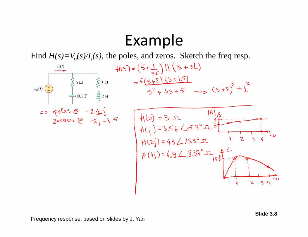
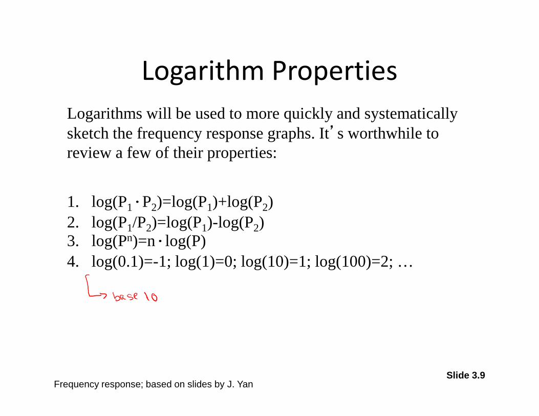
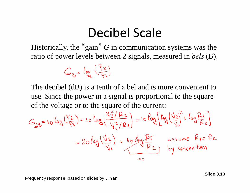
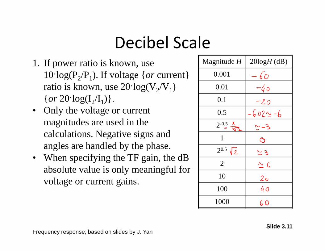
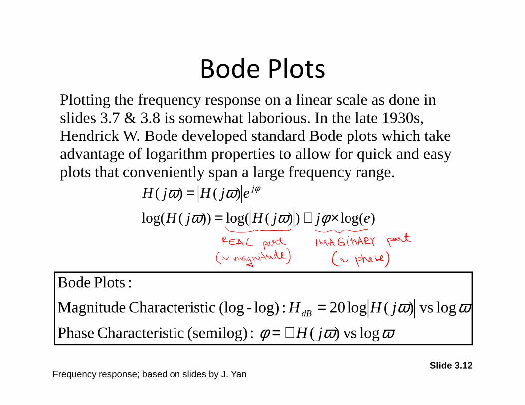
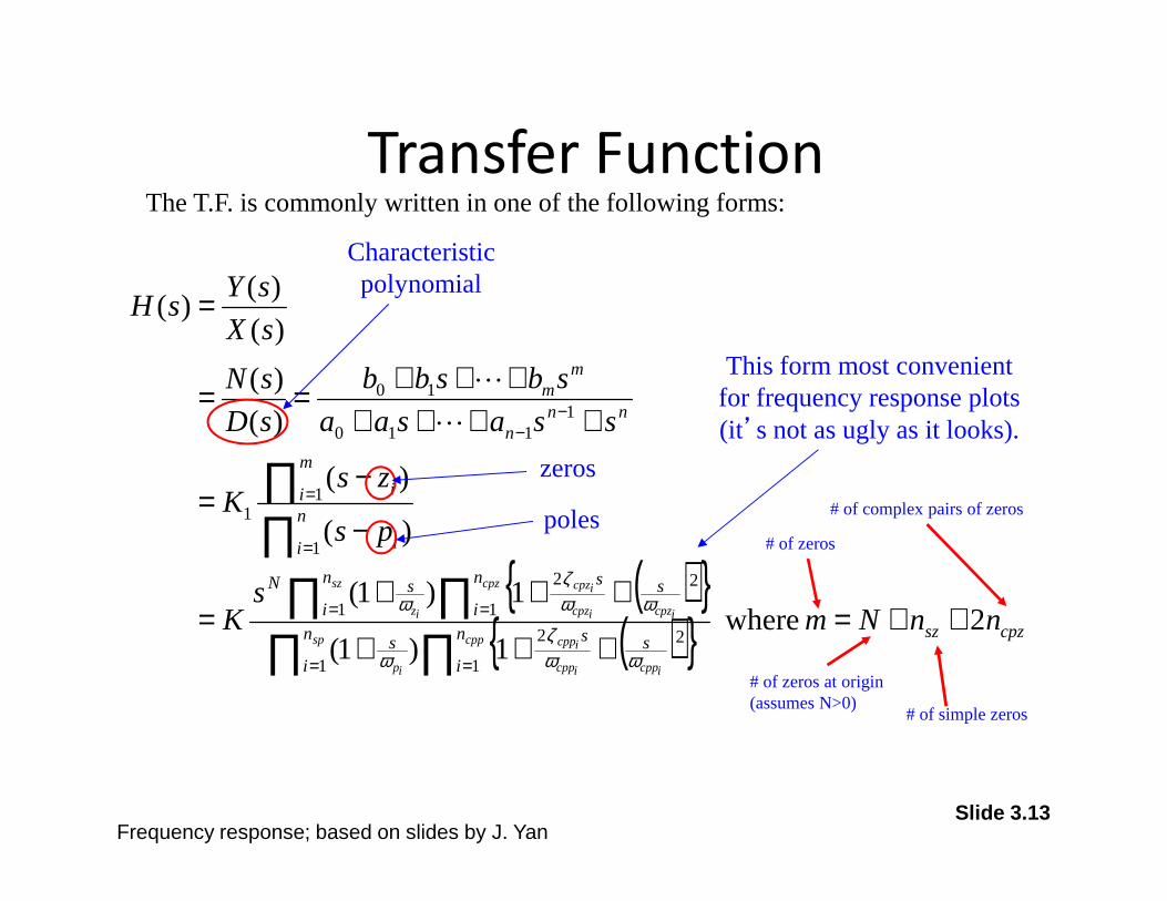
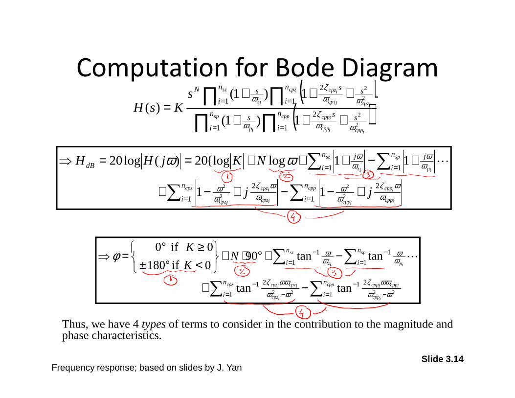
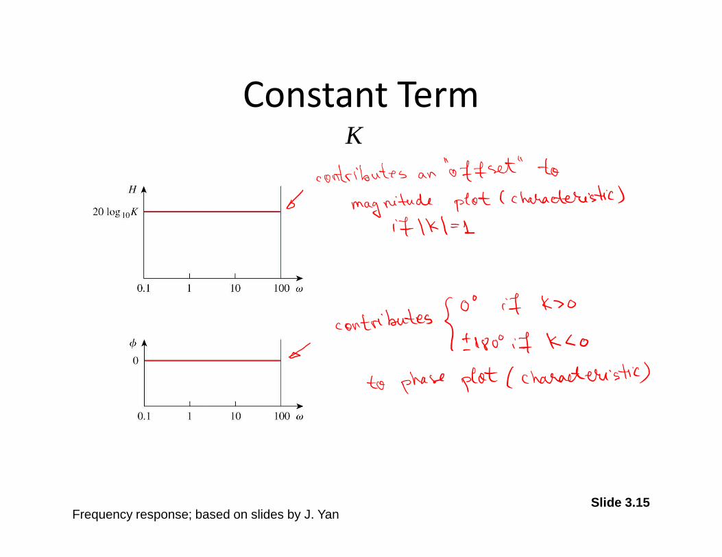
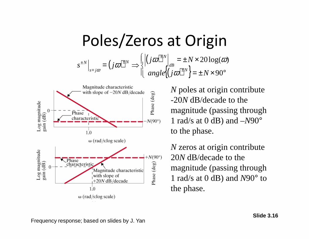
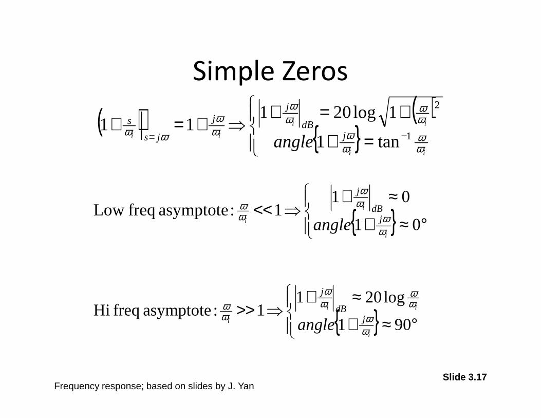
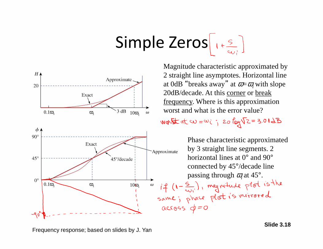
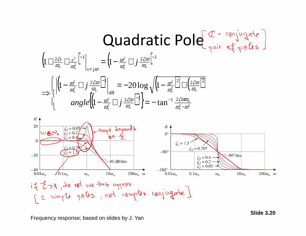
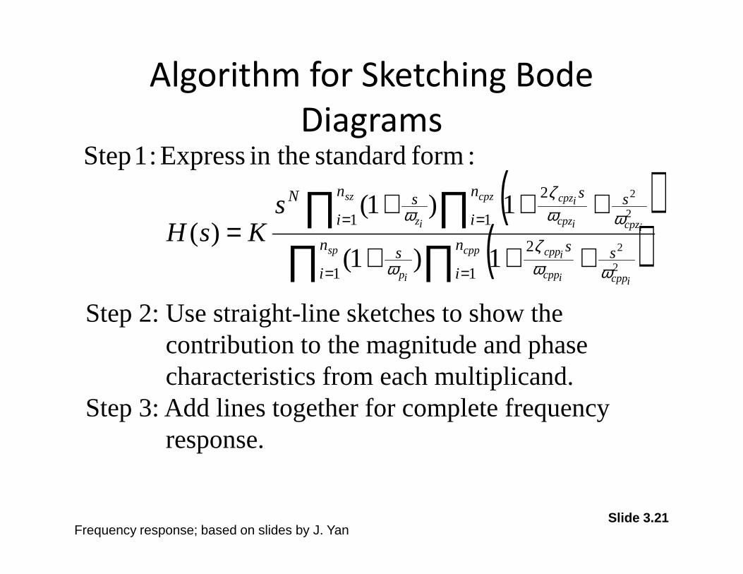

Slide 322
Example
)10(
)2(5)(for plot Bode theDraw
++=
ss
ssH
10-1
100
101
102
103
-20
-10
0
10
20
Mag
nitu
de (
dB)
01 1 10 100 1000-90
-45
0
45
90
Pha
se (
deg)
Frequency response based on slides by J Yan