1

Cha

pter

13

Frequency Response AnalysisSinusoidal Forcing of a First-Order ProcessFor a first-order transfer function with gain K and time constant , the response to a general sinusoidal input, is:

τ( ) sinω=x t A t

( ) ( )/ τ2 2 ωτ ωτcosω sinω (5-25)

ω τ 1−= − +

+tKAy t e t t

Note that y(t) and x(t) are in deviation form. The long-time response, yl(t), can be written as:

( ) ( )2 2

sin ω φ for (13-1)ω τ 1

= + →∞+

KAy t t t

( )1φ tan ωτ−= −where:

2

Cha

pter

13

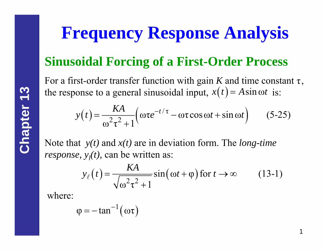
Figure 13.1 Attenuation and time shift between input and output sine waves (K= 1). The phase angle of the output signal is given by , where is the (period) shift and Pis the period of oscillation.

φφ Time shift / 360= − ×P t∆

3

Cha

pter

13

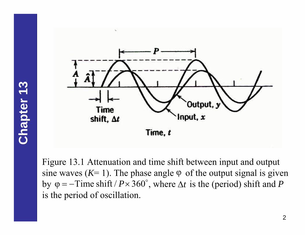
1. The output signal is a sinusoid that has the same frequency, ω,as the input.signal, x(t) =Asinωt.

2. The amplitude of the output signal, , is a function of the frequency ω and the input amplitude, A:

A

2 2ˆ (13-2)

ω τ 1=

+

KAA

Frequency Response Characteristics ofa First-Order Process

3. The output has a phase shift, φ, relative to the input. The amount of phase shift depends on ω.

( ) ( )ˆFor ( ) sin , sin ω φ as where :ω= = + →∞x t A t y t A t t

( )12 2

ˆ and φ tan ωτω τ 1

−= = −+

KAA

4

Cha

pter

13

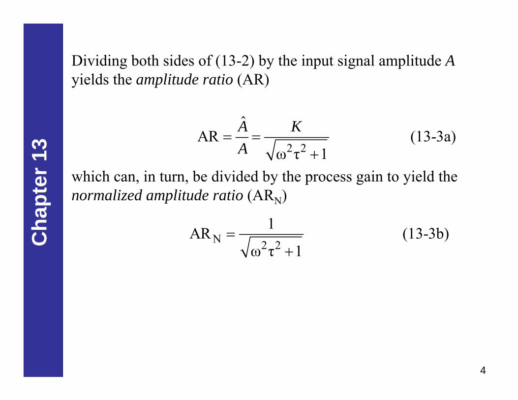
which can, in turn, be divided by the process gain to yield the normalized amplitude ratio (ARN)

N 2 2

1AR (13-3b)ω τ 1

=+

Dividing both sides of (13-2) by the input signal amplitude Ayields the amplitude ratio (AR)

2 2

ˆAR (13-3a)

ω τ 1= =

+

A KA

5

Cha

pter

13

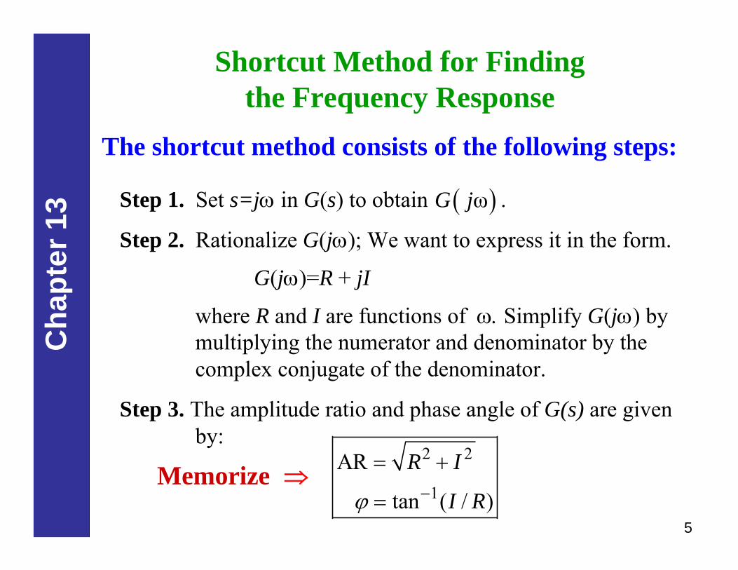
Shortcut Method for Finding the Frequency Response

The shortcut method consists of the following steps:

Step 1. Set s=jω in G(s) to obtain .

Step 2. Rationalize G(jω); We want to express it in the form.

G(jω)=R + jI

where R and I are functions of ω. Simplify G(jω) by multiplying the numerator and denominator by the complex conjugate of the denominator.

Step 3. The amplitude ratio and phase angle of G(s) are given by:

( )ωG j

2 2

1

AR

tan ( / )

R I

I Rϕ −

= +

=Memorize ⇒

6

Cha

pter

13

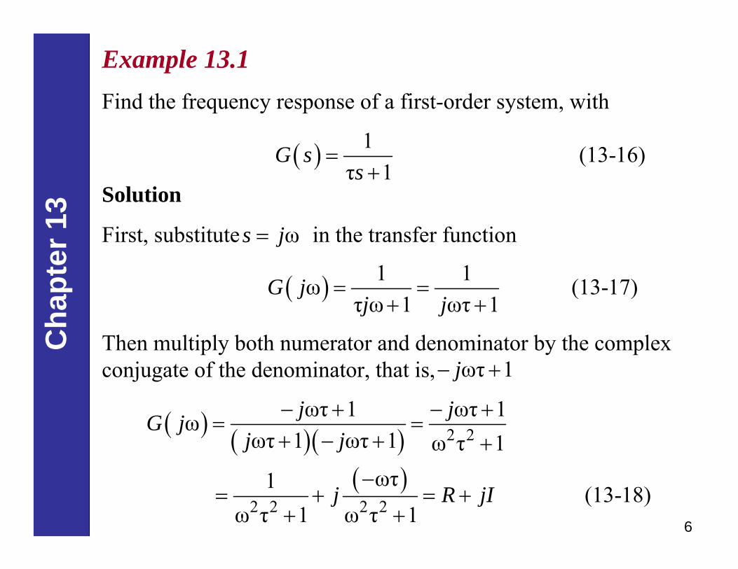
Example 13.1Find the frequency response of a first-order system, with

( ) 1 (13-16)τ 1

G ss

=+

Solution

First, substitute in the transfer functionωs j=

( ) 1 1ω (13-17)τ ω 1 ωτ 1

G jj j

= =+ +

Then multiply both numerator and denominator by the complex conjugate of the denominator, that is, ωτ 1j− +

( ) ( )( )( )

2 2

2 2 2 2

ωτ 1 ωτ 1ωωτ 1 ωτ 1 ω τ 1

ωτ1 (13-18)ω τ 1 ω τ 1

j jG jj j

j R jI

− + − += =

+ − + +

−= + = +

+ +

7

Cha

pter

13

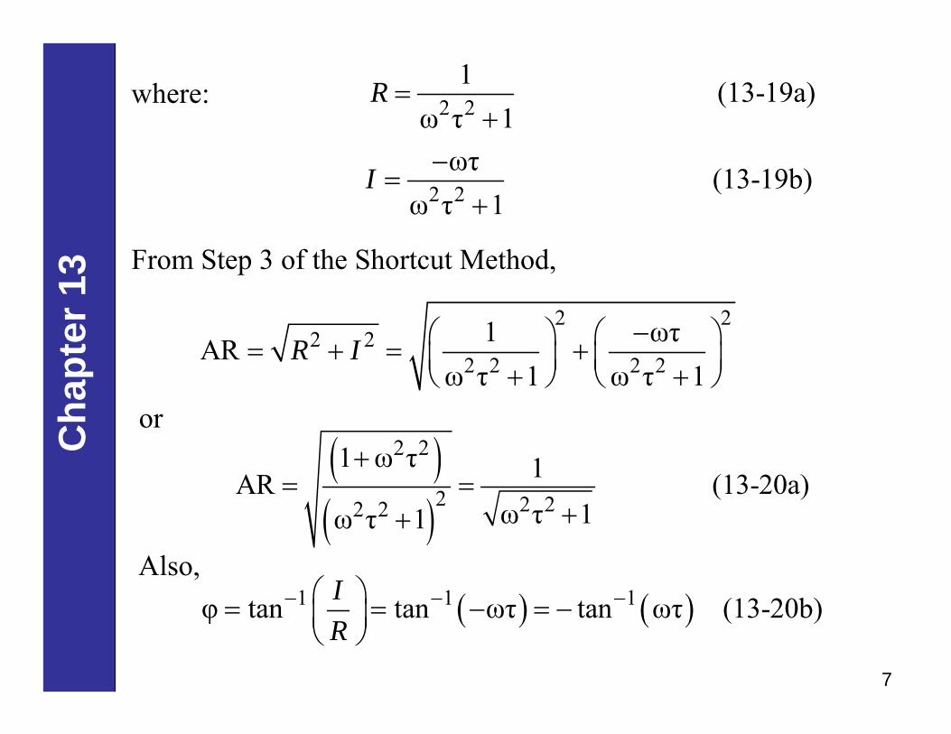
where:

From Step 3 of the Shortcut Method,

2 21 (13-19a)

ω τ 1R =

+

2 2ωτ (13-19b)

ω τ 1I −=

+

2 22 2

2 2 2 21 ωτAR

ω τ 1 ω τ 1−⎛ ⎞ ⎛ ⎞= + = +⎜ ⎟ ⎜ ⎟+ +⎝ ⎠ ⎝ ⎠

R I

( )( )

2 2

2 2 22 2

1 ω τ 1AR (13-20a)ω τ 1ω τ 1

+= =

++

or

Also,( ) ( )1 1 1φ tan tan ωτ tan ωτ (13-20b)− − −⎛ ⎞= = − = −⎜ ⎟

⎝ ⎠IR

8

Cha

pter

13

Consider a complex transfer G(s),

( ) ( ) ( ) ( )( ) ( ) ( )1 2 3

ω ω ωω (13-23)

ω ω ω= a b cG j G j G j

G jG j G j G j

From complex variable theory, we can express the magnitude and angle of as follows: ( )ωG j

( )( ) ( ) ( )( ) ( ) ( )1 2 3

ω ω ωω (13-24a)

ω ω ω= a b cG j G j G j

G jG j G j G j

( ) ( ) ( ) ( )( ) ( ) ( )1 2 3

ω ω ω ω

[ ω ω ω ] (13-24b)a b cG j G j G j G j

G j G j G j

∠ = ∠ +∠ +∠ +

− ∠ +∠ +∠ +

Complex Transfer Functions

( ) ( ) ( ) ( )( ) ( ) ( )1 2 3

(13-22)= a b cG s G s G sG s

G s G s G sSubstitute s=jω,

9

Cha

pter

13

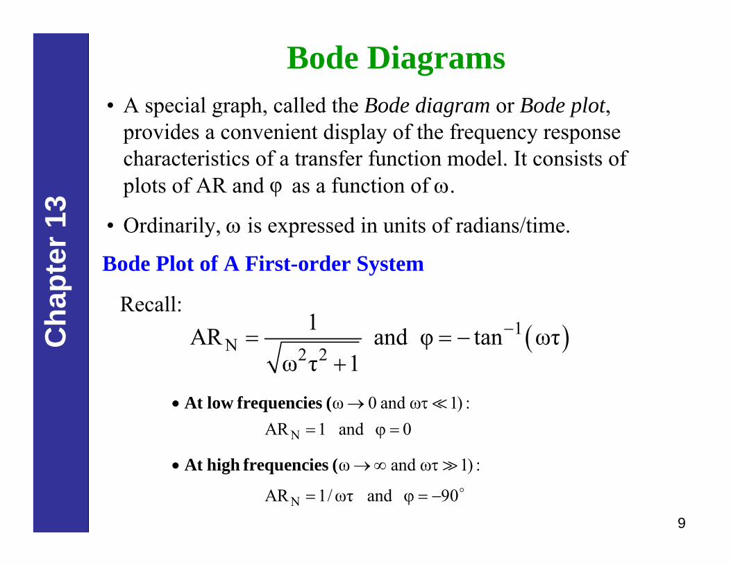
Bode Diagrams• A special graph, called the Bode diagram or Bode plot,

provides a convenient display of the frequency response characteristics of a transfer function model. It consists of plots of AR and as a function of ω.

• Ordinarily, ω is expressed in units of radians/time.

φ

Bode Plot of A First-order System

( )1N 2 2

1AR and φ tan ωτω τ 1

−= = −+

Recall:

N

N

ω 0 and ω 1) :AR 1 and

ω and ω 1) :

AR 1/ωτ and

• → τ= ϕ = 0

• →∞ τ

= ϕ = −90

At low frequencies (

At high frequencies (

10

Cha

pter

13

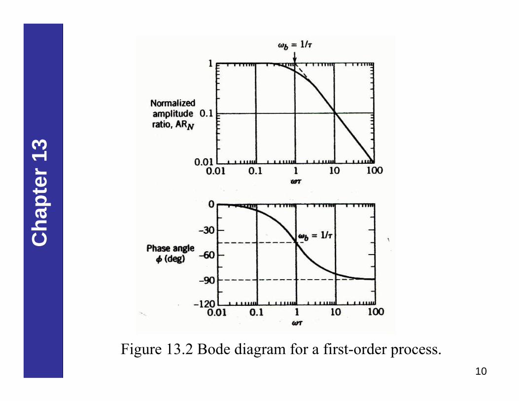
Figure 13.2 Bode diagram for a first-order process.

11

Cha

pter

13

• Note that the asymptotes intersect at , known as the break frequency or corner frequency. Here the value of ARNfrom (13-21) is:

ω ω 1/ τb= =

( )N1AR ω ω 0.707 (13-30)

1 1b= = =+

• Some books and software defined AR differently, in terms of decibels. The amplitude ratio in decibels ARd is defined as

dAR 20 log AR (13-33)=

12

Cha

pter

13

Integrating ElementsThe transfer function for an integrating element was given in Chapter 5:

( ) ( )( )

(5-34)Y s KG sU s s

= =

( )AR ω (13-34)ω ω

K KG jj

= = =

( ) ( )φ ω 90 (13-35)G j K= ∠ = ∠ −∠ ∞ = −

Second-Order ProcessA general transfer function that describes any underdamped, critically damped, or overdamped second-order system is

( ) 2 2 (13-40)τ 2ζτ 1

KG ss s

=+ +

13

Cha

pter

13

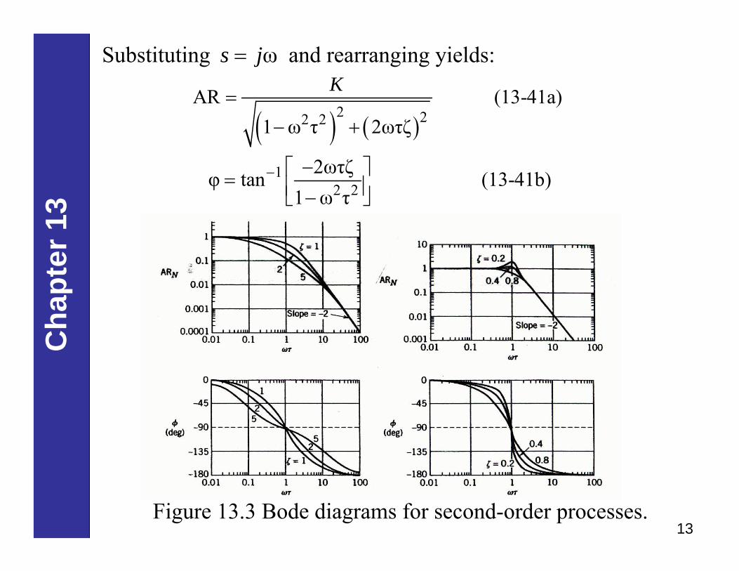
Substituting and rearranging yields:ωs j=

( ) ( )2 22 2

AR (13-41a)1 ω τ 2ωτζ

K=

− +

12 2

2ωτζφ tan (13-41b)1 ω τ

− −⎡ ⎤= ⎢ ⎥−⎣ ⎦

Figure 13.3 Bode diagrams for second-order processes.

14

Cha

pter

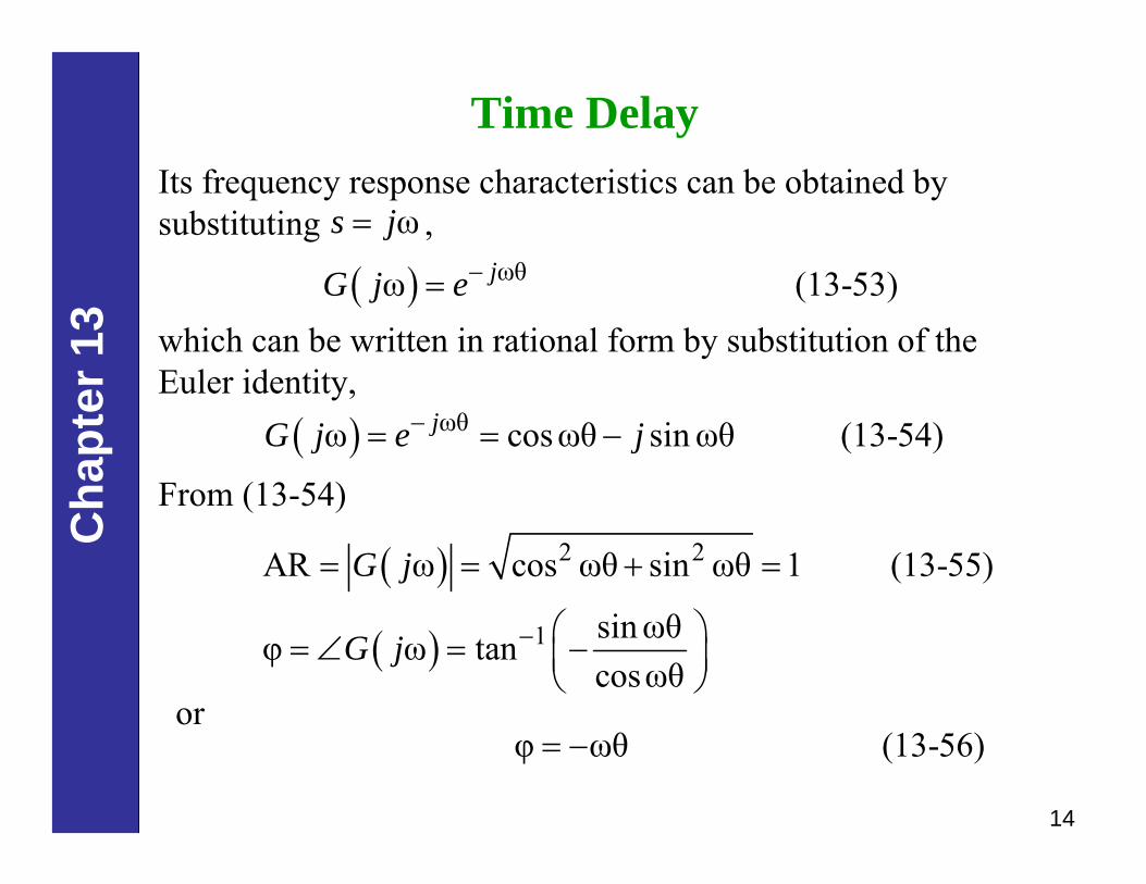
13 which can be written in rational form by substitution of the

Euler identity,( ) ωθω cosωθ sinωθ (13-54)−= = −jG j e j

From (13-54)

( )

( )

2 2

1

AR ω cos ωθ sin ωθ 1 (13-55)

sinωθφ ω tancosωθ

G j

G j −

= = + =

⎛ ⎞= ∠ = −⎜ ⎟⎝ ⎠

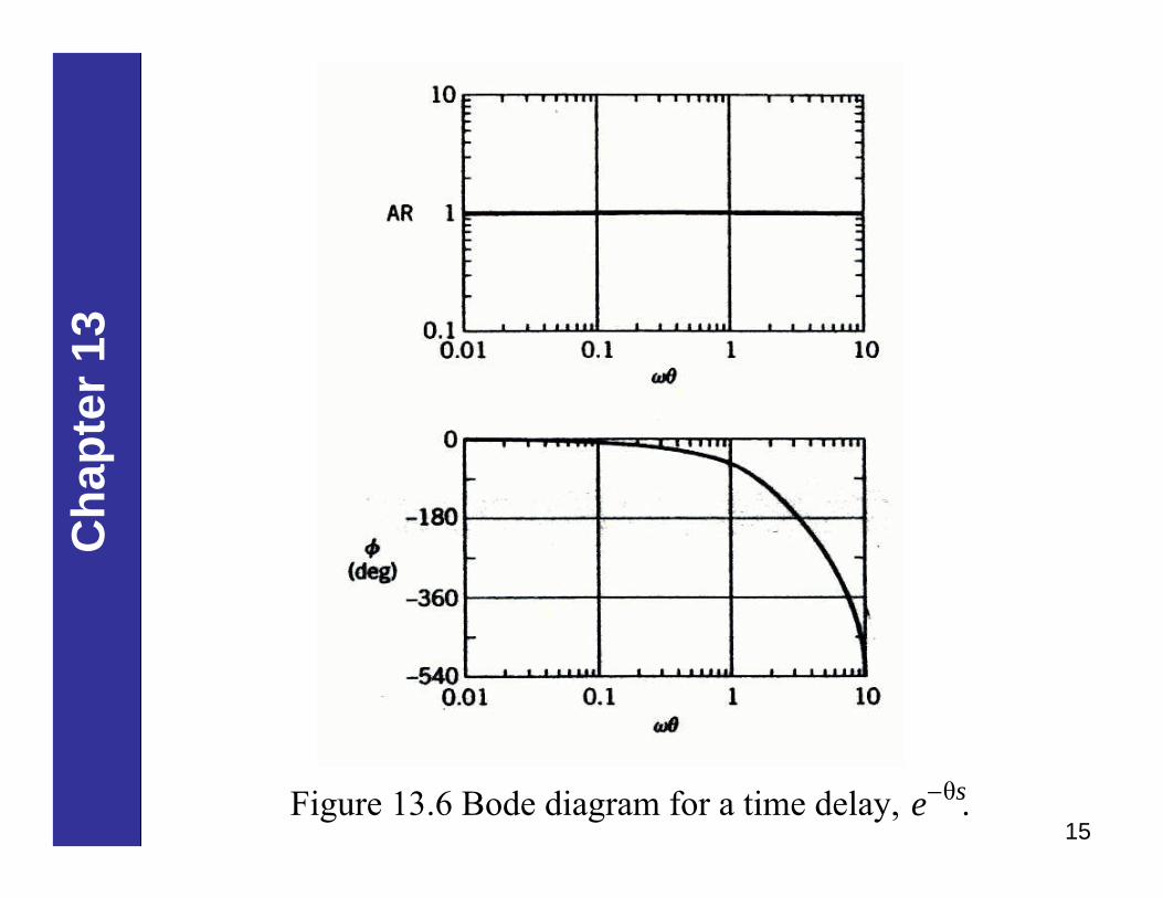
orφ ωθ (13-56)= −

Time DelayIts frequency response characteristics can be obtained by substituting , ωs j=

( ) ωθω (13-53)jG j e−=

15

Cha

pter

13

Figure 13.6 Bode diagram for a time delay, .θse−

16

Cha

pter

13

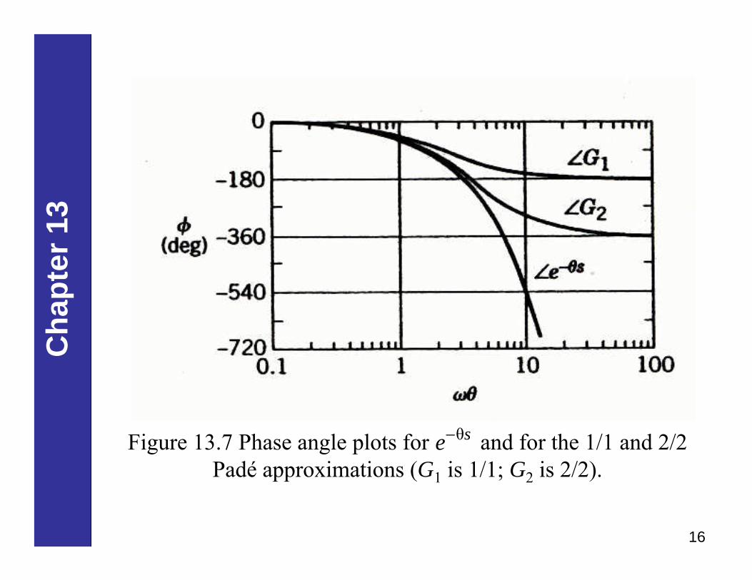
Figure 13.7 Phase angle plots for and for the 1/1 and 2/2 Padé approximations (G1 is 1/1; G2 is 2/2).

θse−

17

Cha

pter

13

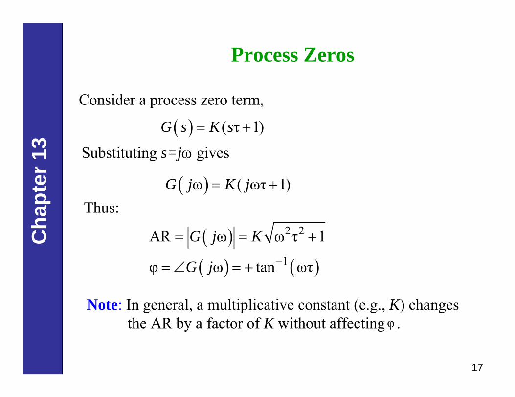
( )ω ( ωτ 1)= +G j K j

( )( ) ( )

2 2

1

AR ω ω τ 1

φ ω tan ωτ−

= = +

= ∠ = +

G j K

G j

Process Zeros

Substituting s=jω gives

Consider a process zero term,

( ) ( τ 1)= +G s K s

Thus:

Note: In general, a multiplicative constant (e.g., K) changes the AR by a factor of K without affecting .φ

18

Cha

pter

13

Frequency Response Characteristics of Feedback Controllers

Proportional Controller. Consider a proportional controller with positive gain

( ) (13-57)c cG s K=

In this case , which is independent of ω. Therefore,

( )ωc cG j K=

AR (13-58)c cK=

and φ 0 (13-59)c =

19

Cha

pter

13

Proportional-Integral Controller. A proportional-integral (PI) controller has the transfer function (cf. Eq. 8-9),

( ) τ 111 (13-60)τ τ

Ic c c

I I

sG s K Ks s

⎛ ⎞ ⎛ ⎞+= + =⎜ ⎟ ⎜ ⎟

⎝ ⎠ ⎝ ⎠

Thus, the amplitude ratio and phase angle are:

( )( )

( )22

ωτ 11AR ω 1 (13-62)ωτωτ

Ic c c c

II

G j K K+

= = + =

( ) ( ) ( )1 1φ ω tan 1/ωτ tan ωτ 90 (13-63)c c I IG j − −= ∠ = − = −

Substitute s=jω:

( ) τ 11 11 1τ τ τ

⎛ ⎞ ⎛ ⎞ ⎛ ⎞ω +ω = + = = −⎜ ⎟ ⎜ ⎟ ⎜ ⎟ω ω ω⎝ ⎠ ⎝ ⎠ ⎝ ⎠

Ic c c c

I I I

jG j K K K jj j

20

Cha

pter

13

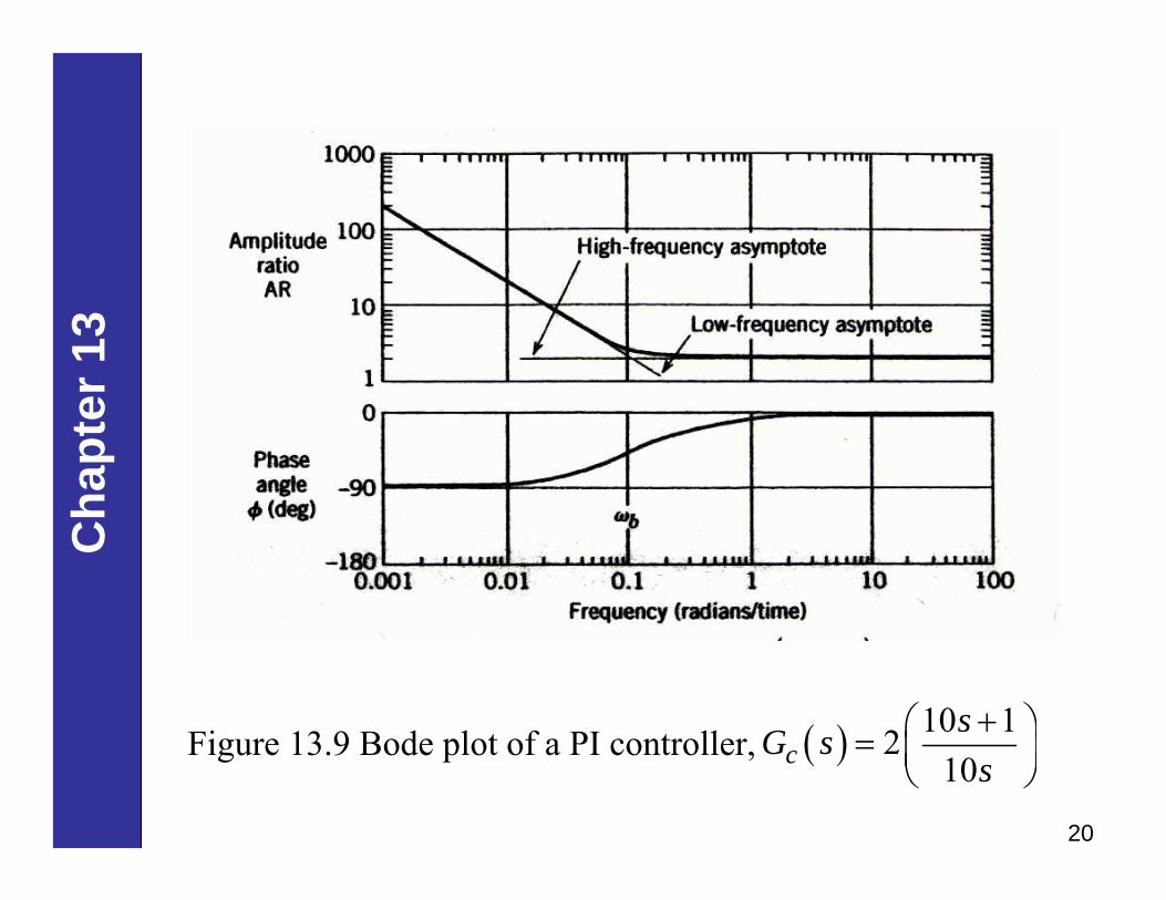
Figure 13.9 Bode plot of a PI controller, ( ) 10 1210csG s

s+⎛ ⎞= ⎜ ⎟

⎝ ⎠

21

Cha

pter

13

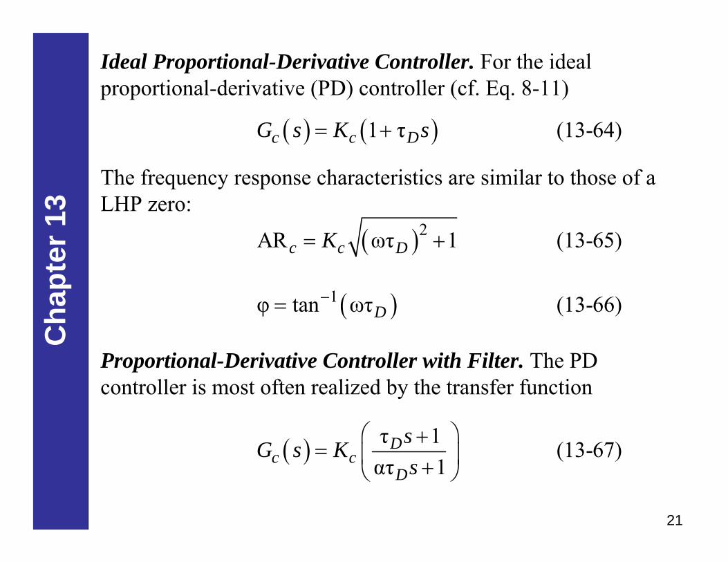
Ideal Proportional-Derivative Controller. For the ideal proportional-derivative (PD) controller (cf. Eq. 8-11)

The frequency response characteristics are similar to those of aLHP zero:

( ) ( )1 τ (13-64)c c DG s K s= +

( )2AR ωτ 1 (13-65)c c DK= +

( )1φ tan ωτ (13-66)D−=

Proportional-Derivative Controller with Filter. The PD controller is most often realized by the transfer function

( ) τ 1 (13-67)ατ 1

Dc c

D

sG s Ks

⎛ ⎞+= ⎜ ⎟+⎝ ⎠

22

Cha

pter

13

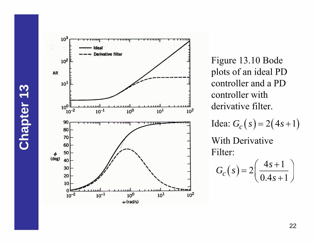
Figure 13.10 Bode plots of an ideal PD controller and a PD controller with derivative filter.

Idea:

With Derivative Filter:

( ) 4 120.4 1c

sG ss+⎛ ⎞= ⎜ ⎟+⎝ ⎠

( ) ( )2 4 1cG s s= +

23

Cha

pter

13

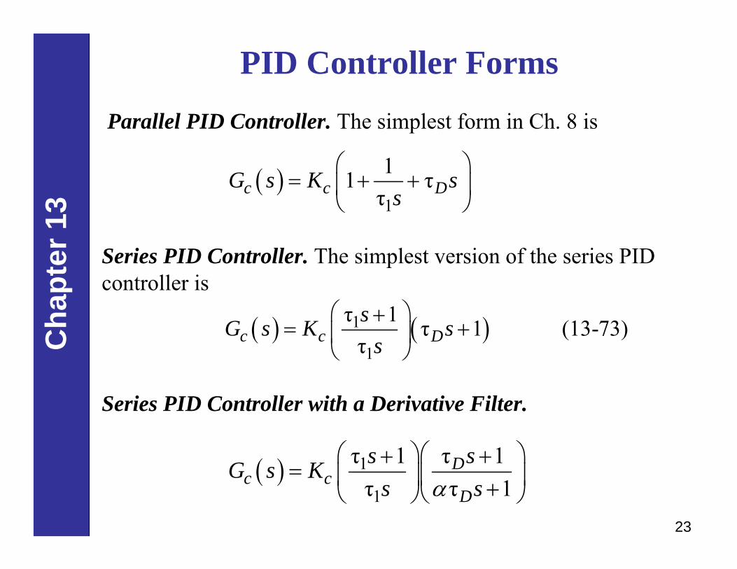
Series PID Controller. The simplest version of the series PID controller is

Series PID Controller with a Derivative Filter.

( ) ( )1

1

τ 1 τ 1 (13-73)τc c DsG s K s

s⎛ ⎞+

= +⎜ ⎟⎝ ⎠

PID Controller FormsParallel PID Controller. The simplest form in Ch. 8 is

( )1

11 ττc c DG s K s

s⎛ ⎞

= + +⎜ ⎟⎝ ⎠

( ) 1

1

τ 1 τ 1τ τ 1

Dc c

D

s sG s Ks sα

⎛ ⎞⎛ ⎞+ += ⎜ ⎟⎜ ⎟+⎝ ⎠⎝ ⎠

24

Cha

pter

13

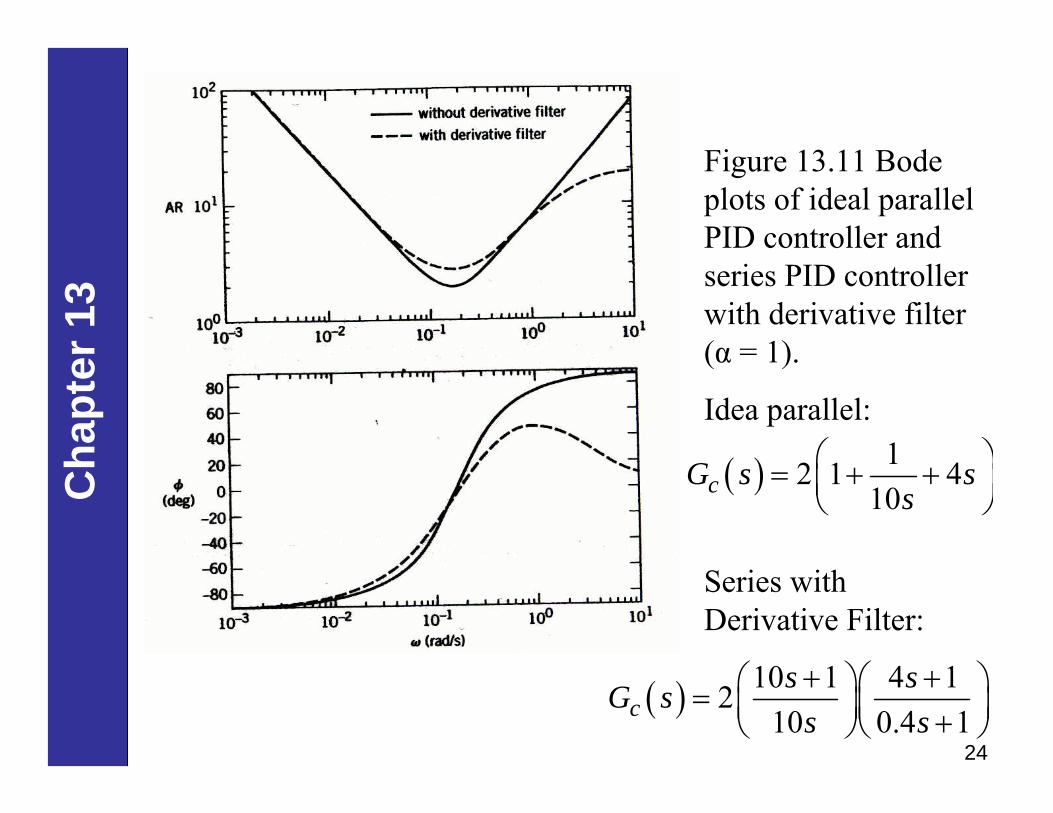
Figure 13.11 Bode plots of ideal parallel PID controller and series PID controller with derivative filter (α = 1).

Idea parallel:

Series with Derivative Filter:

( ) 10 1 4 1210 0.4 1cs sG s

s s+ +⎛ ⎞⎛ ⎞= ⎜ ⎟⎜ ⎟+⎝ ⎠⎝ ⎠

( ) 12 1 410cG s s

s⎛ ⎞= + +⎜ ⎟⎝ ⎠

25

Cha

pter

13

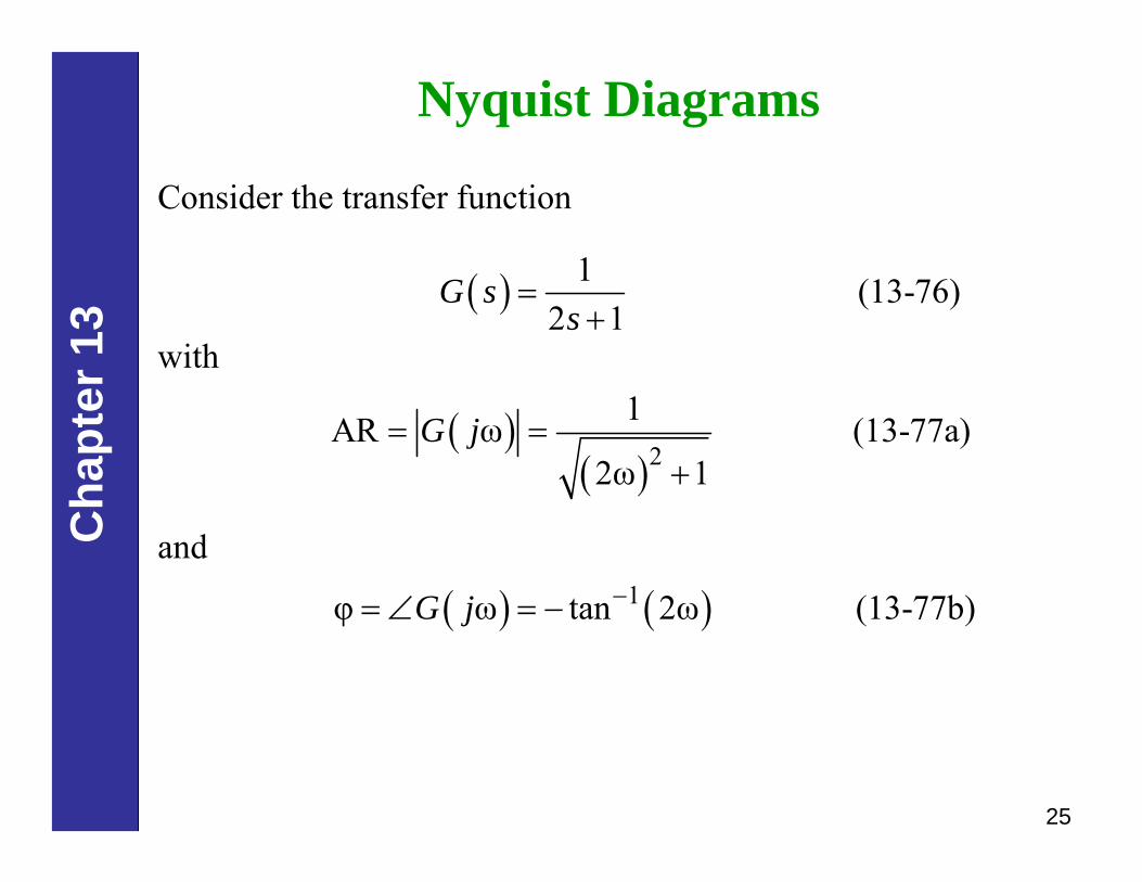
Nyquist Diagrams

Consider the transfer function

( ) 1 (13-76)2 1

G ss

=+

with

( )( )2

1AR ω (13-77a)2ω 1

G j= =+

and

( ) ( )1φ ω tan 2ω (13-77b)G j −= ∠ = −

26

Cha

pter

13

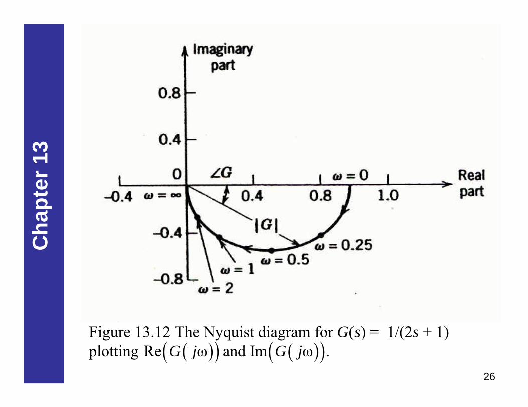
Figure 13.12 The Nyquist diagram for G(s) = 1/(2s + 1) plotting and( )( )Re ωG j ( )( )Im ω .G j

27

Cha

pter

13

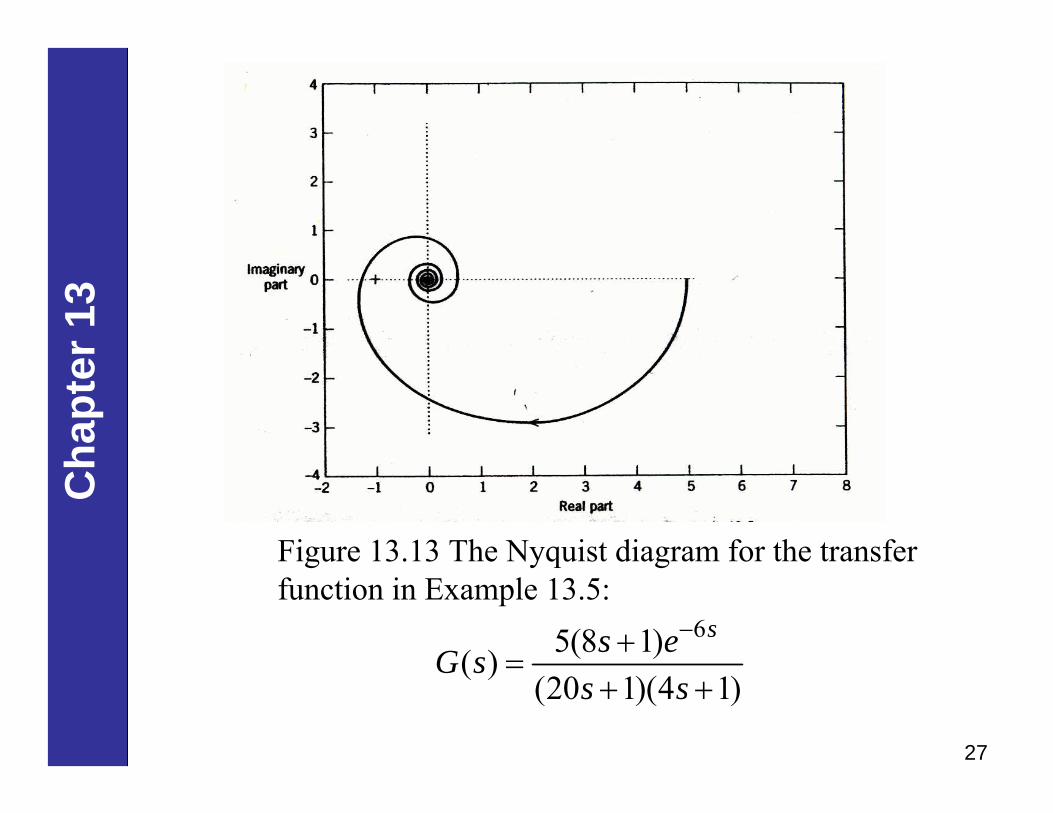
Figure 13.13 The Nyquist diagram for the transfer function in Example 13.5:

65(8 1)( )(20 1)(4 1)

ss eG ss s

−+=

+ +