
Freeform, φ-Polynomial Optical Surfaces: Optical Design ...
202
Freeform, φ-Polynomial Optical Surfaces: Optical Design, Fabrication and Assembly by Kyle Fuerschbach Submitted in Partial Fulfillment of the Requirements for the Degree Doctor of Philosophy Supervised by Professor Jannick Rolland The Institute of Optics Arts, Science and Engineering Edmund A. Hajim School of Engineering and Applied Sciences University of Rochester Rochester, New York 2014
Transcript of Freeform, φ-Polynomial Optical Surfaces: Optical Design ...
Freeform, φ-Polynomial Optical Surfaces:
Optical Design, Fabrication and Assembly
by
Kyle Fuerschbach
Submitted in Partial Fulfillment of the
Requirements for the Degree
Doctor of Philosophy
Supervised by Professor Jannick Rolland
The Institute of Optics
Arts, Science and Engineering
Edmund A. Hajim School of Engineering and Applied Sciences
University of Rochester
Rochester, New York
2014
ii
Biographical Sketch
Kyle Fuerschbach is originally from Albuquerque, NM. After graduating high school, he
attended the University of Arizona in Tucson, AZ and graduated summa cum laude with
a Bachelor of Science degree in Optical Sciences and Engineering. He began doctoral
studies at The Institute of Optics at the University of Rochester in 2008. During his
tenure he was awarded the Robert L. and Mary L. Sproull University Fellowship in 2008,
the Frank J. Horton Research Fellowship from 2008-2014, and the Michael Kidger
Memorial Scholarship in Optical Design in 2011. He has also served as an elected
representative for the University of Rochester’s student chapter of SPIE. He pursued his
research in optical design and fabrication of optical systems with freeform optics under
the direction of Professor Jannick Rolland and co-direction of Dr. Kevin Thompson.
The following peer reviewed publications and patents were a result of work conducted
during doctoral study:
K. Fuerschbach, K. P. Thompson, and J. P. Rolland, "Assembly of an off-axis optical system employing three φ-polynomial, Zernike mirrors," Optics Letters (Accepted to appear April 2014).
K. Fuerschbach, K. P. Thompson, and J. P. Rolland, "Interferometric measurement of a concave, phi-polynomial, Zernike mirror," Optics Letters 39, 18-21 (2014).
J. P. Rolland and K. Fuerschbach, "Nonsymmetric optical system and design method for nonsymmetric optical system," US8616712 B2 (2013).
K. Fuerschbach, J. P. Rolland, and K. P. Thompson, "Extending Nodal Aberration Theory to include mount-induced aberrations with application to freeform surfaces," Opt. Express 20, 20139-20155 (2012).
K. Fuerschbach, J. P. Rolland, and K. P. Thompson, "A new family of optical systems employing phi-polynomial surfaces," Opt. Express 19, 21919-21928 (2011).
S. Vo, K. Fuerschbach, K. P. Thompson, M. A. Alonso, and J. P. Rolland, "Airy beams: a geometric optics perspective," J. Opt. Soc. Am. A 27, 2574-2582 (2010).
iii
Acknowledgments
I would like to thank Professor Jannick Rolland and Dr. Kevin Thompson for their
support and guidance during the Ph.D. process. The original idea to work on a three
mirror freeform design came about when we were deciding what I could present at the
2010 International Optical Design Conference. At the time, I didn’t know it would
eventually become part of my thesis, but through their direction and my hard work, we
were able to explore many avenues in freeform optical surfaces that were all prompted by
the first “pamplemousse” design.
I would like to thank John Miller at the university machine shop and Gregg Davis and
Alan Hedges at II-VI Infrared for providing me with fabrication support. These men
helped translate my crazy ideas into tangible, working pieces of hardware that have been
critical to the success of my research.
I would like to thank all my labmates and officemates: Dr. Cristina Canavesi, Robert
Gray, Jinxin Huang, Jianing Yao, Eric Schiesser, Jacob Reimers, and Aaron Bauer.
Specifically, I would like to thank Aaron Bauer for answering all my questions
throughout the years. He was always willing to help me through a problem or read
something I had written. Thanks also to all the students who helped me with my research
in the lab: Eddie Lavilla, Jean Inard-Charvin, Johan Thivollet, and Isaac Trumper.
Without them, I’d still be in the lab working to get my experiments finished.
Thanks to Elizabeth for her support during my academic career. She made many
personal and professional sacrifices along the way and they have not gone unnoticed.
iv
Also, thanks to my parents, Phil and Marcie, for helping me get to this point. Without
their guidance, I may have never studied optics.
Lastly, I would like to thank my support, the Frank J. Horton Research Fellowship, the
II-VI Foundation, and the National Science Foundation (EECS-1002179) as well as Zygo
for their partnership in optical testing, Synopsys Inc. for the student license of CODE V,
and Photon Engineering for the student license of FRED.
v
Abstract
Freeform optical surfaces are creating exciting new opportunities in optics for design,
fabrication, metrology, and assembly. While the term freeform is currently being applied
over a broad range of surface shapes, in our research on imaging with freeform optical
surfaces, a freeform is a surface whose sag varies not only with the radial component but
also with the azimuthal component, φ, also known as a φ-polynomial optical surface.
Interestingly, these surfaces are readily fabricated with techniques like single point
diamond turning; however, challenges remain in their optimization during optical design
and characterization after fabrication.
In this dissertation, we propose a more effective optical design approach based in
nodal aberration theory that considers the aberrations induced by a φ-polynomial optical
surface up to sixth order. Specifically, when a φ-polynomial overlay is placed on a
surface away from the aperture stop, there is both a field constant and field dependent
contribution to the net aberration field. These findings are validated through the design,
implementation, and wavefront measurement of an aberration generating Schmidt
telescope that employs a custom fabricated φ-polynomial plate. The measured wavefront
behavior is in good agreement with the theoretical predictions of nodal aberration theory
throughout the field of view.
The design methods are also applied to a specific example: a wide field, fast focal
ratio, long wave infrared, unobscured reflective imager. The system employs three, tilted
φ-polynomial surfaces to provide diffraction limited performance throughout the field of
view. The surfaces were fabricated with diamond turning and a novel metrology
vi
approach based on an inteferometric null is proposed for characterizing the figure error of
the fabricated surfaces. A mechanical design is also presented for the housing structure
that simplifies the system assembly. The as-built optical system maintains diffraction
limited performance throughout the field of view.
The work conducted in this dissertation provides a foundation for the efficient design
of optical systems employing freeform surfaces and demonstrates that a system based on
freeform surfaces is realizable in the long wave infrared and may be extended to shorter
wavelength regimes.
vii
Contributors and Funding Sources
This work was supervised by a dissertation committee consisting of Professors Jannick
Rolland (advisor) and Miguel Alonso of The Institute of Optics, Dr. Kevin Thompson of
Synopsys, and Professor Victor Genberg of The Department of Mechanical Engineering.
The original matlab code to plot the Full Field Displays in Chapter 3 and Chapter 4 was
developed by Dr. Christina Dunn. The fabrication of the components and experiments in
Chapter 4 were assisted by Isaac Trumper (undergraduate research assistant) and in part
by Edward Lavilla (summer research assistant). The experiments in Chapter 6 were
assisted in part by Johan Thivollet (graduate research assistant). The mirror surfaces and
optical housing in Chapter 7 were manufactured by II-VI Infrared. All other work
conducted for the dissertation was completed by the student independently. Graduate
study was supported by the Frank J. Horton Research Fellowship from the Laboratory for
Laser Energetics, the II-VI foundation, and the National Science Foundation
(EECS-1002179).
viii
Table of Contents
Biographical Sketch ............................................................................................................ ii
Acknowledgments.............................................................................................................. iii
Abstract ........................................................................................................................... v
Contributors and Funding Sources.................................................................................... vii
Table of Contents ............................................................................................................. viii
List of Figures .................................................................................................................. xiii
List of Tables ................................................................................................................. xxix
List of Acronyms ........................................................................................................... xxxi
Chapter 1. Introduction ....................................................................................................... 1
1.1 Off-Axis Reflective Systems .................................................................................. 1
1.1.1 Offset Aperture and/or Biased Field ................................................................. 2
1.1.2 Tilted Optical Surfaces ..................................................................................... 4
1.2 Freeform Optical Surfaces ...................................................................................... 6
1.3 Motivation ............................................................................................................... 9
1.4 Dissertation Outline .............................................................................................. 14
Chapter 2. Aberration Fields for Tilted and Decentered Optical Systems with
Rotationally Symmetric Components ............................................................. 16
2.1 Aberration Field Centers ....................................................................................... 16
ix
2.2 Wave Aberration Expansion in a Perturbed Optical System ................................ 17
2.3 Full Field Aberration Display ............................................................................... 24
Chapter 3. Aberration Fields in Optical Systems with φ-Polynomial Optical Surfaces ... 29
3.1 Formulating Nodal Aberration Theory for Freeform, ϕ-Polynomial Surfaces away
from the Aperture Stop ......................................................................................... 30
3.2 The Aberration Fields of ϕ-Polynomial Surface Overlays ................................... 36
3.2.1 Zernike Astigmatism ....................................................................................... 37
3.2.2 Zernike Coma .................................................................................................. 41
3.2.3 Zernike Trefoil (Elliptical Coma) ................................................................... 46
3.2.4 Zernike Oblique Spherical Aberration ............................................................ 49
3.2.5 Zernike Fifth Order Aperture Coma ............................................................... 53
3.3 APPLICATION: The Astigmatic Aberration Field Induced by Three Point
Mount-Induced Trefoil Surface Deformation on a Mirror of a Reflective
Telescope .............................................................................................................. 58
3.3.1 Astigmatic Reflective Telescope Configuration ( 222 0W ≠ ) in the Presence of a
Three Point Mount-Induced Surface Deformation on the Secondary Mirror . 60
3.3.2 Anastigmatic Reflective Telescope Configuration ( 222 0W = ) in the Presence of
a Three Point Mount-Induced Surface Deformation on the Secondary Mirror
......................................................................................................................... 64
x
3.3.3 Validation of the Nodal Properties of a Reflective Telescope with Three Point
Mount-Induced Figure Error on the Secondary Mirror .................................. 64
3.4 Extending Nodal Aberration Theory to Include Decentered Freeform
ϕ-Polynomial Surfaces away from the Aperture Stop .......................................... 69
Chapter 4. Experimental Validation of Nodal Aberration Theory for φ-Polynomial
Optical Surfaces .............................................................................................. 72
4.1 Design of an Aberration Generating Schmidt Telescope ..................................... 72
4.2 Fabrication of the Aspheric Corrector/Nonsymmetric Plate ................................ 79
4.3 Experimental Setup of the Aberration Generating Schmidt Telescope ................ 82
4.4 Experimental Results ............................................................................................ 85
4.4.1 The Generated Field Conjugate, Field Linear Astigmatic Field ..................... 85
4.4.2 Rotation of the Aberration Generating Plate .................................................. 89
4.4.3 Lateral Displacement of the Aberration Generating Plate .............................. 90
Chapter 5. Design of a Freeform Unobscured Reflective Imager Employing
φ-Polynomial Optical Surfaces ....................................................................... 93
5.1 The New Method of Optical Design ..................................................................... 93
5.2 The Starting Form ................................................................................................. 95
5.3 The Unobscured Form .......................................................................................... 97
5.3.1 Creating Field Constant Aberration Correction .............................................. 98
xi
5.3.2 Creating Field Dependent Aberration Correction ......................................... 100
5.4 The Final Form ................................................................................................... 104
5.5 Mirror Surface Figures ........................................................................................ 107
Chapter 6. Interferometric Null Configurations for Measuring φ-Polynomial Optical
Surfaces ......................................................................................................... 109
6.1 Concave Surface Metrology ............................................................................... 109
6.1.1 First Order Design......................................................................................... 111
6.1.2 Optimization of the Interferometric Null System ......................................... 117
6.1.3 Experimental Setup of Interferometric Null System .................................... 119
6.1.4 Experimental Results .................................................................................... 124
6.2 Convex Surface Metrology ................................................................................. 127
Chapter 7. Assembly of an Optical System with φ-Polynomial Optical Surfaces ......... 132
7.1 Mechanical Design.............................................................................................. 132
7.1.1 Sensitivity Analysis ...................................................................................... 134
7.1.2 Stray Light Analysis ..................................................................................... 144
7.2 As-built Optical System ...................................................................................... 150
7.2.1 As-built Optical Performance ....................................................................... 152
Conclusion and Future Work .......................................................................................... 158

xii
Appendix A. Vector Multiplication and Its Vector Properties and Identities ............. 163
List of References ........................................................................................................... 166
xiii
List of Figures
Figure 1-1. Demonstration of how an on-axis optical system is made unobscured by
offsetting the aperture, biasing the field, or a combination of both. ....................... 2
Figure 1-2. Single point diamond turning surface roughness evolution through time. Each
color represents a lateral measurement of a part from a specific time period.
(Adapted from Schaefer [45]) ............................................................................... 10
Figure 1-3. Optical design space defined by the light collection (F/number), area
collection (FOV), and packaging for various surface representations. ................. 13
Figure 2-1. Coordinate system for aberration theory of a perturbed optical system where
both the pupil and field coordinate are represented as vectors. ............................ 19
Figure 2-2. Representation of the new effective field vector. ........................................... 20
Figure 2-3. Node locations for third order astigmatism in a perturbed optical system.
There are two points in the field where the aberration can be zero. ..................... 23
Figure 2-4. Full field display (FFD) showing (a) third order field quadratic in a centered
system and (b) in perturbed optical system that yields binodal astigmatism. ....... 28
Figure 3-1. (a) When the aspheric corrector plate of a Schmidt telescope is displaced
longitudinally from the aperture stop, the beam for any off-axis field point will
displace along the corrector plate. The displacement depends on the paraxial
quantities for the marginal ray height, y , chief ray height, y , chief ray angle, u ,
and the distance between the stop and plate, t . (b) Alternatively, the beam
displacement on the corrector plate can be thought of as a field dependent
xiv
decenter of the aspheric corrector, h∆
, that modifies the mapping of the
normalized pupil coordinate from ρ to 'ρ . ........................................................... 33
Figure 3-2. Generation of coma and astigmatism as the aspheric corrector plate in a
Schmidt telescope is moved longitudinally (along the optical axis) from the
physical aperture stop located at the center of curvature of the spherical primary
mirror for various positions (a-d). For each field point in the FFD, the plot symbol
conveys the magnitude and orientation of the aberration. (e) Plots of the
magnitude of coma and astigmatism generated as the aspheric plate is moved
longitudinally for two field points, (0°, 2°) (blue square) and (0°, 4°) (red
triangle). ................................................................................................................ 35
Figure 3-3. Fringe Zernike polynomial set up to 5th order (6th order in wavefront). The set
includes Z1 (piston), Z2/3 (tilt), Z4 (defocus), Z5/6 (astigmatism), Z7/8 (coma), Z9
(spherical aberration), Z10/11 (elliptical coma or trefoil), Z12/13 (oblique spherical
aberration or secondary astigmatism), Z14/15 (fifth order aperture coma or
secondary coma), and Z16 (fifth order spherical aberration or secondary spherical
aberration). The φ-polynomials to be explored include Z5/6, Z7/8, Z10/11, Z12/13, and
Z14/15. ..................................................................................................................... 37
Figure 3-4. Surface map describing the freeform Zernike overlay for astigmatism on an
optical surface over the full aperture. The error is quantified by its magnitude
5/6FFz and its orientation 5/6FFξ that is measured clockwise with respect to the
y − axis. P and V denote where the surface error is a peak rather than a valley. .. 39
xv
Figure 3-5. The characteristic field dependence of field constant astigmatism that is
generated by a Zernike astigmatism overlay on an optical surface in an optical
system. This induced aberration is independent of stop position. ........................ 41
Figure 3-6. The characteristic field dependence of (a) field constant coma, (b) field
asymmetric, field linear astigmatism, and (c) field linear, field curvature that is
generated by a Zernike coma overlay on an optical surface away from the stop
surface. .................................................................................................................. 46
Figure 3-7. The characteristic field dependence of (a) field constant elliptical coma, (b)
field conjugate, field linear astigmatism, which is generated by a Zernike elliptical
coma overlay on an optical surface away from the stop surface. ......................... 49
Figure 3-8. The characteristic field dependence of (a) field constant oblique spherical
aberration, (b) field asymmetric, field linear trefoil, (c) field conjugate, field linear
coma, (d) field constant, field quadratic astigmatism, and (e) field quadratic, field
curvature that is generated by a Zernike oblique spherical aberration overlay on an
optical surface away from the stop surface. .......................................................... 53
Figure 3-9. The characteristic field dependence of (a) field constant, fifth order aperture
coma, (b) field linear medial oblique spherical aberration, (c) field asymmetric,
field linear oblique spherical aberration, (d) field quadratic trefoil, (e) field
quadratic coma, (f) field asymmetric, field cubed astigmatism, and (g) field cubic,
field curvature that is generated by a Zernike fifth order aperture coma overlay on
an optical surface away from the stop surface. ..................................................... 58
xvi
Figure 3-10. (a) The nodal behavior for an optical system with conventional third order
field quadratic astigmatism and Zernike trefoil at a surface away from the stop,
e.g., a two mirror telescope with a three point mount-induced error on the
secondary mirror, is displayed in a reduced field coordinate,Π
, where the node
located by ( )2222 MNTERR x
has an orientation angle of 10/11MNTERRξ and a magnitude that
is proportional to 333,MNTERR SMC
. The two related nodes on the circle are then
advanced by 120º and 240º for this special case. (b) When the nodal solutions are
re-mapped to the conventional field coordinate, H
, the node located by
( )2222 MNTERR x
has an orientation angle of 10/11MNTERRξ and a magnitude that is
proportional to 3333,MNTERR SMC
. ................................................................................. 63
Figure 3-11. A measurement or simulation of the mount-induced error on the secondary
mirror yields the magnitude and orientation of 333,MNTERR SMC
. .................................. 63
Figure 3-12. (a) Layout for a F/8, 300 mm Ritchey-Chrétien telescope and (b) a Full Field
Display (FFD) of the RMS WFE of the optical system at 0.633 µm over a ±0.2°
FOV. Each circle represents the magnitude of the RMS WFE at a particular
location in the FOV. .............................................................................................. 66
Figure 3-13. Displays of the magnitude and orientation of Fringe Zernike astigmatism
(Z5/6) and Fringe Zernike trefoil, elliptical coma, (Z10/11) throughout the FOV for
(a) a Ritchey-Chrétien telescope in its nominal state and (b) the telescope when
0.5λ of three point mount-induced error oriented at 0° has been added to the
xvii
secondary mirror. It is important to recognize that these displays of data are FFDs
that are based on a Zernike polynomial fit to real ray trace OPD data evaluated on
a grid of points in the FOV. For each field point, the plot symbol conveys the
magnitude and orientation of the Zernike coefficients pairs, Z5/6 on the left and
Z10/11 on the right. .................................................................................................. 66
Figure 3-14. (a) Layout for a JWST-like telescope geometry and (b) a Full Field Display
(FFD) of the RMS WFE of the optical system at 1.00 µm over a ±0.2° FOV. The
system utilizes a field bias (outlined in red) to create an accessible focal plane. . 68
Figure 3-15. Displays of the magnitude and orientation of Fringe Zernike astigmatism
(Z5/6) and Fringe Zernike trefoil, elliptical coma, (Z10/11) throughout the FOV for
(a) a JWST-like telescope in its nominal state and (b) the telescope when 0.5λ of
three point mount-induced error oriented at 0° has been added to the secondary
mirror. ................................................................................................................... 68
Figure 3-16. Displays of the magnitude and orientation of Fringe Zernike astigmatism
(Z5/6) and Fringe Zernike trefoil, elliptical coma, (Z10/11) throughout the FOV for a
JWST-like telescope with 0.5λ of three point mount-induced error oriented at 0°
on the off-axis tertiary mirror. .............................................................................. 71
Figure 4-1: Testing configuration for the Schmidt telescope to demonstrate the field
dependent aberration behavior of a freeform optical surface. A freeform, Zernike
plate can purposely be placed at or away from the stop surface to induce field
dependent aberrations. The aberration field behavior of the telescope is measured
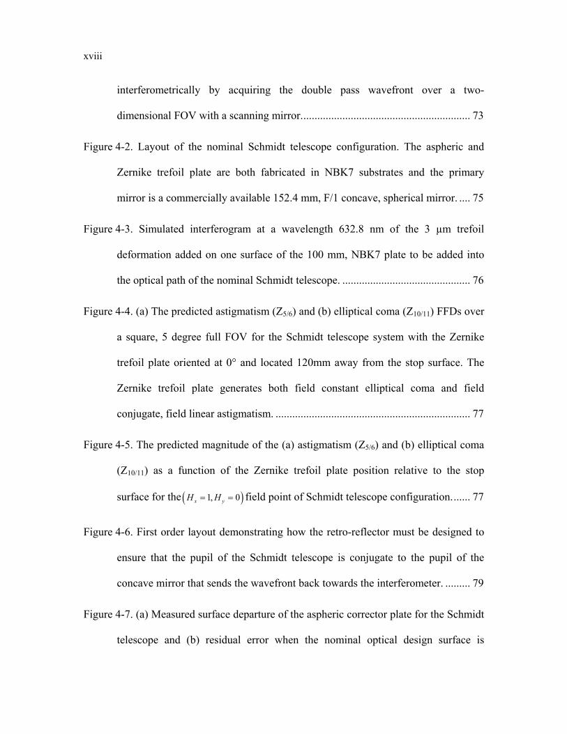
xviii
interferometrically by acquiring the double pass wavefront over a two-
dimensional FOV with a scanning mirror. ............................................................ 73
Figure 4-2. Layout of the nominal Schmidt telescope configuration. The aspheric and
Zernike trefoil plate are both fabricated in NBK7 substrates and the primary
mirror is a commercially available 152.4 mm, F/1 concave, spherical mirror. .... 75
Figure 4-3. Simulated interferogram at a wavelength 632.8 nm of the 3 µm trefoil
deformation added on one surface of the 100 mm, NBK7 plate to be added into
the optical path of the nominal Schmidt telescope. .............................................. 76
Figure 4-4. (a) The predicted astigmatism (Z5/6) and (b) elliptical coma (Z10/11) FFDs over
a square, 5 degree full FOV for the Schmidt telescope system with the Zernike
trefoil plate oriented at 0° and located 120mm away from the stop surface. The
Zernike trefoil plate generates both field constant elliptical coma and field
conjugate, field linear astigmatism. ...................................................................... 77
Figure 4-5. The predicted magnitude of the (a) astigmatism (Z5/6) and (b) elliptical coma
(Z10/11) as a function of the Zernike trefoil plate position relative to the stop
surface for the ( )1, 0x yH H= = field point of Schmidt telescope configuration. ...... 77
Figure 4-6. First order layout demonstrating how the retro-reflector must be designed to
ensure that the pupil of the Schmidt telescope is conjugate to the pupil of the
concave mirror that sends the wavefront back towards the interferometer. ......... 79
Figure 4-7. (a) Measured surface departure of the aspheric corrector plate for the Schmidt
telescope and (b) residual error when the nominal optical design surface is
xix
subtracted from the measured surface. The error is about 0.56λ PV or 0.066λ
RMS at the testing wavelength of 632.8 nm. ........................................................ 81
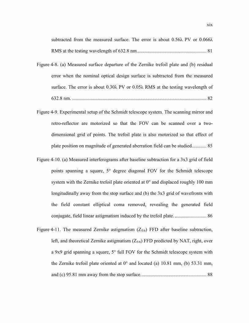
Figure 4-8. (a) Measured surface departure of the Zernike trefoil plate and (b) residual
error when the nominal optical design surface is subtracted from the measured
surface. The error is about 0.30λ PV or 0.05λ RMS at the testing wavelength of
632.8 nm. .............................................................................................................. 82
Figure 4-9. Experimental setup of the Schmidt telescope system. The scanning mirror and
retro-reflector are motorized so that the FOV can be scanned over a two-
dimensional grid of points. The trefoil plate is also motorized so that effect of
plate position on magnitude of generated aberration field can be studied. ........... 85
Figure 4-10. (a) Measured interferograms after baseline subtraction for a 3x3 grid of field
points spanning a square, 5° degree diagonal FOV for the Schmidt telescope
system with the Zernike trefoil plate oriented at 0° and displaced roughly 100 mm
longitudinally away from the stop surface and (b) the 3x3 grid of wavefronts with
the field constant elliptical coma removed, revealing the generated field
conjugate, field linear astigmatism induced by the trefoil plate. .......................... 86
Figure 4-11. The measured Zernike astigmatism (Z5/6) FFD after baseline subtraction,
left, and theoretical Zernike astigmatism (Z5/6) FFD predicted by NAT, right, over
a 9x9 grid spanning a square, 5° full FOV for the Schmidt telescope system with
the Zernike trefoil plate oriented at 0° and located (a) 10.81 mm, (b) 53.31 mm,
and (c) 95.81 mm away from the stop surface. ..................................................... 88
xx
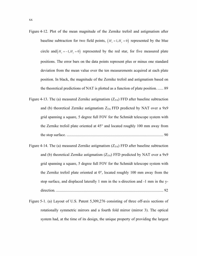
Figure 4-12. Plot of the mean magnitude of the Zernike trefoil and astigmatism after
baseline subtraction for two field points, ( )1, 0x yH H= = represented by the blue
circle and ( )1, 0x yH H= − = represented by the red star, for five measured plate
positions. The error bars on the data points represent plus or minus one standard
deviation from the mean value over the ten measurements acquired at each plate
position. In black, the magnitude of the Zernike trefoil and astigmatism based on
the theoretical predictions of NAT is plotted as a function of plate position. ...... 89
Figure 4-13. The (a) measured Zernike astigmatism (Z5/6) FFD after baseline subtraction
and (b) theoretical Zernike astigmatism Z5/6 FFD predicted by NAT over a 9x9
grid spanning a square, 5 degree full FOV for the Schmidt telescope system with
the Zernike trefoil plate oriented at 45° and located roughly 100 mm away from
the stop surface. .................................................................................................... 90
Figure 4-14. The (a) measured Zernike astigmatism (Z5/6) FFD after baseline subtraction
and (b) theoretical Zernike astigmatism (Z5/6) FFD predicted by NAT over a 9x9
grid spanning a square, 5 degree full FOV for the Schmidt telescope system with
the Zernike trefoil plate oriented at 0°, located roughly 100 mm away from the
stop surface, and displaced laterally 1 mm in the x-direction and -1 mm in the y-
direction. ............................................................................................................... 92
Figure 5-1. (a) Layout of U.S. Patent 5,309,276 consisting of three off-axis sections of
rotationally symmetric mirrors and a fourth fold mirror (mirror 3). The optical
system had, at the time of its design, the unique property of providing the largest
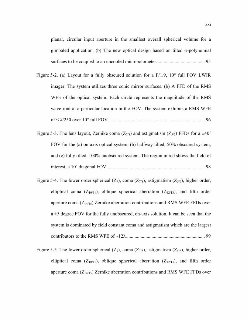
xxi
planar, circular input aperture in the smallest overall spherical volume for a
gimbaled application. (b) The new optical design based on tilted φ-polynomial
surfaces to be coupled to an uncooled microbolometer. ....................................... 95
Figure 5-2. (a) Layout for a fully obscured solution for a F/1.9, 10° full FOV LWIR
imager. The system utilizes three conic mirror surfaces. (b) A FFD of the RMS
WFE of the optical system. Each circle represents the magnitude of the RMS
wavefront at a particular location in the FOV. The system exhibits a RMS WFE
of < λ/250 over 10° full FOV. ............................................................................... 96
Figure 5-3. The lens layout, Zernike coma (Z7/8) and astigmatism (Z5/6) FFDs for a ±40˚
FOV for the (a) on-axis optical system, (b) halfway tilted, 50% obscured system,
and (c) fully tilted, 100% unobscured system. The region in red shows the field of
interest, a 10˚ diagonal FOV. ................................................................................ 98
Figure 5-4. The lower order spherical (Z9), coma (Z7/8), astigmatism (Z5/6), higher order,
elliptical coma (Z10/11), oblique spherical aberration (Z12/13), and fifth order
aperture coma (Z14/15) Zernike aberration contributions and RMS WFE FFDs over
a ±5 degree FOV for the fully unobscured, on-axis solution. It can be seen that the
system is dominated by field constant coma and astigmatism which are the largest
contributors to the RMS WFE of ~12λ. ................................................................ 99
Figure 5-5. The lower order spherical (Z9), coma (Z7/8), astigmatism (Z5/6), higher order,
elliptical coma (Z10/11), oblique spherical aberration (Z12/13), and fifth order
aperture coma (Z14/15) Zernike aberration contributions and RMS WFE FFDs over

xxii
a ±5 degree FOV for the optimized system where Zernike astigmatism and coma
were used as variables on the secondary (stop) surface. When the system is
optimized, the field constant contribution to astigmatism and coma are greatly
reduced improving the RMS WFE from ~12λ to ~0.75λ. .................................. 100
Figure 5-6. The lower order spherical (Z9), coma (Z7/8), astigmatism (Z5/6), higher order,
elliptical coma (Z10/11), oblique spherical aberration (Z12/13), and fifth order
aperture coma (Z14/15) Zernike aberration and RMS WFE FFDs over a ±5 degree
FOV for the optimized system where Zernike coma is added as an additional
variable to the primary surface. The RMS WFE has been reduced from ~0.75λ to
~0.125λ. .............................................................................................................. 102
Figure 5-7. The lower order spherical (Z9), coma (Z7/8), astigmatism (Z5/6), higher order,
elliptical coma (Z10/11), oblique spherical aberration (Z12/13), and fifth order
aperture coma (Z14/15) Zernike aberration contributions and RMS WFE FFDs over
a ±5 degree FOV for the optimized system where Zernike coma is added as an
additional variable to the tertiary surface. The RMS WFE has been reduced from
~0.75λ to ~0.180λ. .............................................................................................. 103
Figure 5-8. The lower order spherical (Z9), coma (Z7/8), astigmatism (Z5/6), higher order,
elliptical coma (Z10/11), oblique spherical aberration (Z12/13), and fifth order
aperture coma (Z14/15) Zernike aberration contributions and RMS WFE FFDs over
a ±5 degree FOV for the optimized system where the mirror conic constants are
added as additional variables in addition to Zernike elliptical coma, oblique
xxiii
spherical aberration, fifth order aperture coma on the secondary surface. The
RMS WFE has been reduced from ~0.180λ to ~0.065λ. .................................... 105
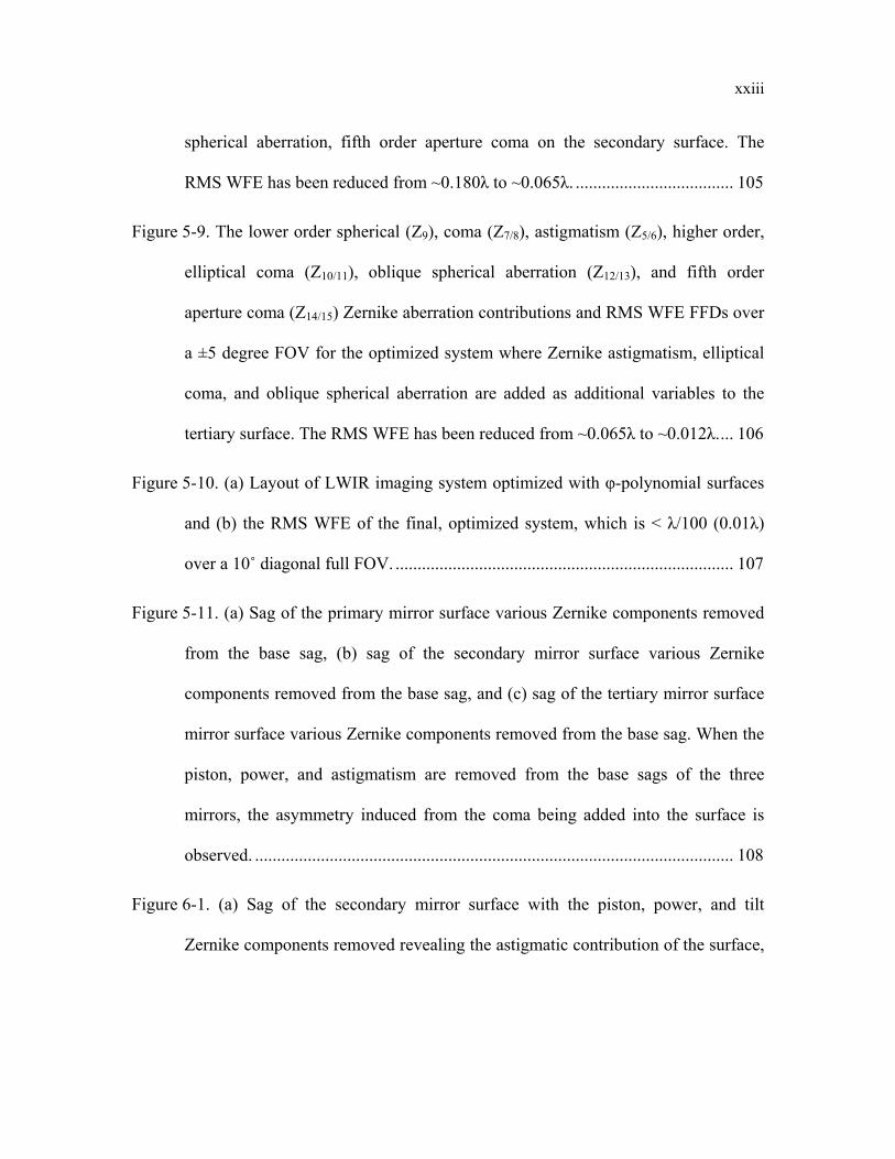
Figure 5-9. The lower order spherical (Z9), coma (Z7/8), astigmatism (Z5/6), higher order,
elliptical coma (Z10/11), oblique spherical aberration (Z12/13), and fifth order
aperture coma (Z14/15) Zernike aberration contributions and RMS WFE FFDs over
a ±5 degree FOV for the optimized system where Zernike astigmatism, elliptical
coma, and oblique spherical aberration are added as additional variables to the
tertiary surface. The RMS WFE has been reduced from ~0.065λ to ~0.012λ. ... 106
Figure 5-10. (a) Layout of LWIR imaging system optimized with φ-polynomial surfaces
and (b) the RMS WFE of the final, optimized system, which is < λ/100 (0.01λ)
over a 10˚ diagonal full FOV. ............................................................................. 107
Figure 5-11. (a) Sag of the primary mirror surface various Zernike components removed
from the base sag, (b) sag of the secondary mirror surface various Zernike
components removed from the base sag, and (c) sag of the tertiary mirror surface
mirror surface various Zernike components removed from the base sag. When the
piston, power, and astigmatism are removed from the base sags of the three
mirrors, the asymmetry induced from the coma being added into the surface is
observed. ............................................................................................................. 108
Figure 6-1. (a) Sag of the secondary mirror surface with the piston, power, and tilt
Zernike components removed revealing the astigmatic contribution of the surface,
xxiv
(b) sag with the astigmatic component additionally removed, and (c) sag with the
spherical component additionally removed. ....................................................... 110
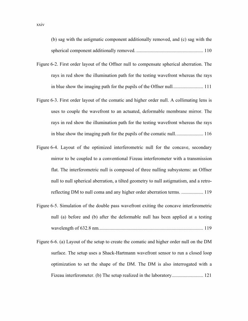
Figure 6-2. First order layout of the Offner null to compensate spherical aberration. The
rays in red show the illumination path for the testing wavefront whereas the rays
in blue show the imaging path for the pupils of the Offner null. ........................ 111
Figure 6-3. First order layout of the comatic and higher order null. A collimating lens is
uses to couple the wavefront to an actuated, deformable membrane mirror. The
rays in red show the illumination path for the testing wavefront whereas the rays
in blue show the imaging path for the pupils of the comatic null. ...................... 116
Figure 6-4. Layout of the optimized interferometric null for the concave, secondary
mirror to be coupled to a conventional Fizeau interferometer with a transmission
flat. The interferometric null is composed of three nulling subsystems: an Offner
null to null spherical aberration, a tilted geometry to null astigmatism, and a retro-
reflecting DM to null coma and any higher order aberration terms. .................. 119
Figure 6-5. Simulation of the double pass wavefront exiting the concave interferometric
null (a) before and (b) after the deformable null has been applied at a testing
wavelength of 632.8 nm. ..................................................................................... 119
Figure 6-6. (a) Layout of the setup to create the comatic and higher order null on the DM
surface. The setup uses a Shack-Hartmann wavefront sensor to run a closed loop
optimization to set the shape of the DM. The DM is also interrogated with a
Fizeau interferometer. (b) The setup realized in the laboratory. ......................... 121
xxv
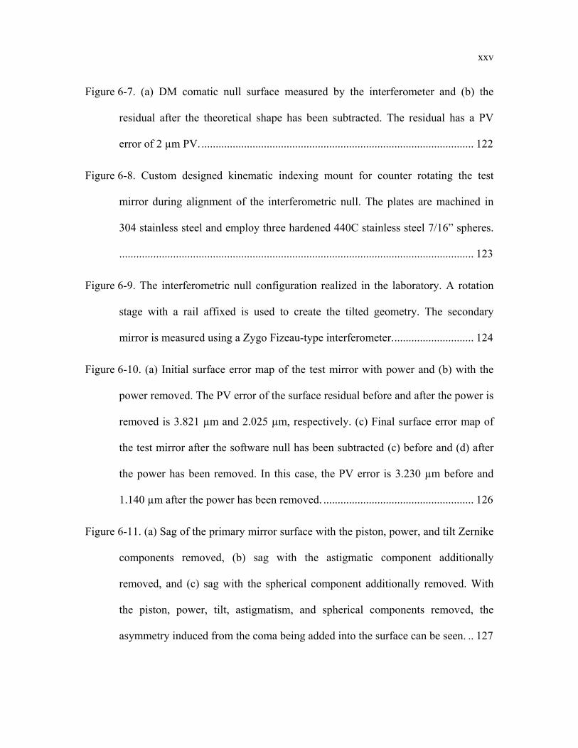
Figure 6-7. (a) DM comatic null surface measured by the interferometer and (b) the
residual after the theoretical shape has been subtracted. The residual has a PV
error of 2 µm PV. ................................................................................................ 122
Figure 6-8. Custom designed kinematic indexing mount for counter rotating the test
mirror during alignment of the interferometric null. The plates are machined in
304 stainless steel and employ three hardened 440C stainless steel 7/16” spheres.
............................................................................................................................. 123
Figure 6-9. The interferometric null configuration realized in the laboratory. A rotation
stage with a rail affixed is used to create the tilted geometry. The secondary
mirror is measured using a Zygo Fizeau-type interferometer. ............................ 124
Figure 6-10. (a) Initial surface error map of the test mirror with power and (b) with the
power removed. The PV error of the surface residual before and after the power is
removed is 3.821 µm and 2.025 µm, respectively. (c) Final surface error map of
the test mirror after the software null has been subtracted (c) before and (d) after
the power has been removed. In this case, the PV error is 3.230 µm before and
1.140 µm after the power has been removed. ..................................................... 126
Figure 6-11. (a) Sag of the primary mirror surface with the piston, power, and tilt Zernike
components removed, (b) sag with the astigmatic component additionally
removed, and (c) sag with the spherical component additionally removed. With
the piston, power, tilt, astigmatism, and spherical components removed, the
asymmetry induced from the coma being added into the surface can be seen. .. 127
xxvi
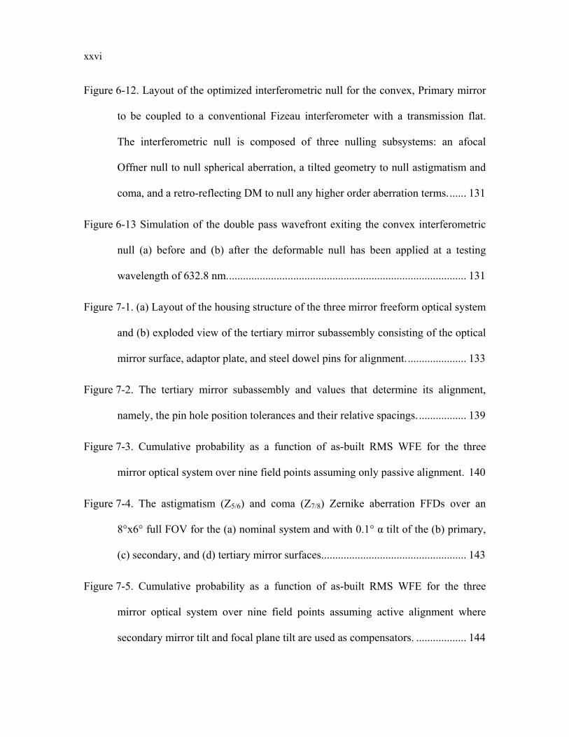
Figure 6-12. Layout of the optimized interferometric null for the convex, Primary mirror
to be coupled to a conventional Fizeau interferometer with a transmission flat.
The interferometric null is composed of three nulling subsystems: an afocal
Offner null to null spherical aberration, a tilted geometry to null astigmatism and
coma, and a retro-reflecting DM to null any higher order aberration terms. ...... 131
Figure 6-13 Simulation of the double pass wavefront exiting the convex interferometric
null (a) before and (b) after the deformable null has been applied at a testing
wavelength of 632.8 nm. ..................................................................................... 131
Figure 7-1. (a) Layout of the housing structure of the three mirror freeform optical system
and (b) exploded view of the tertiary mirror subassembly consisting of the optical
mirror surface, adaptor plate, and steel dowel pins for alignment. ..................... 133
Figure 7-2. The tertiary mirror subassembly and values that determine its alignment,
namely, the pin hole position tolerances and their relative spacings. ................. 139
Figure 7-3. Cumulative probability as a function of as-built RMS WFE for the three
mirror optical system over nine field points assuming only passive alignment. 140
Figure 7-4. The astigmatism (Z5/6) and coma (Z7/8) Zernike aberration FFDs over an
8°x6° full FOV for the (a) nominal system and with 0.1° α tilt of the (b) primary,
(c) secondary, and (d) tertiary mirror surfaces. ................................................... 143
Figure 7-5. Cumulative probability as a function of as-built RMS WFE for the three
mirror optical system over nine field points assuming active alignment where
secondary mirror tilt and focal plane tilt are used as compensators. .................. 144
xxvii
Figure 7-6. The computed elevation log(PST) for the baseline optical housing with the
walls of the housing material assumed to be machined aluminum, resulting in a
near specular surface with 80% reflectance. ....................................................... 146
Figure 7-7. The computed elevation log(PST) for the optical system with blackened walls
in blue and the computed elevation log(PST) for the baseline optical housing in
gray. An improvement is observed when the walls of the housing are blackened
versus left machined aluminum. ......................................................................... 147
Figure 7-8. Cutaway of the optical system (a) without a baffle and (b) with a baffle and
its solid angle to the environment from the focal plane shown in red for each case.
With the baffle added to the housing, the solid angle to the environment goes to
zero. ..................................................................................................................... 148
Figure 7-9. The computed elevation log(PST) for the optical system with blackened walls
as well as baffling near the image plane in red and the computed elevation
log(PST) for the optical housing with blackened walls in light blue. A two order
of magnitude improvement is observed in the regions of large stray light when
baffling is added near the image plane. .............................................................. 149
Figure 7-10. The computed elevation log(PST) for the optical system with blackened
walls, baffling near the image plane, and baffling at the primary mirror in green
and the computed elevation log(PST) for the optical housing with blackened walls
and baffling near the image plane in light red. A two order of magnitude
xxviii
improvement is observed for large positive elevation angles where scattering is
the dominant contributor to stray light. ............................................................... 150
Figure 7-11. As-built subassemblies for the (a) primary, (b) secondary, and (c) tertiary
mirrors of the three mirror system that are to be mated to the optical housing.
Each subassembly mates to one face of the optical housing and rests on three
raised, diamond turned pads. .............................................................................. 151
Figure 7-12. Assembled three mirror optical system. The system consists of a housing
structure and three mirror subassemblies that are mated to the faces of the
housing. ............................................................................................................... 151
Figure 7-13. Experimental setup for measuring the full field performance of the as-built
optical system...................................................................................................... 153
Figure 7-14. Measured wavefronts for a 3x3 grid of field points spanning an
8 mm x 6 mm FOV for the directly assembled three mirror optical system. The
RMS WFE in microns displayed within the wavefront for each field. ............... 155
Figure 7-15. Measured wavefronts for a 3x3 grid of field points spanning an
8 mm x 6 mm FOV for the directly assembled three mirror optical system with
the secondary mirror tilted roughly 1 arc minute with a 23 µm shim. The RMS
WFE in microns is displayed within the wavefront for each field. .................... 157
Figure 7-16. Sample LWIR image from the optical system ........................................... 157
Figure A-1. Concept of vector multiplication. ................................................................ 164
xxix
List of Tables
Table 2-1. Names of the aberration terms from the wavefront expansion up to fifth order.
............................................................................................................................... 18
Table 2-2. Summary of the first sixteen Fringe Zernike polynomials and their relation to
the standard Zernike set. ....................................................................................... 26
Table 2-3. Field dependence of the Zernike coefficients in terms of the wave aberration
coefficients. (Adapted from Gray et al. [35]) ....................................................... 27
Table 3-1. Field aberration terms that are generated from the longitudinal shift of an
aspheric plate from the stop surface in a Schmidt telescope. ............................... 33
Table 3-2. Image degrading aberration terms that are generated by a Zernike coma
overlay and how the terms link to existing concepts of NAT ............................... 45
Table 3-3. Image degrading aberration terms that are generated by a Zernike elliptical
coma overlay and how the terms link to existing concepts of NAT ..................... 47
Table 3-4. Image degrading aberration terms that are generated by a Zernike oblique
spherical aberration overlay and how the terms link to existing concepts of NAT
............................................................................................................................... 52
Table 3-5. Image degrading aberration terms that are generated by a Zernike fifth order
aperture coma overlay and how the terms link to existing concepts of NAT ....... 56
Table 4-1. Design specifications for the nominal aberration generating Schmidt telescope.
............................................................................................................................... 75

xxx
Table 7-1. Summary of the initial sensitivity analysis of the three mirror optical system.
For each tolerance, the change in RMS WFE from nominal is computed and the
RSS is compiled to provide the as-built RMS WFE. The RMS WFE is terms of
waves at the central operating wavelength of 10 µm. ......................................... 136
Table 7-2. Summary of the quantities used to derive the tolerances for the Monte Carlo
sensitivity analysis. The pin hole tolerances are used to derive the mirror x/y
decenter and mirror clocking angle. .................................................................... 139
xxxi
List of Acronyms
CGH Computer Generated Hologram
COTS Commercial Off The Shelf
DM Deformable Mirror
DOF(s) Degree(s) of Freedom
FFD Full Field Display
FOV(s) Field(s) of View
JWST James Webb Space Telescope
LWIR Long Wave InfraRed
MRF MagnetoRheological Finishing
NAT Nodal Aberration Theory
OAR Optical Axis Ray
OPD Optical Path Difference
PST Point Source Transmittance
PV Peak to Valley
RMS Root Mean Square
RSS Root Sum Square
TMA Three Mirror Anastigmat
WALRUS Wide Angle Large Reflective System
WFE Wavefront Error

1
Chapter 1. Introduction
In the introductory part of this dissertation, a brief history of off-axis reflective systems
and freeform optical surfaces is presented. Our motivation for this research is then
presented and the dissertation is outlined.
1.1 Off-Axis Reflective Systems
Reflective telescopes are commonly used for astronomical and earth based surveying
because they provide large apertures for light collection; however, most classical
telescope forms, i.e. Newtonian, Cassegrain, Gregorian, and Ritchey-Chrétien, have an
obscured aperture that will affect the overall image quality from diffraction of the
obscuration and its spider supports. The obscuration may also cause stray light in infrared
applications because the warm mechanical structure from the obscuration exists in the
beam path. Handling the obscuring aperture and creating an accessible image plane
becomes even more difficult when trying to design a system to correct the three primary
aberrations, i.e. spherical aberration, coma, and astigmatism, where three mirror surfaces
are required [1-3].
One way to avoid an obscured configuration is to operate off-axis creating an
unobscured form. Historically, there are two principal ways to operate off-axis. The first
is to take a nominally rotationally symmetric reflective form and either offset the
aperture, bias the field, or a combination of both [4]. In this configuration each optical
surface is a section of a larger parent surface where each parent surface lies on a common
optical axis. The other way to operate off-axis is to tilt the optical surfaces themselves to
create an unobscured form [5, 6]. In this fashion, each optical surface is not arranged
along a common optical axis. In some unobscured configurations that tilt the optical
2
surfaces, a nonsymmetric surface is employed to restore the optical performance after the
surfaces have been tilted [6].
1.1.1 Offset Aperture and/or Biased Field
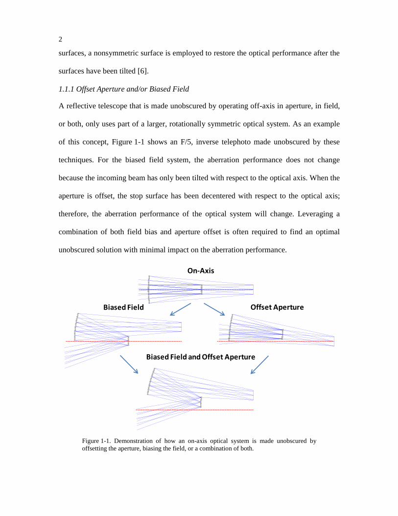
A reflective telescope that is made unobscured by operating off-axis in aperture, in field,
or both, only uses part of a larger, rotationally symmetric optical system. As an example
of this concept, Figure 1-1 shows an F/5, inverse telephoto made unobscured by these
techniques. For the biased field system, the aberration performance does not change
because the incoming beam has only been tilted with respect to the optical axis. When the
aperture is offset, the stop surface has been decentered with respect to the optical axis;
therefore, the aberration performance of the optical system will change. Leveraging a
combination of both field bias and aperture offset is often required to find an optimal
unobscured solution with minimal impact on the aberration performance.
10:01:52
New lens from CVMACRO:cvnewlens.seq Scale: 0.64 13-Mar-14
39.06 MM
09:57:43
New lens from CVMACRO:cvnewlens.seq Scale: 0.65 13-Mar-14
38.46 MM
09:56:30
New lens from CVMACRO:cvnewlens.seq Scale: 0.64 13-Mar-14
39.06 MM
10:02:21
New lens from CVMACRO:cvnewlens.seq Scale: 0.65 13-Mar-14
38.46 MM
On-Axis
Biased Field Offset Aperture
Biased Field and Offset Aperture
Figure 1-1. Demonstration of how an on-axis optical system is made unobscured by
offsetting the aperture, biasing the field, or a combination of both.
3
One of the earliest three mirror forms that used aperture offset and field bias was
introduced by Cook [7, 8] who took a three mirror anastigmat (TMA) form by Korsch [9]
off-axis in aperture and field. Each mirror is an off-axis conic section with the primary
and secondary elements forming a Cassegrainian pair that creates an intermediate image.
The image is then re-imaged with a tertiary element of approximately unit magnification.
The design has the degrees of freedom (DOFs) to provide an aplanatic, anastigmatic, and
flat image plane. This type of system is useful for infrared applications because it has an
accessible exit pupil, but is best suited for a narrow, strip field of view (FOV).
Another set of unobscured forms with large FOVs were created in the late 1970s by
using combinations of systems that are designed with symmetry principles in mind.
These principles are: stop at the center of curvature of a sphere (i.e. Schmidt telescope),
concentricity about the object/image or pupil (i.e. Schwarzschild objective), and confocal
(Mersenne) parabolas [10]. From these principles, several wide field obscured forms can
be derived from which an unobscured form is obtained. The basic form found by Baker
[11] combines confocal parabolas with a Schmidt telescope to form an aplanatic,
anastigmatic telescope objective. In this configuration, the secondary element, which is
located at the center of curvature of the tertiary, is aspherized to provide spherical
aberration correction. Two other variations of the form presented by Baker are the
reflective triplet [12], which is on-axis in aperture but off-axis in field, and the wide angle
large reflective system (WALRUS) [13], which is an inverse Baker design. These designs
yield larger FOVs than the TMA and maintain similar performance but sacrifice the
accessible exit pupil.
4
A still larger FOV is achieved in a three mirror unobscured form by using a principle
proposed by Brueggemann in which the stop surface is placed at one of the mathematical
foci of a conic mirror to remove astigmatism [14]. Following this principle Egdall formed
a three mirror objective called the three mirror long using a hyperboloidal primary and an
ellipsoidal tertiary [15]. A nearly flat secondary is placed at the common conic focus and
serves as the stop of the optical system to correct astigmatism. By aspherizing this
element, spherical aberration can also be corrected creating an aplanatic, anastigmatic
objective. The shortcomings of this configuration are its length, usually around four focal
lengths [16], and its mirrors, which will have a larger diameter than the entrance pupil of
the system when using a large FOV.
1.1.2 Tilted Optical Surfaces
Another approach to create an unobscured system is to tilt the optical surfaces directly.
For this method there are several approaches on how to create an unobscured optical
system from tilted components. One approach takes a well corrected system that is
nominally rotationally symmetric and adjusts the tilts of the optical surfaces to create an
unobscured form [6]. The performance of the optical system after applying the tilt is
restored by adjusting the system parameters or by adding additional DOFs to the optical
surfaces by changing their surface shape.
One of the first examples of a system designed with this method was introduced by
Kutter where he took a two mirror telescope and tilted the mirrors in a configuration that
removes the obscuration while keeping the astigmatism and coma at a minimum [17].
Leonard used similar principles to obtain a three mirror telescope he called the Yolo that
used two conic elements and one anamorphic conic (different curvatures in orthogonal
5
directions) [18]. The system is slow at roughly F/12 but provides good performance over
a 2° diameter field. Buchroeder [5] developed a modified Seidel aberration theory to
understand the behavior of tilted component systems. In his theory the net aberration
fields are still the superposition of the individual surface aberration field contributions;
however, each contribution will have its own center defined by its decentration or tilt.
Shack [19] then developed an expression for the wave aberration expansion that used the
concepts of Buchroeder. In the new expansion of the wave aberration, the aberration
types can have multiple points in the field where they may go to zero and these zeros are
called nodes. The theory of Shack, often called vector or nodal aberration theory (NAT),
was developed through fifth order by Thompson [20-25] and was applied to the
tolerancing of optical systems. Rogers applied NAT as a design technique for three
mirror telescope objectives [26-28]. In his method, two tilted optical components are
combined to yield a system with linear coma and constant astigmatism. Next, a third
optical element is added with some cylindrical power to eliminate axial astigmatism.
Lastly, the elements are aspherized to correct the residual coma and spherical aberration.
With this method systems of similar performance to the Yolo are obtained in a different
packaging geometry. The Yolo and the systems proposed by Rogers are slow (greater
than F/10), have small FOVs, and do not utilize freeform surfaces to improve
performance; rather, they are special configurations where the net aberration fields are
arranged to be near zero.
In another approach, the optical system is designed from the outset in an unobscured
form. Systems designed in this manner require a method to set up the initial system
parameters but give the designer the freedom to control the geometry, i.e. volume, while
6
selecting an initial design. One method to generate systems composed of three spherical
mirrors has been proposed by Howard [29]. In this method, the imaging properties about
a central ray are Taylor expanded. The coefficients of this expansion represent the first
order imaging properties and are used to constrain the system parameters like the
distances between elements, curvatures of the mirrors, and their tilts. Only solutions that
yield no first order blur are considered and these solutions are found using a systematic
search or a global optimization technique. Such a method allows the designer to explore a
larger design space more rapidly but does not guarantee a practical solution with useful
performance. Another three mirror, tilted component system has been proposed by
Nakano [30] in which the geometry is derived to maximize the compactness as well as
the input aperture. Setting the optical path configuration fixes the mirror positions and
then Cartesian surfaces are used to correct spherical aberration and minimize
astigmatism. Coma is minimized by adding higher than second order deformation to the
surfaces. The system achieves a compact geometry operating over a 4°x4° square FOV at
F/2.2.
1.2 Freeform Optical Surfaces
In the systems described above, the symmetry of the optical system is broken out of
necessity, either to avoid an obscuration or to meet the size and/or weight constraints of
the optical system. However, in general, unless special configurations are exploited, the
performance of the optical system degrades when the system symmetry is broken. As a
result, the surfaces of the optical system can be freeform to help recover from the
performance degradation. We define freeform surfaces as nonsymmetric surfaces that
include coma and potentially higher orders to their surface departure and go beyond
7
anamorphic. One of the first examples of an optical system that utilized a freeform
optical surface is the Polaroid SX-70 [31]. The commercial product was designed to be
collapsible and the need for flatness of the overall package prompted Baker, the lead
optical designer, to use mirrors rather than a penta-prism for the viewfinder. The
constraints on the system geometry forced the use of two freeform lenses that are
described by up to an eighth order power series in both the x and y directions of the
optical surface.
Around the same time, Tatian [32-34] began studying nonsymmetric surfaces for the
design of unobscured reflective systems. The surface representation dubbed the “unusual
optical surface” is described by a section of an aspheric surface with bilateral symmetry
in both the x and y directions where within the local origin of the section may exist up to
a tenth order power series in both the x and y directions. With this surface description,
Tatian was able to achieve roughly a 3X improvement in the root mean square (RMS)
wavefront error (WFE) of a three mirror WALRUS design with unusual surfaces versus
the same design with only aspheric surfaces.
Shafer also applied a nonsymmetric optical surface to the design of unobscured
systems. In his approach, he proposed a two-axis aspheric surface that is the summation
of two aspheres that are shifted relative to one another and may be anamorphically
stretched. In the region that these two aspheres overlap, lower order aberration
contributions like coma and astigmatism are generated. With this approach, special
optical configurations like a two-axis asphere at a pupil location can be exploited to yield
an unobscured two mirror optical system that is corrected for all third order aberrations.
Shafer mentions that these surfaces could be described and optimized with a
8
two-dimensional polynomial set over the entire surface, but the computational power
required to do so at the time was prohibitive. More recently, now that computational
power is no longer nearly as restrictive, two-dimensional polynomial sets to describe an
optical surface have started to appear. As mentioned in Section 1.1.2, Nakano [30] used
an orthogonal polynomial set called the Zernike polynomial set (described in detail in
Chapter 2) to describe an optical surface. The Zernike set is expressed in polar
coordinates and is desirable as it directly relates to the wavefront aberrations proposed by
Hopkins [35]. A related two-dimensional orthogonal polynomial set has been proposed
by Forbes [36] to describe freeform surfaces. Forbes’ set is also based on Jacobi
polynomials but arranged and normalized so that the slope of the optical surface can be
minimized. Also, rigid body terms like defocus and tilt have been eliminated from the
description. Since both the set proposed by Forbes and the Zernike polynomial set are
orthogonal, they can be used interchangeably to describe one another.
The surface representations described above consider the global surface shape so that
the variables describing the surface affect the entire surface. A more localized optical
representation based on a bicubic spline has been proposed for nonsymmetric optical
systems by Vogl et al. [37] and implemented further by Stacy [38] for the design of an
unobscured optical system. For a spline surface, the optical surface is sampled by a grid
of points. At each point, the surface deformation at that point becomes a variable that can
be optimized. The values between these mesh points are interpolated by a cubic
polynomial. A benefit of the spline surface is that the deformations at each point are only
partially correlated to surrounding points. Stacy applied the spline surface to a mirror
near the focal plane of a four mirror telescope to improve the field performance of the
9
system. The final surface shape exhibited strong oscillations that do cause image
degradation. Spline surfaces are computationally intensive because many variables are
required to describe them. Another approach at local shape control was proposed by
Cakmakci et al. [39] where the optical surface is written as a sum of basis functions, in
this case, a two-dimensional Gaussian. In this approach, the surface is sampled by a grid
of points where at each point, the Gaussian shape can be varied. This surface description
was applied to a single mirror head-worn display. In a local approach the key is to ensure
that the performance metric of the optical system is appropriately sampled throughout the
FOV [40, 41]. For this reason, a global or hybrid surface representation may be more
effective for a sparsely sampled field that is often the case during optimization in optical
design.
1.3 Motivation
The concept of a freeform optical surface is not new and was recognized early on as a
promising tool for the design of the nonsymmetric optical systems; however, unless the
surfaces can be manufactured, they are little more than an academic exercise. For
example, in 1972, Gelles when studying unobscured two mirror systems wrote that
“progress in surface generation will undoubtedly permit the use of exotic types of
surfaces in the future” [42]. Until recently, the fabrication capabilities did not exist to
manufacture these types of optical surfaces in a cost effective manner. One of these
recent advances has been in diamond turning technology where servos have been
integrated into the axes geometry in either a fast tool servo or slow slide servo
configuration [43, 44]. This integration allows for surfaces that are nonsymmetric to be
routinely manufactured. Moreover, the residual surface roughness after diamond turning
10
has been reduced so that post-polishing is no longer required, further reducing the cost of
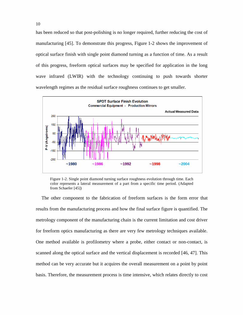
manufacturing [45]. To demonstrate this progress, Figure 1-2 shows the improvement of
optical surface finish with single point diamond turning as a function of time. As a result
of this progress, freeform optical surfaces may be specified for application in the long
wave infrared (LWIR) with the technology continuing to push towards shorter
wavelength regimes as the residual surface roughness continues to get smaller.
Actual Measured Data
~1980 ~1986 ~1992 ~1998 ~2004
Figure 1-2. Single point diamond turning surface roughness evolution through time. Each
color represents a lateral measurement of a part from a specific time period. (Adapted
from Schaefer [45])
The other component to the fabrication of freeform surfaces is the form error that
results from the manufacturing process and how the final surface figure is quantified. The
metrology component of the manufacturing chain is the current limitation and cost driver
for freeform optics manufacturing as there are very few metrology techniques available.
One method available is profilometry where a probe, either contact or non-contact, is
scanned along the optical surface and the vertical displacement is recorded [46, 47]. This
method can be very accurate but it acquires the overall measurement on a point by point
basis. Therefore, the measurement process is time intensive, which relates directly to cost
11
on the manufacturing floor. Another method is based on the use of a computer generated
hologram (CGH) that acts as a nulling component in an interferometric arrangement [48].
The quality of the measurement obtained with the CGH depends strongly on the
fabrication of the CGH and the arrangement in which it is placed in the
interferometer [49]. Moreover, each CGH is unique to one specific surface and can be
cost prohibitive for multiple surfaces [50]. Another potential method is to arrange optical
elements (i.e. lenses or mirrors) in a null configuration. These methods exist for
measuring off-axis sections of conics and aspherics [51] but have not been developed for
freeform surfaces.
In addition to fabrication, one of the challenges with freeform optical surfaces is the
excess of variables introduced during optimization. If a global surface representation like
the Zernike polynomial set is used, the optical designer has access to an impractical
number of variables per surface during optimization. In a more localized approach, the
number of coefficients grows rapidly as the sampling is increased on the optical surface.
In 1978, Shafer recognized this point and to motivate his two-axis asphere approach over
a set of polynomials, he wrote, “…a Zernike set of aspheric coefficients would be able to
describe these surfaces and could be used to design systems. That, however, would be a
very cumbersome way to proceed, and would probably have a poor convergence rate
during optimization” [52]. Even with modern day computational power, where the time
per optimization cycle is minimal, a more efficient approach for choosing which surfaces
would benefit from a freeform surface and which variables to optimize on the surface is
desirable.
12
With the challenges described above for the design and fabrication of a freeform
surface, there has to be some direct benefit that cannot be achieved without a freeform
surface to justify their use in an optical system. To describe this benefit, consider the
specifications of an optical system. Any optical system will be required to meet some sort
of image quality metric with a certain light collection capability like F/number and with a
certain area coverage like FOV. Another more esoteric constraint may be the packaging
of the optical system. For example, the weight or size of the optical system might be
constrained for certain applications. These three items, F/number, FOV, and packaging,
define the design space for optical design. The extent of the design space that may be
covered by a particular surface representation is demonstrated in Figure 1-3. The most
restrictive optical design shape is the sphere. If the package is to be made smaller with
the same performance, thus widening the optical design space, conics or aspheric surfaces
are usually employed. Examples here are the use of conics in astronomical applications
[14, 53] and the use of aspheres for mobile phone optics [54]. If non-inline geometries
are considered like a tilted or decentered optical system, the aberration correction
capability is limited with conic or aspheric surfaces. Innovative packaging geometries are
the strength of freeform surfaces as they provide the necessary DOFs to operate in this
space, thus, increasing the optical design space.
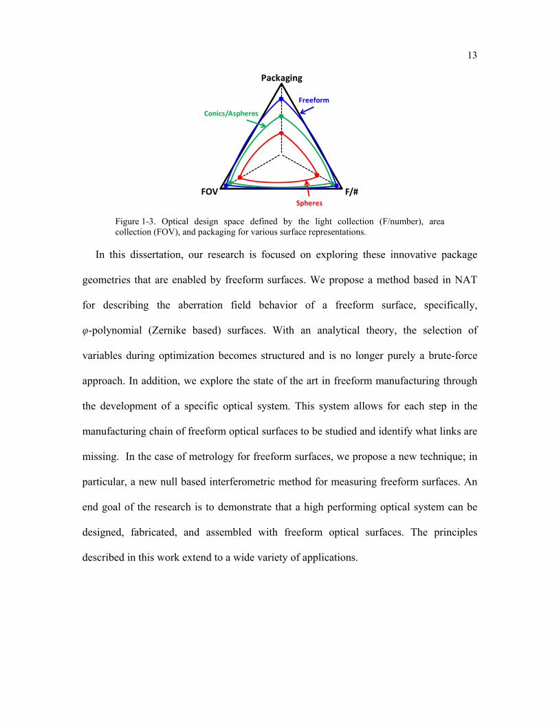
13
F/#FOV
Packaging
Freeform
Spheres
Conics/Aspheres
Figure 1-3. Optical design space defined by the light collection (F/number), area collection (FOV), and packaging for various surface representations.
In this dissertation, our research is focused on exploring these innovative package
geometries that are enabled by freeform surfaces. We propose a method based in NAT
for describing the aberration field behavior of a freeform surface, specifically,
φ-polynomial (Zernike based) surfaces. With an analytical theory, the selection of
variables during optimization becomes structured and is no longer purely a brute-force
approach. In addition, we explore the state of the art in freeform manufacturing through
the development of a specific optical system. This system allows for each step in the
manufacturing chain of freeform optical surfaces to be studied and identify what links are
missing. In the case of metrology for freeform surfaces, we propose a new technique; in
particular, a new null based interferometric method for measuring freeform surfaces. An
end goal of the research is to demonstrate that a high performing optical system can be
designed, fabricated, and assembled with freeform optical surfaces. The principles
described in this work extend to a wide variety of applications.
14
1.4 Dissertation Outline
The dissertation is organized as follows:
Chapter 2 discusses NAT in the context of a perturbed optical system with rotationally
symmetric components. The misalignment induced aberration fields are reviewed through
fifth order with the concept of the aberration field center. Also, the concept of the full
field display, a visualization tool for studying the aberration behavior of a nonsymmetric
optical system, is described.
Chapter 3 presents a method for integrating freeform optical surfaces, specifically
φ-polynomial (Zernike) optical surfaces, into NAT. Using this method, the aberration
fields generated by a Zernike overlay away from the stop surface are derived up to sixth
order and linked to preexisting concepts of NAT. This theory is then applied to a specific
example, three-point mount induced error for both two and three mirror telescopes.
Chapter 4 experimentally validates the extension of NAT to freeform optical surfaces
by measuring the aberration behavior of a specially designed Schmidt telescope. The
Schmidt telescope is composed of two corrector plates, one to remove third order
spherical aberration, and the other to induce an aberration field known as field linear,
field conjugate astigmatism. The generated aberration field is studied under several
conditions including both axial and lateral displacement and rotation of the aberration
generating plate.
Chapter 5 presents the design of an unobscured three mirror imager that utilizes three,
tilted φ-polynomial optical surfaces. The design shows how the concepts derived in NAT
for freeform surfaces can be used to effectively choose variables for optimization. These
15
strategies target either field constant or field dependent aberration correction and utilize
the full field display as an analysis technique.
Chapter 6 demonstrates a new interferometric nulling technique for the measurement
of φ-polynomial optical surfaces. In this method, several adaptable subsystems are
combined that each null an aberration type present in the departure of the mirror surface.
This method is used to design configurations for measuring both convex and concave
optical surfaces. An experimental measurement of an as-fabricated concave,
φ-polynomial optical surface is also demonstrated.
Chapter 7 demonstrates the design and assembly of an optical housing for the optical
system described in Chapter 5. The mechanical housing and its sensitivity to
manufacturing error is studied as well as its susceptibility to stray light. Finally, the
as-built system is presented along with its as-built optical performance.
16
Chapter 2. Aberration Fields for Tilted and Decentered Optical Systems with Rotationally Symmetric Components
The wavefront expansion and surface contributions to the individual aberrations that
describe the imaging properties of an optical system have historically assumed the optical
system is rotationally symmetric [55]. In this case, the third order aberrations are the sum
of the individual surface contributions. For the unobscured reflective systems that were
described in Chapter 1, the symmetry has been broken by either offsetting the aperture or
tilting the optical components. As a result, a new foundation needs to be established that
can handle the imaging behavior of nonsymmetric optical systems.
2.1 Aberration Field Centers
The extension of aberration theory to nonsymmetric optical systems was approached by
Buchroeder [5] in which he proposed that the aberration fields of any optical system are
composed of the contributions of rotationally symmetric surfaces that may be aspheric
where each surface contributes rotationally symmetric aberration fields; however, the
center of the aberration fields will be offset and defined by the surface’s decentration or
tilt. As a result, the net aberration fields are still the summation of the shifted, individual
surface contributions. The shift of the aberration fields is relative to the center of the
Gaussian image plane that is located by the optical axis ray (OAR). The OAR
corresponds to the ray that connects the center of the object, to be chosen arbitrarily, with
the center of the aperture stop in the system [20, 22]. The intersection of the OAR with
the image plane defines the field center for each individual surface’s offset. Buchroeder
introduced a vector, sphjσ , to quantify the shift of the aberration field contributions for a
spherical surface j. Specifically, sphjσ represents a vector that lies in the plane of the image
and points to the intersection of a line that connects the center of curvature and the center
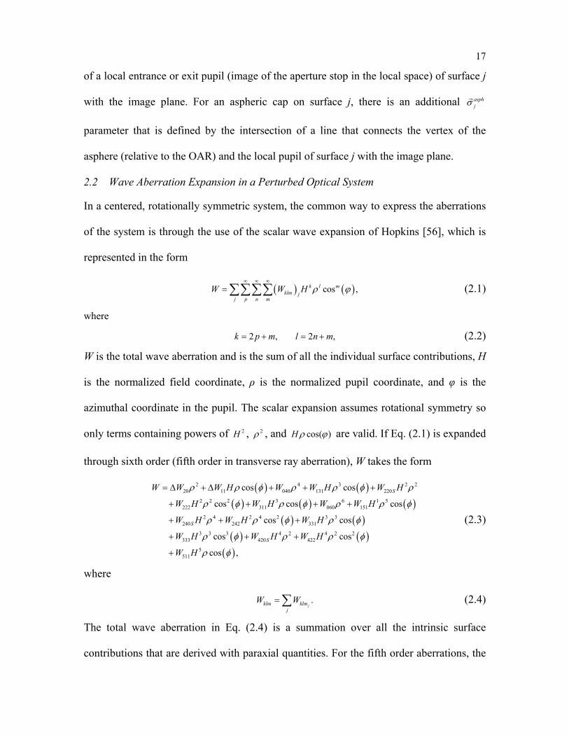
17
of a local entrance or exit pupil (image of the aperture stop in the local space) of surface j
with the image plane. For an aspheric cap on surface j, there is an additional asphjσ
parameter that is defined by the intersection of a line that connects the vertex of the
asphere (relative to the OAR) and the local pupil of surface j with the image plane.
2.2 Wave Aberration Expansion in a Perturbed Optical System
In a centered, rotationally symmetric system, the common way to express the aberrations
of the system is through the use of the scalar wave expansion of Hopkins [56], which is
represented in the form
( ) ( )cos ,k l mklm j
j p n mW W H ρ ϕ
∞ ∞ ∞
= ∑∑∑∑ (2.1)
where
2 , 2 ,k p m l n m= + = + (2.2)
W is the total wave aberration and is the sum of all the individual surface contributions, H
is the normalized field coordinate, ρ is the normalized pupil coordinate, and φ is the
azimuthal coordinate in the pupil. The scalar expansion assumes rotational symmetry so
only terms containing powers of 2H , 2ρ , and cos( )Hρ ϕ are valid. If Eq. (2.1) is expanded
through sixth order (fifth order in transverse ray aberration), W takes the form
( ) ( )( ) ( ) ( )
( ) ( )( ) ( )
( )
2 4 3 2 220 11 040 131 220
2 2 2 3 6 1 5222 311 060 151
2 4 2 4 2 3 3240 242 331
3 3 3 4 2 4 2 2333 420 422
5511
cos cos
cos cos cos
cos cos
cos cos
cos ,
S
S
S
W W W H W W H W H
W H W H W W H
W H W H W H
W H W H W H
W H
ρ ρ φ ρ ρ φ ρ
ρ φ ρ φ ρ ρ φ
ρ ρ φ ρ φ
ρ φ ρ ρ φ
ρ φ
= ∆ + ∆ + + +
+ + + +
+ + +
+ + +
+
(2.3)
where
.jklm klm
jW W= ∑ (2.4)
The total wave aberration in Eq. (2.4) is a summation over all the intrinsic surface
contributions that are derived with paraxial quantities. For the fifth order aberrations, the
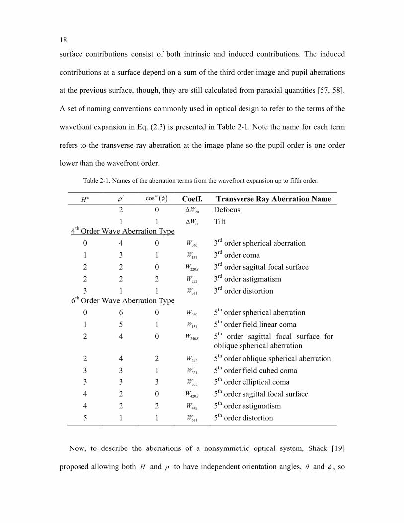
18
surface contributions consist of both intrinsic and induced contributions. The induced
contributions at a surface depend on a sum of the third order image and pupil aberrations
at the previous surface, though, they are still calculated from paraxial quantities [57, 58].
A set of naming conventions commonly used in optical design to refer to the terms of the
wavefront expansion in Eq. (2.3) is presented in Table 2-1. Note the name for each term
refers to the transverse ray aberration at the image plane so the pupil order is one order
lower than the wavefront order.
Table 2-1. Names of the aberration terms from the wavefront expansion up to fifth order.
kH lρ ( )cosm φ Coeff. Transverse Ray Aberration Name 2 0 20W∆ Defocus 1 1 11W∆ Tilt
4th Order Wave Aberration Type 0 4 0 040W 3rd order spherical aberration 1 3 1 131W 3rd order coma 2 2 0 220SW 3rd order sagittal focal surface 2 2 2 222W 3rd order astigmatism 3 1 1 311W 3rd order distortion
6th Order Wave Aberration Type 0 6 0 060W 5th order spherical aberration 1 5 1 151W 5th order field linear coma 2 4 0 240SW 5th order sagittal focal surface for
oblique spherical aberration 2 4 2 242W 5th order oblique spherical aberration 3 3 1 331W 5th order field cubed coma 3 3 3 333W 5th order elliptical coma 4 2 0 420SW 5th order sagittal focal surface 4 2 2 442W 5th order astigmatism 5 1 1 511W 5th order distortion
Now, to describe the aberrations of a nonsymmetric optical system, Shack [19]
proposed allowing both H and ρ to have independent orientation angles, θ and φ , so
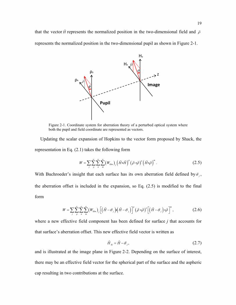
19
that the vector H
represents the normalized position in the two-dimensional field and ρ
represents the normalized position in the two-dimensional pupil as shown in Figure 2-1.
ρx
ρy z
Pupil
Imageφ
θ
ρ
HHx
Hy
Figure 2-1. Coordinate system for aberration theory of a perturbed optical system where both the pupil and field coordinate are represented as vectors.
Updating the scalar expansion of Hopkins to the vector form proposed by Shack, the
representation in Eq. (2.1) takes the following form
( ) ( ) ( ) ( ) .p mn
klm jj p n m
W W H H Hρ ρ ρ∞ ∞ ∞
= ∑∑∑∑
(2.5)
With Buchroeder’s insight that each surface has its own aberration field defined by jσ ,
the aberration offset is included in the expansion, so Eq. (2.5) is modified to the final
form
( ) ( ) ( ) ( ) ( ) ,p mn
klm j j jjj p n m
W W H H Hσ σ ρ ρ σ ρ∞ ∞ ∞
= − − − ∑∑∑∑
(2.6)
where a new effective field component has been defined for surface j that accounts for
that surface’s aberration offset. This new effective field vector is written as
,Aj jH H σ= −
(2.7)
and is illustrated at the image plane in Figure 2-2. Depending on the surface of interest,
there may be an effective field vector for the spherical part of the surface and the aspheric
cap resulting in two contributions at the surface.
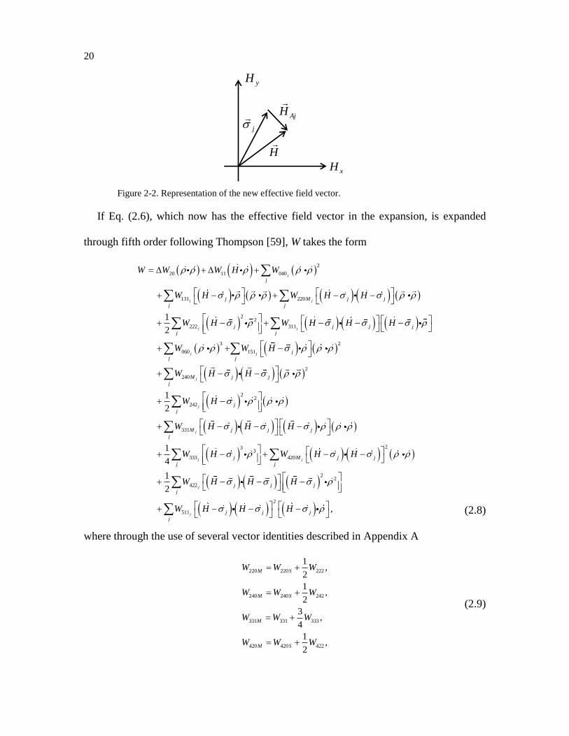
20
H
j AjH
xH
yH
Figure 2-2. Representation of the new effective field vector.
If Eq. (2.6), which now has the effective field vector in the expansion, is expanded
through fifth order following Thompson [59], W takes the form
2
20 11 040
131 220
22
222 311
3 2
060 151
1
2
j
j j
j j
j j
j
j M j j
j j
j j j j
j j
j
j j
W W W H W
W H W H H
W H W H H H
W W H
W
2
240
22
242
331
233
333 420
2
422
1
2
1
4
1
2
j
j
j
j j
j
M j j
j
j
j
M j j j
j
j M j j
j j
j j j
j
H H
W H
W H H H
W H W H H
W H H H
2
2
511 ,j j j j
j
W H H H
(2.8)
where through the use of several vector identities described in Appendix A
220 220 222
240 240 242
331 331 333
420 420 422
1,
2
1,
2
3,
4
1,
2
M S
M S
M
M S
W W W
W W W
W W W
W W W
(2.9)
21
have been defined. The identities used to arrive at the terms in Eq. (2.9) and the final
wavefront expansion in Eq. (2.8) have made use of an operation known as vector
multiplication. This operation is essential to represent the aberration fields of
nonsymmetric optical systems and can be thought of as an extension to the mathematics
of complex numbers. The properties of vector multiplication are described in more detail
in Thompson [20, 59] and are summarized in Appendix A. Also, it is important to
re-emphasize that the aberration surface contributions observed in Eq. (2.9) are not
affected by a perturbation because they are functions of paraxial quantities.
Though Eq. (2.8) is complete, it does not provide any insight into the behavior of the
aberrations in a nonsymmetric optical system. This behavior is revealed by performing a
summation over the surfaces to get the total aberration effect. To simplify the notation,
Thompson [59] proposed using substitutions for the summations as follows
( )
( )
( )
( )
( )
2 2
3 3
2
2 2
2,
j
j
j
j
j
j
j
j
klm klm jj
klm klm j jj
klm klm jj
klm klm j j jj
klm klm jj
klm klm j jj
klm klm j j jj
klm klm j j jj
A W
B W
B W
C W
C W
D W
D W
E W
σ
σ σ
σ
σ σ σ
σ
σ σ
σ σ σ
σ σ σ
=
=
=
=
=
=
=
=
∑
∑
∑
∑
∑
∑
∑
∑
(2.10)
creating a set of image plane perturbation vectors that are only created when the
symmetry of the optical system is broken. With the perturbation vectors defined, the
wavefront expansion in Eq. (2.8) is expanded further and simplified following
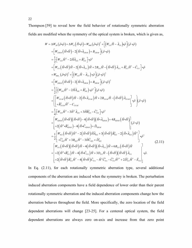
22
Thompson [59] to reveal how the field behavior of rotationally symmetric aberration
fields are modified when the symmetry of the optical system is broken, which is given as,
( ) ( ) ( ) ( ) ( )
( ) ( ) ( )
( ) ( ) ( )
220 11 040 131 131
220 220 220
2 2 2222 222 222
2 *311 311 311 311 311 311
060
2
1 22
2 2
j
M M M
W W W H W W H A
W H H H A B
W H HA B
W H H H H A H B H H H A B H C
W
ρ ρ ρ ρ ρ ρ ρ ρ
ρ ρ
ρ
ρ
= ∆ + ∆ + + − + − +
+ − +
+ − + − + −
+
( ) ( ) ( )
( ) ( ) ( )
( ) ( )
( ) ( ) ( ) ( )
3 2151 151
2240 240 240
2 2 2242 242 242
331 331 331 331
2 *331 331
2
1 22
2 2
14
M M M
M M M M
M M
W H A
W H H H A B
W H HA B
W H H H H A H B H H H A
B H C
ρ ρ ρ ρ ρ
ρ ρ
ρ ρ ρ
ρ ρ ρ
+ − + − +
+ − +
− + − + + −
+
( )( ) ( )( ) ( )( ) ( )
( )
( ) ( ) ( ) ( )
3 2 2 3 3333 333 333 333
420 420 420
2 2420 420 420
2 2 2422 422 422 422
3 *422
3 3
4 4
2 4
2 3 212 3
M M M
M M M
W H H A HB C
W H H H H H H H A B H H
H B H C D
W H H H H H HA H H B H A H
C H B
ρ
ρ ρ
− + −
− + + + − +
− + −+
− +
( )( ) ( )( ) ( )( ) ( ) ( )( )( ) ( )
2
2 2422 422 422
511 511 511
2 2511 511 511 511
2 * 2 * 3 2* 2 *511 511 511 511 511 511
3
4 6
2 4 3
2 4 2
H HC D
W H H H H H H H H A H B H H H
H B H H C H D H H H H H A
H H B H H H C H C C H D H E
ρ − +
− +
+ + − + −
+ − − − + −
.ρ
(2.11)
In Eq. (2.11), for each rotationally symmetric aberration type, several additional
components of the aberration are induced when the symmetry is broken. The perturbation
induced aberration components have a field dependence of lower order than their parent
rotationally symmetric aberration and the induced aberration components change how the
aberration behaves throughout the field. More specifically, the zero location of the field
dependent aberrations will change [23-25]. For a centered optical system, the field
dependent aberrations are always zero on-axis and increase from that zero point
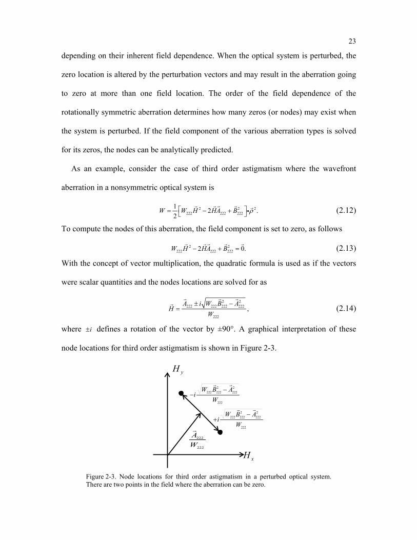
23
depending on their inherent field dependence. When the optical system is perturbed, the
zero location is altered by the perturbation vectors and may result in the aberration going
to zero at more than one field location. The order of the field dependence of the
rotationally symmetric aberration determines how many zeros (or nodes) may exist when
the system is perturbed. If the field component of the various aberration types is solved
for its zeros, the nodes can be analytically predicted.
As an example, consider the case of third order astigmatism where the wavefront
aberration in a nonsymmetric optical system is
2 2 2222 222 222
1 2 .2
W W H HA B ρ = − +
(2.12)
To compute the nodes of this aberration, the field component is set to zero, as follows
2 2222 222 2222 0.W H HA B− + =
(2.13)
With the concept of vector multiplication, the quadratic formula is used as if the vectors
were scalar quantities and the nodes locations are solved for as
2 2
222 222 222 222
222
,A i W B A
HW
± −=
(2.14)
where i± defines a rotation of the vector by ±90°. A graphical interpretation of these
node locations for third order astigmatism is shown in Figure 2-3.
xH
yH
2 2222 222 222
222
W B Ai
W−
+
222
222
AW
2 2222 222 222
222
W B Ai
W−
−
Figure 2-3. Node locations for third order astigmatism in a perturbed optical system. There are two points in the field where the aberration can be zero.
24
In addition to the general case, there are several special cases to be addressed for this
aberration as well. The first case is when the system is corrected for third order
astigmatism, that is, 222 0W = . In this case, the wavefront aberration becomes
2 2222 222
1 2 .2
W HA B ρ = − +
(2.15)
If both 222A
and 2222B
are non-zero, the aberration takes the form of linear astigmatism (i.e.
astigmatism that depends linearly with field) and a node will exist at
2222
222
.2BHA
=
(2.16)
Lastly, if 222 0W = and 222 0A =
then the wavefront aberration becomes
2 2222
1 ,2
W B ρ=
(2.17)
where the astigmatism is constant throughout the field in both magnitude and orientation
and governed by 2222B
. Similar methodology is applied for the other aberrations to reveal
their characteristic behavior throughout the field and to analytically determine their node
locations for different tilt and decenter perturbations as detailed in [23-25].
2.3 Full Field Aberration Display
In a centered optical system with rotationally symmetric components, the aberrations
need only be assessed in one field direction (historically, the +y-field). With the
aberrations known in this field direction, they are also known in every other field
direction since the aberrations will also be rotationally symmetric. In most optical design
software packages, a common way to assess the aberration performance is through a
transverse ray aberration plot. In this plot, the transverse ray aberration is computed as a
function of pupil position for various field heights along one field direction. This plot is
useful for rotationally symmetric systems, but if the optical system symmetry is broken,
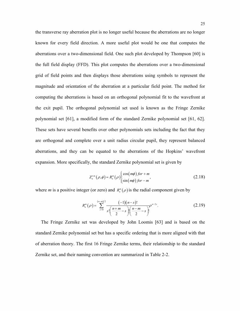
25
the transverse ray aberration plot is no longer useful because the aberrations are no longer
known for every field direction. A more useful plot would be one that computes the
aberrations over a two-dimensional field. One such plot developed by Thompson [60] is
the full field display (FFD). This plot computes the aberrations over a two-dimensional
grid of field points and then displays those aberrations using symbols to represent the
magnitude and orientation of the aberration at a particular field point. The method for
computing the aberrations is based on an orthogonal polynomial fit to the wavefront at
the exit pupil. The orthogonal polynomial set used is known as the Fringe Zernike
polynomial set [61], a modified form of the standard Zernike polynomial set [61, 62].
These sets have several benefits over other polynomials sets including the fact that they
are orthogonal and complete over a unit radius circular pupil, they represent balanced
aberrations, and they can be equated to the aberrations of the Hopkins’ wavefront
expansion. More specifically, the standard Zernike polynomial set is given by
( ) ( )( )( )
cos, ,
sinm m
n n
m for mZ R
m for m
φρ φ ρ
φ±
+= −
(2.18)
where m is a positive integer (or zero) and ( )mnR ρ is the radial component given by
( ) ( )( )( ) 22
0
1 !.
! ! !2 2
n mm n sn
s
n sR
n m n ms s sρ ρ
−−
=
− −=
+ − − −
∑ (2.19)
The Fringe Zernike set was developed by John Loomis [63] and is based on the
standard Zernike polynomial set but has a specific ordering that is more aligned with that
of aberration theory. The first 16 Fringe Zernike terms, their relationship to the standard
Zernike set, and their naming convention are summarized in Table 2-2.
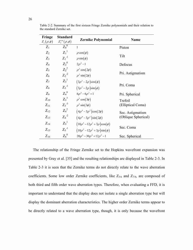
26
Table 2-2. Summary of the first sixteen Fringe Zernike polynomials and their relation to the standard Zernike set.
Fringe ( ),jZ ρ φ
Standard ( ),m
nZ ρ φ± Zernike Polynomial Name
Z1 Z00 1 Piston
Z2 Z11 ( )cosρ φ
Tilt Z3 Z1-1 ( )sinρ φ
Z4 Z20 22 1ρ − Defocus
Z5 Z22 ( )2 cos 2ρ φ
Pri. Astigmatism Z6 Z2-2 ( )2 sin 2ρ φ
Z7 Z31 ( ) ( )33 2 cosρ ρ φ−
Pri. Coma Z8 Z3-1 ( ) ( )33 2 sinρ ρ φ−
Z9 Z40 4 26 6 1ρ ρ− + Pri. Spherical
Z10 Z33 ( )3 cos 3ρ φ Trefoil
(Elliptical Coma) Z11 Z3-3 ( )3 sin 3ρ φ
Z12 Z42 ( ) ( )4 24 3 cos 2ρ ρ φ− Sec. Astigmatism
(Oblique Spherical) Z13 Z4-2 ( ) ( )4 24 3 sin 2ρ ρ φ−
Z14 Z51 ( ) ( )5 310 12 3 cosρ ρ ρ φ− +
Sec. Coma Z15 Z5-1 ( ) ( )5 310 12 3 sinρ ρ ρ φ− +
Z16 Z60 6 4 220 30 12 1ρ ρ ρ− + − Sec. Spherical
The relationship of the Fringe Zernike set to the Hopkins wavefront expansion was
presented by Gray et al. [35] and the resulting relationships are displayed in Table 2-3. In
Table 2-3 it is seen that the Zernike terms do not directly relate to the wave aberration
coefficients. Some low order Zernike coefficients, like Z5/6 and Z7/8, are composed of
both third and fifth order wave aberration types. Therefore, when evaluating a FFD, it is
important to understand that the display does not isolate a single aberration type but will
display the dominant aberration characteristics. The higher order Zernike terms appear to
be directly related to a wave aberration type, though, it is only because the wavefront
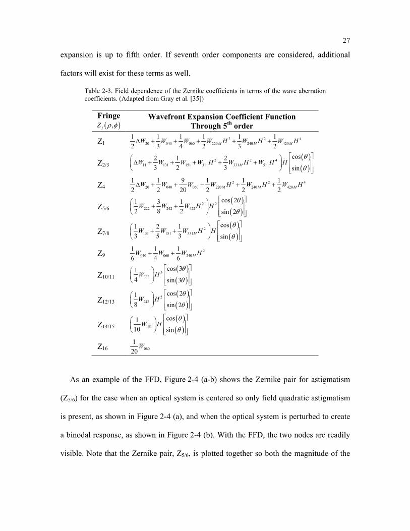
27
expansion is up to fifth order. If seventh order components are considered, additional
factors will exist for these terms as well.
Table 2-3. Field dependence of the Zernike coefficients in terms of the wave aberration coefficients. (Adapted from Gray et al. [35])
Fringe ( ),jZ ρ φ
Wavefront Expansion Coefficient Function Through 5th order
Z1 2 2 420 040 060 220 240 420
1 1 1 1 1 12 3 4 2 3 2M M MW W W W H W H W H∆ + + + + +
Z2/3 ( )( )
2 2 411 131 151 311 331 511
cos2 1 23 2 3 sinMW W W W H W H W H H
θ
θ
∆ + + + + +
Z4 2 2 420 040 060 220 240 420
1 1 9 1 1 12 2 20 2 2 2M M MW W W W H W H W H∆ + + + + +
Z5/6 ( )( )
2 2222 242 422
cos 21 3 12 8 2 sin 2
W W W H Hθ
θ
+ +
Z7/8 ( )( )
2131 151 331
cos1 2 13 5 3 sinMW W W H H
θ
θ
+ +
Z9 2040 060 240
1 1 16 4 6 MW W W H+ +
Z10/11 ( )( )
3333
cos 314 sin 3
W Hθ
θ
Z12/13 ( )( )
2242
cos 218 sin 2
W Hθ
θ
Z14/15 ( )( )151
cos110 sin
W Hθ
θ
Z16 060120
W
As an example of the FFD, Figure 2-4 (a-b) shows the Zernike pair for astigmatism
(Z5/6) for the case when an optical system is centered so only field quadratic astigmatism
is present, as shown in Figure 2-4 (a), and when the optical system is perturbed to create
a binodal response, as shown in Figure 2-4 (b). With the FFD, the two nodes are readily
visible. Note that the Zernike pair, Z5/6, is plotted together so both the magnitude of the
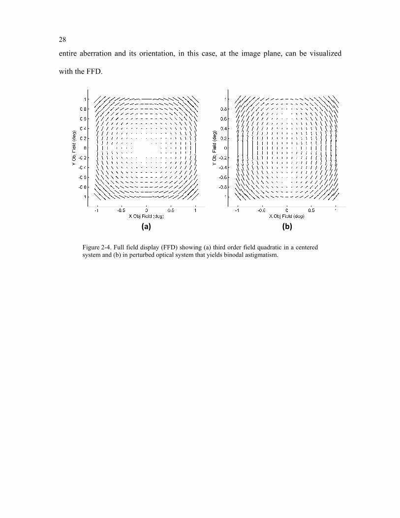
28
entire aberration and its orientation, in this case, at the image plane, can be visualized
with the FFD.
(a) (b)
Figure 2-4. Full field display (FFD) showing (a) third order field quadratic in a centered system and (b) in perturbed optical system that yields binodal astigmatism.
29
Chapter 3. Aberration Fields in Optical Systems with φ-Polynomial Optical Surfaces
Nodal aberration theory (NAT) describes the aberration fields of optical systems when
the constraint of rotational symmetry is not imposed. Historically the theory, discovered
by Shack [19] and developed by Thompson [20], has been limited to optical imaging
systems made of rotationally symmetric components, or offset aperture portions thereof,
that are tilted and/or decentered. Recently, the special case of an astigmatic optical
surface located at the aperture stop (or pupil) was introduced into NAT by
Schmid et al. [64] and analyzed for the case of a primary mirror in a two mirror
telescope. At the stop surface, the beam footprint is the same for all field points, so all
field angles receive the same contribution from the astigmatic surface. The net astigmatic
field dependence, as predicted by NAT, and as validated by real ray tracing, takes on
characteristic nodal features that allow the presence and magnitude/orientation of
astigmatic figure error to be readily distinguished from the presence and
magnitude/orientation of any misalignment of the secondary mirror.
In this chapter, a path based in NAT is presented for developing an analytic theory for
the aberration fields of nonsymmetric optical systems with freeform surfaces. With this
extension to NAT, the zeros (or nodes) of the aberration contributions, which are
distributed throughout the FOV, can be anticipated analytically and targeted directly for
the correction or control of the aberrations in an optical system with freeform surfaces.
We consider an optical surface defined by a conic plus a ϕ-polynomial overlay, where the
sag of the overlay depends on the radial component, ρ, as well as the azimuthal
component, φ, within the aperture of the surface. Significantly, the freeform overlay can
be placed anywhere within the optical imaging system. Under these more general
30
conditions, it will be shown that the aberration contributions of the freeform surface
contribute both field constant and field dependent terms to the net aberration field of the
optical system. These aberration terms are derived for a specific ϕ-polynomial set, the
Zernike polynomial set up to sixth order. For each term in this subset, the aberration
behavior throughout the field is examined. Unexpectedly, we find that the impact of
integrating ϕ-polynomial freeform surfaces into NAT does not introduce new forms of
field dependence; rather, the freeform parameters link directly with the terms presented
for the generally multinodal field dependence of the sixth order wavefront aberrations
derived for tilted and decentered rotationally symmetric surfaces as reviewed in
Chapter 2. As an example of the types of analyses that can now be carried out with NAT,
the impact of three point mount-induced error (trefoil) on the field dependence of
astigmatism is presented here.
3.1 Formulating Nodal Aberration Theory for Freeform, ϕ-Polynomial Surfaces away from the Aperture Stop
To analytically characterize the impact of a ϕ-polynomial optical surface away from the
stop on the net aberration field, first consider a classical Schmidt telescope configuration.
The telescope is composed of a rotationally symmetric third order (fourth order in
wavefront) aspheric corrector plate in coincidence with a mechanical aperture that is the
stop of the optical system, located at the center of curvature of a spherical mirror. In such
a configuration, the net aberration contribution of the aspheric corrector plate, ,Corrector StopW ,
is described by the overall third order spherical aberration it induces, given by
( ) ( )2, 040
ASPHCorrector StopW W ρ ρ=
(3.1)
31
where ( )040
ASPHW denotes the spherical aberration wave aberration contribution from the
aspheric corrector plate and ρ is a normalized two-dimensional pupil vector that denotes
a location in the pupil of the Schmidt telescope.
Nominally, the Schmidt telescope is corrected for third order spherical aberration by
the corrector plate and for third order coma and astigmatism by locating the stop at the
center of curvature of the spherical mirror, leaving only field curvature as the limiting
third order aberration. The case where an aspheric corrector plate located at the stop or
pupil of an optical system is decentered from the optical axis was previously treated in
the context of NAT by Thompson [65] and was more recently revisited by
Wang et al. [66]. If the aspheric plate is instead shifted axially (i.e. longitudinally along
the optical axis) relative to a physical aperture stop, as shown in Figure 3-1 (a), the beam
for any off-axis field point will begin to displace across the aspheric plate. The amount of
relative beam displacement, h∆
, is given by
,y uth H Hy y
∆ ≡ =
(3.2)
where y is the paraxial marginal ray height on the aspheric plate, y is the paraxial chief
ray height on the aspheric plate, u is the paraxial chief ray angle, t is the distance between
the aspheric corrector plate and the mechanical aperture that is the optical system stop,
and H
is the normalized two-dimensional field vector that locates the field point of
interest in the image plane (i.e. 0≤| H
|≤1).
Conceptually, the beam displacement on the corrector plate when it is shifted away
from the stop can be thought of as a field dependent decenter of the aspheric corrector
when it is located at the aperture stop as shown in Figure 3-1 (b) where the mapping of
32
the normalized pupil coordinate is modified from ρ to 'ρ . Therefore, the net aberration
contribution of the aspheric corrector described by Eq. (3.1) must be modified to account
for this effect. By replacing ρ with ' hρ + ∆
and expanding the pupil dependence leads to
a modified aberration contribution, ,Corrector Not StopW , that is given by
( ) ( ) ( )
( )( ) ( )( ) ( )( )
( ) ( )( ) ( )
2
, 040
2
040 22 2
' '
4 4,
2 4
ASPHCorrector Not Stop
ASPH
W W h h
h h hW
h h h h h h
ρ ρ
ρ ρ ρ ρ ρ ρ ρ
ρ ρ
= + ∆ + ∆ + ∆ + ∆ ∆ = + ∆ + ∆ ∆ ∆ + ∆ ∆
(3.3)
where it is recognized that the measurement is done in the shifted pupil coordinate and
the primes have been dropped from the final expression of Eq. (3.3). As can be seen from
Eq. (3.3), the original spherical aberration contribution from the aspheric plate generates
lower order field dependent aberration components as the plate is shifted away from the
stop. Note that the operation of vector multiplication, introduced in [20], is being used in
this expansion. The aberration terms that are generated by this expansion are the
conventional third order field aberration terms summarized in Table 3-1, which could be
anticipated since the field aberrations are the product of spherical aberration in the
presence of a stop shift from the center of curvature.
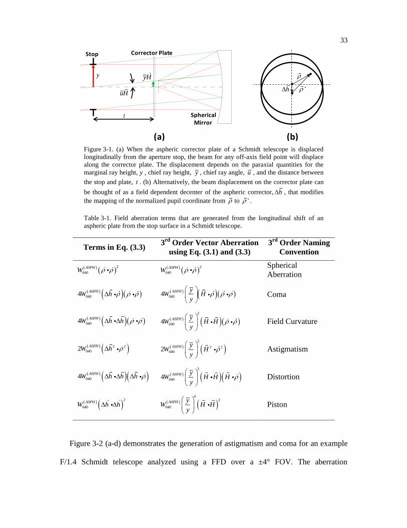
33
16:56:15
Flat-field Schmidt Scale: 0.80 ORA 12-Jun-12
31.25 MM
yHy
t
uH
Stop Corrector Plate
SphericalMirror
h '
(a) (b)
Figure 3-1. (a) When the aspheric corrector plate of a Schmidt telescope is displaced
longitudinally from the aperture stop, the beam for any off-axis field point will displace
along the corrector plate. The displacement depends on the paraxial quantities for the
marginal ray height, y , chief ray height,
y , chief ray angle, u , and the distance between
the stop and plate, t . (b) Alternatively, the beam displacement on the corrector plate can
be thought of as a field dependent decenter of the aspheric corrector, h , that modifies
the mapping of the normalized pupil coordinate from to ' .
Table 3-1. Field aberration terms that are generated from the longitudinal shift of an
aspheric plate from the stop surface in a Schmidt telescope.
Terms in Eq. (3.3) 3
rd Order Vector Aberration
using Eq. (3.1) and (3.3)
3rd
Order Naming
Convention
2
040
ASPHW
2
040
ASPHW
Spherical
Aberration
0404ASPH
W h 0404ASPH y
W Hy
Coma
0404ASPH
W h h 2
0404ASPH y
W H Hy
Field Curvature
2 2
0402ASPH
W h 2
2 2
0402ASPH y
W Hy
Astigmatism
0404ASPH
W h h h 3
0404ASPH y
W H H Hy
Distortion
2
040
ASPHW h h
42
040
ASPH yW H H
y
Piston
Figure 3-2 (a-d) demonstrates the generation of astigmatism and coma for an example
F/1.4 Schmidt telescope analyzed using a FFD over a ±4° FOV. The aberration
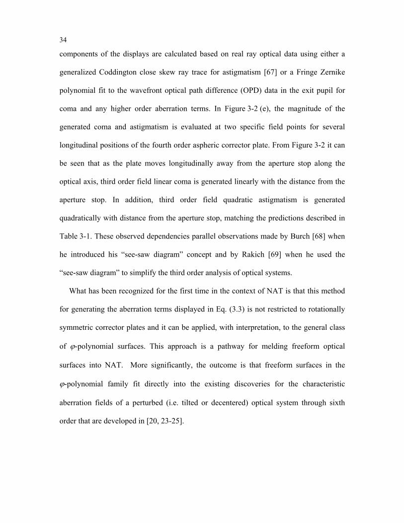
34
components of the displays are calculated based on real ray optical data using either a
generalized Coddington close skew ray trace for astigmatism [67] or a Fringe Zernike
polynomial fit to the wavefront optical path difference (OPD) data in the exit pupil for
coma and any higher order aberration terms. In Figure 3-2 (e), the magnitude of the
generated coma and astigmatism is evaluated at two specific field points for several
longitudinal positions of the fourth order aspheric corrector plate. From Figure 3-2 it can
be seen that as the plate moves longitudinally away from the aperture stop along the
optical axis, third order field linear coma is generated linearly with the distance from the
aperture stop. In addition, third order field quadratic astigmatism is generated
quadratically with distance from the aperture stop, matching the predictions described in
Table 3-1. These observed dependencies parallel observations made by Burch [68] when
he introduced his “see-saw diagram” concept and by Rakich [69] when he used the
“see-saw diagram” to simplify the third order analysis of optical systems.
What has been recognized for the first time in the context of NAT is that this method
for generating the aberration terms displayed in Eq. (3.3) is not restricted to rotationally
symmetric corrector plates and it can be applied, with interpretation, to the general class
of ϕ-polynomial surfaces. This approach is a pathway for melding freeform optical
surfaces into NAT. More significantly, the outcome is that freeform surfaces in the
ϕ-polynomial family fit directly into the existing discoveries for the characteristic
aberration fields of a perturbed (i.e. tilted or decentered) optical system through sixth
order that are developed in [20, 23-25].
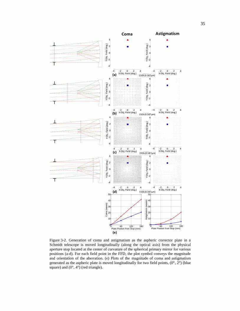
35
08:36:17
Flat-field Schmidt
ORA 30-May-12
ASTIGMATIC LINE IMAGE
vs
FIELD ANGLE IN OBJECT SPACE
Minimum = 0
Maximum = 0.55844
Average = 0.19928
Std Dev = 0.12784
1.992mm
-4 -2 0 2 4
X Field Angle in Object Space - degrees
-4
-2
0
2
4
Y Field Angle in Object Space - degrees
08:36:21
Flat-field Schmidt
ORA 30-May-12
FRINGE ZERNIKE PAIR Z7 AND Z8
vs
FIELD ANGLE IN OBJECT SPACE
Minimum = 0.10098e-10
Maximum = 58.486
Average = 33.692
Std Dev = 12.373
150waves ( 587.6 nm)
-4 -2 0 2 4
X Field Angle in Object Space - degrees
-4
-2
0
2
4
Y Field Angle in Object Space - degrees
08:36:17
Flat-field Schmidt ORA 30-May-12
25.00 MM
Y O
bj.
Fie
ld (
de
g.)
4
2
0
-2
-4
Y O
bj.
Fie
ld (
de
g.)
4
2
0
-2
-4
08:36:04
Flat-field Schmidt ORA 30-May-12
25.00 MM
08:36:04
Flat-field Schmidt
ORA 30-May-12
ASTIGMATIC LINE IMAGE
vs
FIELD ANGLE IN OBJECT SPACE
Minimum = 0
Maximum = 0.24281
Average = 0.08755
Std Dev = 0.055768
1.992mm
-4 -2 0 2 4
X Field Angle in Object Space - degrees
-4
-2
0
2
4
Y Field Angle in Object Space - degrees
08:36:08
Flat-field Schmidt
ORA 30-May-12
FRINGE ZERNIKE PAIR Z7 AND Z8
vs
FIELD ANGLE IN OBJECT SPACE
Minimum = 0.89056e-12
Maximum = 40.116
Average = 22.744
Std Dev = 8.4663
150waves ( 587.6 nm)
-4 -2 0 2 4
X Field Angle in Object Space - degrees
-4
-2
0
2
4
Y Field Angle in Object Space - degrees
Y O
bj.
Fie
ld (
de
g.)
4
2
0
-2
-4
Y O
bj.
Fie
ld (
de
g.)
4
2
0
-2
-408:35:51
Flat-field Schmidt
ORA 30-May-12
ASTIGMATIC LINE IMAGE
vs
FIELD ANGLE IN OBJECT SPACE
Minimum = 0
Maximum = 0.060055
Average = 0.021751
Std Dev = 0.013804
1.992mm
-4 -2 0 2 4
X Field Angle in Object Space - degrees
-4
-2
0
2
4
Y Field Angle in Object Space - degrees
08:35:55
Flat-field Schmidt
ORA 30-May-12
FRINGE ZERNIKE PAIR Z7 AND Z8
vs
FIELD ANGLE IN OBJECT SPACE
Minimum = 0.92121e-13
Maximum = 19.979
Average = 11.303
Std Dev = 4.2147
150waves ( 587.6 nm)
-4 -2 0 2 4
X Field Angle in Object Space - degrees
-4
-2
0
2
4
Y Field Angle in Object Space - degrees
16:17:34
Flat-field Schmidt ORA 29-May-12
25.00 MM
Y O
bj.
Fie
ld (
de
g.)
4
2
0
-2
-4
Y O
bj.
Fie
ld (
de
g.)
4
2
0
-2
-4
08:35:42
Flat-field Schmidt
ORA 30-May-12
FRINGE ZERNIKE PAIR Z7 AND Z8
vs
FIELD ANGLE IN OBJECT SPACE
Minimum = 0.3321e-11
Maximum = 0.40548
Average = 0.2324
Std Dev = 0.08561
150waves ( 587.6 nm)
-4 -2 0 2 4
X Field Angle in Object Space - degrees
-4
-2
0
2
4
Y Field Angle in Object Space - degrees
08:35:39
Flat-field Schmidt
ORA 30-May-12
ASTIGMATIC LINE IMAGE
vs
FIELD ANGLE IN OBJECT SPACE
Minimum = 0
Maximum = 0.28862e-4
Average = 0.10046e-4
Std Dev = 0.65357e-5
1.992mm
-4 -2 0 2 4
X Field Angle in Object Space - degrees
-4
-2
0
2
4
Y Field Angle in Object Space - degrees
16:17:22
Flat-field Schmidt ORA 29-May-12
25.00 MM
Coma Astigmatism
Y O
bj.
Fie
ld (
de
g.)
4
2
0
-2
-4
Y O
bj.
Fie
ld (
de
g.)
4
2
0
-2
-4
X Obj. Field (deg.)-4 -2 0 2 4
X Obj. Field (deg.)-4 -2 0 2 4
X Obj. Field (deg.)-4 -2 0 2 4
X Obj. Field (deg.)-4 -2 0 2 4
X Obj. Field (deg.)-4 -2 0 2 4
X Obj. Field (deg.)-4 -2 0 2 4
X Obj. Field (deg.)-4 -2 0 2 4
X Obj. Field (deg.)-4 -2 0 2 4
(a) 150λ (0.587µm)
09:17:02
Flat-field Schmidt
ORA 12-Jan-12
FRINGE ZERNIKE PAIR Z7 AND Z8
vs
FIELD ANGLE IN OBJECT SPACE
Minimum = 0.55999
Maximum = 0.57967
Average = 0.56928
Std Dev = 0.0057599
4waves ( 587.6 nm)
-4 -2 0 2 4
X Field Angle in Object Space - degrees
-4
-2
0
2
4
Y Field Angle in Object Space - degrees
150λ (0.587µm)
09:17:02
Flat-field Schmidt
ORA 12-Jan-12
FRINGE ZERNIKE PAIR Z7 AND Z8
vs
FIELD ANGLE IN OBJECT SPACE
Minimum = 0.55999
Maximum = 0.57967
Average = 0.56928
Std Dev = 0.0057599
4waves ( 587.6 nm)
-4 -2 0 2 4
X Field Angle in Object Space - degrees
-4
-2
0
2
4
Y Field Angle in Object Space - degrees
(b)
150λ (0.587µm)
09:17:02
Flat-field Schmidt
ORA 12-Jan-12
FRINGE ZERNIKE PAIR Z7 AND Z8
vs
FIELD ANGLE IN OBJECT SPACE
Minimum = 0.55999
Maximum = 0.57967
Average = 0.56928
Std Dev = 0.0057599
4waves ( 587.6 nm)
-4 -2 0 2 4
X Field Angle in Object Space - degrees
-4
-2
0
2
4
Y Field Angle in Object Space - degrees
(c)
(d) 150λ (0.587µm)
09:17:02
Flat-field Schmidt
ORA 12-Jan-12
FRINGE ZERNIKE PAIR Z7 AND Z8
vs
FIELD ANGLE IN OBJECT SPACE
Minimum = 0.55999
Maximum = 0.57967
Average = 0.56928
Std Dev = 0.0057599
4waves ( 587.6 nm)
-4 -2 0 2 4
X Field Angle in Object Space - degrees
-4
-2
0
2
4
Y Field Angle in Object Space - degrees
(e)
0 60 120 1800
10
20
30
40
50
Plate Postion from Stop (mm)
Astigm
atism
(w
aves)
0 60 120 1800
10
20
30
40
50
Plate Postion from Stop (mm)
Com
a (
waves)
Figure 3-2. Generation of coma and astigmatism as the aspheric corrector plate in a
Schmidt telescope is moved longitudinally (along the optical axis) from the physical
aperture stop located at the center of curvature of the spherical primary mirror for various
positions (a-d). For each field point in the FFD, the plot symbol conveys the magnitude
and orientation of the aberration. (e) Plots of the magnitude of coma and astigmatism
generated as the aspheric plate is moved longitudinally for two field points, (0°, 2°) (blue
square) and (0°, 4°) (red triangle).
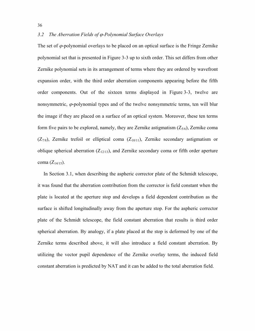
36
3.2 The Aberration Fields of ϕ-Polynomial Surface Overlays
The set of ϕ-polynomial overlays to be placed on an optical surface is the Fringe Zernike
polynomial set that is presented in Figure 3-3 up to sixth order. This set differs from other
Zernike polynomial sets in its arrangement of terms where they are ordered by wavefront
expansion order, with the third order aberration components appearing before the fifth
order components. Out of the sixteen terms displayed in Figure 3-3, twelve are
nonsymmetric, ϕ-polynomial types and of the twelve nonsymmetric terms, ten will blur
the image if they are placed on a surface of an optical system. Moreover, these ten terms
form five pairs to be explored, namely, they are Zernike astigmatism (Z5/6), Zernike coma
(Z7/8), Zernike trefoil or elliptical coma (Z10/11), Zernike secondary astigmatism or
oblique spherical aberration (Z12/13), and Zernike secondary coma or fifth order aperture
coma (Z14/15).
In Section 3.1, when describing the aspheric corrector plate of the Schmidt telescope,
it was found that the aberration contribution from the corrector is field constant when the
plate is located at the aperture stop and develops a field dependent contribution as the
surface is shifted longitudinally away from the aperture stop. For the aspheric corrector
plate of the Schmidt telescope, the field constant aberration that results is third order
spherical aberration. By analogy, if a plate placed at the stop is deformed by one of the
Zernike terms described above, it will also introduce a field constant aberration. By
utilizing the vector pupil dependence of the Zernike overlay terms, the induced field
constant aberration is predicted by NAT and it can be added to the total aberration field.
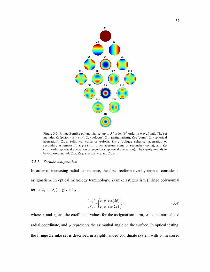
37
Z1
Z3 Z2
Z5Z4
Z8 Z10
Z6
Z12
Z11 Z7
Z9Z13
Z16
Z14Z15
Figure 3-3. Fringe Zernike polynomial set up to 5th order (6th order in wavefront). The set includes Z1 (piston), Z2/3 (tilt), Z4 (defocus), Z5/6 (astigmatism), Z7/8 (coma), Z9 (spherical aberration), Z10/11 (elliptical coma or trefoil), Z12/13 (oblique spherical aberration or secondary astigmatism), Z14/15 (fifth order aperture coma or secondary coma), and Z16 (fifth order spherical aberration or secondary spherical aberration). The φ-polynomials to be explored include Z5/6, Z7/8, Z10/11, Z12/13, and Z14/15.
3.2.1 Zernike Astigmatism
In order of increasing radial dependence, the first freeform overlay term to consider is
astigmatism. In optical metrology terminology, Zernike astigmatism (Fringe polynomial
terms 5Z and 6Z ) is given by
( )( )
255
26 6
cos 2,
sin 2
zZZ z
ρ φ
ρ φ
=
(3.4)
where 5z and 6z are the coefficient values for the astigmatism term, ρ is the normalized
radial coordinate, and φ represents the azimuthal angle on the surface. In optical testing,
the Fringe Zernike set is described in a right-handed coordinate system with φ measured
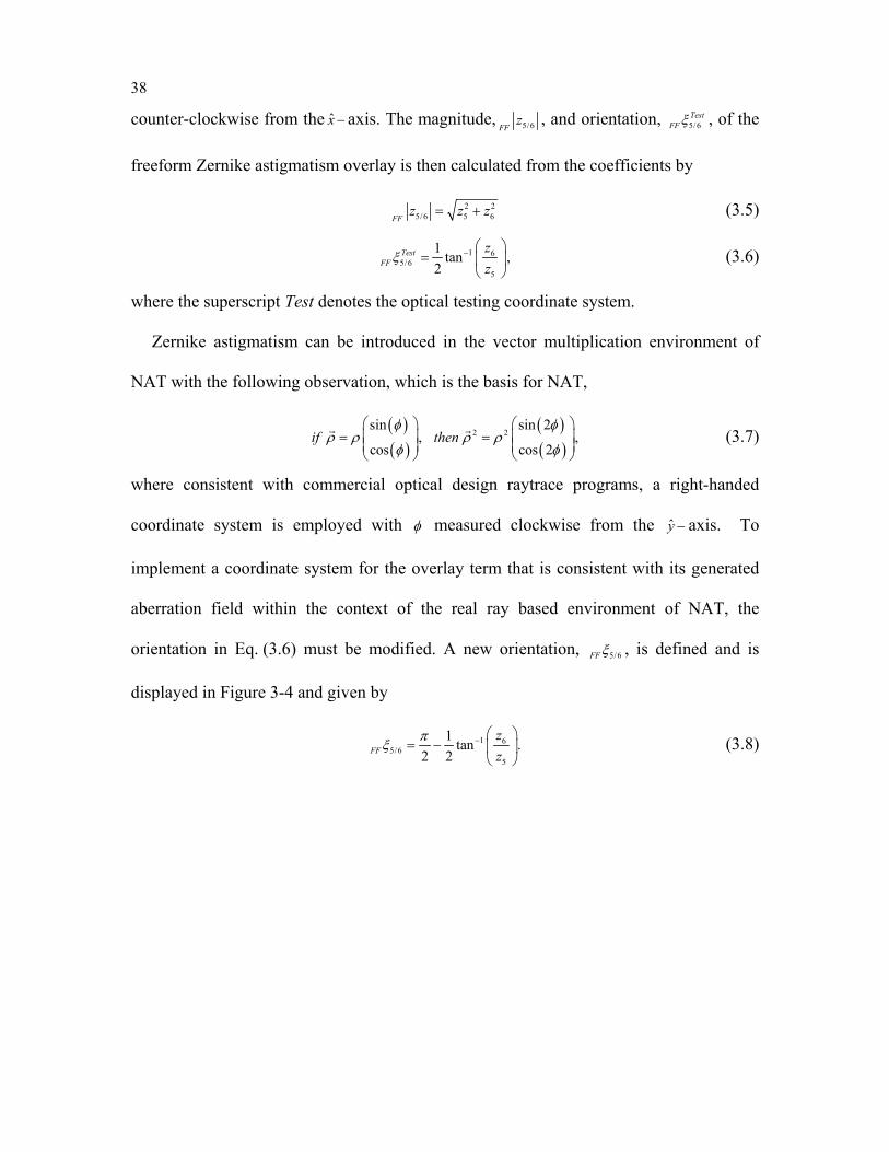
38
counter-clockwise from the x − axis. The magnitude, 5/6FFz , and orientation, 5/6
TestFFξ , of the
freeform Zernike astigmatism overlay is then calculated from the coefficients by
2 25/6 5 6FF
z z z= + (3.5)
1 65/6
5
1 tan ,2
TestFF
zz
ξ − =
(3.6)
where the superscript Test denotes the optical testing coordinate system.
Zernike astigmatism can be introduced in the vector multiplication environment of
NAT with the following observation, which is the basis for NAT,
( )( )
( )( )
2 2sin sin 2
, ,cos cos 2
if thenφ φ
ρ ρ ρ ρφ φ
= =
(3.7)
where consistent with commercial optical design raytrace programs, a right-handed
coordinate system is employed with φ measured clockwise from the y − axis. To
implement a coordinate system for the overlay term that is consistent with its generated
aberration field within the context of the real ray based environment of NAT, the
orientation in Eq. (3.6) must be modified. A new orientation, 5/6FFξ , is defined and is
displayed in Figure 3-4 and given by
1 65/6
5
1 tan .2 2FF
zz
πξ − = −
(3.8)
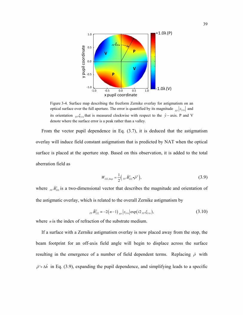
39
x pupil coordinate0.0 0.5 1.0-0.5-1.0
0.0
-0.5
-1.0
0.5
1.0
y pup
il coo
rdin
ate
-
-
-
-
-
0
0
1
1
2
2
+1.0λ (P)
-1.0λ (V)
V
PV
P
5/6FFξ
Figure 3-4. Surface map describing the freeform Zernike overlay for astigmatism on an optical surface over the full aperture. The error is quantified by its magnitude 5/6FF
z and
its orientation 5/6FFξ that is measured clockwise with respect to the y − axis. P and V denote where the surface error is a peak rather than a valley.
From the vector pupil dependence in Eq. (3.7), it is deduced that the astigmatism
overlay will induce field constant astigmatism that is predicted by NAT when the optical
surface is placed at the aperture stop. Based on this observation, it is added to the total
aberration field as
( )2 2222, 222
1 ,2Stop FFW B ρ=
(3.9)
where 2222FF B
is a two-dimensional vector that describes the magnitude and orientation of
the astigmatic overlay, which is related to the overall Zernike astigmatism by
( ) ( )2222 5/6 5/62 1 exp 2 ,FF FFFF
B n z i ξ≡ − −
(3.10)
where n is the index of refraction of the substrate medium.
If a surface with a Zernike astigmatism overlay is now placed away from the stop, the
beam footprint for an off-axis field angle will begin to displace across the surface
resulting in the emergence of a number of field dependent terms. Replacing ρ with
' hρ + ∆
in Eq. (3.9), expanding the pupil dependence, and simplifying leads to a specific
40
set of additive terms for the wavefront expansion when a surface is located away from the
stop,
( )2
2222, 222
2 2 2 2 2222 222 222
1 '21 2 ,2
Not Stop FF
FF FF FF
W B h
B B h B h
ρ
ρ ρ
= + ∆
= + ∆ + ∆
(3.11)
where, as in Section 3.1, the primes on the pupil coordinate have been dropped from the
final expression.
To map the impact of these additive terms on the overall field dependent wave
aberration expansion of an optical system, the pupil dependence needs to be converted
into existing aberration types. To this end, an additional vector operation, introduced
in [20], is used,
* ,A BC AB C=
(3.12)
where *B
is a conjugate vector with the standard properties of a conjugate variable in the
mathematics of complex numbers
( )* ˆ ˆexp .x yB B i B x B yβ= − = − +
(3.13)
By applying the vector identity of Eq. (3.12), Eq. (3.11) takes the form
2 2 2 * 2 2222, 222 222 222
1 2 .2Not Stop FF FF FFW B B h B hρ ρ = + ∆ + ∆
(3.14)
In Eq. (3.14) two additional field dependent aberration terms are generated in addition to
the anticipated field constant astigmatism term. The second and third terms, however, are
a tilt and piston that do not affect the image quality but affect the mapping and phase.
Here we are focusing on the image quality; therefore, these terms will not be directly
addressed for this or any subsequent Zernike overlay terms. In this case, the only image
degrading aberration is field constant astigmatism that is independent of where the
Zernike astigmatism overlay is located with respect to the stop. A magnitude and
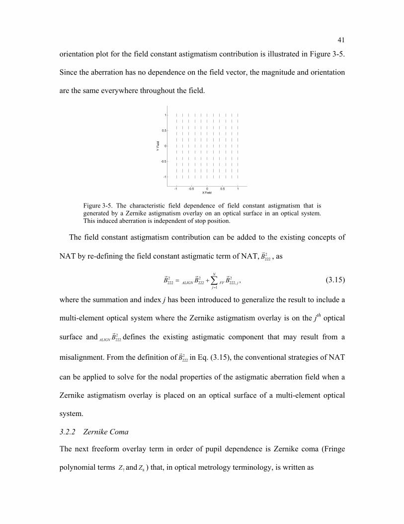
41
orientation plot for the field constant astigmatism contribution is illustrated in Figure 3-5.
Since the aberration has no dependence on the field vector, the magnitude and orientation
are the same everywhere throughout the field.
-1 -0.5 0 0.5 1
-1
-0.5
0
0.5
1
X Field
Y F
ield
Figure 3-5. The characteristic field dependence of field constant astigmatism that is generated by a Zernike astigmatism overlay on an optical surface in an optical system. This induced aberration is independent of stop position.
The field constant astigmatism contribution can be added to the existing concepts of
NAT by re-defining the field constant astigmatic term of NAT, 2222B
, as
2 2 2222 222 222,
1,
N
ALIGN FF jj
B B B=
= +∑
(3.15)
where the summation and index j has been introduced to generalize the result to include a
multi-element optical system where the Zernike astigmatism overlay is on the jth optical
surface and 2222ALIGN B
defines the existing astigmatic component that may result from a
misalignment. From the definition of 2222B
in Eq. (3.15), the conventional strategies of NAT
can be applied to solve for the nodal properties of the astigmatic aberration field when a
Zernike astigmatism overlay is placed on an optical surface of a multi-element optical
system.
3.2.2 Zernike Coma
The next freeform overlay term in order of pupil dependence is Zernike coma (Fringe
polynomial terms 7Z and 8Z ) that, in optical metrology terminology, is written as
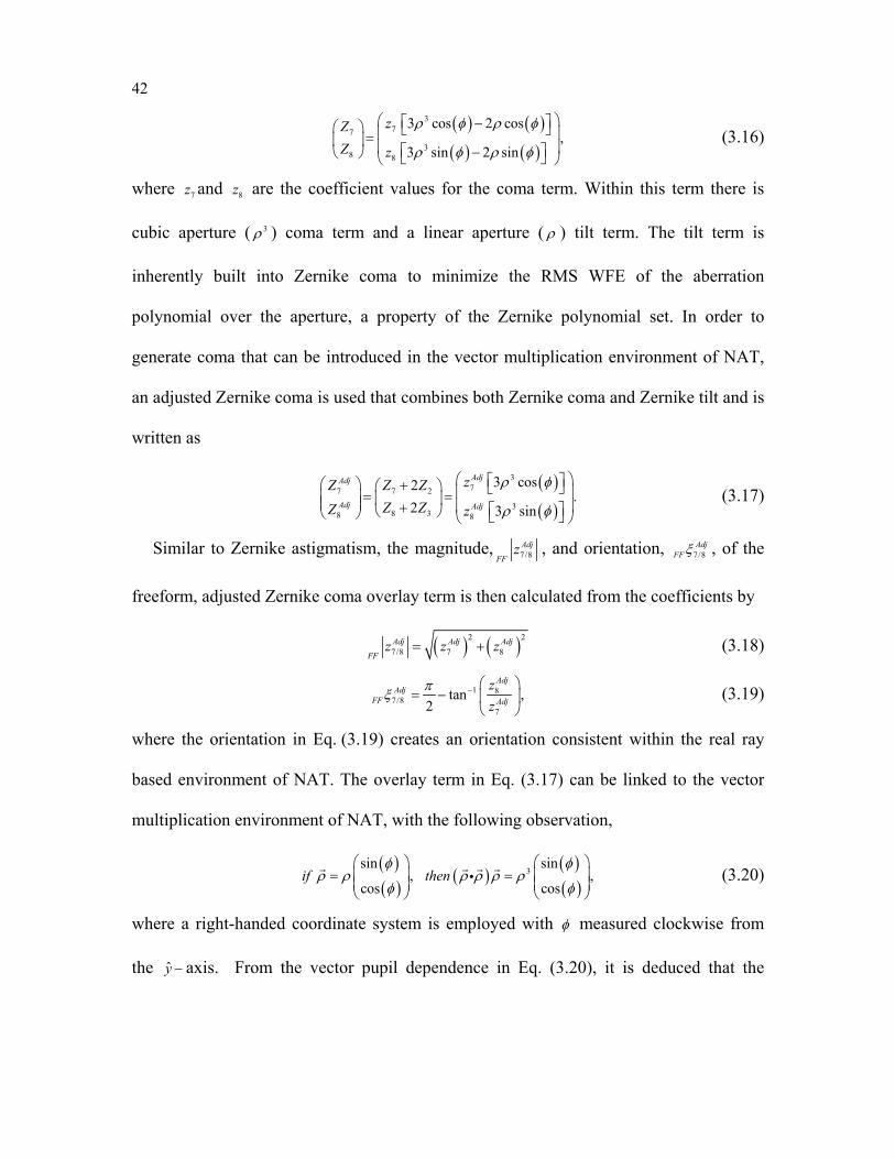
42
( ) ( )( ) ( )
377
38 8
3 cos 2 cos,
3 sin 2 sin
zZZ z
ρ φ ρ φ
ρ φ ρ φ
− = − (3.16)
where 7z and 8z are the coefficient values for the coma term. Within this term there is
cubic aperture ( 3ρ ) coma term and a linear aperture ( ρ ) tilt term. The tilt term is
inherently built into Zernike coma to minimize the RMS WFE of the aberration
polynomial over the aperture, a property of the Zernike polynomial set. In order to
generate coma that can be introduced in the vector multiplication environment of NAT,
an adjusted Zernike coma is used that combines both Zernike coma and Zernike tilt and is
written as
( )( )
377 7 2
38 38 8
3 cos2.
2 3 sin
AdjAdj
Adj Adj
zZ Z ZZ ZZ z
ρ φ
ρ φ
+ = = + (3.17)
Similar to Zernike astigmatism, the magnitude, 7/8Adj
FFz , and orientation, 7/8
AdjFFξ , of the
freeform, adjusted Zernike coma overlay term is then calculated from the coefficients by
( ) ( )2 2
7/8 7 8Adj Adj Adj
FFz z z= + (3.18)
1 87/8
7
tan ,2
AdjAdj
FF Adj
zz
πξ − = −
(3.19)
where the orientation in Eq. (3.19) creates an orientation consistent within the real ray
based environment of NAT. The overlay term in Eq. (3.17) can be linked to the vector
multiplication environment of NAT, with the following observation,
( )( )
( )( )( )
3sin sin
, ,cos cos
if thenφ φ
ρ ρ ρ ρ ρ ρφ φ
= =
(3.20)
where a right-handed coordinate system is employed with φ measured clockwise from
the y − axis. From the vector pupil dependence in Eq. (3.20), it is deduced that the
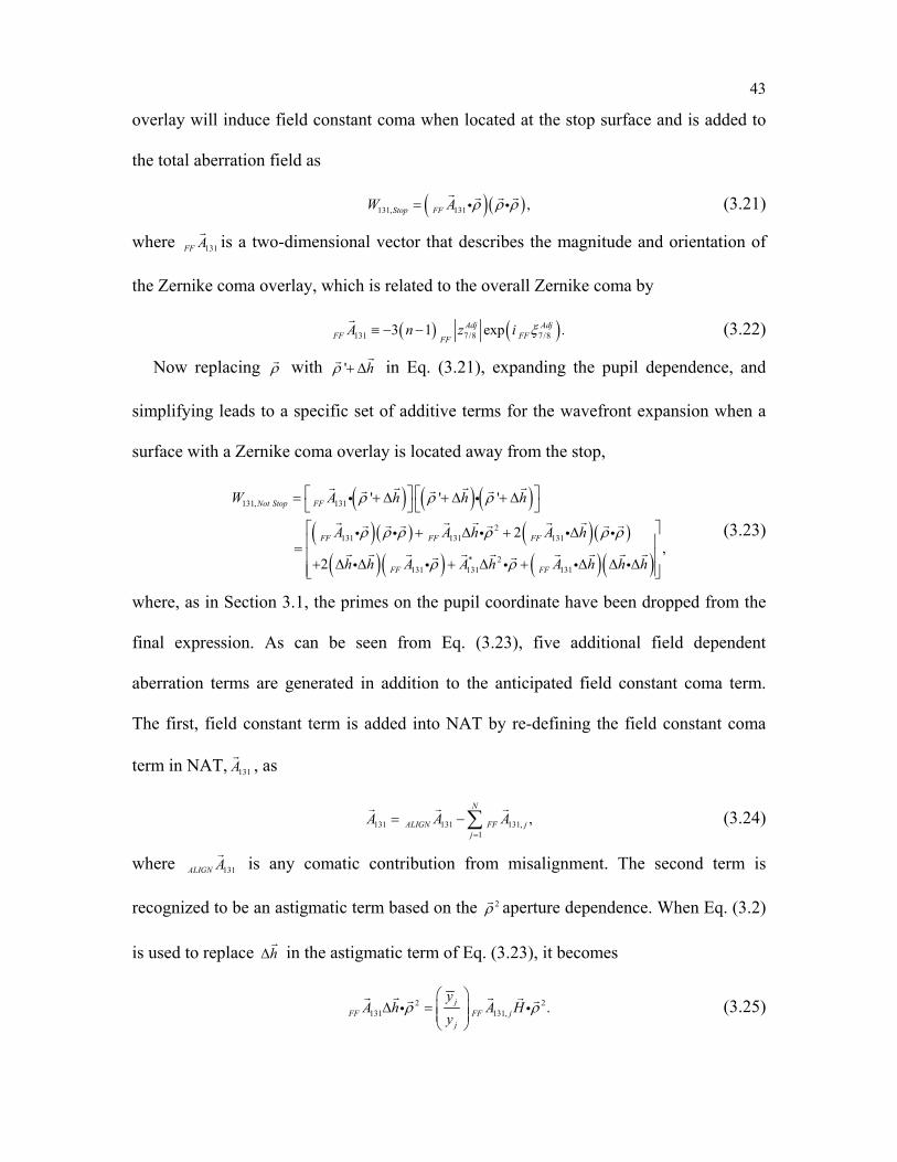
43
overlay will induce field constant coma when located at the stop surface and is added to
the total aberration field as
( )( )131, 131 ,Stop FFW A ρ ρ ρ=
(3.21)
where 131FF A
is a two-dimensional vector that describes the magnitude and orientation of
the Zernike coma overlay, which is related to the overall Zernike coma by
( ) ( )131 7/8 7/83 1 exp .Adj AdjFF FFFF
A n z i ξ≡ − −
(3.22)
Now replacing ρ with ' hρ + ∆
in Eq. (3.21), expanding the pupil dependence, and
simplifying leads to a specific set of additive terms for the wavefront expansion when a
surface with a Zernike coma overlay is located away from the stop,
( ) ( ) ( )( )( ) ( )( )
( )( ) ( )( )
131, 131
2131 131 131
* 2131 131 131
' ' '
2,
2
Not Stop FF
FF FF FF
FF FF
W A h h h
A A h A h
h h A A h A h h h
ρ ρ ρ
ρ ρ ρ ρ ρ ρ
ρ ρ
= + ∆ + ∆ + ∆ + ∆ + ∆ = + ∆ ∆ + ∆ + ∆ ∆ ∆
(3.23)
where, as in Section 3.1, the primes on the pupil coordinate have been dropped from the
final expression. As can be seen from Eq. (3.23), five additional field dependent
aberration terms are generated in addition to the anticipated field constant coma term.
The first, field constant term is added into NAT by re-defining the field constant coma
term in NAT, 131A
, as
131 131 131,1
,N
ALIGN FF jj
A A A=
= −∑
(3.24)
where 131ALIGN A
is any comatic contribution from misalignment. The second term is
recognized to be an astigmatic term based on the 2ρ aperture dependence. When Eq. (3.2)
is used to replace h∆
in the astigmatic term of Eq. (3.23), it becomes
2 2131 131, .j
FF FF jj
yA h A H
yρ ρ
∆ =
(3.25)
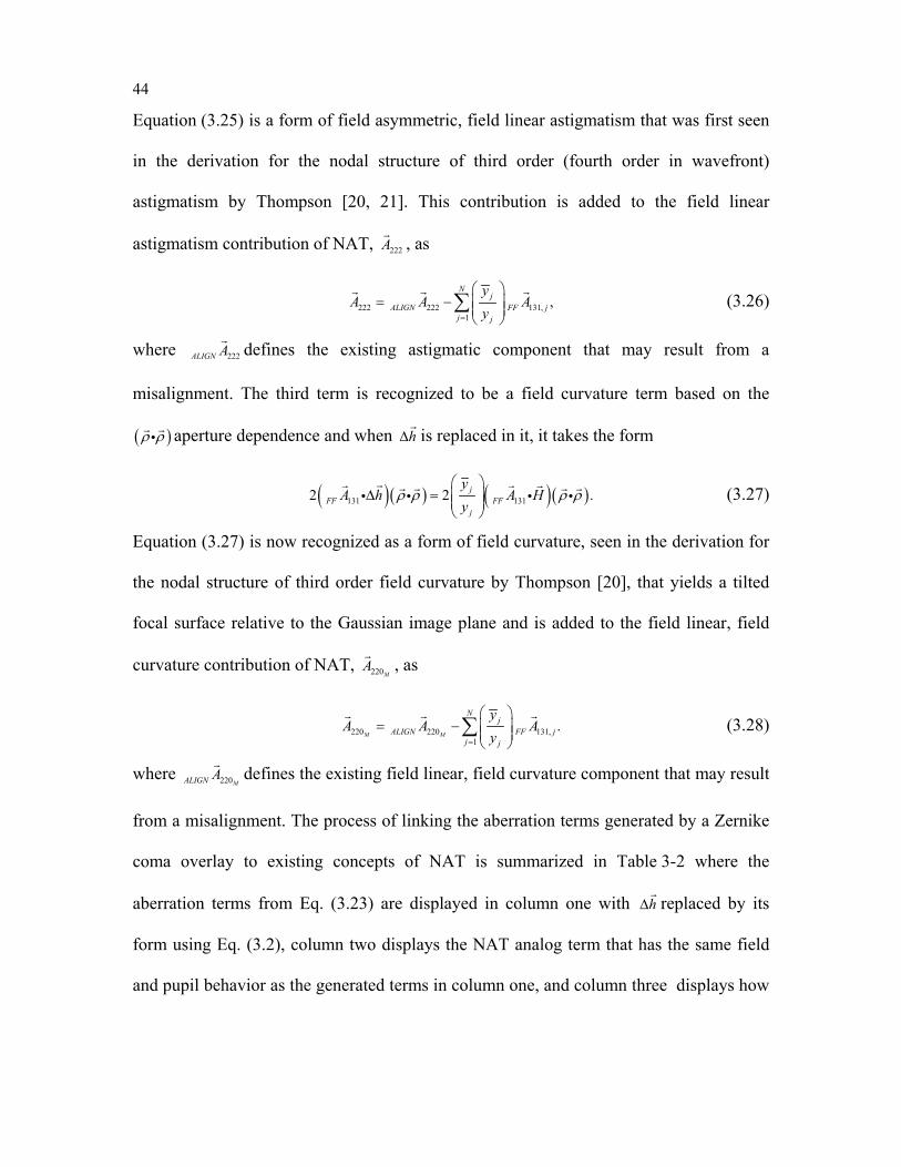
44
Equation (3.25) is a form of field asymmetric, field linear astigmatism that was first seen
in the derivation for the nodal structure of third order (fourth order in wavefront)
astigmatism by Thompson [20, 21]. This contribution is added to the field linear
astigmatism contribution of NAT, 222A
, as
222 222 131,1
,N
jALIGN FF j
j j
yA A A
y=
= −
∑
(3.26)
where 222ALIGN A
defines the existing astigmatic component that may result from a
misalignment. The third term is recognized to be a field curvature term based on the
( )ρ ρ
aperture dependence and when h∆
is replaced in it, it takes the form
( )( ) ( )( )131 1312 2 .jFF FF
j
yA h A H
yρ ρ ρ ρ
∆ =
(3.27)
Equation (3.27) is now recognized as a form of field curvature, seen in the derivation for
the nodal structure of third order field curvature by Thompson [20], that yields a tilted
focal surface relative to the Gaussian image plane and is added to the field linear, field
curvature contribution of NAT, 220MA
, as
220 220 131,1
.M M
Nj
ALIGN FF jj j
yA A A
y=
= −
∑
(3.28)
where 220MALIGN A
defines the existing field linear, field curvature component that may result
from a misalignment. The process of linking the aberration terms generated by a Zernike
coma overlay to existing concepts of NAT is summarized in Table 3-2 where the
aberration terms from Eq. (3.23) are displayed in column one with h∆
replaced by its
form using Eq. (3.2), column two displays the NAT analog term that has the same field
and pupil behavior as the generated terms in column one, and column three displays how
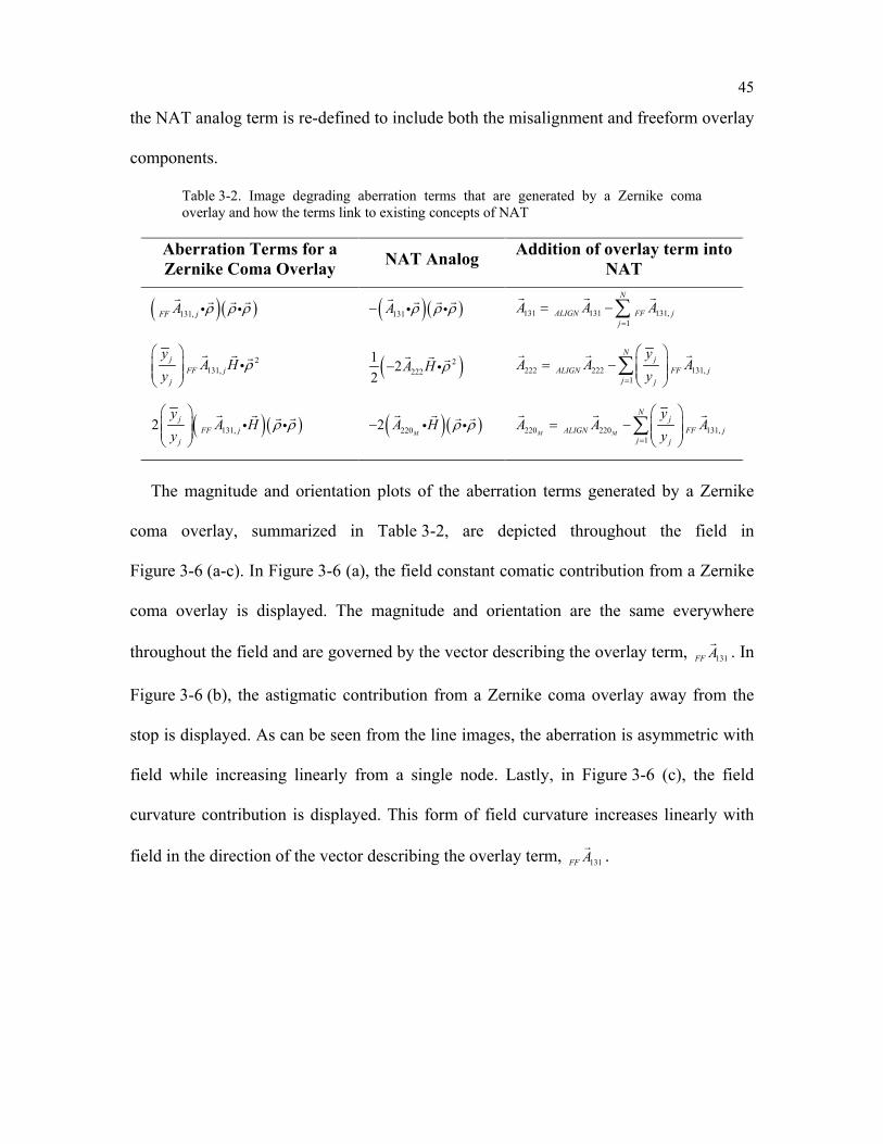
45
the NAT analog term is re-defined to include both the misalignment and freeform overlay
components.
Table 3-2. Image degrading aberration terms that are generated by a Zernike coma overlay and how the terms link to existing concepts of NAT
Aberration Terms for a Zernike Coma Overlay NAT Analog Addition of overlay term into
NAT
( )( )131,FF jA ρ ρ ρ
( )( )131A ρ ρ ρ−
131 131 131,1
N
ALIGN FF jj
A A A=
= −∑
2131,
jFF j
j
yA H
yρ
( )2222
1 22
A H ρ−
222 222 131,1
Nj
ALIGN FF jj j
yA A A
y=
= −
∑
( )( )131,2 jFF j
j
yA H
yρ ρ
( )( )2202M
A H ρ ρ−
220 220 131,1
M M
Nj
ALIGN FF jj j
yA A A
y=
= −
∑
The magnitude and orientation plots of the aberration terms generated by a Zernike
coma overlay, summarized in Table 3-2, are depicted throughout the field in
Figure 3-6 (a-c). In Figure 3-6 (a), the field constant comatic contribution from a Zernike
coma overlay is displayed. The magnitude and orientation are the same everywhere
throughout the field and are governed by the vector describing the overlay term, 131FF A
. In
Figure 3-6 (b), the astigmatic contribution from a Zernike coma overlay away from the
stop is displayed. As can be seen from the line images, the aberration is asymmetric with
field while increasing linearly from a single node. Lastly, in Figure 3-6 (c), the field
curvature contribution is displayed. This form of field curvature increases linearly with
field in the direction of the vector describing the overlay term, 131FF A
.
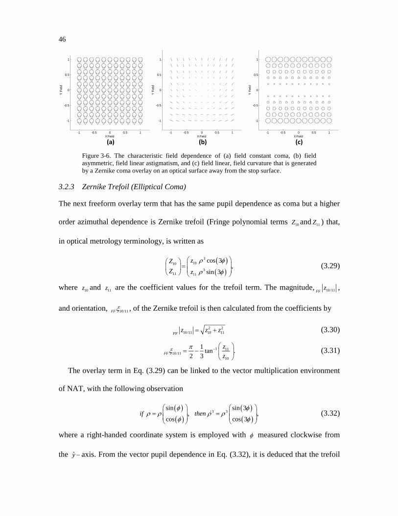
46
-1 -0.5 0 0.5 1
-1
-0.5
0
0.5
1
X Field
Y F
ield
-1 -0.5 0 0.5 1
-1
-0.5
0
0.5
1
X Field
Y F
ield
-1 -0.5 0 0.5 1
-1
-0.5
0
0.5
1
X Field
Y F
ield
(a) (b) (c)
Figure 3-6. The characteristic field dependence of (a) field constant coma, (b) field
asymmetric, field linear astigmatism, and (c) field linear, field curvature that is generated
by a Zernike coma overlay on an optical surface away from the stop surface.
3.2.3 Zernike Trefoil (Elliptical Coma)
The next freeform overlay term that has the same pupil dependence as coma but a higher
order azimuthal dependence is Zernike trefoil (Fringe polynomial terms 10Z and
11Z ) that,
in optical metrology terminology, is written as
3
1010
311 11
cos 3,
sin 3
zZ
Z z
(3.29)
where 10z and
11z are the coefficient values for the trefoil term. The magnitude, 10/11FFz ,
and orientation, 10/11FF , of the Zernike trefoil is then calculated from the coefficients by
2 2
10/11 10 11FFz z z (3.30)
1 11
10/11
10
1tan .
2 3FF
z
z
(3.31)
The overlay term in Eq. (3.29) can be linked to the vector multiplication environment
of NAT, with the following observation
3 3
sin sin 3, ,
cos cos 3if then
(3.32)
where a right-handed coordinate system is employed with measured clockwise from
the y axis. From the vector pupil dependence in Eq. (3.32), it is deduced that the trefoil
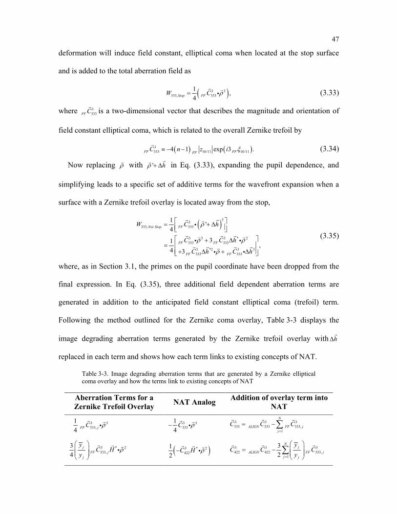
47
deformation will induce field constant, elliptical coma when located at the stop surface
and is added to the total aberration field as
( )3 3333, 333
1 ,4Stop FFW C ρ=
(3.33)
where 3333FF C
is a two-dimensional vector that describes the magnitude and orientation of
field constant elliptical coma, which is related to the overall Zernike trefoil by
( ) ( )3333 10/11 10/114 1 exp 3 .FF FFFF
C n z i ξ≡ − −
(3.34)
Now replacing ρ with ' hρ + ∆
in Eq. (3.33), expanding the pupil dependence, and
simplifying leads to a specific set of additive terms for the wavefront expansion when a
surface with a Zernike trefoil overlay is located away from the stop,
( )3
3333, 333
3 3 3 * 2333 333
3 *2 3 3333 333
1 '4
31 ,4 3
Not Stop FF
FF FF
FF FF
W C h
C C h
C h C h
ρ
ρ ρ
ρ
= + ∆ + ∆
= + ∆ + ∆
(3.35)
where, as in Section 3.1, the primes on the pupil coordinate have been dropped from the
final expression. In Eq. (3.35), three additional field dependent aberration terms are
generated in addition to the anticipated field constant elliptical coma (trefoil) term.
Following the method outlined for the Zernike coma overlay, Table 3-3 displays the
image degrading aberration terms generated by the Zernike trefoil overlay with h∆
replaced in each term and shows how each term links to existing concepts of NAT.
Table 3-3. Image degrading aberration terms that are generated by a Zernike elliptical coma overlay and how the terms link to existing concepts of NAT
Aberration Terms for a Zernike Trefoil Overlay NAT Analog Addition of overlay term into
NAT
3 3333,
14 FF jC ρ
3 3333
14
C ρ−
3 3 3333 333 333,
1
N
ALIGN FF jj
C C C=
= −∑
3 * 2333,
34
jFF j
j
yC H
yρ
( )3 * 2422
12
C H ρ−
3 3 3422 422 333,
1
32
Nj
ALIGN FF jj j
yC C C
y=
= −
∑
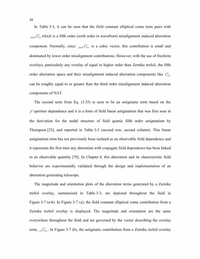
48
In Table 3-3, it can be seen that the field constant elliptical coma term pairs with
3333ALIGN C
which is a fifth order (sixth order in wavefront) misalignment induced aberration
component. Normally, since 3333ALIGN C
is a cubic vector, this contribution is small and
dominated by lower order misalignment contributions. However, with the use of freeform
overlays, particularly any overlay of equal or higher order than Zernike trefoil, the fifth
order aberration space and their misalignment induced aberration components like 3333C
can be roughly equal to or greater than the third order misalignment induced aberration
components of NAT.
The second term from Eq. (3.35) is seen to be an astigmatic term based on the
2ρ aperture dependence and it is a form of field linear astigmatism that was first seen in
the derivation for the nodal structure of field quartic fifth order astigmatism by
Thompson [25], and reported in Table 3-3 (second row, second column). This linear
astigmatism term has not previously been isolated as an observable field dependence and
it represents the first time any aberration with conjugate field dependence has been linked
to an observable quantity [70]. In Chapter 4, this aberration and its characteristic field
behavior are experimentally validated through the design and implementation of an
aberration generating telescope.
The magnitude and orientation plots of the aberration terms generated by a Zernike
trefoil overlay, summarized in Table 3-3, are depicted throughout the field in
Figure 3-7 (a-b). In Figure 3-7 (a), the field constant elliptical coma contribution from a
Zernike trefoil overlay is displayed. The magnitude and orientation are the same
everywhere throughout the field and are governed by the vector describing the overlay
term, 3333FF C
. In Figure 3-7 (b), the astigmatic contribution from a Zernike trefoil overlay
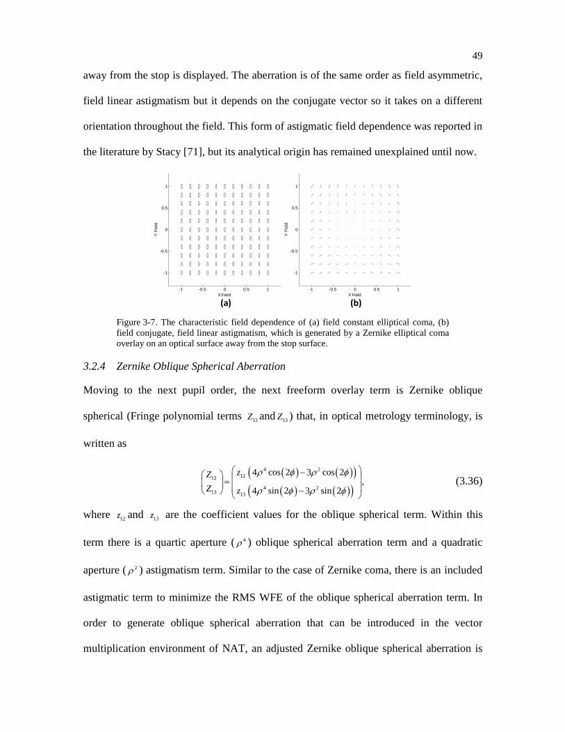
49
away from the stop is displayed. The aberration is of the same order as field asymmetric,
field linear astigmatism but it depends on the conjugate vector so it takes on a different
orientation throughout the field. This form of astigmatic field dependence was reported in
the literature by Stacy [71], but its analytical origin has remained unexplained until now.
-1 -0.5 0 0.5 1
-1
-0.5
0
0.5
1
X Field
Y F
ield
-1 -0.5 0 0.5 1
-1
-0.5
0
0.5
1
X Field
Y F
ield
(a) (b)
Figure 3-7. The characteristic field dependence of (a) field constant elliptical coma, (b)
field conjugate, field linear astigmatism, which is generated by a Zernike elliptical coma
overlay on an optical surface away from the stop surface.
3.2.4 Zernike Oblique Spherical Aberration
Moving to the next pupil order, the next freeform overlay term is Zernike oblique
spherical (Fringe polynomial terms 12Z and
13Z ) that, in optical metrology terminology, is
written as
4 2
1212
4 213 13
4 cos 2 3 cos 2,
4 sin 2 3 sin 2
zZ
Z z
(3.36)
where 12z and
13z are the coefficient values for the oblique spherical term. Within this
term there is a quartic aperture ( 4 ) oblique spherical aberration term and a quadratic
aperture ( 2 ) astigmatism term. Similar to the case of Zernike coma, there is an included
astigmatic term to minimize the RMS WFE of the oblique spherical aberration term. In
order to generate oblique spherical aberration that can be introduced in the vector
multiplication environment of NAT, an adjusted Zernike oblique spherical aberration is

50
used that combines both Zernike oblique spherical aberration and Zernike astigmatism
and is written as
( )( )
41212 512
412 613 13
4 cos 23.
3 4 sin 2
AdjAdj
Adj Adj
zZ ZZZ ZZ z
ρ φ
ρ φ
+ = = + (3.37)
The magnitude, 12/13Adj
FFz , and orientation, 12/13
AdjFFξ , of the freeform, adjusted Zernike oblique
spherical aberration overlay term is then calculated from the coefficients by
( ) ( )2 2
12/13 12 13Adj Adj Adj
FFz z z= + (3.38)
1 1312/13
12
tan .2
AdjAdj
FF Adj
zz
πξ − = −
(3.39)
The overlay term in Eq. (3.37) can be linked to the vector multiplication environment of
NAT, with the following observation
( )( )
( )( )( )
2 4sin sin 2
, ,cos cos 2
if thenφ φ
ρ ρ ρ ρ ρ ρφ φ
= =
(3.40)
where a right-handed coordinate system is employed with φ measured clockwise from
the y − axis. From the vector pupil dependence in Eq.(3.40), it is deduced that the oblique
spherical overlay will induce field constant, oblique spherical aberration when located at
the stop surface and is added to the total aberration field as
( )( )2 2242, 242
1 ,2Stop FFW B ρ ρ ρ=
(3.41)
where 2242FF B
is a two-dimensional vector that describes the magnitude and orientation of
field constant oblique spherical aberration, which relates to adjusted Zernike oblique
spherical aberration by
( ) ( )2242 12/13 12/138 1 exp 2 .Adj Adj
FF FFFFB n z i ξ≡ − −
(3.42)
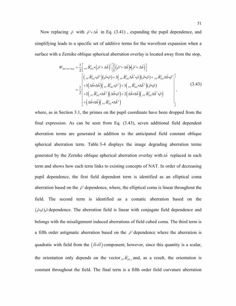
51
Now replacing ρ with ' hρ + ∆
in Eq. (3.41) , expanding the pupil dependence, and
simplifying leads to a specific set of additive terms for the wavefront expansion when a
surface with a Zernike oblique spherical aberration overlay is located away from the stop,
( ) ( ) ( )( )( ) ( )( )
( )( ) ( )( )
( )( ) ( )
22
242, 242
2 2 2 * 2 3242 242 242
2 2 2 2242 242
2 2 2 *242 242
1 ' ' '2
3
3 312 2 2
Not Stop FF
FF FF FF
FF FF
FF FF
W B h h h
B B h B h
h h B B h
B h h h h B h
ρ ρ ρ
ρ ρ ρ ρ ρ ρ ρ
ρ ρ ρ
ρ
= + ∆ + ∆ + ∆
+ ∆ + ∆
+ ∆ ∆ + ∆=
+ ∆ ∆ + ∆ ∆ ∆
( )( )( )2 2
242
,
FFh h B h
ρ
+ ∆ ∆ ∆
(3.43)
where, as in Section 3.1, the primes on the pupil coordinate have been dropped from the
final expression. As can be seen from Eq. (3.43), seven additional field dependent
aberration terms are generated in addition to the anticipated field constant oblique
spherical aberration term. Table 3-4 displays the image degrading aberration terms
generated by the Zernike oblique spherical aberration overlay with h∆
replaced in each
term and shows how each term links to existing concepts of NAT. In order of decreasing
pupil dependence, the first field dependent term is identified as an elliptical coma
aberration based on the 3ρ dependence, where, the elliptical coma is linear throughout the
field. The second term is identified as a comatic aberration based on the
( )ρ ρ ρ
dependence. The aberration field is linear with conjugate field dependence and
belongs with the misalignment induced aberrations of field cubed coma. The third term is
a fifth order astigmatic aberration based on the 2ρ dependence where the aberration is
quadratic with field from the ( )H H
component; however, since this quantity is a scalar,
the orientation only depends on the vector 2242,FF jB
and, as a result, the orientation is
constant throughout the field. The final term is a fifth order field curvature aberration
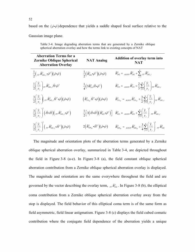
52
based on the ( )ρ ρ
dependence that yields a saddle shaped focal surface relative to the
Gaussian image plane.
Table 3-4. Image degrading aberration terms that are generated by a Zernike oblique spherical aberration overlay and how the terms link to existing concepts of NAT
Aberration Terms for a Zernike Oblique Spherical
Aberration Overlay NAT Analog Addition of overlay term into
NAT
( )( )2 2242,
12 FF jB ρ ρ ρ
( )( )2 2242
12
B ρ ρ ρ
2 2 2242 242 242,
1
N
ALIGN FF jj
B B B=
= +∑
2 3242,
12
jFF j
j
yB H
yρ
( )2 3333
1 34
B H ρ
2 2 2333 333 242,
1
23
Nj
ALIGN FF jj j
yB B B
y=
= +
∑
( )( )2 *242,
32
jFF j
j
yB H
yρ ρ ρ
( )( )2 *331M
B H ρ ρ ρ
2 2 2331 331 242,
1
32M M
Nj
ALIGN FF jj j
yB B B
y=
= +
∑
( )( )2
2 2242,
32
jFF j
j
yH H B
yρ
( )( )2 2422
1 32
H H B ρ
2
2 2 2422 422 242,
1
Nj
ALIGN FF jj j
yB B B
y=
= +
∑
( )( )2
2 2242,
32
jFF j
j
yB H
yρ ρ
( )( )2 24202
MB H ρ ρ
2
2 2 2420 420 242
1
34M M
Nj
ALIGN FFj j
yB B B
y=
= +
∑
The magnitude and orientation plots of the aberration terms generated by a Zernike
oblique spherical aberration overlay, summarized in Table 3-4, are depicted throughout
the field in Figure 3-8 (a-e). In Figure 3-8 (a), the field constant oblique spherical
aberration contribution from a Zernike oblique spherical aberration overlay is displayed.
The magnitude and orientation are the same everywhere throughout the field and are
governed by the vector describing the overlay term, 2242FF B
. In Figure 3-8 (b), the elliptical
coma contribution from a Zernike oblique spherical aberration overlay away from the
stop is displayed. The field behavior of this elliptical coma term is of the same form as
field asymmetric, field linear astigmatism. Figure 3-8 (c) displays the field cubed comatic
contribution where the conjugate field dependence of the aberration yields a unique
53
orientation when compared to conventional third order field linear coma. The fifth order
astigmatic contribution, Figure 3-8 (d), exhibits a field constant orientation while the
magnitude of the aberration varies quadratically with the field vector. Lastly,
Figure 3-8 (e), displays a fifth order field curvature contribution that equates to a saddle
shaped focal plane as the aberration curves up in one direction and down in the other.
-1 -0.5 0 0.5 1
-1
-0.5
0
0.5
1
X Field
Y F
ield
-1 -0.5 0 0.5 1
-1
-0.5
0
0.5
1
X Field
Y F
ield
-1 -0.5 0 0.5 1
-1
-0.5
0
0.5
1
X Field
Y F
ield
-1 -0.5 0 0.5 1
-1
-0.5
0
0.5
1
X Field
Y F
ield
-1 -0.5 0 0.5 1
-1
-0.5
0
0.5
1
X Field
Y F
ield
(a) (b) (c)
(d) (e)
Figure 3-8. The characteristic field dependence of (a) field constant oblique spherical
aberration, (b) field asymmetric, field linear trefoil, (c) field conjugate, field linear coma,
(d) field constant, field quadratic astigmatism, and (e) field quadratic, field curvature that
is generated by a Zernike oblique spherical aberration overlay on an optical surface away
from the stop surface.
3.2.5 Zernike Fifth Order Aperture Coma
The next pupil order and last freeform overlay term is Zernike fifth order aperture coma
(Fringe polynomial terms 14Z and
15Z ) that, in optical metrology terminology, is written as
5 3
1414
5 315 15
10 cos 12 cos 3 cos,
10 sin 12 sin 3 sin
zZ
Z z
(3.44)
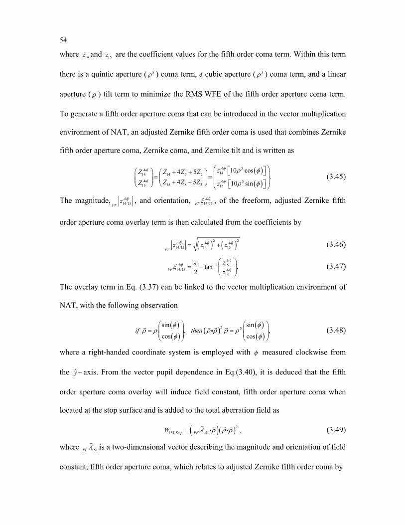
54
where 14z and 15z are the coefficient values for the fifth order coma term. Within this term
there is a quintic aperture ( 5ρ ) coma term, a cubic aperture ( 3ρ ) coma term, and a linear
aperture ( ρ ) tilt term to minimize the RMS WFE of the fifth order aperture coma term.
To generate a fifth order aperture coma that can be introduced in the vector multiplication
environment of NAT, an adjusted Zernike fifth order coma is used that combines Zernike
fifth order aperture coma, Zernike coma, and Zernike tilt and is written as
( )( )
51414 7 214
515 8 315 15
10 cos4 5.
4 5 10 sin
AdjAdj
Adj Adj
zZ Z ZZZ Z ZZ z
ρ φ
ρ φ
+ + = = + + (3.45)
The magnitude, 14/15Adj
FFz , and orientation, 14/15
AdjFFξ , of the freeform, adjusted Zernike fifth
order aperture coma overlay term is then calculated from the coefficients by
( ) ( )2 2
14/15 14 15Adj Adj Adj
FFz z z= + (3.46)
1 1514/15
14
tan .2
AdjAdj
FF Adj
zz
πξ − = −
(3.47)
The overlay term in Eq. (3.37) can be linked to the vector multiplication environment of
NAT, with the following observation
( )( )
( )( )( )
2 5sin sin
, ,cos cos
if thenφ φ
ρ ρ ρ ρ ρ ρφ φ
= =
(3.48)
where a right-handed coordinate system is employed with φ measured clockwise from
the y − axis. From the vector pupil dependence in Eq.(3.40), it is deduced that the fifth
order aperture coma overlay will induce field constant, fifth order aperture coma when
located at the stop surface and is added to the total aberration field as
( )( )2151, 151 ,Stop FFW A ρ ρ ρ=
(3.49)
where 151FF A
is a two-dimensional vector describing the magnitude and orientation of field
constant, fifth order aperture coma, which relates to adjusted Zernike fifth order coma by
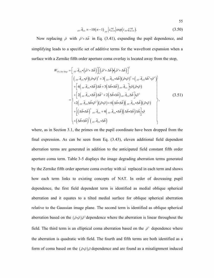
55
( ) ( )151 14/15 14/1510 1 exp .Adj AdjFF FFFF
A n z i ξ≡ − −
(3.50)
Now replacing ρ with ' hρ + ∆
in Eq. (3.41), expanding the pupil dependence, and
simplifying leads to a specific set of additive terms for the wavefront expansion when a
surface with a Zernike fifth order aperture coma overlay is located away from the stop,
( ) ( ) ( )( )( ) ( )( ) ( )
( ) ( ) ( )
( ) ( )
2
151, 151
2 2 2 3151 151 151
151 151
2 2151 151
15
' ' '
3
6 3
2 2
2
Not Stop FF
FF FF FF
FF FF
FF FF
FF
W A h h h
A A h A h
A h h h h A
A h h h h A h
A
ρ ρ ρ
ρ ρ ρ ρ ρ ρ
ρ ρ ρ
ρ
= + ∆ + ∆ + ∆
+ ∆ + ∆
+ ∆ ∆ + ∆ ∆ + ∆ ∆ + ∆ ∆ ∆
=+
( )( ) ( )( )( )
( ) ( )( )( ) ( )
21 151
2
151 151
2
151
,6
4
FF
FF FF
FF
h h h A h
h h A A h h h h
h h A h
ρ ρ ρ ρ ρ
ρ
∆ + ∆ ∆ ∆
+ ∆ ∆ + ∆ ∆ ∆ ∆ + ∆ ∆ ∆
(3.51)
where, as in Section 3.1, the primes on the pupil coordinate have been dropped from the
final expression. As can be seen from Eq. (3.43), eleven additional field dependent
aberration terms are generated in addition to the anticipated field constant fifth order
aperture coma term. Table 3-5 displays the image degrading aberration terms generated
by the Zernike fifth order aperture coma overlay with h∆
replaced in each term and shows
how each term links to existing concepts of NAT. In order of decreasing pupil
dependence, the first field dependent term is identified as medial oblique spherical
aberration and it equates to a tilted medial surface for oblique spherical aberration
relative to the Gaussian image plane. The second term is identified as oblique spherical
aberration based on the ( ) 2ρ ρ ρ
dependence where the aberration is linear throughout the
field. The third term is an elliptical coma aberration based on the 3ρ dependence where
the aberration is quadratic with field. The fourth and fifth terms are both identified as a
form of coma based on the ( )ρ ρ ρ
dependence and are found as a misalignment induced
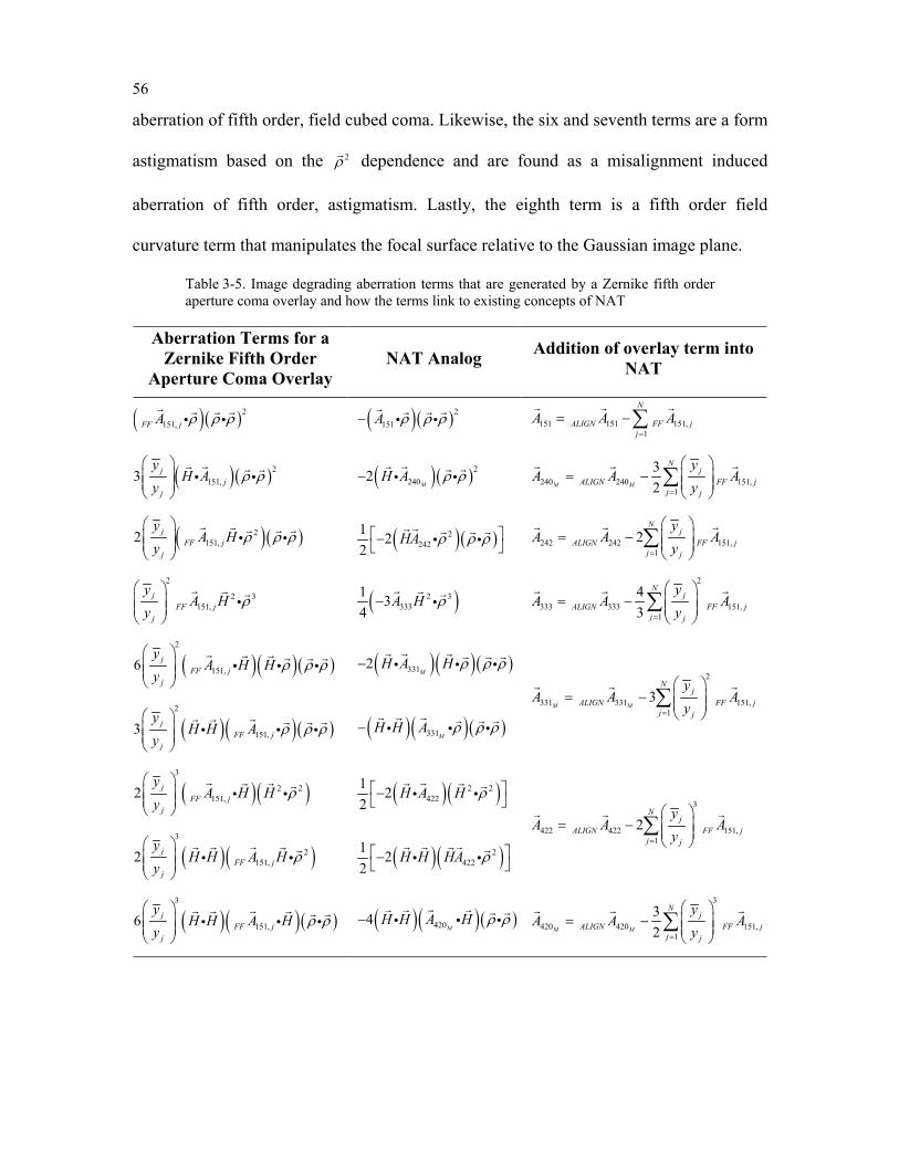
56
aberration of fifth order, field cubed coma. Likewise, the six and seventh terms are a form
astigmatism based on the 2ρ dependence and are found as a misalignment induced
aberration of fifth order, astigmatism. Lastly, the eighth term is a fifth order field
curvature term that manipulates the focal surface relative to the Gaussian image plane.
Table 3-5. Image degrading aberration terms that are generated by a Zernike fifth order aperture coma overlay and how the terms link to existing concepts of NAT
Aberration Terms for a Zernike Fifth Order
Aperture Coma Overlay NAT Analog Addition of overlay term into
NAT
( )( )2151,FF jA ρ ρ ρ
( )( )2151A ρ ρ ρ−
151 151 151,1
N
ALIGN FF jj
A A A=
= −∑
( )( )2151,3 j
jj
yH A
yρ ρ
( )( )22402
MH A ρ ρ−
240 240 151,1
32M M
Nj
ALIGN FF jj j
yA A A
y=
= −
∑
( )( )2151,2 j
FF jj
yA H
yρ ρ ρ
( )( )2242
1 22
HA ρ ρ ρ −
242 242 151,1
2N
jALIGN FF j
j j
yA A A
y=
= −
∑
2
2 3151,
jFF j
j
yA H
yρ
( )2 3333
1 34
A H ρ−
2
333 333 151,1
43
Nj
ALIGN FF jj j
yA A A
y=
= −
∑
( )( )( )2
151,6 jFF j
j
yA H H
yρ ρ ρ
( )( )( )3312M
H A H ρ ρ ρ−
2
331 331 151,1
3M M
Nj
ALIGN FF jj j
yA A A
y=
= −
∑
( )( )( )2
151,3 jFF j
j
yH H A
yρ ρ ρ
( )( )( )331MH H A ρ ρ ρ−
( )( )3
2 2151,2 j
FF jj
yA H H
yρ
( )( )2 2422
1 22
H A H ρ −
3
422 422 151,1
2N
jALIGN FF j
j j
yA A A
y=
= −
∑
( )( )3
2151,2 j
FF jj
yH H A H
yρ
( )( )2422
1 22
H H HA ρ −
( )( )( )3
151,6 jFF j
j
yH H A H
yρ ρ
( )( )( )4204M
H H A H ρ ρ−
3
420 420 151,1
32M M
Nj
ALIGN FF jj j
yA A A
y=
= −
∑
57
The magnitude and orientation plots of the aberration terms generated by a Zernike
fifth order aperture coma overlay, summarized in Table 3-5, are depicted throughout the
field in Figure 3-9 (a-g). In Figure 3-9 (a), the field constant fifth order aperture coma
contribution from a Zernike fifth order aperture coma overlay is displayed. The
magnitude and orientation are the same everywhere throughout the field and are governed
by the vector describing the overlay term, 151FF A
. In Figure 3-9 (b), the medial oblique
spherical aberration contribution from a Zernike fifth order aperture coma overlay away
from the stop is displayed. The field behavior of this term resembles that of the field
curvature term generated by a Zernike coma overlay. Figure 3-9 (c) displays the oblique
spherical aberration contribution where the field behavior resembles that of field
asymmetric, field linear astigmatism. The elliptical coma contribution, Figure 3-9 (d), is
field quadratic and depending on the vector describing the overlay term, 151FF A
, the
aberration orientation may appear rotationally symmetric as is depicted in Figure 3-9 (d).
In Figure 3-9 (e), the two field quadratic coma contributions are displayed together
resulting in a net field asymmetric aberration. Similarly, Figure 3-9 (f) displays together
the two field cubed, fifth order astigmatism contributions, resulting in a net aberration
that is field asymmetric. Lastly, Figure 3-9 (g), displays a fifth order field curvature
contribution that equates to a cubic shaped focal plane.
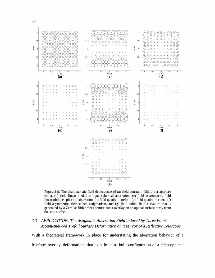
58
-1 -0.5 0 0.5 1
-1
-0.5
0
0.5
1
X Field
Y F
ield
-1 -0.5 0 0.5 1
-1
-0.5
0
0.5
1
X Field
Y F
ield
-1 -0.5 0 0.5 1
-1
-0.5
0
0.5
1
X Field
Y F
ield
-1 -0.5 0 0.5 1
-1
-0.5
0
0.5
1
X Field
Y F
ield
-1 -0.5 0 0.5 1
-1
-0.5
0
0.5
1
X Field
Y F
ield
-1 -0.5 0 0.5 1
-1
-0.5
0
0.5
1
X Field
Y F
ield
-1 -0.5 0 0.5 1
-1
-0.5
0
0.5
1
X Field
Y F
ield
(a) (b) (c)
(d) (e) (f)
(g)
Figure 3-9. The characteristic field dependence of (a) field constant, fifth order aperture
coma, (b) field linear medial oblique spherical aberration, (c) field asymmetric, field
linear oblique spherical aberration, (d) field quadratic trefoil, (e) field quadratic coma, (f)
field asymmetric, field cubed astigmatism, and (g) field cubic, field curvature that is
generated by a Zernike fifth order aperture coma overlay on an optical surface away from
the stop surface.
3.3 APPLICATION: The Astigmatic Aberration Field Induced by Three Point
Mount-Induced Trefoil Surface Deformation on a Mirror of a Reflective Telescope
With a theoretical framework in place for understating the aberration behavior of a
freeform overlay, deformations that exist in an as-built configuration of a telescope can
59
be studied. The deformation of particular interest here is the self weight deflection of an
optic located away from the aperture stop being held at three points, a kinematically
stable condition. An error of this nature is usually measured interferometrically by
measuring the optic in its on-axis, null configuration while in its in-use mounting
configuration; or, the error can be simulated by the use of finite element methods [72]. In
either the measured or simulated case, the deformation is quantified based on the values
of its Fringe Zernike coefficients. The predominant surface error that arises with this
mount configuration is trefoil, in optical testing terminology, Fringe polynomial terms
10Z and 11Z . In Section 3.2, the field aberration influence of a trefoil surface overlay was
described. The next step is to apply these results to various reflective telescope forms to
observe the impact of the mount-induced trefoil deformation from the nominal telescope
configuration.
Depending on the telescope optical configuration, the third order aberrations, i.e.
spherical aberration, coma, and astigmatism, may or may not be corrected. For the case of
a two mirror telescope, the system is corrected for third order spherical aberration and
may be corrected for third order coma depending on the conic distribution of the mirrors.
Whether or not coma is corrected, third order astigmatism remains uncorrected. If a third
mirror is added, the telescope system may also be corrected for third order astigmatism.
In either the two or three mirror case, when the secondary mirror is deformed by a three
point mount, it will generate a field dependent astigmatic contribution, assuming the
secondary mirror is not the stop surface. Under these conditions, the astigmatic response
of the telescope is of interest because it reveals information into the as-built state of the
60
telescope. In the case described above, the astigmatic response, ASTW , of the telescope
takes the nodal form
2 3 * 2222 333,
1 3 ,2 4
SMAST MNTERR SM
SM
yW W H C H
yρ
= +
(3.52)
where the subscript SM signifies that the mount-induced trefoil deformation is on the
secondary mirror surface and depending on whether the telescope is anastigmatic,
222W may or may not be equal to zero.
To emphasize, Eq. (3.52) presents the magnitude and orientation of the astigmatic
Fringe Zernike coefficients (Z5/6) that would be measured if an interferogram was
collected at the field point H
in the FOV of the perturbed telescope. The perturbation, in
this case, is a three point kinematic mount deformation on the secondary mirror,
characterized by 3333,MNTERR SMC
, and is directly related to the measured values of the Fringe
Zernike trefoil (Z10/11) following Eq. (3.34).
To exploit the strength of NAT for developing insight into the relationships between
alignment, fabrication, uncorrected aberration fields, and now mount-induced errors, the
next step is to understand the nodal response of the astigmatism to these deviations from
a nominal design depending on whether the system is corrected for third order
astigmatism.
3.3.1 Astigmatic Reflective Telescope Configuration ( 222 0W ≠ ) in the Presence of a Three Point Mount-Induced Surface Deformation on the Secondary Mirror
In order to determine the possible nodal geometry for the case where residual third order
astigmatism exists, the term inside the brackets of Eq. (3.52) is set equal to zero, as
represented in Eq. (3.53),
61
2 3 *222 333,
1 3 0.2 4
SMMNTERR SM
SM
yW H C H
y
+ =
(3.53)
The first step in solving the vector formulation represented in Eq. (3.53) is to establish
a path for arranging 2H
and *H
in a form that can be solved, ideally using previously
developed techniques. This step is accomplished by multiplying both sides of Eq. (3.53)
by unity in the form of
* *
2 2ˆ ˆ0 1 ,HH H Hi j
H H+ = =
(3.54)
where a vector multiplication relation presented in [20] has been applied. Since Eq. (3.54)
is a unit, vector formulation, it does not affect the magnitude or orientation of either
vector in Eq. (3.53). Multiplying the identity in Eq. (3.54) through Eq. (3.53) yields
3 3 * *222 333,2
1 1 3 0.2 4
SMMNTERR SM
SM
yW H C H H H
yH
+ =
(3.55)
Again, making use of the identity in Eq. (3.54), Eq. (3.55) takes the form
3
3 *222 333,2
1 3 0.2 4
SMMNTERR SM
SM
yHW C HyH
+ =
(3.56)
It can now be seen based on the powers of H
that there is a quadranodal astigmatic
response in the FOV to a mount-induced trefoil deformation on the secondary mirror with
the term in the brackets of Eq. (3.56) exhibiting equilateral trinodal behavior with a
fourth zero located on-axis at 0H =
. In order to find the nodal response, the term inside
the bracket of Eq. (3.56) is rearranged, and set to zero, taking the form
3
3333,2
222
3 0.2
SMMNTERR SM
SM
yH CW yH
+ =
(3.57)
The first term of Eq. (3.57) is substituted with a new reduced field vector 3Π
written in
complex notation as
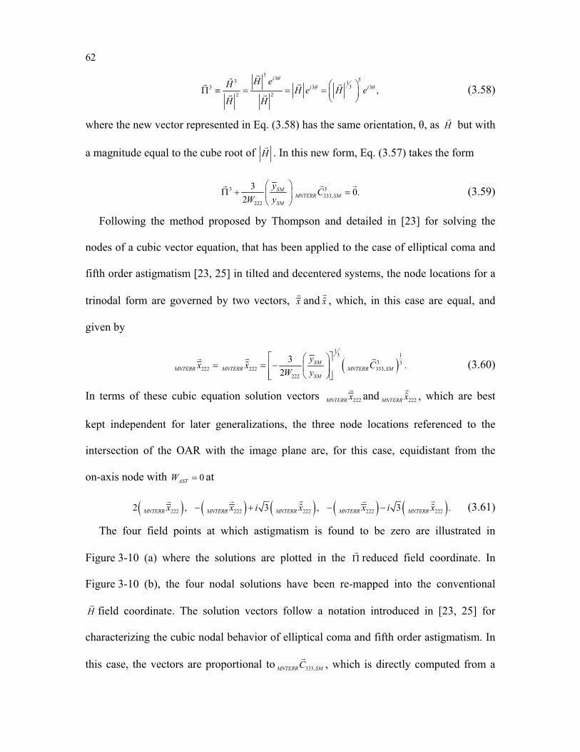
62
3 3 33 1
33 3 32 2 ,
ii i
H eH H e H eH H
θ
θ θ Π ≡ = = =
(3.58)
where the new vector represented in Eq. (3.58) has the same orientation, θ, as H
but with
a magnitude equal to the cube root of H
. In this new form, Eq. (3.57) takes the form
3 3333,
222
3 0.2
SMMNTERR SM
SM
yC
W y
Π + =
(3.59)
Following the method proposed by Thompson and detailed in [23] for solving the
nodes of a cubic vector equation, that has been applied to the case of elliptical coma and
fifth order astigmatism [23, 25] in tilted and decentered systems, the node locations for a
trinodal form are governed by two vectors, x
and x
, which, in this case are equal, and
given by
( )1
3 13 3
222 222 333,222
3 .2
SMMNTERR MNTERR MNTERR SM
SM
yx x C
W y
= = −
(3.60)
In terms of these cubic equation solution vectors 222MNTERR x
and 222MNTERR x
, which are best
kept independent for later generalizations, the three node locations referenced to the
intersection of the OAR with the image plane are, for this case, equidistant from the
on-axis node with 0ASTW = at
( ) ( ) ( ) ( ) ( )222 222 222 222 2222 , 3 , 3 .MNTERR MNTERR MNTERR MNTERR MNTERRx x i x x i x− + − −
(3.61)
The four field points at which astigmatism is found to be zero are illustrated in
Figure 3-10 (a) where the solutions are plotted in the Π
reduced field coordinate. In
Figure 3-10 (b), the four nodal solutions have been re-mapped into the conventional
H
field coordinate. The solution vectors follow a notation introduced in [23, 25] for
characterizing the cubic nodal behavior of elliptical coma and fifth order astigmatism. In
this case, the vectors are proportional to 333,MNTERR SMC
, which is directly computed from a
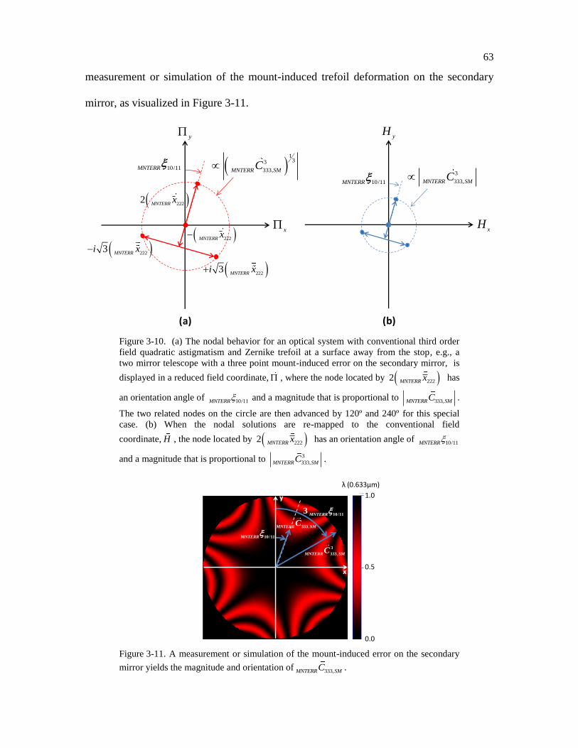
63
measurement or simulation of the mount-induced trefoil deformation on the secondary
mirror, as visualized in Figure 3-11.
x
y
xH
yH
(a) (b)
1
33
333,MNTERR SMC
3
333,MNTERR SMC
10/11MNTERR
10/11MNTERR
2222
MNTERRx
222MNTERRx
2223
MNTERRi x
2223
MNTERRi x
Figure 3-10. (a) The nodal behavior for an optical system with conventional third order
field quadratic astigmatism and Zernike trefoil at a surface away from the stop, e.g., a
two mirror telescope with a three point mount-induced error on the secondary mirror, is
displayed in a reduced field coordinate, , where the node located by 2222 MNTERR x has
an orientation angle of 10/11MNTERR and a magnitude that is proportional to 333,MNTERR SMC .
The two related nodes on the circle are then advanced by 120º and 240º for this special
case. (b) When the nodal solutions are re-mapped to the conventional field
coordinate, H , the node located by 2222 MNTERR x has an orientation angle of 10/11MNTERR
and a magnitude that is proportional to 3
333,MNTERR SMC .
Waves
0.0000
1.0000
0.5000
WAVEFRONT ABERRATION
Cassegrain Ritchey-Chretien
Field = ( 0.000, 0.000) DegreesWavelength = 632.8 nmDefocusing = 0.000000 mm
λ (0.633µm)
10/113
MNTERR
10/11MNTERR
,
3
333MNTERR SMC
,333MNTERR SMC
1.0
0.5
0.0
x
y
2222x
222x
2223i x
2223i x
x
y
(a) (b)
10/11MNTERR
Figure 3-11. A measurement or simulation of the mount-induced error on the secondary
mirror yields the magnitude and orientation of 333,MNTERR SMC .
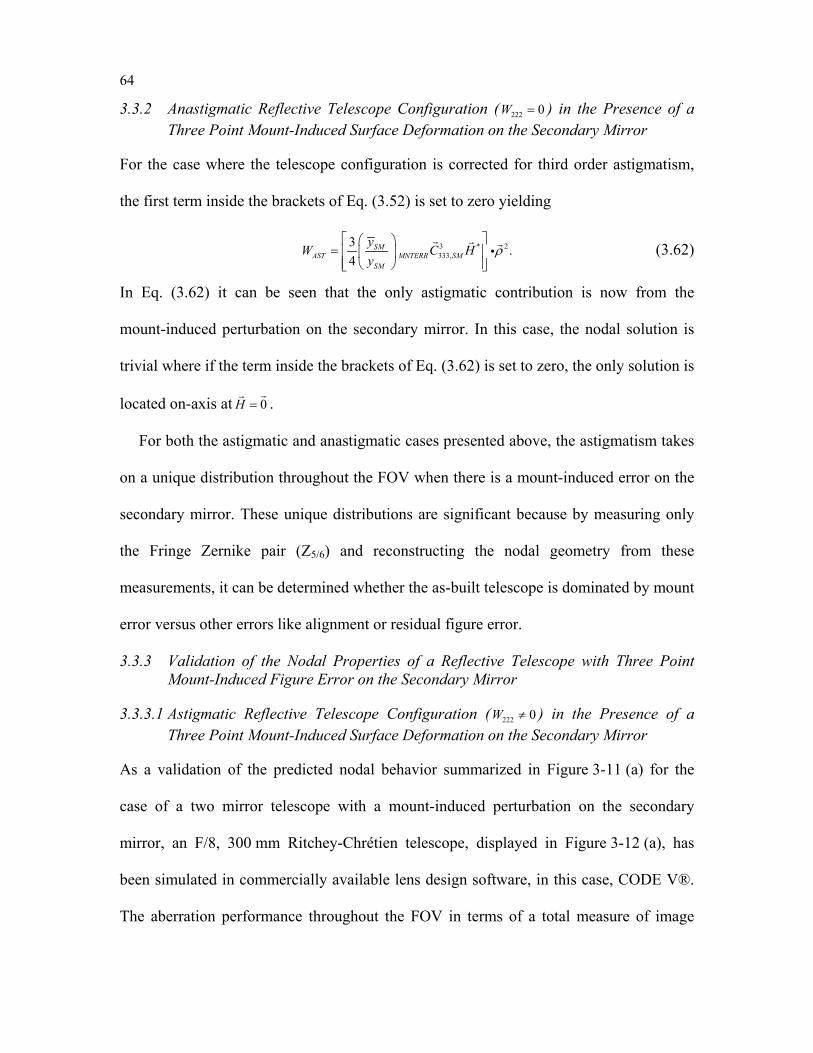
64
3.3.2 Anastigmatic Reflective Telescope Configuration ( 222 0W = ) in the Presence of a Three Point Mount-Induced Surface Deformation on the Secondary Mirror
For the case where the telescope configuration is corrected for third order astigmatism,
the first term inside the brackets of Eq. (3.52) is set to zero yielding
3 * 2333,
3 .4
SMAST MNTERR SM
SM
yW C H
yρ
=
(3.62)
In Eq. (3.62) it can be seen that the only astigmatic contribution is now from the
mount-induced perturbation on the secondary mirror. In this case, the nodal solution is
trivial where if the term inside the brackets of Eq. (3.62) is set to zero, the only solution is
located on-axis at 0H =
.
For both the astigmatic and anastigmatic cases presented above, the astigmatism takes
on a unique distribution throughout the FOV when there is a mount-induced error on the
secondary mirror. These unique distributions are significant because by measuring only
the Fringe Zernike pair (Z5/6) and reconstructing the nodal geometry from these
measurements, it can be determined whether the as-built telescope is dominated by mount
error versus other errors like alignment or residual figure error.
3.3.3 Validation of the Nodal Properties of a Reflective Telescope with Three Point Mount-Induced Figure Error on the Secondary Mirror
3.3.3.1 Astigmatic Reflective Telescope Configuration ( 222 0W ≠ ) in the Presence of a Three Point Mount-Induced Surface Deformation on the Secondary Mirror
As a validation of the predicted nodal behavior summarized in Figure 3-11 (a) for the
case of a two mirror telescope with a mount-induced perturbation on the secondary
mirror, an F/8, 300 mm Ritchey-Chrétien telescope, displayed in Figure 3-12 (a), has
been simulated in commercially available lens design software, in this case, CODE V®.
The aberration performance throughout the FOV in terms of a total measure of image
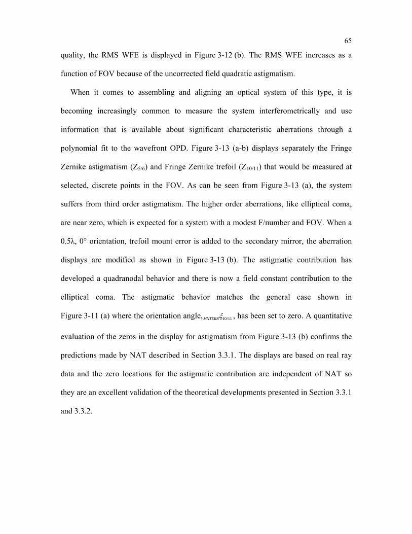
65
quality, the RMS WFE is displayed in Figure 3-12 (b). The RMS WFE increases as a
function of FOV because of the uncorrected field quadratic astigmatism.
When it comes to assembling and aligning an optical system of this type, it is
becoming increasingly common to measure the system interferometrically and use
information that is available about significant characteristic aberrations through a
polynomial fit to the wavefront OPD. Figure 3-13 (a-b) displays separately the Fringe
Zernike astigmatism (Z5/6) and Fringe Zernike trefoil (Z10/11) that would be measured at
selected, discrete points in the FOV. As can be seen from Figure 3-13 (a), the system
suffers from third order astigmatism. The higher order aberrations, like elliptical coma,
are near zero, which is expected for a system with a modest F/number and FOV. When a
0.5λ, 0° orientation, trefoil mount error is added to the secondary mirror, the aberration
displays are modified as shown in Figure 3-13 (b). The astigmatic contribution has
developed a quadranodal behavior and there is now a field constant contribution to the
elliptical coma. The astigmatic behavior matches the general case shown in
Figure 3-11 (a) where the orientation angle, , has been set to zero. A quantitative
evaluation of the zeros in the display for astigmatism from Figure 3-13 (b) confirms the
predictions made by NAT described in Section 3.3.1. The displays are based on real ray
data and the zero locations for the astigmatic contribution are independent of NAT so
they are an excellent validation of the theoretical developments presented in Section 3.3.1
and 3.3.2.
10/11MNTERR
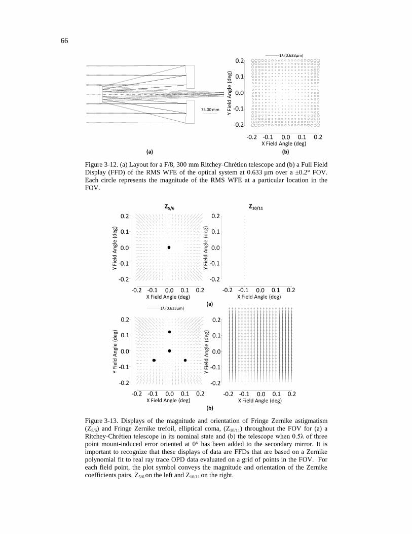
66
16:08:28
telescope_102209
KPT 05-Jun-12
RMS WAVEFRONT ERROR
vs
REAL RAY IMAGE HEIGHT
Minimum = 0.015705
Maximum = 0.20333
Average = 0.082848
Std Dev = 0.043672
1waves ( 632.8 nm)
-10 -5 0 5 10
X Real Ray Image Height - mm
-10
-5
0
5
10
Y Real Ray Image Height - mm
14:24:20
telescope_102209
KPT 13-May-12
FRINGE ZERNIKE PAIR Z5 AND Z6
vs
REAL RAY IMAGE HEIGHT
Minimum = 0.15806e-9
Maximum = 0.44379
Average = 0.16275
Std Dev = 0.10257
1waves ( 632.8 nm)
-10 -5 0 5 10
X Real Ray Image Height - mm
-10
-5
0
5
10
Y Real Ray Image Height - mm
1λ (0.633µm)
(a)
(b)
Y Fi
eld
An
gle
(deg
)
0.2
0.1
0.0
-0.1
-0.2
X Field Angle (deg)-0.2 -0.1 0.0 0.1 0.2
16:02:10
telescope_102209 Scale: 0.33 KPT 05-Jun-12
75.00 MM
16:02:10
telescope_102209 Scale: 0.33 KPT 05-Jun-12
75.00 MM
(b)
75.00 mm
Figure 3-12. (a) Layout for a F/8, 300 mm Ritchey-Chrétien telescope and (b) a Full Field
Display (FFD) of the RMS WFE of the optical system at 0.633 µm over a ±0.2° FOV.
Each circle represents the magnitude of the RMS WFE at a particular location in the
FOV.
14:24:20
telescope_102209
KPT 13-May-12
FRINGE ZERNIKE PAIR Z5 AND Z6
vs
REAL RAY IMAGE HEIGHT
Minimum = 0.15806e-9
Maximum = 0.44379
Average = 0.16275
Std Dev = 0.10257
1waves ( 632.8 nm)
-10 -5 0 5 10
X Real Ray Image Height - mm
-10
-5
0
5
10
Y Real Ray Image Height - mm
14:16:32
telescope_102209
KPT 13-May-12
FRINGE ZERNIKE PAIR Z5 AND Z6
vs
REAL RAY IMAGE HEIGHT
Minimum = 0.3246e-7
Maximum = 0.59586
Average = 0.18471
Std Dev = 0.12847
1waves ( 632.8 nm)
-10 -5 0 5 10
X Real Ray Image Height - mm
-10
-5
0
5
10
Y Real Ray Image Height - mm
14:03:40
telescope_102209
KPT 13-May-12
FRINGE ZERNIKE PAIR Z10 AND Z11
vs
REAL RAY IMAGE HEIGHT
Minimum = 0.28221e-15
Maximum = 0.00014343
Average = 0.36672e-4
Std Dev = 0.31462e-4
1waves ( 632.8 nm)
-10 -5 0 5 10
X Real Ray Image Height - mm
-10
-5
0
5
10
Y Real Ray Image Height - mm
14:11:34
telescope_102209
KPT 13-May-12
FRINGE ZERNIKE PAIR Z10 AND Z11
vs
REAL RAY IMAGE HEIGHT
Minimum = 0.98331
Maximum = 0.98381
Average = 0.98345
Std Dev = 0.98902e-4
1waves ( 632.8 nm)
-10 -5 0 5 10
X Real Ray Image Height - mm
-10
-5
0
5
10
Y Real Ray Image Height - mm
Y Fi
eld
An
gle
(deg
)
0.2
0.1
0.0
-0.1
-0.2
X Field Angle (deg)-0.2 -0.1 0.0 0.1 0.2
Z10/11Z5/6
(a)
(b)
Y Fi
eld
An
gle
(deg
)
0.2
0.1
0.0
-0.1
-0.2
X Field Angle (deg)-0.2 -0.1 0.0 0.1 0.2
Y Fi
eld
An
gle
(deg
)
0.2
0.1
0.0
-0.1
-0.2
X Field Angle (deg)-0.2 -0.1 0.0 0.1 0.2
Y Fi
eld
An
gle
(deg
)
0.2
0.1
0.0
-0.1
-0.2
X Field Angle (deg)-0.2 -0.1 0.0 0.1 0.2
14:24:20
telescope_102209
KPT 13-May-12
FRINGE ZERNIKE PAIR Z5 AND Z6
vs
REAL RAY IMAGE HEIGHT
Minimum = 0.15806e-9
Maximum = 0.44379
Average = 0.16275
Std Dev = 0.10257
1waves ( 632.8 nm)
-10 -5 0 5 10
X Real Ray Image Height - mm
-10
-5
0
5
10
Y Real Ray Image Height - mm
1λ (0.633µm)
Figure 3-13. Displays of the magnitude and orientation of Fringe Zernike astigmatism
(Z5/6) and Fringe Zernike trefoil, elliptical coma, (Z10/11) throughout the FOV for (a) a
Ritchey-Chrétien telescope in its nominal state and (b) the telescope when 0.5λ of three
point mount-induced error oriented at 0° has been added to the secondary mirror. It is
important to recognize that these displays of data are FFDs that are based on a Zernike
polynomial fit to real ray trace OPD data evaluated on a grid of points in the FOV. For
each field point, the plot symbol conveys the magnitude and orientation of the Zernike
coefficients pairs, Z5/6 on the left and Z10/11 on the right.
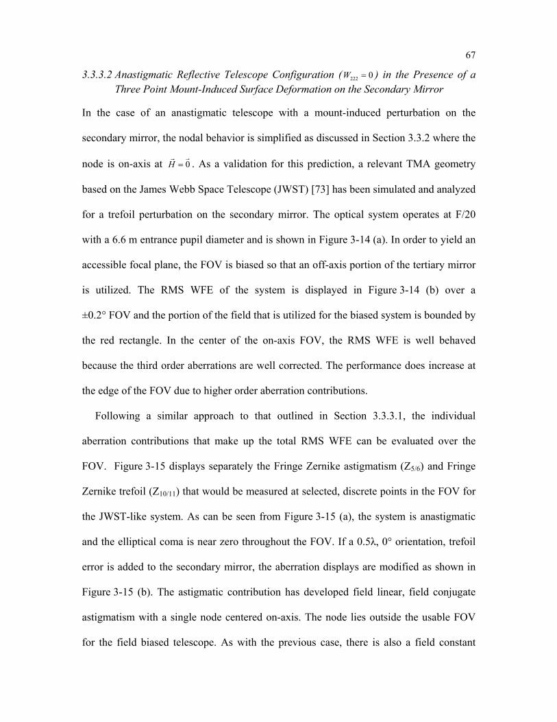
67
3.3.3.2 Anastigmatic Reflective Telescope Configuration ( 222 0W = ) in the Presence of a Three Point Mount-Induced Surface Deformation on the Secondary Mirror
In the case of an anastigmatic telescope with a mount-induced perturbation on the
secondary mirror, the nodal behavior is simplified as discussed in Section 3.3.2 where the
node is on-axis at 0H =
. As a validation for this prediction, a relevant TMA geometry
based on the James Webb Space Telescope (JWST) [73] has been simulated and analyzed
for a trefoil perturbation on the secondary mirror. The optical system operates at F/20
with a 6.6 m entrance pupil diameter and is shown in Figure 3-14 (a). In order to yield an
accessible focal plane, the FOV is biased so that an off-axis portion of the tertiary mirror
is utilized. The RMS WFE of the system is displayed in Figure 3-14 (b) over a
±0.2° FOV and the portion of the field that is utilized for the biased system is bounded by
the red rectangle. In the center of the on-axis FOV, the RMS WFE is well behaved
because the third order aberrations are well corrected. The performance does increase at
the edge of the FOV due to higher order aberration contributions.
Following a similar approach to that outlined in Section 3.3.3.1, the individual
aberration contributions that make up the total RMS WFE can be evaluated over the
FOV. Figure 3-15 displays separately the Fringe Zernike astigmatism (Z5/6) and Fringe
Zernike trefoil (Z10/11) that would be measured at selected, discrete points in the FOV for
the JWST-like system. As can be seen from Figure 3-15 (a), the system is anastigmatic
and the elliptical coma is near zero throughout the FOV. If a 0.5λ, 0° orientation, trefoil
error is added to the secondary mirror, the aberration displays are modified as shown in
Figure 3-15 (b). The astigmatic contribution has developed field linear, field conjugate
astigmatism with a single node centered on-axis. The node lies outside the usable FOV
for the field biased telescope. As with the previous case, there is also a field constant
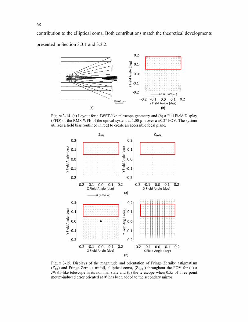
68
contribution to the elliptical coma. Both contributions match the theoretical developments
presented in Section 3.3.1 and 3.3.2.
-0.2000 -0.1000 0.0000 0.1000 0.2
000
000
000
000
000
1250.00 MM
(a) (b)
1250.00 mm
1
0.25λ (1.000µm)
Y Fi
eld
Angl
e (d
eg)
0.2
0.1
0.0
-0.1
-0.2
X Field Angle (deg)-0.2 -0.1 0.0 0.1 0.2
Figure 3-14. (a) Layout for a JWST-like telescope geometry and (b) a Full Field Display (FFD) of the RMS WFE of the optical system at 1.00 µm over a ±0.2° FOV. The system utilizes a field bias (outlined in red) to create an accessible focal plane.
-0.2000 -0.1000 0.0000 0.1000 0.2000
000
000
000
000
000
-0.2000 -0.1000 0.0000 0.1000 0.2000
000
000
000
000
000
-0.2000 -0.1000 0.0000 0.1000 0.2
000
000
000
000
000
-0.2000 -0.1000 0.0000 0.1000 0.2000
X Field Angle in Object Space - degrees
000
000
000
000
000
Y Fi
eld
Angl
e (d
eg)
0.2
0.1
0.0
-0.1
-0.2
X Field Angle (deg)-0.2 -0.1 0.0 0.1 0.2
Z10/11Z5/6
(a)
(b)
Y Fi
eld
Angl
e (d
eg)
0.2
0.1
0.0
-0.1
-0.2
X Field Angle (deg)-0.2 -0.1 0.0 0.1 0.2
Y Fi
eld
Angl
e (d
eg)
0.2
0.1
0.0
-0.1
-0.2
X Field Angle (deg)-0.2 -0.1 0.0 0.1 0.2
Y Fi
eld
Angl
e (d
eg)
0.2
0.1
0.0
-0.1
-0.2
X Field Angle (deg)-0.2 -0.1 0.0 0.1 0.2
1
1λ (1.000µm)
Figure 3-15. Displays of the magnitude and orientation of Fringe Zernike astigmatism (Z5/6) and Fringe Zernike trefoil, elliptical coma, (Z10/11) throughout the FOV for (a) a JWST-like telescope in its nominal state and (b) the telescope when 0.5λ of three point mount-induced error oriented at 0° has been added to the secondary mirror.
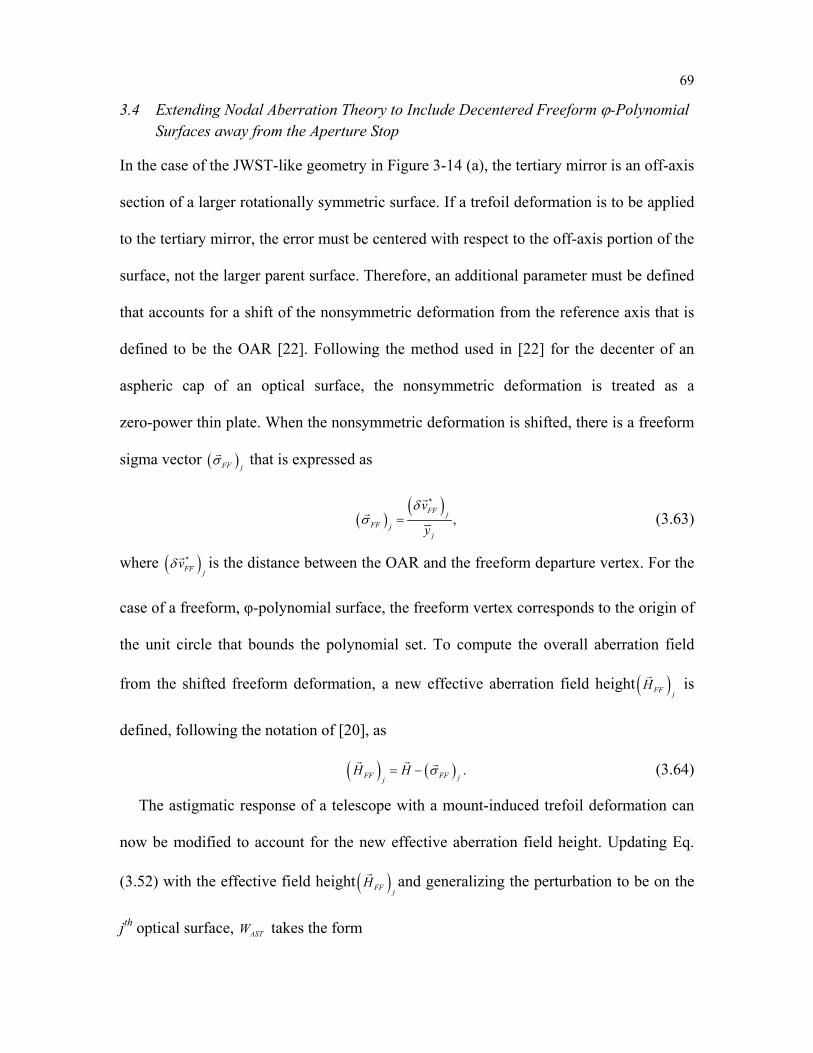
69
3.4 Extending Nodal Aberration Theory to Include Decentered Freeform ϕ-Polynomial Surfaces away from the Aperture Stop
In the case of the JWST-like geometry in Figure 3-14 (a), the tertiary mirror is an off-axis
section of a larger rotationally symmetric surface. If a trefoil deformation is to be applied
to the tertiary mirror, the error must be centered with respect to the off-axis portion of the
surface, not the larger parent surface. Therefore, an additional parameter must be defined
that accounts for a shift of the nonsymmetric deformation from the reference axis that is
defined to be the OAR [22]. Following the method used in [22] for the decenter of an
aspheric cap of an optical surface, the nonsymmetric deformation is treated as a
zero-power thin plate. When the nonsymmetric deformation is shifted, there is a freeform
sigma vector ( )FF jσ that is expressed as
( )( )*
,FF j
FF jj
v
y
δσ =
(3.63)
where ( )*FF j
vδ is the distance between the OAR and the freeform departure vertex. For the
case of a freeform, φ-polynomial surface, the freeform vertex corresponds to the origin of
the unit circle that bounds the polynomial set. To compute the overall aberration field
from the shifted freeform deformation, a new effective aberration field height ( )FF jH
is
defined, following the notation of [20], as
( ) ( ) .FF FF jjH H σ= −
(3.64)
The astigmatic response of a telescope with a mount-induced trefoil deformation can
now be modified to account for the new effective aberration field height. Updating Eq.
(3.52) with the effective field height ( )FF jH
and generalizing the perturbation to be on the
jth optical surface, ASTW takes the form
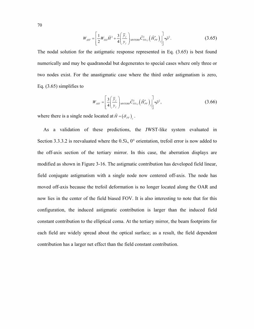
70
( )2 3 * 2222 333,
1 3 .2 4
jAST MNTERR j FF j
j
yW W H C H
yρ
= +
(3.65)
The nodal solution for the astigmatic response represented in Eq. (3.65) is best found
numerically and may be quadranodal but degenerates to special cases where only three or
two nodes exist. For the anastigmatic case where the third order astigmatism is zero,
Eq. (3.65) simplifies to
( )3 * 2333,
3 ,4
jAST MNTERR j FF j
j
yW C H
yρ
=
(3.66)
where there is a single node located at ( )FF jH σ=
.
As a validation of these predictions, the JWST-like system evaluated in
Section 3.3.3.2 is reevaluated where the 0.5λ, 0° orientation, trefoil error is now added to
the off-axis section of the tertiary mirror. In this case, the aberration displays are
modified as shown in Figure 3-16. The astigmatic contribution has developed field linear,
field conjugate astigmatism with a single node now centered off-axis. The node has
moved off-axis because the trefoil deformation is no longer located along the OAR and
now lies in the center of the field biased FOV. It is also interesting to note that for this
configuration, the induced astigmatic contribution is larger than the induced field
constant contribution to the elliptical coma. At the tertiary mirror, the beam footprints for
each field are widely spread about the optical surface; as a result, the field dependent
contribution has a larger net effect than the field constant contribution.
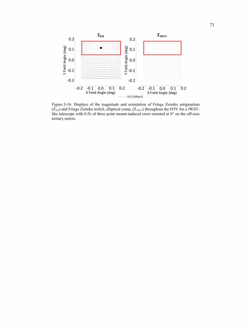
71
-0.2000 -0.1000 0.0000 0.1000 0.2000
X Field Angle in Object Space - degrees
0.2000
0.1000
0.0000
0.1000
0.2000
-0.2000 -0.1000 0.0000 0.1000 0.2000
X Field Angle in Object Space - degrees
-0.2000
-0.1000
0.0000
0.1000
0.2000
Y Fi
eld
Angl
e (d
eg)
0.2
0.1
0.0
-0.1
-0.2
X Field Angle (deg)-0.2 -0.1 0.0 0.1 0.2
Y Fi
eld
Angl
e (d
eg)
0.2
0.1
0.0
-0.1
-0.2
X Field Angle (deg)-0.2 -0.1 0.0 0.1 0.2
1
1λ (1.000µm)
Z10/11Z5/6
Figure 3-16. Displays of the magnitude and orientation of Fringe Zernike astigmatism (Z5/6) and Fringe Zernike trefoil, elliptical coma, (Z10/11) throughout the FOV for a JWST-like telescope with 0.5λ of three point mount-induced error oriented at 0° on the off-axis tertiary mirror.
72
Chapter 4. Experimental Validation of Nodal Aberration Theory for φ-Polynomial Optical Surfaces
Chapter 3 presented a theoretical foundation for the general, unrestricted aberration
theory for optical systems that employ φ-polynomial surfaces. In this chapter, this
theoretical foundation is verified experimentally by the design and implementation of an
aberration generating telescope. Within the basic telescope framework, a surface with a
φ-polynomial departure is placed in the optical path. When the surface is displaced
axially from the aperture stop of the optical system, aberrations of lower radial order than
the nonsymmetric departure of the surface are generated. The particular nonsymmetric
departure to be studied in this chapter is elliptical coma or Zernike trefoil. As will be
verified, when the trefoil surface is displaced from the stop surface, field conjugate, field
linear astigmatism is generated throughout the FOV. It will be shown that the aberration
is centered in the image plane about a point that depends on the lateral offset of the
Zernike trefoil vertex from the OAR of the telescope. Moreover, it will be verified that
the magnitude of the astigmatic aberration is generated linearly with relative axial
distance from the stop surface as predicted theoretically in Chapter 3.
4.1 Design of an Aberration Generating Schmidt Telescope
In its simplest form, a Schmidt telescope is composed of a spherical mirror, stop, and
aspheric corrector plate. The stop lies at the center of curvature of the spherical mirror so
that the system is corrected for third order coma and astigmatism. By placing a sixth
order aspheric corrector plate at the stop surface, the system is also corrected for third and
fifth order spherical aberration. In this configuration, the telescope is corrected for all
third order aberrations except field curvature and, as such, makes an excellent baseline
optical system for introducing controlled amounts of individual, isolated aberration types
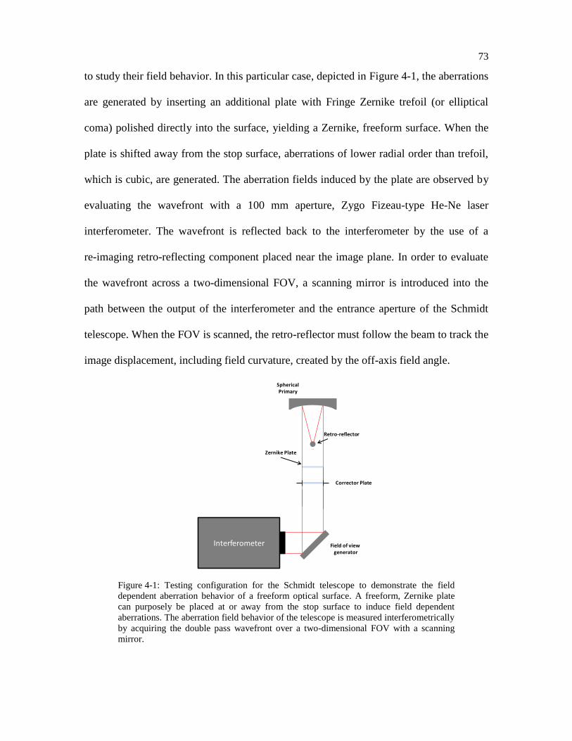
73
to study their field behavior. In this particular case, depicted in Figure 4-1, the aberrations
are generated by inserting an additional plate with Fringe Zernike trefoil (or elliptical
coma) polished directly into the surface, yielding a Zernike, freeform surface. When the
plate is shifted away from the stop surface, aberrations of lower radial order than trefoil,
which is cubic, are generated. The aberration fields induced by the plate are observed by
evaluating the wavefront with a 100 mm aperture, Zygo Fizeau-type He-Ne laser
interferometer. The wavefront is reflected back to the interferometer by the use of a
re-imaging retro-reflecting component placed near the image plane. In order to evaluate
the wavefront across a two-dimensional FOV, a scanning mirror is introduced into the
path between the output of the interferometer and the entrance aperture of the Schmidt
telescope. When the FOV is scanned, the retro-reflector must follow the beam to track the
image displacement, including field curvature, created by the off-axis field angle.
Interferometer Field of viewgenerator
Spherical Primary
Zernike Plate
Corrector Plate
Retro-reflector
Figure 4-1: Testing configuration for the Schmidt telescope to demonstrate the field
dependent aberration behavior of a freeform optical surface. A freeform, Zernike plate
can purposely be placed at or away from the stop surface to induce field dependent
aberrations. The aberration field behavior of the telescope is measured interferometrically
by acquiring the double pass wavefront over a two-dimensional FOV with a scanning
mirror.
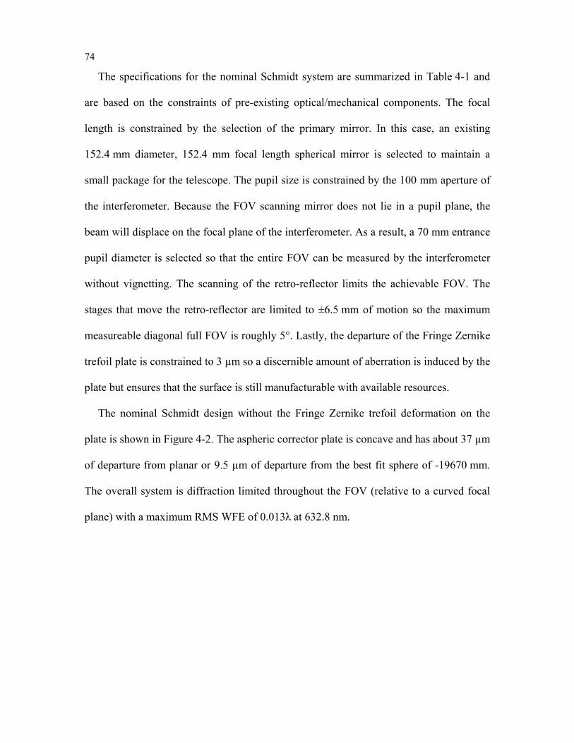
74
The specifications for the nominal Schmidt system are summarized in Table 4-1 and
are based on the constraints of pre-existing optical/mechanical components. The focal
length is constrained by the selection of the primary mirror. In this case, an existing
152.4 mm diameter, 152.4 mm focal length spherical mirror is selected to maintain a
small package for the telescope. The pupil size is constrained by the 100 mm aperture of
the interferometer. Because the FOV scanning mirror does not lie in a pupil plane, the
beam will displace on the focal plane of the interferometer. As a result, a 70 mm entrance
pupil diameter is selected so that the entire FOV can be measured by the interferometer
without vignetting. The scanning of the retro-reflector limits the achievable FOV. The
stages that move the retro-reflector are limited to ±6.5 mm of motion so the maximum
measureable diagonal full FOV is roughly 5°. Lastly, the departure of the Fringe Zernike
trefoil plate is constrained to 3 µm so a discernible amount of aberration is induced by the
plate but ensures that the surface is still manufacturable with available resources.
The nominal Schmidt design without the Fringe Zernike trefoil deformation on the
plate is shown in Figure 4-2. The aspheric corrector plate is concave and has about 37 µm
of departure from planar or 9.5 µm of departure from the best fit sphere of -19670 mm.
The overall system is diffraction limited throughout the FOV (relative to a curved focal
plane) with a maximum RMS WFE of 0.013λ at 632.8 nm.
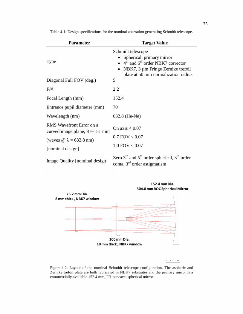
75
Table 4-1. Design specifications for the nominal aberration generating Schmidt telescope.
Parameter Target Value
Type
Schmidt telescope
Spherical, primary mirror
4th
and 6th
order NBK7 corrector
NBK7, 3 µm Fringe Zernike trefoil
plate at 50 mm normalization radius
Diagonal Full FOV (deg.) 5
F/# 2.2
Focal Length (mm) 152.4
Entrance pupil diameter (mm) 70
Wavelength (nm) 632.8 (He-Ne)
RMS Wavefront Error on a
curved image plane, R=-151 mm
(waves @ λ = 632.8 nm)
[nominal design]
On axis < 0.07
0.7 FOV < 0.07
1.0 FOV < 0.07
Image Quality [nominal design] Zero 3
rd and 5
th order spherical, 3
rd order
coma, 3rd
order astigmatism
16:57:01
F/2, Schmidt Scale: 0.60 KHF 02-Jan-14
41.67 MM
76.2 mm Dia.8 mm thick , NBK7 window
100 mm Dia.10 mm thick , NBK7 window
152.4 mm Dia.304.8 mm ROC Spherical Mirror
Figure 4-2. Layout of the nominal Schmidt telescope configuration. The aspheric and
Zernike trefoil plate are both fabricated in NBK7 substrates and the primary mirror is a
commercially available 152.4 mm, F/1 concave, spherical mirror.
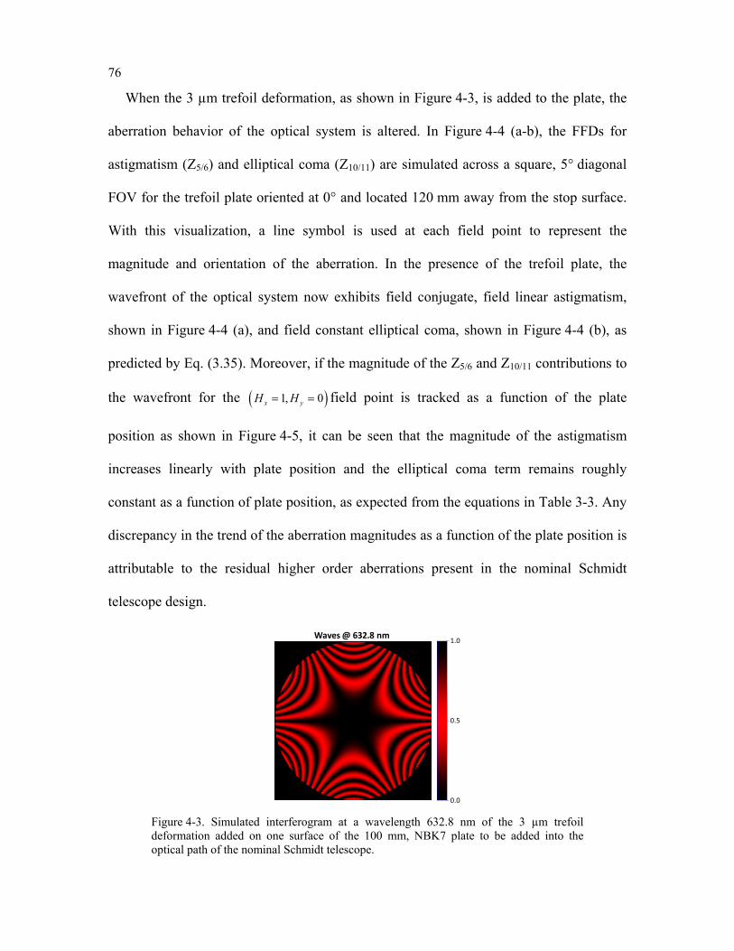
76
When the 3 µm trefoil deformation, as shown in Figure 4-3, is added to the plate, the
aberration behavior of the optical system is altered. In Figure 4-4 (a-b), the FFDs for
astigmatism (Z5/6) and elliptical coma (Z10/11) are simulated across a square, 5° diagonal
FOV for the trefoil plate oriented at 0° and located 120 mm away from the stop surface.
With this visualization, a line symbol is used at each field point to represent the
magnitude and orientation of the aberration. In the presence of the trefoil plate, the
wavefront of the optical system now exhibits field conjugate, field linear astigmatism,
shown in Figure 4-4 (a), and field constant elliptical coma, shown in Figure 4-4 (b), as
predicted by Eq. (3.35). Moreover, if the magnitude of the Z5/6 and Z10/11 contributions to
the wavefront for the ( )1, 0x yH H= = field point is tracked as a function of the plate
position as shown in Figure 4-5, it can be seen that the magnitude of the astigmatism
increases linearly with plate position and the elliptical coma term remains roughly
constant as a function of plate position, as expected from the equations in Table 3-3. Any
discrepancy in the trend of the aberration magnitudes as a function of the plate position is
attributable to the residual higher order aberrations present in the nominal Schmidt
telescope design.
Waves @ 632.8 nm 1.0
0.5
0.0
Figure 4-3. Simulated interferogram at a wavelength 632.8 nm of the 3 µm trefoil deformation added on one surface of the 100 mm, NBK7 plate to be added into the optical path of the nominal Schmidt telescope.
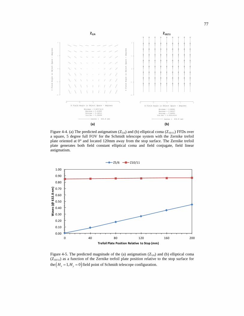
77
09:59:19
F/2, Schmidt
KHF 10-May-13
FRINGE ZERNIKE PAIR Z10 AND Z11
vs
FIELD ANGLE IN OBJECT SPACE
Minimum = 0.84881
Maximum = 0.84937
Average = 0.84905
Std Dev = 0.00014319
1waves ( 632.8 nm)
-2 -1 0 1 2
X Field Angle in Object Space - degrees
-2
-1
0
1
2
Y Field Angle in Object Space - degrees
09:59:19
F/2, Schmidt
KHF 10-May-13
FRINGE ZERNIKE PAIR Z10 AND Z11
vs
FIELD ANGLE IN OBJECT SPACE
Minimum = 0.84881
Maximum = 0.84937
Average = 0.84905
Std Dev = 0.00014319
1waves ( 632.8 nm)
-2 -1 0 1 2
X Field Angle in Object Space - degrees
-2
-1
0
1
2
Y Field Angle in Object Space - degrees
09:59:43
F/2, Schmidt
KHF 10-May-13
FRINGE ZERNIKE PAIR Z5 AND Z6
vs
FIELD ANGLE IN OBJECT SPACE
Minimum = 0.66717e-6
Maximum = 0.41885
Average = 0.24015
Std Dev = 0.08969
1waves ( 632.8 nm)
-2 -1 0 1 2
X Field Angle in Object Space - degrees
-2
-1
0
1
2
Y Field Angle in Object Space - degrees
09:59:43
F/2, Schmidt
KHF 10-May-13
FRINGE ZERNIKE PAIR Z5 AND Z6
vs
FIELD ANGLE IN OBJECT SPACE
Minimum = 0.66717e-6
Maximum = 0.41885
Average = 0.24015
Std Dev = 0.08969
1waves ( 632.8 nm)
-2 -1 0 1 2
X Field Angle in Object Space - degrees
-2
-1
0
1
2
Y Field Angle in Object Space - degrees
09:59:19
F/2, Schmidt
KHF 10-May-13
FRINGE ZERNIKE PAIR Z10 AND Z11
vs
FIELD ANGLE IN OBJECT SPACE
Minimum = 0.84881
Maximum = 0.84937
Average = 0.84905
Std Dev = 0.00014319
1waves ( 632.8 nm)
-2 -1 0 1 2
X Field Angle in Object Space - degrees
-2
-1
0
1
2
Y Field Angle in Object Space - degrees
Z5/6 Z10/11
(a) (b)
09:59:43
F/2, Schmidt
KHF 10-May-13
FRINGE ZERNIKE PAIR Z5 AND Z6
vs
FIELD ANGLE IN OBJECT SPACE
Minimum = 0.66717e-6
Maximum = 0.41885
Average = 0.24015
Std Dev = 0.08969
1waves ( 632.8 nm)
-2 -1 0 1 2
X Field Angle in Object Space - degrees
-2
-1
0
1
2
Y Field Angle in Object Space - degrees
Figure 4-4. (a) The predicted astigmatism (Z5/6) and (b) elliptical coma (Z10/11) FFDs over
a square, 5 degree full FOV for the Schmidt telescope system with the Zernike trefoil
plate oriented at 0° and located 120mm away from the stop surface. The Zernike trefoil
plate generates both field constant elliptical coma and field conjugate, field linear
astigmatism.
0.00
0.10
0.20
0.30
0.40
0.50
0.60
0.70
0.80
0.90
1.00
0 40 80 120 160 200
Wav
es
(@ 6
32
.8 n
m)
Trefoil Plate Position Relative to Stop (mm)
Z5/6 Z10/11
Figure 4-5. The predicted magnitude of the (a) astigmatism (Z5/6) and (b) elliptical coma
(Z10/11) as a function of the Zernike trefoil plate position relative to the stop surface for
the 1, 0x yH H field point of Schmidt telescope configuration.
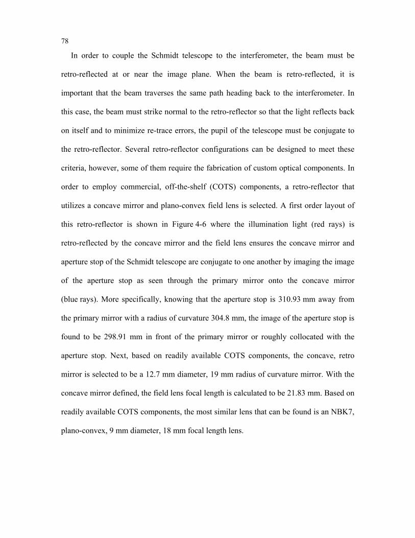
78
In order to couple the Schmidt telescope to the interferometer, the beam must be
retro-reflected at or near the image plane. When the beam is retro-reflected, it is
important that the beam traverses the same path heading back to the interferometer. In
this case, the beam must strike normal to the retro-reflector so that the light reflects back
on itself and to minimize re-trace errors, the pupil of the telescope must be conjugate to
the retro-reflector. Several retro-reflector configurations can be designed to meet these
criteria, however, some of them require the fabrication of custom optical components. In
order to employ commercial, off-the-shelf (COTS) components, a retro-reflector that
utilizes a concave mirror and plano-convex field lens is selected. A first order layout of
this retro-reflector is shown in Figure 4-6 where the illumination light (red rays) is
retro-reflected by the concave mirror and the field lens ensures the concave mirror and
aperture stop of the Schmidt telescope are conjugate to one another by imaging the image
of the aperture stop as seen through the primary mirror onto the concave mirror
(blue rays). More specifically, knowing that the aperture stop is 310.93 mm away from
the primary mirror with a radius of curvature 304.8 mm, the image of the aperture stop is
found to be 298.91 mm in front of the primary mirror or roughly collocated with the
aperture stop. Next, based on readily available COTS components, the concave, retro
mirror is selected to be a 12.7 mm diameter, 19 mm radius of curvature mirror. With the
concave mirror defined, the field lens focal length is calculated to be 21.83 mm. Based on
readily available COTS components, the most similar lens that can be found is an NBK7,
plano-convex, 9 mm diameter, 18 mm focal length lens.
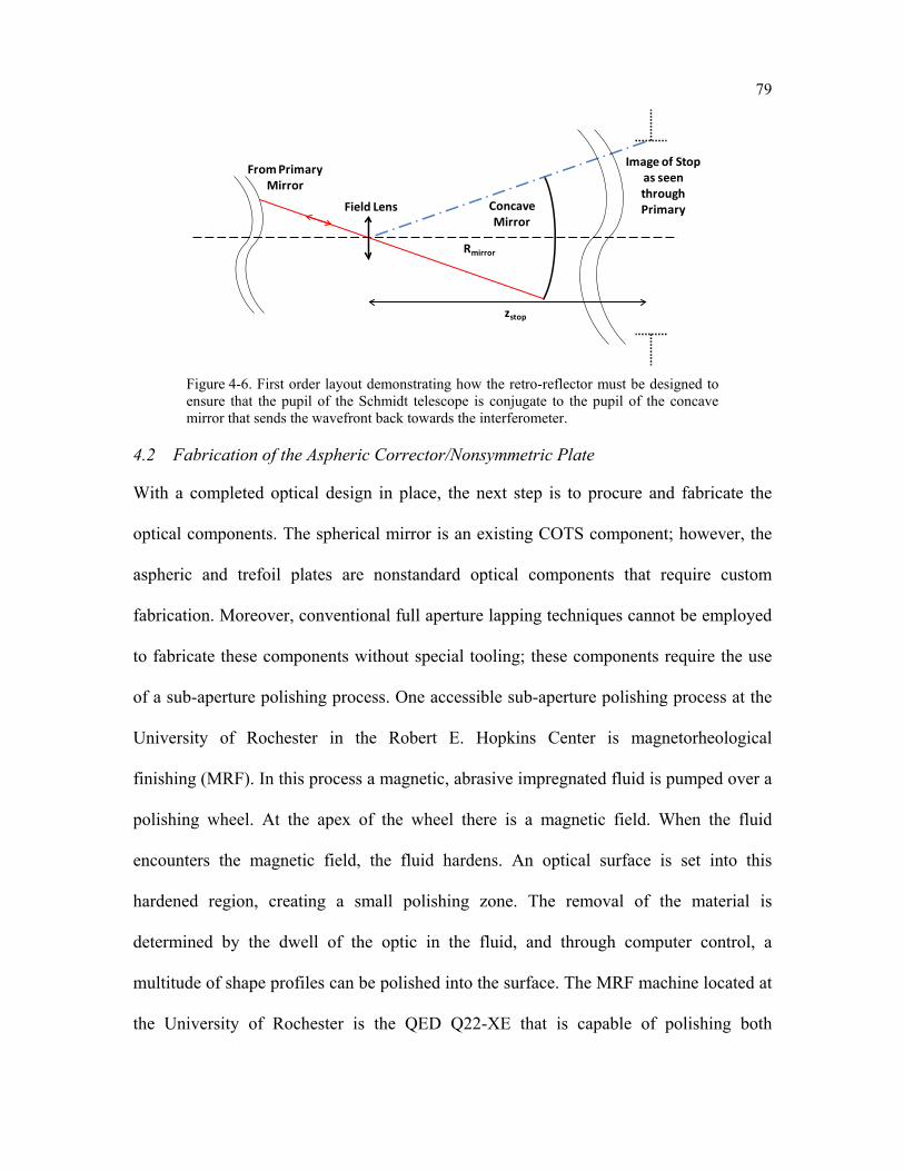
79
ConcaveMirror
Field Lens
Rmirror
Image of Stop as seen through Primary
From Primary Mirror
zstop
Figure 4-6. First order layout demonstrating how the retro-reflector must be designed to ensure that the pupil of the Schmidt telescope is conjugate to the pupil of the concave mirror that sends the wavefront back towards the interferometer.
4.2 Fabrication of the Aspheric Corrector/Nonsymmetric Plate
With a completed optical design in place, the next step is to procure and fabricate the
optical components. The spherical mirror is an existing COTS component; however, the
aspheric and trefoil plates are nonstandard optical components that require custom
fabrication. Moreover, conventional full aperture lapping techniques cannot be employed
to fabricate these components without special tooling; these components require the use
of a sub-aperture polishing process. One accessible sub-aperture polishing process at the
University of Rochester in the Robert E. Hopkins Center is magnetorheological
finishing (MRF). In this process a magnetic, abrasive impregnated fluid is pumped over a
polishing wheel. At the apex of the wheel there is a magnetic field. When the fluid
encounters the magnetic field, the fluid hardens. An optical surface is set into this
hardened region, creating a small polishing zone. The removal of the material is
determined by the dwell of the optic in the fluid, and through computer control, a
multitude of shape profiles can be polished into the surface. The MRF machine located at
the University of Rochester is the QED Q22-XE that is capable of polishing both
80
rotationally symmetric and nonsymmetric surfaces up to 100 mm in diameter and is well
suited for polishing the aspheric and trefoil plates.
The NBK7 substrates for fabrication are COTS pre-polished flats to λ/4 or better. The
aspheric plate substrate is 76.2 mm in diameter and 8 mm thick whereas the trefoil plate
substrate is 100 mm in diameter and 10 mm thick. For each plate only one surface is to be
polished by the MRF machine. In order to create the dwell maps for polishing, the
removal within the polishing zone must be known. To determine this removal, four spots
are polished into a sacrificial 50 mm NBK7 substrate and characterized by a Zygo laser
interferometer with a transmission reference flat attached. Once the removal of the
polishing zone has been characterized, the machine computes from the initial surface
shape a dwell map to create the desired final surface shape. Because a large amount of
material needs to be removed for both plates and the removal rate of MRF is generally
small, the polishing is split into multiple runs. During each run only part of the overall
departure is polished into the surface. With this method, the polishing runtimes are
shorter, providing better stability of the polishing parameters during fabrication. After
each polishing run, the plates are measured with an interferometer in reflection or
transmission if the departure of the surface from planar is too great. The measurement
after each polishing run serves as the input for the subsequent polishing cycle.
The final surface shape of the third and fifth order aspheric correcting plate and its
residual from the theoretical design are shown in Figure 4-7 (a-b) over a 70 mm clear
aperture. As depicted in Figure 4-7 (a), roughly 26.6 µm peak-to-valley (PV) of departure
has been polished into the substrate material over the course of fourteen polishing runs
that were each removing 2 µm PV. The residual error after polishing, Figure 4-7 (b), is
81
about 0.56λ PV or 0.066λ RMS at the testing wavelength of 632.8 nm. There is some
coma present in the surface but most of the residual is higher order and present at the
edges where the slopes are largest. A small center feature as well as a spoking pattern (a
mid-spatial frequency error) is observed. Both features are a residual from the sub-
aperture MRF polishing process that is difficult to correct once polished into the part.
However, since the measured errors are higher order and not low order astigmatism, it
will not impact or prevent any features to be observed during the measurement of the
assembled Schmidt optical system.
(a) (b)
Figure 4-7. (a) Measured surface departure of the aspheric corrector plate for the Schmidt telescope and (b) residual error when the nominal optical design surface is subtracted from the measured surface. The error is about 0.56λ PV or 0.066λ RMS at the testing wavelength of 632.8 nm.
For the trefoil plate, the final shape and its residual from theoretical are shown in
Figure 4-8 (a-b) over a 98 mm clear aperture. The surface departure of the final surface,
Figure 4-8 (a), is 5.75 µm PV and has been polished in over the course of seven runs that
each removed about 1.2 µm of material. The residual for this surface, Figure 4-8 (b), is
0.30λ PV or 0.05λ RMS. Similar to the case with the asphere, the residual is primarily
higher order with a center artifact and a mid-spatial frequency spoking pattern. Some
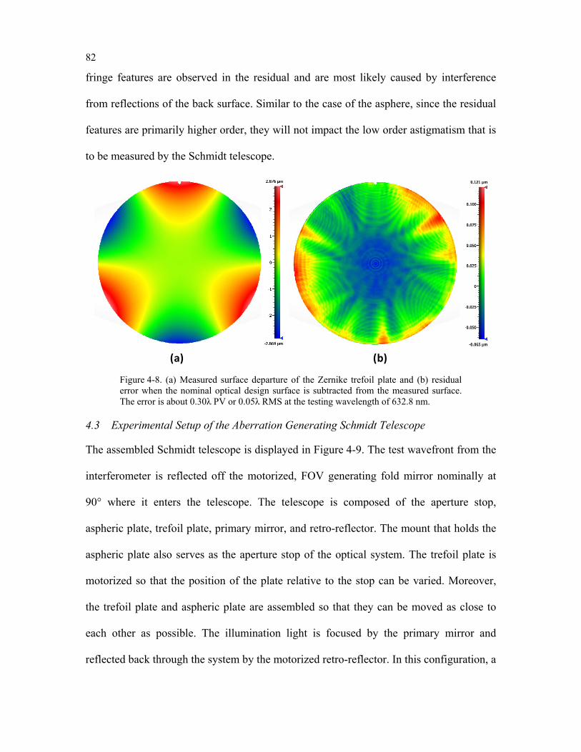
82
fringe features are observed in the residual and are most likely caused by interference
from reflections of the back surface. Similar to the case of the asphere, since the residual
features are primarily higher order, they will not impact the low order astigmatism that is
to be measured by the Schmidt telescope.
(a) (b)
Figure 4-8. (a) Measured surface departure of the Zernike trefoil plate and (b) residual error when the nominal optical design surface is subtracted from the measured surface. The error is about 0.30λ PV or 0.05λ RMS at the testing wavelength of 632.8 nm.
4.3 Experimental Setup of the Aberration Generating Schmidt Telescope
The assembled Schmidt telescope is displayed in Figure 4-9. The test wavefront from the
interferometer is reflected off the motorized, FOV generating fold mirror nominally at
90° where it enters the telescope. The telescope is composed of the aperture stop,
aspheric plate, trefoil plate, primary mirror, and retro-reflector. The mount that holds the
aspheric plate also serves as the aperture stop of the optical system. The trefoil plate is
motorized so that the position of the plate relative to the stop can be varied. Moreover,
the trefoil plate and aspheric plate are assembled so that they can be moved as close to
each other as possible. The illumination light is focused by the primary mirror and
reflected back through the system by the motorized retro-reflector. In this configuration, a
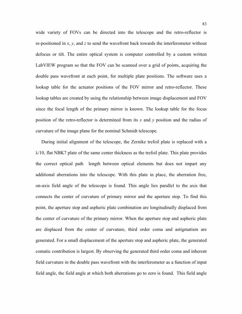
83
wide variety of FOVs can be directed into the telescope and the retro-reflector is
re-positioned in x, y, and z to send the wavefront back towards the interferometer without
defocus or tilt. The entire optical system is computer controlled by a custom written
LabVIEW program so that the FOV can be scanned over a grid of points, acquiring the
double pass wavefront at each point, for multiple plate positions. The software uses a
lookup table for the actuator positions of the FOV mirror and retro-reflector. These
lookup tables are created by using the relationship between image displacement and FOV
since the focal length of the primary mirror is known. The lookup table for the focus
position of the retro-reflector is determined from its x and y position and the radius of
curvature of the image plane for the nominal Schmidt telescope.
During initial alignment of the telescope, the Zernike trefoil plate is replaced with a
λ/10, flat NBK7 plate of the same center thickness as the trefoil plate. This plate provides
the correct optical path length between optical elements but does not impart any
additional aberrations into the telescope. With this plate in place, the aberration free,
on-axis field angle of the telescope is found. This angle lies parallel to the axis that
connects the center of curvature of primary mirror and the aperture stop. To find this
point, the aperture stop and aspheric plate combination are longitudinally displaced from
the center of curvature of the primary mirror. When the aperture stop and aspheric plate
are displaced from the center of curvature, third order coma and astigmatism are
generated. For a small displacement of the aperture stop and aspheric plate, the generated
comatic contribution is largest. By observing the generated third order coma and inherent
field curvature in the double pass wavefront with the interferometer as a function of input
field angle, the field angle at which both aberrations go to zero is found. This field angle
84
corresponds to the aberration free, on-axis field angle. Once the on-axis field is found, the
wavefront of an off-axis field angle is observed with the interferometer. The aspheric
plate is now translated longitudinally until the coma in the wavefront is zero at the
interrogated field point as well as throughout the entire FOV. This step ensures that the
aperture stop and aspheric plate are now again at the center of curvature of the primary
mirror.
With the telescope aligned and the on-axis field angle determined, the Zernike plate is
placed into the optical path, replacing the surrogate NBK7 plate. The Zernike plate is
aligned so that the generated field conjugate, linear astigmatism for a plate position away
from the stop is roughly zero on-axis. In addition, the orientation of the Zernike plate is
determined by evaluating the Z10 contribution to Zernike trefoil and adjusting the
orientation of the plate until this term is zero. This equates to an orientation of 0° for the
Zernike plate. With the plate aligned, the experiment proceeds. The LabVIEW program
cycles through five longitudinal Zernike plate positions. The first plate position is
roughly 10 mm away from the stop surface and the other plate positions are equally
spaced at roughly 20 mm increments. At each plate position, the program acquires ten
wavefront measurements with a one second difference between measurements over a 9x9
grid throughout the FOV. Averaging multiple measurements over time helps reduce the
effects of vibration and air turbulence on the overall measurement since the
interferometric cavity is long and there are many mounted optical components that lie in
the optical path.
In addition to acquiring a set of interferograms over a 9x9 grid of field points with the
Zernike plate in the Schmidt telescope, a baseline measurement is also acquired with the
85
flat plate in the telescope over the same field grid. This baseline measurement is
subtracted from the Zernike plate measurement set as it accounts for any residual
misalignment induced aberrations present in the telescope configuration as well as the
surface figure error of the folding mirror that generates the FOV for the telescope. This
baseline subtraction ensures that the analyzed wavefront only reflects the aberrations
induced by the trefoil plate.
Zygo Interferometer
Primary Mirror
TrefoilPlate
AsphericPlate
FOV Mirror
Retro-Reflector
Figure 4-9. Experimental setup of the Schmidt telescope system. The scanning mirror and retro-reflector are motorized so that the FOV can be scanned over a two-dimensional grid of points. The trefoil plate is also motorized so that effect of plate position on magnitude of generated aberration field can be studied.
4.4 Experimental Results
4.4.1 The Generated Field Conjugate, Field Linear Astigmatic Field
As an example of the measurement process, a 3x3 grid of wavefronts spanning a square,
5° diagonal FOV is shown in Figure 4-10 (a). The data shown is the difference at each
field point between the baseline measurement with the flat plate and the actual
measurement with the Zernike plate oriented at 0° and displaced approximately 100 mm
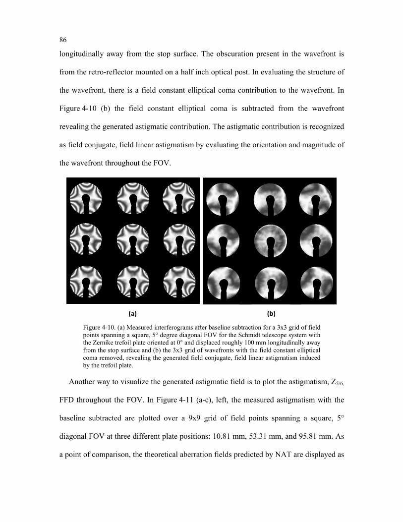
86
longitudinally away from the stop surface. The obscuration present in the wavefront is
from the retro-reflector mounted on a half inch optical post. In evaluating the structure of
the wavefront, there is a field constant elliptical coma contribution to the wavefront. In
Figure 4-10 (b) the field constant elliptical coma is subtracted from the wavefront
revealing the generated astigmatic contribution. The astigmatic contribution is recognized
as field conjugate, field linear astigmatism by evaluating the orientation and magnitude of
the wavefront throughout the FOV.
(a) (b)
Figure 4-10. (a) Measured interferograms after baseline subtraction for a 3x3 grid of field points spanning a square, 5° degree diagonal FOV for the Schmidt telescope system with the Zernike trefoil plate oriented at 0° and displaced roughly 100 mm longitudinally away from the stop surface and (b) the 3x3 grid of wavefronts with the field constant elliptical coma removed, revealing the generated field conjugate, field linear astigmatism induced by the trefoil plate.
Another way to visualize the generated astigmatic field is to plot the astigmatism, Z5/6,
FFD throughout the FOV. In Figure 4-11 (a-c), left, the measured astigmatism with the
baseline subtracted are plotted over a 9x9 grid of field points spanning a square, 5°
diagonal FOV at three different plate positions: 10.81 mm, 53.31 mm, and 95.81 mm. As
a point of comparison, the theoretical aberration fields predicted by NAT are displayed as
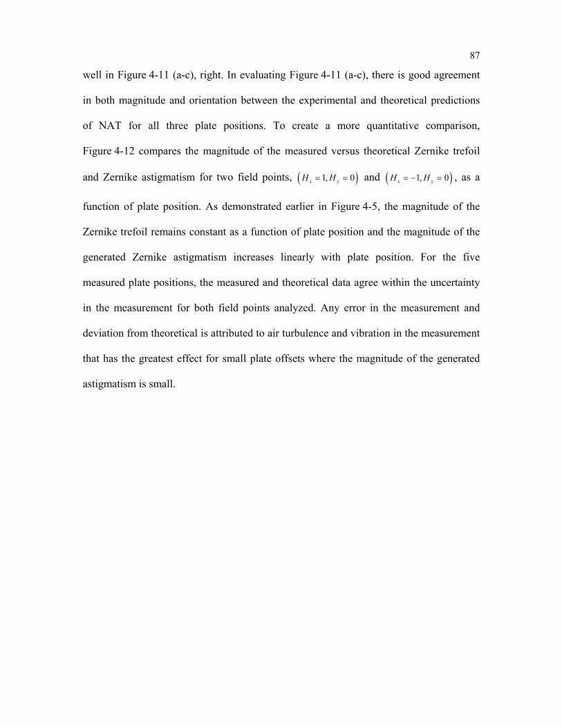
87
well in Figure 4-11 (a-c), right. In evaluating Figure 4-11 (a-c), there is good agreement
in both magnitude and orientation between the experimental and theoretical predictions
of NAT for all three plate positions. To create a more quantitative comparison,
Figure 4-12 compares the magnitude of the measured versus theoretical Zernike trefoil
and Zernike astigmatism for two field points, ( )1, 0x yH H= = and ( )1, 0x yH H= − = , as a
function of plate position. As demonstrated earlier in Figure 4-5, the magnitude of the
Zernike trefoil remains constant as a function of plate position and the magnitude of the
generated Zernike astigmatism increases linearly with plate position. For the five
measured plate positions, the measured and theoretical data agree within the uncertainty
in the measurement for both field points analyzed. Any error in the measurement and
deviation from theoretical is attributed to air turbulence and vibration in the measurement
that has the greatest effect for small plate offsets where the magnitude of the generated
astigmatism is small.
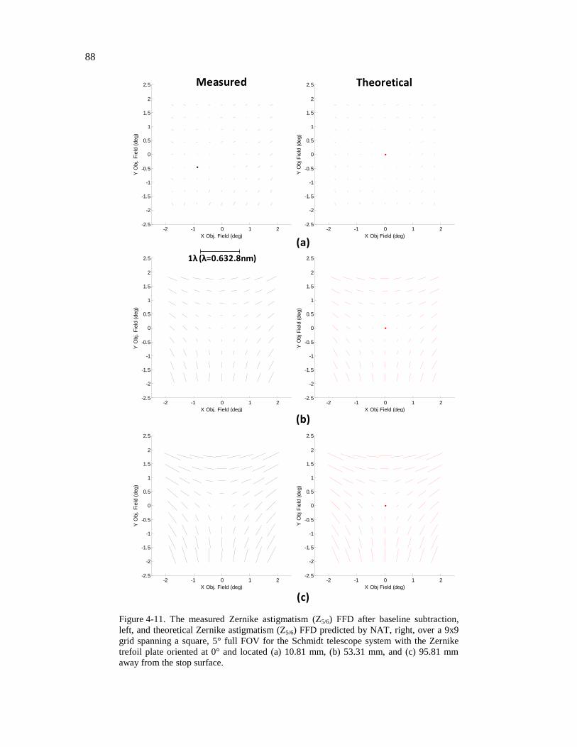
88
-2 -1 0 1 2-2.5
-2
-1.5
-1
-0.5
0
0.5
1
1.5
2
2.5
X Obj Field (deg)
Y O
bj F
ield
(deg)
-2 -1 0 1 2-2.5
-2
-1.5
-1
-0.5
0
0.5
1
1.5
2
2.5
X Obj. Field (deg)
Y O
bj. F
ield
(deg)
-2 -1 0 1 2-2.5
-2
-1.5
-1
-0.5
0
0.5
1
1.5
2
2.5
X Obj Field (deg)
Y O
bj F
ield
(deg)
-2 -1 0 1 2-2.5
-2
-1.5
-1
-0.5
0
0.5
1
1.5
2
2.5
X Obj. Field (deg)
Y O
bj. F
ield
(deg)
-2 -1 0 1 2-2.5
-2
-1.5
-1
-0.5
0
0.5
1
1.5
2
2.5
X Obj Field (deg)
Y O
bj F
ield
(deg)
-2 -1 0 1 2-2.5
-2
-1.5
-1
-0.5
0
0.5
1
1.5
2
2.5
X Obj. Field (deg)
Y O
bj. F
ield
(deg)
1λ (λ=0.632.8nm)
Experimental Theoretical
(a)
(b)
(c)
Measured
Figure 4-11. The measured Zernike astigmatism (Z5/6) FFD after baseline subtraction,
left, and theoretical Zernike astigmatism (Z5/6) FFD predicted by NAT, right, over a 9x9
grid spanning a square, 5° full FOV for the Schmidt telescope system with the Zernike
trefoil plate oriented at 0° and located (a) 10.81 mm, (b) 53.31 mm, and (c) 95.81 mm
away from the stop surface.
89
0 10 20 30 40 50 60 70 80 90 100 110
0
0.1
0.2
0.3
0.4
0.5
0.6
0.7
0.8
0.9
1
Plate Position (mm)
Mag
nitu
de (w
aves
at 6
32.8
nm
)
H=(-1,0)H=( 1,0)Theoretical
Zernike Trefoil
Zernike Astigmatism
Figure 4-12. Plot of the mean magnitude of the Zernike trefoil and astigmatism after baseline subtraction for two field points, ( )1, 0x yH H= = represented by the blue circle
and ( )1, 0x yH H= − = represented by the red star, for five measured plate positions. The error bars on the data points represent plus or minus one standard deviation from the mean value over the ten measurements acquired at each plate position. In black, the magnitude of the Zernike trefoil and astigmatism based on the theoretical predictions of NAT is plotted as a function of plate position.
4.4.2 Rotation of the Aberration Generating Plate
In Section 4.4.1, the Zernike plate in the Schmidt telescope configuration was aligned
on-axis and oriented at 0°. If the Zernike plate is now rotated, the orientation of the
astigmatic line images throughout the FOV will also rotate. To demonstrate this effect,
the Zernike plate in the Schmidt telescope is rotated 45° and the experiment is repeated to
acquire the wavefront throughout the FOV. Figure 4-13 (a) displays the measured results
for the rotated Zernike plate at 45° when the plate is roughly 100 mm away from the stop
surface and Figure 4-13 (b) displays the theoretical predictions from NAT. Similar to the
results shown earlier for a plate on-axis and oriented at 0°, there is very good agreement
between the measured astigmatic field and the theoretical simulations. In both cases, the
zero of the field conjugate, field linear astigmatism stays nearly on-axis and the line
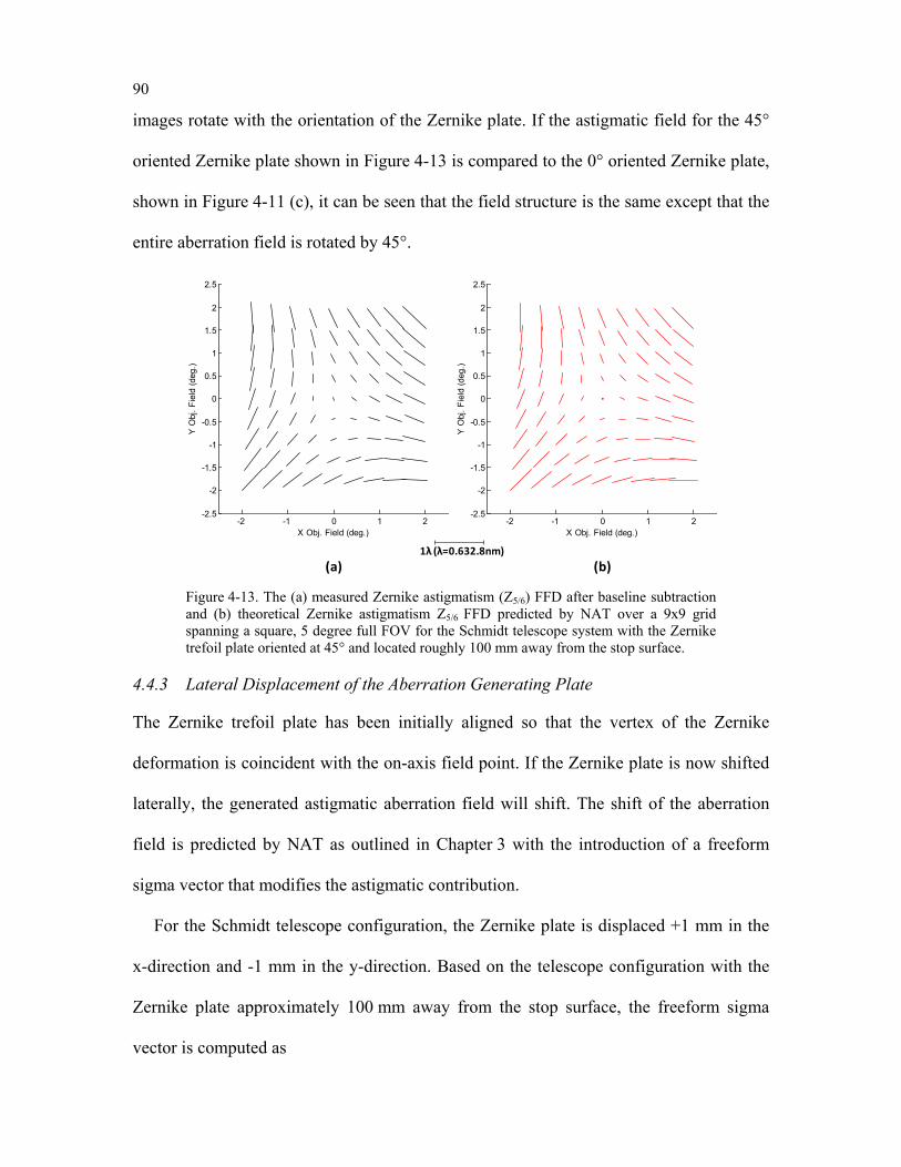
90
images rotate with the orientation of the Zernike plate. If the astigmatic field for the 45°
oriented Zernike plate shown in Figure 4-13 is compared to the 0° oriented Zernike plate,
shown in Figure 4-11 (c), it can be seen that the field structure is the same except that the
entire aberration field is rotated by 45°.
-2 -1 0 1 2-2.5
-2
-1.5
-1
-0.5
0
0.5
1
1.5
2
2.5
X Obj. Field (deg.)
Y O
bj. F
ield
(deg
.)
-2 -1 0 1 2-2.5
-2
-1.5
-1
-0.5
0
0.5
1
1.5
2
2.5
X Obj. Field (deg.)
Y O
bj. F
ield
(deg
.)
1λ (λ=0.632.8nm)(a) (b)
Figure 4-13. The (a) measured Zernike astigmatism (Z5/6) FFD after baseline subtraction and (b) theoretical Zernike astigmatism Z5/6 FFD predicted by NAT over a 9x9 grid spanning a square, 5 degree full FOV for the Schmidt telescope system with the Zernike trefoil plate oriented at 45° and located roughly 100 mm away from the stop surface.
4.4.3 Lateral Displacement of the Aberration Generating Plate
The Zernike trefoil plate has been initially aligned so that the vertex of the Zernike
deformation is coincident with the on-axis field point. If the Zernike plate is now shifted
laterally, the generated astigmatic aberration field will shift. The shift of the aberration
field is predicted by NAT as outlined in Chapter 3 with the introduction of a freeform
sigma vector that modifies the astigmatic contribution.
For the Schmidt telescope configuration, the Zernike plate is displaced +1 mm in the
x-direction and -1 mm in the y-direction. Based on the telescope configuration with the
Zernike plate approximately 100 mm away from the stop surface, the freeform sigma
vector is computed as
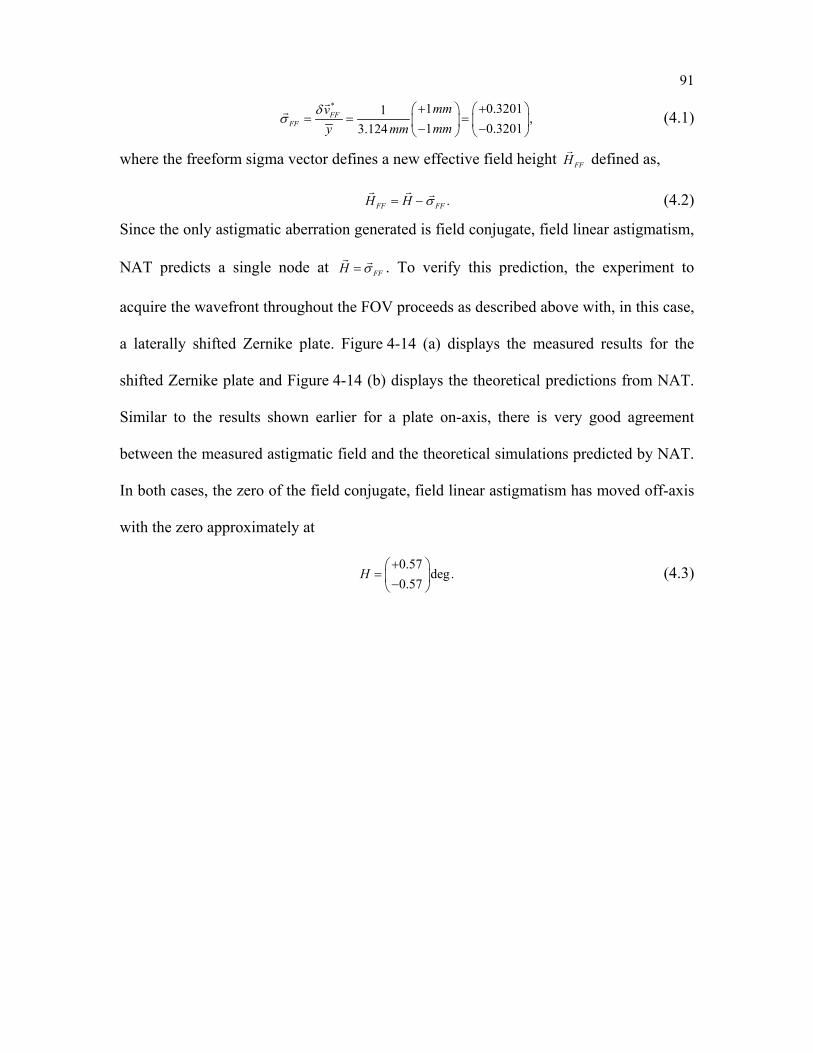
91
* 1 0.32011 ,
1 0.32013.124FF
FF
mmvmmy mm
δσ
+ + = = = − −
(4.1)
where the freeform sigma vector defines a new effective field height FFH
defined as,
.FF FFH H σ= −
(4.2)
Since the only astigmatic aberration generated is field conjugate, field linear astigmatism,
NAT predicts a single node at FFH σ=
. To verify this prediction, the experiment to
acquire the wavefront throughout the FOV proceeds as described above with, in this case,
a laterally shifted Zernike plate. Figure 4-14 (a) displays the measured results for the
shifted Zernike plate and Figure 4-14 (b) displays the theoretical predictions from NAT.
Similar to the results shown earlier for a plate on-axis, there is very good agreement
between the measured astigmatic field and the theoretical simulations predicted by NAT.
In both cases, the zero of the field conjugate, field linear astigmatism has moved off-axis
with the zero approximately at
0.57deg.
0.57H
+ = −
(4.3)
92
-2 -1 0 1 2-2.5
-2
-1.5
-1
-0.5
0
0.5
1
1.5
2
2.5
X Obj. Field (deg.)
Y O
bj. F
ield
(deg
.)
-2 -1 0 1 2-2.5
-2
-1.5
-1
-0.5
0
0.5
1
1.5
2
2.5
X Obj. Field (deg.)
Y O
bj. F
ield
(deg
.)
1λ (λ=0.632.8nm)(a) (b)
Figure 4-14. The (a) measured Zernike astigmatism (Z5/6) FFD after baseline subtraction and (b) theoretical Zernike astigmatism (Z5/6) FFD predicted by NAT over a 9x9 grid spanning a square, 5 degree full FOV for the Schmidt telescope system with the Zernike trefoil plate oriented at 0°, located roughly 100 mm away from the stop surface, and displaced laterally 1 mm in the x-direction and -1 mm in the y-direction.
93
Chapter 5. Design of a Freeform Unobscured Reflective Imager Employing φ-Polynomial Optical Surfaces
Historically, optical designers had a reputation for designing optical systems that exceed
the industry capabilities for fabrication and/or assembly. In general, these systems were
intrinsically rotationally symmetric using spheres, aspheres, or off-axis segments of a
rotationally symmetric surface (other than the occasional use of cylindrical or toric
surfaces for special case anamorphic systems). Recently, the optical fabrication industry
changed this paradigm by implementing a capability to fabricate diamond turned, optical
quality surfaces in the LWIR that are not rotationally symmetric. In particular, it is now
possible to fabricate an optical surface that is defined as a conic plus the lower order
terms of a Zernike polynomial (less than Fringe term 16).
In this chapter, an optical system design that is composed of tilted Zernike polynomial
mirrors is optimized to create a compact, LWIR optical system that will couple to a
320x256 pixel, 25 µm pixel pitch, uncooled microbolometer detector. The optimization
strategies that are employed during the optical design of this nonsymmetric system use
the principles of NAT applied to Zernike polynomial optical surfaces, as described in
Chapter 3. With this new understanding of freeform optical surfaces and their intrinsic
aberration fields, it is now possible to apply a NAT based optical analysis approach to
optimization.
5.1 The New Method of Optical Design
In the 1960s, the first optical designs that involved three or more mirrors in an
unobscured configuration started to be declassified and began to appear in limited
distribution government reports [74]. Motivated by the advance in LWIR detectors and
the accompanying need for stray light control, a number of systems were designed as
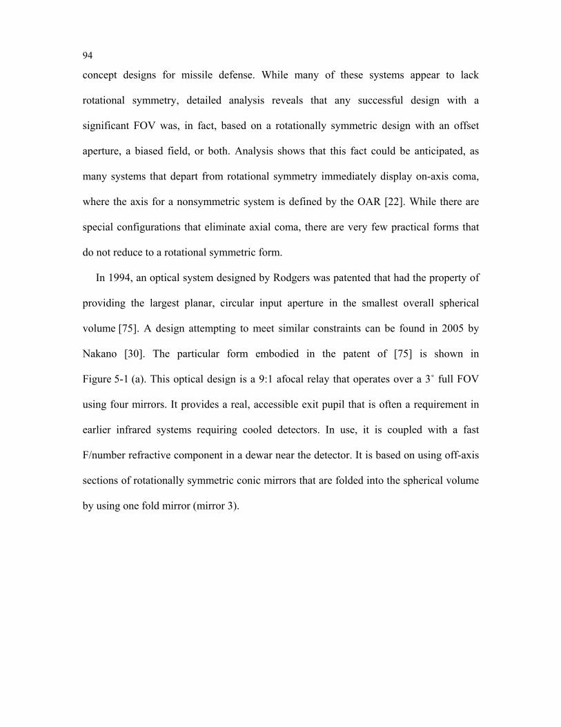
94
concept designs for missile defense. While many of these systems appear to lack
rotational symmetry, detailed analysis reveals that any successful design with a
significant FOV was, in fact, based on a rotationally symmetric design with an offset
aperture, a biased field, or both. Analysis shows that this fact could be anticipated, as
many systems that depart from rotational symmetry immediately display on-axis coma,
where the axis for a nonsymmetric system is defined by the OAR [22]. While there are
special configurations that eliminate axial coma, there are very few practical forms that
do not reduce to a rotational symmetric form.
In 1994, an optical system designed by Rodgers was patented that had the property of
providing the largest planar, circular input aperture in the smallest overall spherical
volume [75]. A design attempting to meet similar constraints can be found in 2005 by
Nakano [30]. The particular form embodied in the patent of [75] is shown in
Figure 5-1 (a). This optical design is a 9:1 afocal relay that operates over a 3˚ full FOV
using four mirrors. It provides a real, accessible exit pupil that is often a requirement in
earlier infrared systems requiring cooled detectors. In use, it is coupled with a fast
F/number refractive component in a dewar near the detector. It is based on using off-axis
sections of rotationally symmetric conic mirrors that are folded into the spherical volume
by using one fold mirror (mirror 3).
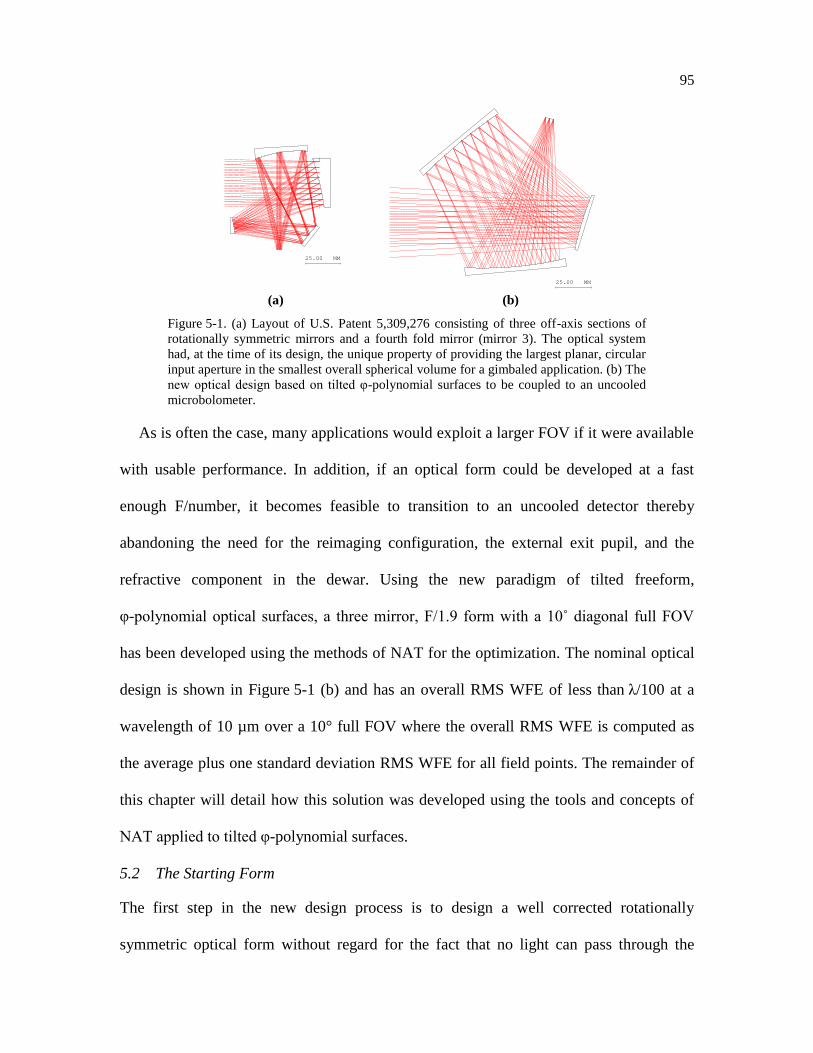
95
(a) (b)
14:37:35
AFOCAL 9:1 PUPIL DEMAG, 3x3 deg. FULL SCALE ORA 17-Sep-11
25.00 MM
14:25:51
Zernike Polynomial FULL SCALE KHF 17-Sep-11
25.00 MM
14:25:51
Zernike Polynomial FULL SCALE KHF 17-Sep-11
25.00 MM
14:25:51
Zernike Polynomial FULL SCALE KHF 17-Sep-11
25.00 MM
Figure 5-1. (a) Layout of U.S. Patent 5,309,276 consisting of three off-axis sections of
rotationally symmetric mirrors and a fourth fold mirror (mirror 3). The optical system
had, at the time of its design, the unique property of providing the largest planar, circular
input aperture in the smallest overall spherical volume for a gimbaled application. (b) The
new optical design based on tilted φ-polynomial surfaces to be coupled to an uncooled
microbolometer.
As is often the case, many applications would exploit a larger FOV if it were available
with usable performance. In addition, if an optical form could be developed at a fast
enough F/number, it becomes feasible to transition to an uncooled detector thereby
abandoning the need for the reimaging configuration, the external exit pupil, and the
refractive component in the dewar. Using the new paradigm of tilted freeform,
φ-polynomial optical surfaces, a three mirror, F/1.9 form with a 10˚ diagonal full FOV
has been developed using the methods of NAT for the optimization. The nominal optical
design is shown in Figure 5-1 (b) and has an overall RMS WFE of less than λ/100 at a
wavelength of 10 µm over a 10° full FOV where the overall RMS WFE is computed as
the average plus one standard deviation RMS WFE for all field points. The remainder of
this chapter will detail how this solution was developed using the tools and concepts of
NAT applied to tilted φ-polynomial surfaces.
5.2 The Starting Form
The first step in the new design process is to design a well corrected rotationally
symmetric optical form without regard for the fact that no light can pass through the
96
system because of the obscuration by the mirrors. This step corrects the spherical
aberration, coma, and astigmatism and creates a basic configuration with conic mirrors to
minimize the use of the Zernike terms, which can challenge the testing program.
Figure 5-2 (a-b) shows the result of this step for a system with aggressive goals for the
F/number and FOV. The primary and tertiary mirrors are oblate ellipsoids whereas the
secondary mirror is hyperbolic and is also the stop surface. The system is well corrected
throughout the FOV where the overall average RMS WFE over the 10° full FOV, as
displayed in Figure 5-2 (b), is less than λ/250 (0.004λ). The next step is to make this
fictitious starting point design unobscured. Typically, the solution to creating an
unobscured design from an obscured form is to go off-axis in aperture and/or bias the
input field [4]. It is difficult to do so with this geometry because the primary mirror is
smaller than the secondary and tertiary mirrors. With the knowledge that there is a path to
removing axial coma by using the new design DOF, machining coma directly onto the
surface, the new strategy is to simply tilt the surfaces until the light clears the mirrors.
(a) (b)
16:10:05
Zernike Polynomial Scale: 1.70 KHF 03-Jun-11
14.71 MM
kPri=4.95
kSec=-4.65 kTer=0.3
16:10:05
Zernike Polynomial Scale: 1.70 KHF 03-Jun-11
14.71 MM
11:56:12
Zernike Polynomial
KHF 09-Jun-11
RMS WAVEFRONT ERROR
vs
FIELD ANGLE IN OBJECT SPACE
Minimum = 0.0028776
Maximum = 0.0038846
Average = 0.0031063
Std Dev = 0.00022442
0.05waves (10000.0 nm)
-6 -4 -2 0 2 4 6
X Field Angle in Object Space - degrees
-6
-4
-2
0
2
4
6
Y Field Angle in Object Space - degrees
Figure 5-2. (a) Layout for a fully obscured solution for a F/1.9, 10° full FOV LWIR
imager. The system utilizes three conic mirror surfaces. (b) A FFD of the RMS WFE of
the optical system. Each circle represents the magnitude of the RMS wavefront at a
particular location in the FOV. The system exhibits a RMS WFE of < λ/250 over 10° full
FOV.
97
5.3 The Unobscured Form
Tilting the on-axis solution breaks the rotational symmetry of the system and changes
where the aberration field zeros (nodes) are located for each aberration type. The shift of
the aberration fields drastically degrades the overall performance of the system. A
strategy for tracking the evolution of the nodal structure as the unobscured design form
unfolds is to oversize the FOV to many times the intended FOV. As an example of this
strategy, Figure 5-3 (a-c) shows the design form at 0%, 50% and 100% unobscured
accompanied by an evaluation of Zernike coma (Z7/8) and Zernike astigmatism (Z5/6)
across a ±40˚ field (note there is a 12X scale change between Figure 5-3 (a) and
Figure 5-3 (b-c) so the nodal behavior can be seen for each tilt position). As can be seen
from Figure 5-3 (a), the on-axis solution is well corrected for astigmatism and coma
within the 10˚ diagonal full FOV (sub-region in red) and the nodes (blue star and green
dot) are centered on the optical axis (zero field). As the system is tilted halfway to an
unobscured solution, shown in Figure 5-3 (b), the node for coma has moved immediately
beyond the field being evaluated resulting in what is a field constant coma. For this
intermediate tilt, one of the two astigmatic nodes remains within the extended analysis
field, moving linearly with tilt. When the system is tilted to a fully unobscured solution,
shown in Figure 5-3 (c), field constant coma is increased while the astigmatic node also
moves out of the 8X oversized analysis field leaving the appearance of a field constant
astigmatism. The first significant observation regarding formulating a strategy for
correction is that in the unobscured configuration the nodes have moved so far out in the
field that the astigmatism and coma contributions within the region of interest, a 10˚ full
FOV, are nearly constant.
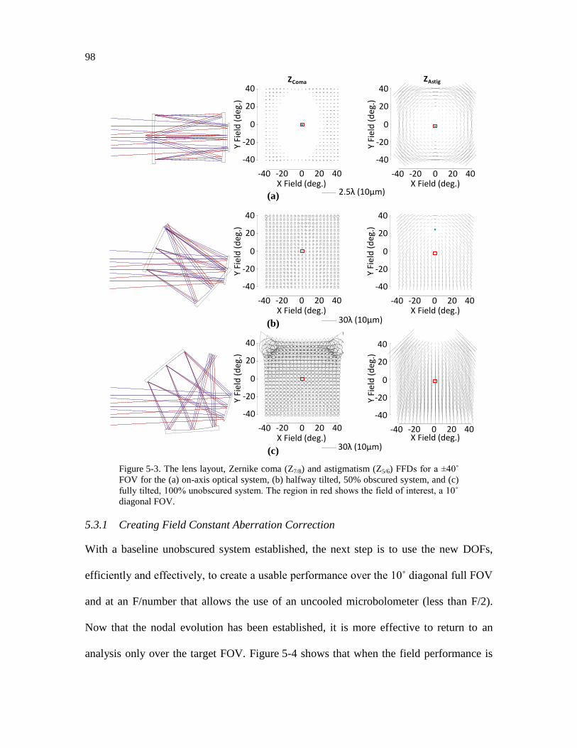
98
(a)
(b)
(c)
14:37:35
Zernike Polynomial KHF 08-Jun-11
25.40 MM
14:37:34
Zernike Polynomial
KHF 08-Jun-11
FRINGE ZERNIKE PAIR Z5 AND Z6
vs
FIELD ANGLE IN OBJECT SPACE
Minimum = 0.41957e-5
Maximum = 2.8641
Average = 0.87527
Std Dev = 0.68384
2.5waves (10000.0 nm)
-40 -20 0 20 40
X Field Angle in Object Space - degrees
-40
-20
0
20
40
Y Field Angle in Object Space - degrees
14:37:35
Zernike Polynomial
KHF 08-Jun-11
FRINGE ZERNIKE PAIR Z7 AND Z8
vs
FIELD ANGLE IN OBJECT SPACE
Minimum = 0.21166e-5
Maximum = 0.14889
Average = 0.076407
Std Dev = 0.049123
2.5waves (10000.0 nm)
-40 -20 0 20 40
X Field Angle in Object Space - degrees
-40
-20
0
20
40
Y Field Angle in Object Space - degrees
ZAstigZComa
14:04:21
Zernike Polynomial
KHF 08-Jun-11
FRINGE ZERNIKE PAIR Z5 AND Z6
vs
FIELD ANGLE IN OBJECT SPACE
Minimum = 0.22109
Maximum = 8.4653
Average = 3.9119
Std Dev = 1.4341
30waves (10000.0 nm)
-40 -20 0 20 40
X Field Angle in Object Space - degrees
-40
-20
0
20
40
Y Field Angle in Object Space - degrees
2.5λ (10µm)
14:05:06
Zernike Polynomial KHF 08-Jun-11
25.40 MM
14:05:06
Zernike Polynomial
KHF 08-Jun-11
FRINGE ZERNIKE PAIR Z5 AND Z6
vs
FIELD ANGLE IN OBJECT SPACE
Minimum = 0.004978
Maximum = 16.328
Average = 9.2986
Std Dev = 3.0961
30waves (10000.0 nm)
-40 -20 0 20 40
X Field Angle in Object Space - degrees
-40
-20
0
20
40
Y Field Angle in Object Space - degrees
14:05:06
Zernike Polynomial
KHF 08-Jun-11
FRINGE ZERNIKE PAIR Z7 AND Z8
vs
FIELD ANGLE IN OBJECT SPACE
Minimum = 3.7002
Maximum = 7.1567
Average = 4.4879
Std Dev = 0.59061
30waves (10000.0 nm)
-40 -20 0 20 40
X Field Angle in Object Space - degrees
-40
-20
0
20
40
Y Field Angle in Object Space - degrees
14:04:21
Zernike Polynomial
KHF 08-Jun-11
FRINGE ZERNIKE PAIR Z5 AND Z6
vs
FIELD ANGLE IN OBJECT SPACE
Minimum = 0.22109
Maximum = 8.4653
Average = 3.9119
Std Dev = 1.4341
30waves (10000.0 nm)
-40 -20 0 20 40
X Field Angle in Object Space - degrees
-40
-20
0
20
40
Y Field Angle in Object Space - degrees
30λ (10µm)
14:06:27
Zernike Polynomial KHF 08-Jun-11
25.40 MM
14:06:26
Zernike Polynomial
KHF 08-Jun-11
FRINGE ZERNIKE PAIR Z5 AND Z6
vs
FIELD ANGLE IN OBJECT SPACE
Minimum = 3.1297
Maximum = 85.517
Average = 29.836
Std Dev = 9.5017
30waves (10000.0 nm)
-40 -20 0 20 40
X Field Angle in Object Space - degrees
-40
-20
0
20
40Y Field Angle in Object Space - degrees
14:06:27
Zernike Polynomial
KHF 08-Jun-11
FRINGE ZERNIKE PAIR Z7 AND Z8
vs
FIELD ANGLE IN OBJECT SPACE
Minimum = 7.0185
Maximum = 53.123
Average = 11.697
Std Dev = 5.3486
30waves (10000.0 nm)
-40 -20 0 20 40
X Field Angle in Object Space - degrees
-40
-20
0
20
40
Y Field Angle in Object Space - degrees
14:04:21
Zernike Polynomial
KHF 08-Jun-11
FRINGE ZERNIKE PAIR Z5 AND Z6
vs
FIELD ANGLE IN OBJECT SPACE
Minimum = 0.22109
Maximum = 8.4653
Average = 3.9119
Std Dev = 1.4341
30waves (10000.0 nm)
-40 -20 0 20 40
X Field Angle in Object Space - degrees
-40
-20
0
20
40
Y Field Angle in Object Space - degrees
30λ (10µm)
40
20
0
-40
-20
-40 -20 0 4020
(a)
(b)
(c)
14:37:35
Zernike Polynomial KHF 08-Jun-11
25.40 MM
14:37:34
Zernike Polynomial
KHF 08-Jun-11
FRINGE ZERNIKE PAIR Z5 AND Z6
vs
FIELD ANGLE IN OBJECT SPACE
Minimum = 0.41957e-5
Maximum = 2.8641
Average = 0.87527
Std Dev = 0.68384
2.5waves (10000.0 nm)
-40 -20 0 20 40
X Field Angle in Object Space - degrees
-40
-20
0
20
40
Y Field Angle in Object Space - degrees
14:37:35
Zernike Polynomial
KHF 08-Jun-11
FRINGE ZERNIKE PAIR Z7 AND Z8
vs
FIELD ANGLE IN OBJECT SPACE
Minimum = 0.21166e-5
Maximum = 0.14889
Average = 0.076407
Std Dev = 0.049123
2.5waves (10000.0 nm)
-40 -20 0 20 40
X Field Angle in Object Space - degrees
-40
-20
0
20
40
Y Field Angle in Object Space - degrees
ZAstigZComa
14:04:21
Zernike Polynomial
KHF 08-Jun-11
FRINGE ZERNIKE PAIR Z5 AND Z6
vs
FIELD ANGLE IN OBJECT SPACE
Minimum = 0.22109
Maximum = 8.4653
Average = 3.9119
Std Dev = 1.4341
30waves (10000.0 nm)
-40 -20 0 20 40
X Field Angle in Object Space - degrees
-40
-20
0
20
40
Y Field Angle in Object Space - degrees
2.5λ (10µm)
14:05:06
Zernike Polynomial KHF 08-Jun-11
25.40 MM
14:05:06
Zernike Polynomial
KHF 08-Jun-11
FRINGE ZERNIKE PAIR Z5 AND Z6
vs
FIELD ANGLE IN OBJECT SPACE
Minimum = 0.004978
Maximum = 16.328
Average = 9.2986
Std Dev = 3.0961
30waves (10000.0 nm)
-40 -20 0 20 40
X Field Angle in Object Space - degrees
-40
-20
0
20
40
Y Field Angle in Object Space - degrees
14:05:06
Zernike Polynomial
KHF 08-Jun-11
FRINGE ZERNIKE PAIR Z7 AND Z8
vs
FIELD ANGLE IN OBJECT SPACE
Minimum = 3.7002
Maximum = 7.1567
Average = 4.4879
Std Dev = 0.59061
30waves (10000.0 nm)
-40 -20 0 20 40
X Field Angle in Object Space - degrees
-40
-20
0
20
40
Y Field Angle in Object Space - degrees
14:04:21
Zernike Polynomial
KHF 08-Jun-11
FRINGE ZERNIKE PAIR Z5 AND Z6
vs
FIELD ANGLE IN OBJECT SPACE
Minimum = 0.22109
Maximum = 8.4653
Average = 3.9119
Std Dev = 1.4341
30waves (10000.0 nm)
-40 -20 0 20 40
X Field Angle in Object Space - degrees
-40
-20
0
20
40
Y Field Angle in Object Space - degrees
30λ (10µm)
14:06:27
Zernike Polynomial KHF 08-Jun-11
25.40 MM
14:06:26
Zernike Polynomial
KHF 08-Jun-11
FRINGE ZERNIKE PAIR Z5 AND Z6
vs
FIELD ANGLE IN OBJECT SPACE
Minimum = 3.1297
Maximum = 85.517
Average = 29.836
Std Dev = 9.5017
30waves (10000.0 nm)
-40 -20 0 20 40
X Field Angle in Object Space - degrees
-40
-20
0
20
40
Y Field Angle in Object Space - degrees
14:06:27
Zernike Polynomial
KHF 08-Jun-11
FRINGE ZERNIKE PAIR Z7 AND Z8
vs
FIELD ANGLE IN OBJECT SPACE
Minimum = 7.0185
Maximum = 53.123
Average = 11.697
Std Dev = 5.3486
30waves (10000.0 nm)
-40 -20 0 20 40
X Field Angle in Object Space - degrees
-40
-20
0
20
40
Y Field Angle in Object Space - degrees
14:04:21
Zernike Polynomial
KHF 08-Jun-11
FRINGE ZERNIKE PAIR Z5 AND Z6
vs
FIELD ANGLE IN OBJECT SPACE
Minimum = 0.22109
Maximum = 8.4653
Average = 3.9119
Std Dev = 1.4341
30waves (10000.0 nm)
-40 -20 0 20 40
X Field Angle in Object Space - degrees
-40
-20
0
20
40Y Field Angle in Object Space - degrees
30λ (10µm)
40
20
0
-40
-20
-40 -20 0 4020
40
20
0
-40
-20
-40 -20 0 4020
40
20
0
-40
-20
-40 -20 0 4020
40
20
0
-40
-20
-40 -20 0 4020
40
20
0
-40
-20
-40 -20 0 4020
(a)
(b)
(c)
14:37:35
Zernike Polynomial KHF 08-Jun-11
25.40 MM
14:37:34
Zernike Polynomial
KHF 08-Jun-11
FRINGE ZERNIKE PAIR Z5 AND Z6
vs
FIELD ANGLE IN OBJECT SPACE
Minimum = 0.41957e-5
Maximum = 2.8641
Average = 0.87527
Std Dev = 0.68384
2.5waves (10000.0 nm)
-40 -20 0 20 40
X Field Angle in Object Space - degrees
-40
-20
0
20
40
Y Field Angle in Object Space - degrees
14:37:35
Zernike Polynomial
KHF 08-Jun-11
FRINGE ZERNIKE PAIR Z7 AND Z8
vs
FIELD ANGLE IN OBJECT SPACE
Minimum = 0.21166e-5
Maximum = 0.14889
Average = 0.076407
Std Dev = 0.049123
2.5waves (10000.0 nm)
-40 -20 0 20 40
X Field Angle in Object Space - degrees
-40
-20
0
20
40
Y Field Angle in Object Space - degrees
ZAstigZComa
14:04:21
Zernike Polynomial
KHF 08-Jun-11
FRINGE ZERNIKE PAIR Z5 AND Z6
vs
FIELD ANGLE IN OBJECT SPACE
Minimum = 0.22109
Maximum = 8.4653
Average = 3.9119
Std Dev = 1.4341
30waves (10000.0 nm)
-40 -20 0 20 40
X Field Angle in Object Space - degrees
-40
-20
0
20
40
Y Field Angle in Object Space - degrees
2.5λ (10µm)
14:05:06
Zernike Polynomial KHF 08-Jun-11
25.40 MM
14:05:06
Zernike Polynomial
KHF 08-Jun-11
FRINGE ZERNIKE PAIR Z5 AND Z6
vs
FIELD ANGLE IN OBJECT SPACE
Minimum = 0.004978
Maximum = 16.328
Average = 9.2986
Std Dev = 3.0961
30waves (10000.0 nm)
-40 -20 0 20 40
X Field Angle in Object Space - degrees
-40
-20
0
20
40
Y Field Angle in Object Space - degrees
14:05:06
Zernike Polynomial
KHF 08-Jun-11
FRINGE ZERNIKE PAIR Z7 AND Z8
vs
FIELD ANGLE IN OBJECT SPACE
Minimum = 3.7002
Maximum = 7.1567
Average = 4.4879
Std Dev = 0.59061
30waves (10000.0 nm)
-40 -20 0 20 40
X Field Angle in Object Space - degrees
-40
-20
0
20
40
Y Field Angle in Object Space - degrees
14:04:21
Zernike Polynomial
KHF 08-Jun-11
FRINGE ZERNIKE PAIR Z5 AND Z6
vs
FIELD ANGLE IN OBJECT SPACE
Minimum = 0.22109
Maximum = 8.4653
Average = 3.9119
Std Dev = 1.4341
30waves (10000.0 nm)
-40 -20 0 20 40
X Field Angle in Object Space - degrees
-40
-20
0
20
40
Y Field Angle in Object Space - degrees
30λ (10µm)
14:06:27
Zernike Polynomial KHF 08-Jun-11
25.40 MM
14:06:26
Zernike Polynomial
KHF 08-Jun-11
FRINGE ZERNIKE PAIR Z5 AND Z6
vs
FIELD ANGLE IN OBJECT SPACE
Minimum = 3.1297
Maximum = 85.517
Average = 29.836
Std Dev = 9.5017
30waves (10000.0 nm)
-40 -20 0 20 40
X Field Angle in Object Space - degrees
-40
-20
0
20
40
Y Field Angle in Object Space - degrees
14:06:27
Zernike Polynomial
KHF 08-Jun-11
FRINGE ZERNIKE PAIR Z7 AND Z8
vs
FIELD ANGLE IN OBJECT SPACE
Minimum = 7.0185
Maximum = 53.123
Average = 11.697
Std Dev = 5.3486
30waves (10000.0 nm)
-40 -20 0 20 40
X Field Angle in Object Space - degrees
-40
-20
0
20
40
Y Field Angle in Object Space - degrees
14:04:21
Zernike Polynomial
KHF 08-Jun-11
FRINGE ZERNIKE PAIR Z5 AND Z6
vs
FIELD ANGLE IN OBJECT SPACE
Minimum = 0.22109
Maximum = 8.4653
Average = 3.9119
Std Dev = 1.4341
30waves (10000.0 nm)
-40 -20 0 20 40
X Field Angle in Object Space - degrees
-40
-20
0
20
40
Y Field Angle in Object Space - degrees
30λ (10µm)
YFi
eld
(d
eg.)
X Field (deg.)
YFi
eld
(d
eg.)
X Field (deg.)
YFi
eld
(d
eg.)
X Field (deg.)
YFi
eld
(d
eg.)
X Field (deg.)
YFi
eld
(d
eg.)
X Field (deg.)
YFi
eld
(d
eg.)
X Field (deg.)
2.5λ (10µm)
30λ (10µm)
30λ (10µm)
Figure 5-3. The lens layout, Zernike coma (Z7/8) and astigmatism (Z5/6) FFDs for a ±40˚
FOV for the (a) on-axis optical system, (b) halfway tilted, 50% obscured system, and (c)
fully tilted, 100% unobscured system. The region in red shows the field of interest, a 10˚
diagonal FOV.
5.3.1 Creating Field Constant Aberration Correction
With a baseline unobscured system established, the next step is to use the new DOFs,
efficiently and effectively, to create a usable performance over the 10˚ diagonal full FOV
and at an F/number that allows the use of an uncooled microbolometer (less than F/2).
Now that the nodal evolution has been established, it is more effective to return to an
analysis only over the target FOV. Figure 5-4 shows that when the field performance is
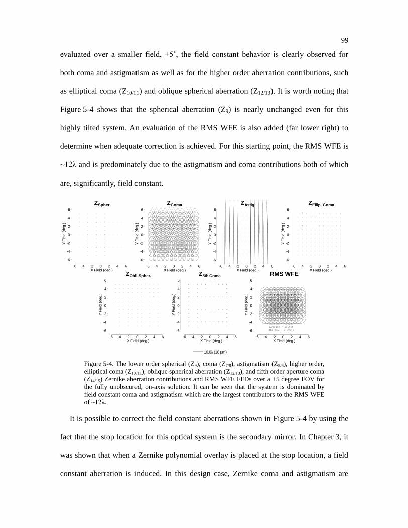
99
evaluated over a smaller field, ±5˚, the field constant behavior is clearly observed for
both coma and astigmatism as well as for the higher order aberration contributions, such
as elliptical coma (Z10/11) and oblique spherical aberration (Z12/13). It is worth noting that
Figure 5-4 shows that the spherical aberration (Z9) is nearly unchanged even for this
highly tilted system. An evaluation of the RMS WFE is also added (far lower right) to
determine when adequate correction is achieved. For this starting point, the RMS WFE is
~12λ and is predominately due to the astigmatism and coma contributions both of which
are, significantly, field constant.
13:52:59
Zernike Polynomial
KHF 23-Sep-13
FRINGE ZERNIKE PAIR Z5 AND Z6
vs
FIELD ANGLE IN OBJECT SPACE
Minimum = 31.614
Maximum = 34.206
Average = 32.948
Std Dev = 0.74182
10waves (10000.0 nm)
-6 -4 -2 0 2 4 6
X Field Angle in Object Space - degrees
-6
-4
-2
0
2
4
6Y Field Angle in Object Space - degrees
13:52:59
Zernike Polynomial
KHF 23-Sep-13
FRINGE ZERNIKE PAIR Z7 AND Z8
vs
FIELD ANGLE IN OBJECT SPACE
Minimum = 10.975
Maximum = 12.996
Average = 11.927
Std Dev = 0.62792
10waves (10000.0 nm)
-6 -4 -2 0 2 4 6
X Field Angle in Object Space - degrees
-6
-4
-2
0
2
4
6
Y Field Angle in Object Space - degrees
13:53:00
Zernike Polynomial
KHF 23-Sep-13
FRINGE ZERNIKE COEFFICIENT Z9
vs
FIELD ANGLE IN OBJECT SPACE
Minimum = -0.2004
Maximum = -0.17296
Average = -0.18392
Std Dev = 0.0080848
10waves (10000.0 nm)
-6 -4 -2 0 2 4 6
X Field Angle in Object Space - degrees
-6
-4
-2
0
2
4
6
Y Field Angle in Object Space - degrees
13:53:00
Zernike Polynomial
KHF 23-Sep-13
FRINGE ZERNIKE PAIR Z10 AND Z11
vs
FIELD ANGLE IN OBJECT SPACE
Minimum = 0.92293
Maximum = 1.3468
Average = 1.123
Std Dev = 0.13169
10waves (10000.0 nm)
-6 -4 -2 0 2 4 6
X Field Angle in Object Space - degrees
-6
-4
-2
0
2
4
6
Y Field Angle in Object Space - degrees
13:53:00
Zernike Polynomial
KHF 23-Sep-13
FRINGE ZERNIKE PAIR Z12 AND Z13
vs
FIELD ANGLE IN OBJECT SPACE
Minimum = 0.26485
Maximum = 0.53057
Average = 0.3919
Std Dev = 0.080087
10waves (10000.0 nm)
-6 -4 -2 0 2 4 6
X Field Angle in Object Space - degrees
-6
-4
-2
0
2
4
6
Y Field Angle in Object Space - degrees
13:53:00
Zernike Polynomial
KHF 23-Sep-13
FRINGE ZERNIKE PAIR Z14 AND Z15
vs
FIELD ANGLE IN OBJECT SPACE
Minimum = 0.17107
Maximum = 0.22424
Average = 0.19594
Std Dev = 0.016572
10waves (10000.0 nm)
-6 -4 -2 0 2 4 6
X Field Angle in Object Space - degrees
-6
-4
-2
0
2
4
6
Y Field Angle in Object Space - degrees
13:53:01
Zernike Polynomial
KHF 23-Sep-13
RMS WAVEFRONT ERROR
vs
FIELD ANGLE IN OBJECT SPACE
Minimum = 11.294
Maximum = 12.351
Average = 11.905
Std Dev = 0.29646
10waves (10000.0 nm)
-6 -4 -2 0 2 4 6
X Field Angle in Object Space - degrees
-6
-4
-2
0
2
4
6
Y Field Angle in Object Space - degrees
6 4 2 0 642- - -X Field (deg.)
6-
4-
2-
0
2
4
6
Y F
ield
(deg.)
6 4 2 0 642- - -X Field (deg.)
6-
4-
2-
0
2
4
6
Y F
ield
(deg.)
6 4 2 0 642- - -X Field (deg.)
6-
4-
2-
0
2
4
6Y
Fie
ld (
deg.)
6 4 2 0 642- - -X Field (deg.)
6-
4-
2-
0
2
4
6
Y F
ield
(deg.)
6 4 2 0 642- - -X Field (deg.)
6-
4-
2-
0
2
4
6
Y F
ield
(deg.)
6 4 2 0 642- - -X Field (deg.)
6-
4-
2-
0
2
4
6
Y F
ield
(deg.)
6 4 2 0 642- - -X Field (deg.)
6-
4-
2-
0
2
4
6
Y F
ield
(deg.)
ZEllip. Coma
ZObl .Spher. RMS WFE
ZAstigZComaZSpher
Z5th Coma
14:37:41
Zernike Polynomial
KHF 23-Sep-13
FRINGE ZERNIKE COEFFICIENT Z9
vs
FIELD ANGLE IN OBJECT SPACE
Minimum = -0.015258
Maximum = 0.012736
Average = 0.00036325
Std Dev = 0.0086811
0.25waves (10000.0 nm)
-6 -4 -2 0 2 4 6
X Field Angle in Object Space - degrees
-6
-4
-2
0
2
4
6
Y Field Angle in Object Space - degrees
10.0λ (10 µm)
13:53:01
Zernike Polynomial
KHF 23-Sep-13
RMS WAVEFRONT ERROR
vs
FIELD ANGLE IN OBJECT SPACE
Minimum = 11.294
Maximum = 12.351
Average = 11.905
Std Dev = 0.29646
10waves (10000.0 nm)
-6 -4 -2 0 2 4 6
X Field Angle in Object Space - degrees
-6
-4
-2
0
2
4
6
Y Field Angle in Object Space - degrees
Figure 5-4. The lower order spherical (Z9), coma (Z7/8), astigmatism (Z5/6), higher order,
elliptical coma (Z10/11), oblique spherical aberration (Z12/13), and fifth order aperture coma
(Z14/15) Zernike aberration contributions and RMS WFE FFDs over a ±5 degree FOV for
the fully unobscured, on-axis solution. It can be seen that the system is dominated by
field constant coma and astigmatism which are the largest contributors to the RMS WFE
of ~12λ.
It is possible to correct the field constant aberrations shown in Figure 5-4 by using the
fact that the stop location for this optical system is the secondary mirror. In Chapter 3, it
was shown that when a Zernike polynomial overlay is placed at the stop location, a field
constant aberration is induced. In this design case, Zernike coma and astigmatism are
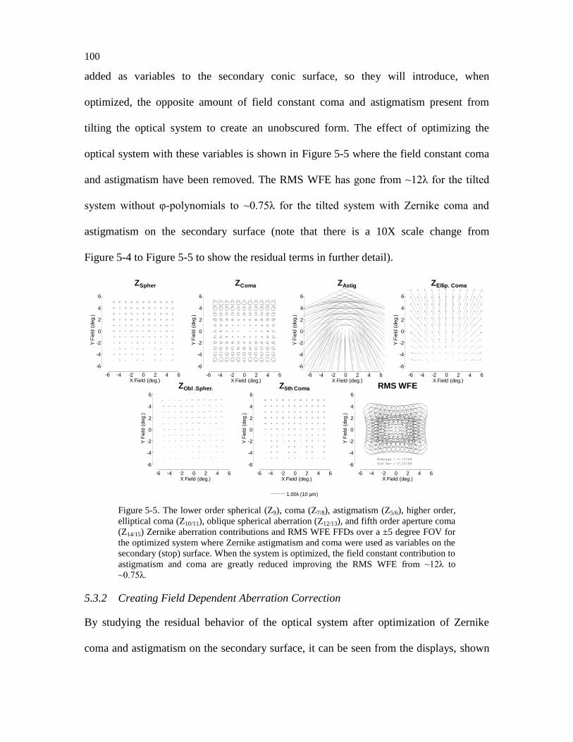
100
added as variables to the secondary conic surface, so they will introduce, when
optimized, the opposite amount of field constant coma and astigmatism present from
tilting the optical system to create an unobscured form. The effect of optimizing the
optical system with these variables is shown in Figure 5-5 where the field constant coma
and astigmatism have been removed. The RMS WFE has gone from ~12λ for the tilted
system without φ-polynomials to ~0.75λ for the tilted system with Zernike coma and
astigmatism on the secondary surface (note that there is a 10X scale change from
Figure 5-4 to Figure 5-5 to show the residual terms in further detail).
13:57:21
Zernike Polynomial
KHF 23-Sep-13
FRINGE ZERNIKE PAIR Z5 AND Z6
vs
FIELD ANGLE IN OBJECT SPACE
Minimum = 0.054353
Maximum = 5.0395
Average = 2.7771
Std Dev = 1.0497
1waves (10000.0 nm)
-6 -4 -2 0 2 4 6
X Field Angle in Object Space - degrees
-6
-4
-2
0
2
4
6
Y Field Angle in Object Space - degrees
13:57:21
Zernike Polynomial
KHF 23-Sep-13
FRINGE ZERNIKE PAIR Z7 AND Z8
vs
FIELD ANGLE IN OBJECT SPACE
Minimum = 0.0052108
Maximum = 0.47304
Average = 0.25737
Std Dev = 0.11196
1waves (10000.0 nm)
-6 -4 -2 0 2 4 6
X Field Angle in Object Space - degrees
-6
-4
-2
0
2
4
6
Y Field Angle in Object Space - degrees
13:57:21
Zernike Polynomial
KHF 23-Sep-13
FRINGE ZERNIKE COEFFICIENT Z9
vs
FIELD ANGLE IN OBJECT SPACE
Minimum = 0.031014
Maximum = 0.10608
Average = 0.067278
Std Dev = 0.023332
1waves (10000.0 nm)
-6 -4 -2 0 2 4 6
X Field Angle in Object Space - degrees
-6
-4
-2
0
2
4
6
Y Field Angle in Object Space - degrees
13:57:22
Zernike Polynomial
KHF 23-Sep-13
FRINGE ZERNIKE PAIR Z10 AND Z11
vs
FIELD ANGLE IN OBJECT SPACE
Minimum = 0.027263
Maximum = 1.0754
Average = 0.57087
Std Dev = 0.26785
1waves (10000.0 nm)
-6 -4 -2 0 2 4 6
X Field Angle in Object Space - degrees
-6
-4
-2
0
2
4
6
Y Field Angle in Object Space - degrees
13:57:22
Zernike Polynomial
KHF 23-Sep-13
FRINGE ZERNIKE PAIR Z12 AND Z13
vs
FIELD ANGLE IN OBJECT SPACE
Minimum = 0.052021
Maximum = 0.18089
Average = 0.11437
Std Dev = 0.038553
1waves (10000.0 nm)
-6 -4 -2 0 2 4 6
X Field Angle in Object Space - degrees
-6
-4
-2
0
2
4
6
Y Field Angle in Object Space - degrees
13:57:22
Zernike Polynomial
KHF 23-Sep-13
FRINGE ZERNIKE PAIR Z14 AND Z15
vs
FIELD ANGLE IN OBJECT SPACE
Minimum = 0.063068
Maximum = 0.095524
Average = 0.078182
Std Dev = 0.010147
1waves (10000.0 nm)
-6 -4 -2 0 2 4 6
X Field Angle in Object Space - degrees
-6
-4
-2
0
2
4
6
Y Field Angle in Object Space - degrees
13:57:22
Zernike Polynomial
KHF 23-Sep-13
RMS WAVEFRONT ERROR
vs
FIELD ANGLE IN OBJECT SPACE
Minimum = 0.13731
Maximum = 1.2474
Average = 0.71749
Std Dev = 0.25169
1waves (10000.0 nm)
-6 -4 -2 0 2 4 6
X Field Angle in Object Space - degrees
-6
-4
-2
0
2
4
6
Y Field Angle in Object Space - degrees
6 4 2 0 642- - -X Field (deg.)
6-
4-
2-
0
2
4
6
Y F
ield
(deg.)
6 4 2 0 642- - -X Field (deg.)
6-
4-
2-
0
2
4
6
Y F
ield
(deg.)
6 4 2 0 642- - -X Field (deg.)
Y F
ield
(deg.)
6
4
2
0
2-
4-
6-
6 4 2 0 642- - -X Field (deg.)
6-
4-
2-
0
2
4
6
Y F
ield
(deg.)
6 4 2 0 642- - -X Field (deg.)
6-
4-
2-
0
2
4
6
Y F
ield
(deg.)
6 4 2 0 642- - -X Field (deg.)
6-
4-
2-
0
2
4
6
Y F
ield
(deg.)
6 4 2 0 642- - -X Field (deg.)
6-
4-
2-
0
2
4
6
Y F
ield
(deg.)
ZEllip. Coma
ZObl .Spher. RMS WFE
ZAstigZComaZSpher
Z5th Coma
14:37:41
Zernike Polynomial
KHF 23-Sep-13
FRINGE ZERNIKE COEFFICIENT Z9
vs
FIELD ANGLE IN OBJECT SPACE
Minimum = -0.015258
Maximum = 0.012736
Average = 0.00036325
Std Dev = 0.0086811
0.25waves (10000.0 nm)
-6 -4 -2 0 2 4 6
X Field Angle in Object Space - degrees
-6
-4
-2
0
2
4
6
Y Field Angle in Object Space - degrees
1.00λ (10 µm)
13:57:22
Zernike Polynomial
KHF 23-Sep-13
RMS WAVEFRONT ERROR
vs
FIELD ANGLE IN OBJECT SPACE
Minimum = 0.13731
Maximum = 1.2474
Average = 0.71749
Std Dev = 0.25169
1waves (10000.0 nm)
-6 -4 -2 0 2 4 6
X Field Angle in Object Space - degrees
-6
-4
-2
0
2
4
6
Y Field Angle in Object Space - degrees
Figure 5-5. The lower order spherical (Z9), coma (Z7/8), astigmatism (Z5/6), higher order,
elliptical coma (Z10/11), oblique spherical aberration (Z12/13), and fifth order aperture coma
(Z14/15) Zernike aberration contributions and RMS WFE FFDs over a ±5 degree FOV for
the optimized system where Zernike astigmatism and coma were used as variables on the
secondary (stop) surface. When the system is optimized, the field constant contribution to
astigmatism and coma are greatly reduced improving the RMS WFE from ~12λ to
~0.75λ.
5.3.2 Creating Field Dependent Aberration Correction
By studying the residual behavior of the optical system after optimization of Zernike
coma and astigmatism on the secondary surface, it can be seen from the displays, shown
101
in Figure 5-5, that the dominant aberration contribution is Zernike astigmatism and it is
the largest contributor to the RMS WFE of ~0.75λ. Moreover, the astigmatism has taken
the form of field linear, field asymmetric astigmatism. In Chapter 3, it was discovered
that a Zernike coma overlay displaced axially away from the stop surface will introduce
field linear, field asymmetric astigmatism as well as field linear, field curvature. Using
this result, Zernike coma is placed on an optical surface away from the stop location, that
is, the primary or tertiary surface, and optimized to reduce (and in some cases eliminate)
the residual field linear, field asymmetric astigmatism. However, in order to effectively
use this added variable, the tilt angle of the focal plane must also be varied to compensate
the induced field linear, field curvature component also introduced by the Zernike coma
overlay.
Since both the primary and tertiary surfaces lie away from the stop surface, a Zernike
coma overlay can be placed on either surface. If the equation for the generated field
linear, field asymmetric astigmatism from a Zernike coma overlay away from the stop is
investigated, Eq. (3.25), it can be seen that the magnitude of the aberration depends
linearly on the ratio of the chief to marginal ray on the optical surface. For the current
configuration, the ratio at the primary surface is roughly 0.170 whereas the ratio is 0.086
on the tertiary surface. Based on this first order analysis, it appears that the primary
surface will be a much more effective variable for removing the residual field linear, field
asymmetric astigmatism since less comatic departure will be required to create the
equivalent induced astigmatic aberration.
The effectiveness of the Zernike coma overlay on the primary mirror surface is
demonstrated in Figure 5-6 where the relevant aberration contributions after optimization
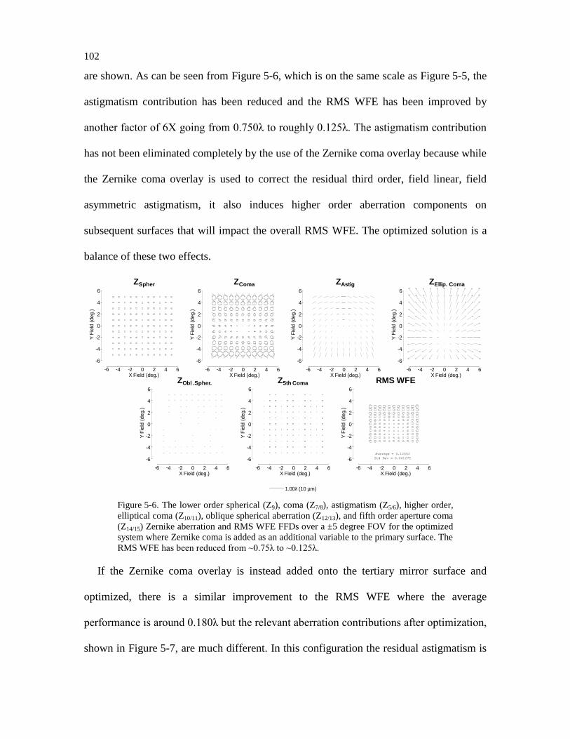
102
are shown. As can be seen from Figure 5-6, which is on the same scale as Figure 5-5, the
astigmatism contribution has been reduced and the RMS WFE has been improved by
another factor of 6X going from 0.750λ to roughly 0.125λ. The astigmatism contribution
has not been eliminated completely by the use of the Zernike coma overlay because while
the Zernike coma overlay is used to correct the residual third order, field linear, field
asymmetric astigmatism, it also induces higher order aberration components on
subsequent surfaces that will impact the overall RMS WFE. The optimized solution is a
balance of these two effects.
13:58:22
Zernike Polynomial
KHF 23-Sep-13
FRINGE ZERNIKE PAIR Z5 AND Z6
vs
FIELD ANGLE IN OBJECT SPACE
Minimum = 0.0073
Maximum = 0.4213
Average = 0.21883
Std Dev = 0.091257
1waves (10000.0 nm)
-6 -4 -2 0 2 4 6
X Field Angle in Object Space - degrees
-6
-4
-2
0
2
4
6Y Field Angle in Object Space - degrees
13:58:22
Zernike Polynomial
KHF 23-Sep-13
FRINGE ZERNIKE PAIR Z7 AND Z8
vs
FIELD ANGLE IN OBJECT SPACE
Minimum = 0.033723
Maximum = 0.56428
Average = 0.30152
Std Dev = 0.12926
1waves (10000.0 nm)
-6 -4 -2 0 2 4 6
X Field Angle in Object Space - degrees
-6
-4
-2
0
2
4
6
Y Field Angle in Object Space - degrees
13:58:22
Zernike Polynomial
KHF 23-Sep-13
FRINGE ZERNIKE COEFFICIENT Z9
vs
FIELD ANGLE IN OBJECT SPACE
Minimum = 0.072859
Maximum = 0.086048
Average = 0.082145
Std Dev = 0.0038394
1waves (10000.0 nm)
-6 -4 -2 0 2 4 6
X Field Angle in Object Space - degrees
-6
-4
-2
0
2
4
6
Y Field Angle in Object Space - degrees
13:58:23
Zernike Polynomial
KHF 23-Sep-13
FRINGE ZERNIKE PAIR Z10 AND Z11
vs
FIELD ANGLE IN OBJECT SPACE
Minimum = 0.0020488
Maximum = 0.80295
Average = 0.4397
Std Dev = 0.17715
1waves (10000.0 nm)
-6 -4 -2 0 2 4 6
X Field Angle in Object Space - degrees
-6
-4
-2
0
2
4
6
Y Field Angle in Object Space - degrees
13:58:23
Zernike Polynomial
KHF 23-Sep-13
FRINGE ZERNIKE PAIR Z12 AND Z13
vs
FIELD ANGLE IN OBJECT SPACE
Minimum = 0.0048849
Maximum = 0.053164
Average = 0.028583
Std Dev = 0.014843
1waves (10000.0 nm)
-6 -4 -2 0 2 4 6
X Field Angle in Object Space - degrees
-6
-4
-2
0
2
4
6
Y Field Angle in Object Space - degrees
13:58:23
Zernike Polynomial
KHF 23-Sep-13
FRINGE ZERNIKE PAIR Z14 AND Z15
vs
FIELD ANGLE IN OBJECT SPACE
Minimum = 0.036374
Maximum = 0.046397
Average = 0.042713
Std Dev = 0.0031971
1waves (10000.0 nm)
-6 -4 -2 0 2 4 6
X Field Angle in Object Space - degrees
-6
-4
-2
0
2
4
6
Y Field Angle in Object Space - degrees
13:58:24
Zernike Polynomial
KHF 23-Sep-13
RMS WAVEFRONT ERROR
vs
FIELD ANGLE IN OBJECT SPACE
Minimum = 0.04427
Maximum = 0.21659
Average = 0.12552
Std Dev = 0.041275
1waves (10000.0 nm)
-6 -4 -2 0 2 4 6
X Field Angle in Object Space - degrees
-6
-4
-2
0
2
4
6
Y Field Angle in Object Space - degrees
6 4 2 0 642- - -X Field (deg.)
6-
4-
2-
0
2
4
6
YF
ield
(deg.)
6 4 2 0 642- - -X Field (deg.)
6-
4-
2-
0
2
4
6
YF
ield
(deg.)
6 4 2 0 642- - -X Field (deg.)
6-
4-
2-
0
2
4
6Y
Fie
ld (
deg.)
6 4 2 0 642- - -X Field (deg.)
6-
4-
2-
0
2
4
6
YF
ield
(deg.)
6 4 2 0 642- - -X Field (deg.)
6-
4-
2-
0
2
4
6
YF
ield
(deg.)
6 4 2 0 642- - -X Field (deg.)
6-
4-
2-
0
2
4
6
YF
ield
(deg.)
6 4 2 0 642- - -X Field (deg.)
6-
4-
2-
0
2
4
6
YF
ield
(deg.)
ZEllip. Coma
ZObl .Spher. RMS WFE
ZAstigZComaZSpher
Z5th Coma
14:37:41
Zernike Polynomial
KHF 23-Sep-13
FRINGE ZERNIKE COEFFICIENT Z9
vs
FIELD ANGLE IN OBJECT SPACE
Minimum = -0.015258
Maximum = 0.012736
Average = 0.00036325
Std Dev = 0.0086811
0.25waves (10000.0 nm)
-6 -4 -2 0 2 4 6
X Field Angle in Object Space - degrees
-6
-4
-2
0
2
4
6
Y Field Angle in Object Space - degrees
1.00λ (10 µm)
13:58:24
Zernike Polynomial
KHF 23-Sep-13
RMS WAVEFRONT ERROR
vs
FIELD ANGLE IN OBJECT SPACE
Minimum = 0.04427
Maximum = 0.21659
Average = 0.12552
Std Dev = 0.041275
1waves (10000.0 nm)
-6 -4 -2 0 2 4 6
X Field Angle in Object Space - degrees
-6
-4
-2
0
2
4
6
Y Field Angle in Object Space - degrees
Figure 5-6. The lower order spherical (Z9), coma (Z7/8), astigmatism (Z5/6), higher order,
elliptical coma (Z10/11), oblique spherical aberration (Z12/13), and fifth order aperture coma
(Z14/15) Zernike aberration and RMS WFE FFDs over a ±5 degree FOV for the optimized
system where Zernike coma is added as an additional variable to the primary surface. The
RMS WFE has been reduced from ~0.75λ to ~0.125λ.
If the Zernike coma overlay is instead added onto the tertiary mirror surface and
optimized, there is a similar improvement to the RMS WFE where the average
performance is around 0.180λ but the relevant aberration contributions after optimization,
shown in Figure 5-7, are much different. In this configuration the residual astigmatism is
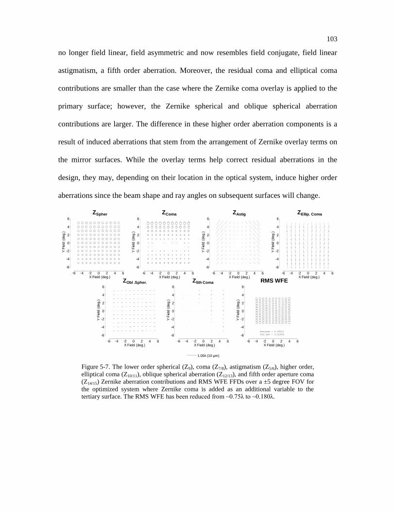
103
no longer field linear, field asymmetric and now resembles field conjugate, field linear
astigmatism, a fifth order aberration. Moreover, the residual coma and elliptical coma
contributions are smaller than the case where the Zernike coma overlay is applied to the
primary surface; however, the Zernike spherical and oblique spherical aberration
contributions are larger. The difference in these higher order aberration components is a
result of induced aberrations that stem from the arrangement of Zernike overlay terms on
the mirror surfaces. While the overlay terms help correct residual aberrations in the
design, they may, depending on their location in the optical system, induce higher order
aberrations since the beam shape and ray angles on subsequent surfaces will change. 13:59:50
Zernike Polynomial
KHF 23-Sep-13
FRINGE ZERNIKE PAIR Z5 AND Z6
vs
FIELD ANGLE IN OBJECT SPACE
Minimum = 0.0057161
Maximum = 0.68543
Average = 0.28603
Std Dev = 0.1636
1waves (10000.0 nm)
-6 -4 -2 0 2 4 6
X Field Angle in Object Space - degrees
-6
-4
-2
0
2
4
6
Y Field Angle in Object Space - degrees
13:59:51
Zernike Polynomial
KHF 23-Sep-13
FRINGE ZERNIKE PAIR Z7 AND Z8
vs
FIELD ANGLE IN OBJECT SPACE
Minimum = 0.013632
Maximum = 0.36969
Average = 0.14397
Std Dev = 0.10007
1waves (10000.0 nm)
-6 -4 -2 0 2 4 6
X Field Angle in Object Space - degrees
-6
-4
-2
0
2
4
6
Y Field Angle in Object Space - degrees
13:59:51
Zernike Polynomial
KHF 23-Sep-13
FRINGE ZERNIKE COEFFICIENT Z9
vs
FIELD ANGLE IN OBJECT SPACE
Minimum = -0.21641
Maximum = -0.14896
Average = -0.18044
Std Dev = 0.020724
1waves (10000.0 nm)
-6 -4 -2 0 2 4 6
X Field Angle in Object Space - degrees
-6
-4
-2
0
2
4
6
Y Field Angle in Object Space - degrees
13:59:51
Zernike Polynomial
KHF 23-Sep-13
FRINGE ZERNIKE PAIR Z10 AND Z11
vs
FIELD ANGLE IN OBJECT SPACE
Minimum = 0.44899
Maximum = 0.5808
Average = 0.52974
Std Dev = 0.036596
1waves (10000.0 nm)
-6 -4 -2 0 2 4 6
X Field Angle in Object Space - degrees
-6
-4
-2
0
2
4
6
Y Field Angle in Object Space - degrees
13:59:51
Zernike Polynomial
KHF 23-Sep-13
FRINGE ZERNIKE PAIR Z12 AND Z13
vs
FIELD ANGLE IN OBJECT SPACE
Minimum = 0.10484
Maximum = 0.14582
Average = 0.12655
Std Dev = 0.012196
1waves (10000.0 nm)
-6 -4 -2 0 2 4 6
X Field Angle in Object Space - degrees
-6
-4
-2
0
2
4
6
Y Field Angle in Object Space - degrees
13:59:51
Zernike Polynomial
KHF 23-Sep-13
FRINGE ZERNIKE PAIR Z14 AND Z15
vs
FIELD ANGLE IN OBJECT SPACE
Minimum = 0.010167
Maximum = 0.023382
Average = 0.016188
Std Dev = 0.0040848
1waves (10000.0 nm)
-6 -4 -2 0 2 4 6
X Field Angle in Object Space - degrees
-6
-4
-2
0
2
4
6
Y Field Angle in Object Space - degrees
13:59:52
Zernike Polynomial
KHF 23-Sep-13
RMS WAVEFRONT ERROR
vs
FIELD ANGLE IN OBJECT SPACE
Minimum = 0.14727
Maximum = 0.21404
Average = 0.18221
Std Dev = 0.01856
1waves (10000.0 nm)
-6 -4 -2 0 2 4 6
X Field Angle in Object Space - degrees
-6
-4
-2
0
2
4
6
Y Field Angle in Object Space - degrees
6 4 2 0 642- - -X Field (deg.)
6-
4-
2-
0
2
4
6
YF
ield
(deg.)
6 4 2 0 642- - -X Field (deg.)
6-
4-
2-
0
2
4
6
YF
ield
(deg.)
6 4 2 0 642- - -X Field (deg.)
6-
4-
2-
0
2
4
6
YF
ield
(deg.)
6 4 2 0 642- - -X Field (deg.)
6-
4-
2-
0
2
4
6
YF
ield
(deg.)
6 4 2 0 642- - -X Field (deg.)
6-
4-
2-
0
2
4
6
YF
ield
(deg.)
6 4 2 0 642- - -X Field (deg.)
6-
4-
2-
0
2
4
6
YF
ield
(deg.)
6 4 2 0 642- - -X Field (deg.)
6-
4-
2-
0
2
4
6
YF
ield
(deg.)
ZEllip. Coma
ZObl .Spher. RMS WFE
ZAstigZComaZSpher
Z5th Coma
14:37:41
Zernike Polynomial
KHF 23-Sep-13
FRINGE ZERNIKE COEFFICIENT Z9
vs
FIELD ANGLE IN OBJECT SPACE
Minimum = -0.015258
Maximum = 0.012736
Average = 0.00036325
Std Dev = 0.0086811
0.25waves (10000.0 nm)
-6 -4 -2 0 2 4 6
X Field Angle in Object Space - degrees
-6
-4
-2
0
2
4
6
Y Field Angle in Object Space - degrees
1.00λ (10 µm)
13:59:52
Zernike Polynomial
KHF 23-Sep-13
RMS WAVEFRONT ERROR
vs
FIELD ANGLE IN OBJECT SPACE
Minimum = 0.14727
Maximum = 0.21404
Average = 0.18221
Std Dev = 0.01856
1waves (10000.0 nm)
-6 -4 -2 0 2 4 6
X Field Angle in Object Space - degrees
-6
-4
-2
0
2
4
6Y Field Angle in Object Space - degrees
Figure 5-7. The lower order spherical (Z9), coma (Z7/8), astigmatism (Z5/6), higher order,
elliptical coma (Z10/11), oblique spherical aberration (Z12/13), and fifth order aperture coma
(Z14/15) Zernike aberration contributions and RMS WFE FFDs over a ±5 degree FOV for
the optimized system where Zernike coma is added as an additional variable to the
tertiary surface. The RMS WFE has been reduced from ~0.75λ to ~0.180λ.
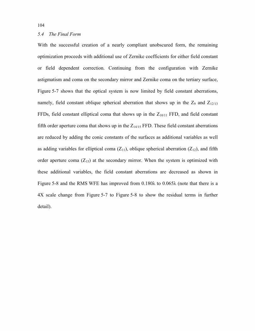
104
5.4 The Final Form
With the successful creation of a nearly compliant unobscured form, the remaining
optimization proceeds with additional use of Zernike coefficients for either field constant
or field dependent correction. Continuing from the configuration with Zernike
astigmatism and coma on the secondary mirror and Zernike coma on the tertiary surface,
Figure 5-7 shows that the optical system is now limited by field constant aberrations,
namely, field constant oblique spherical aberration that shows up in the Z9 and Z12/13
FFDs, field constant elliptical coma that shows up in the Z10/11 FFD, and field constant
fifth order aperture coma that shows up in the Z14/15 FFD. These field constant aberrations
are reduced by adding the conic constants of the surfaces as additional variables as well
as adding variables for elliptical coma (Z11), oblique spherical aberration (Z12), and fifth
order aperture coma (Z15) at the secondary mirror. When the system is optimized with
these additional variables, the field constant aberrations are decreased as shown in
Figure 5-8 and the RMS WFE has improved from 0.180λ to 0.065λ (note that there is a
4X scale change from Figure 5-7 to Figure 5-8 to show the residual terms in further
detail).
105
14:28:48
Zernike Polynomial
KHF 23-Sep-13
FRINGE ZERNIKE PAIR Z5 AND Z6
vs
FIELD ANGLE IN OBJECT SPACE
Minimum = 0.012678
Maximum = 0.50061
Average = 0.27048
Std Dev = 0.11969
0.25waves (10000.0 nm)
-6 -4 -2 0 2 4 6
X Field Angle in Object Space - degrees
-6
-4
-2
0
2
4
6
Y Field Angle in Object Space - degrees
14:28:48
Zernike Polynomial
KHF 23-Sep-13
FRINGE ZERNIKE PAIR Z7 AND Z8
vs
FIELD ANGLE IN OBJECT SPACE
Minimum = 0.0070809
Maximum = 0.19644
Average = 0.088709
Std Dev = 0.04005
0.25waves (10000.0 nm)
-6 -4 -2 0 2 4 6
X Field Angle in Object Space - degrees
-6
-4
-2
0
2
4
6
Y Field Angle in Object Space - degrees
14:28:48
Zernike Polynomial
KHF 23-Sep-13
FRINGE ZERNIKE COEFFICIENT Z9
vs
FIELD ANGLE IN OBJECT SPACE
Minimum = -0.025261
Maximum = 0.034217
Average = 0.007247
Std Dev = 0.018505
0.25waves (10000.0 nm)
-6 -4 -2 0 2 4 6
X Field Angle in Object Space - degrees
-6
-4
-2
0
2
4
6
Y Field Angle in Object Space - degrees
14:28:48
Zernike Polynomial
KHF 23-Sep-13
FRINGE ZERNIKE PAIR Z10 AND Z11
vs
FIELD ANGLE IN OBJECT SPACE
Minimum = 0.0029427
Maximum = 0.075872
Average = 0.029481
Std Dev = 0.016632
0.25waves (10000.0 nm)
-6 -4 -2 0 2 4 6
X Field Angle in Object Space - degrees
-6
-4
-2
0
2
4
6
Y Field Angle in Object Space - degrees
14:28:48
Zernike Polynomial
KHF 23-Sep-13
FRINGE ZERNIKE PAIR Z12 AND Z13
vs
FIELD ANGLE IN OBJECT SPACE
Minimum = 0.00016525
Maximum = 0.042151
Average = 0.025016
Std Dev = 0.0093532
0.25waves (10000.0 nm)
-6 -4 -2 0 2 4 6
X Field Angle in Object Space - degrees
-6
-4
-2
0
2
4
6
Y Field Angle in Object Space - degrees
14:28:48
Zernike Polynomial
KHF 23-Sep-13
FRINGE ZERNIKE PAIR Z14 AND Z15
vs
FIELD ANGLE IN OBJECT SPACE
Minimum = 0.52965e-4
Maximum = 0.0088598
Average = 0.0043835
Std Dev = 0.002246
0.25waves (10000.0 nm)
-6 -4 -2 0 2 4 6
X Field Angle in Object Space - degrees
-6
-4
-2
0
2
4
6
Y Field Angle in Object Space - degrees
14:28:49
Zernike Polynomial
KHF 23-Sep-13
RMS WAVEFRONT ERROR
vs
FIELD ANGLE IN OBJECT SPACE
Minimum = 0.027109
Maximum = 0.11106
Average = 0.064292
Std Dev = 0.019996
0.25waves (10000.0 nm)
-6 -4 -2 0 2 4 6
X Field Angle in Object Space - degrees
-6
-4
-2
0
2
4
6
Y Field Angle in Object Space - degrees
6 4 2 0 642- - -X Field (deg.)
6-
4-
2-
0
2
4
6Y
Fie
ld (
deg.)
6 4 2 0 642- - -X Field (deg.)
6-
4-
2-
0
2
4
6
YF
ield
(deg.)
6 4 2 0 642- - -X Field (deg.)
6-
4-
2-
0
2
4
6
YF
ield
(deg.)
6 4 2 0 642- - -X Field (deg.)
6-
4-
2-
0
2
4
6
YF
ield
(deg.)
6 4 2 0 642- - -X Field (deg.)
6-
4-
2-
0
2
4
6
YF
ield
(deg.)
6 4 2 0 642- - -X Field (deg.)
6-
4-
2-
0
2
4
6
YF
ield
(deg.)
6 4 2 0 642- - -X Field (deg.)
6-
4-
2-
0
2
4
6
YF
ield
(deg.)
ZEllip. Coma
ZObl .Spher. RMS WFE
ZAstigZComaZSpher
Z5th Coma
14:37:41
Zernike Polynomial
KHF 23-Sep-13
FRINGE ZERNIKE COEFFICIENT Z9
vs
FIELD ANGLE IN OBJECT SPACE
Minimum = -0.015258
Maximum = 0.012736
Average = 0.00036325
Std Dev = 0.0086811
0.25waves (10000.0 nm)
-6 -4 -2 0 2 4 6
X Field Angle in Object Space - degrees
-6
-4
-2
0
2
4
6
Y Field Angle in Object Space - degrees
0.25λ (10 µm)
14:28:49
Zernike Polynomial
KHF 23-Sep-13
RMS WAVEFRONT ERROR
vs
FIELD ANGLE IN OBJECT SPACE
Minimum = 0.027109
Maximum = 0.11106
Average = 0.064292
Std Dev = 0.019996
0.25waves (10000.0 nm)
-6 -4 -2 0 2 4 6
X Field Angle in Object Space - degrees
-6
-4
-2
0
2
4
6
Y Field Angle in Object Space - degrees
Figure 5-8. The lower order spherical (Z9), coma (Z7/8), astigmatism (Z5/6), higher order,
elliptical coma (Z10/11), oblique spherical aberration (Z12/13), and fifth order aperture coma
(Z14/15) Zernike aberration contributions and RMS WFE FFDs over a ±5 degree FOV for
the optimized system where the mirror conic constants are added as additional variables
in addition to Zernike elliptical coma, oblique spherical aberration, fifth order aperture
coma on the secondary surface. The RMS WFE has been reduced from ~0.180λ to
~0.065λ.
After optimization to remove the higher order field constant aberrations, the dominant
residual aberrations are now fifth order, field conjugate, field linear astigmatism and a
fifth order comatic contribution that resembles field conjugate, field linear coma. In
Chapter 3, it was discovered that a Zernike trefoil overlay displaced axially away from
the stop surface will introduce field conjugate, field linear astigmatism so it is added as
an additional variable on the tertiary surface. To compensate the comatic contribution, a
Zernike oblique spherical overlay is added at the tertiary surface as it primarily induces
field conjugate, field linear coma when placed away from the stop. Because a Zernike
oblique spherical overlay has a Zernike astigmatism component built into its term, it also
helps to add Zernike astigmatism to the tertiary surface as an additional independent
variable so the oblique spherical aberration term can be independently controlled relative
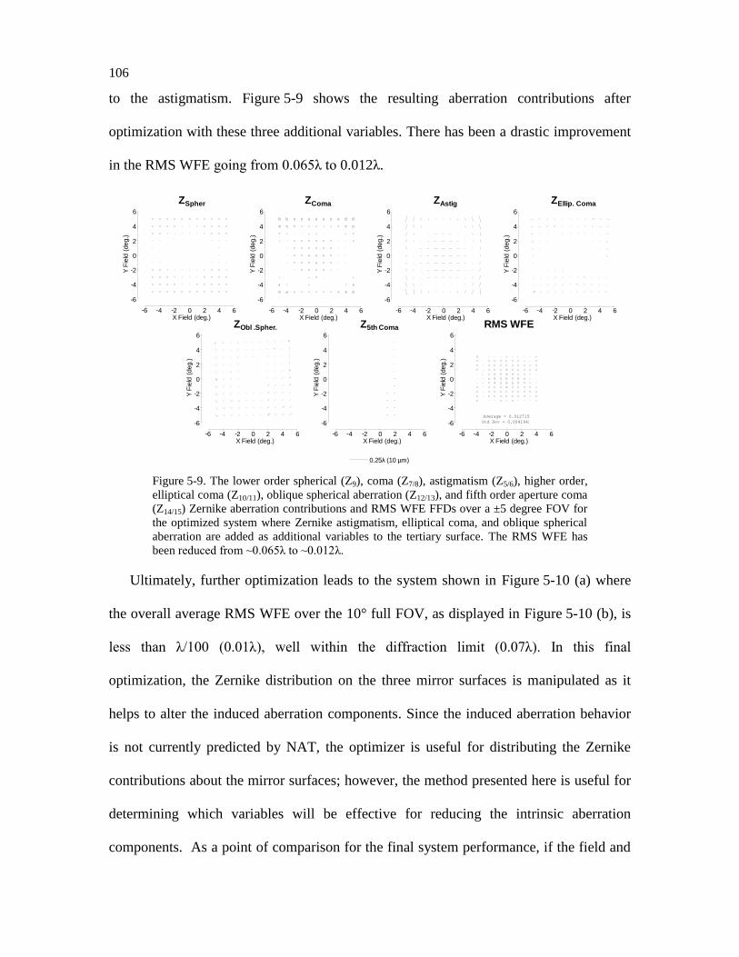
106
to the astigmatism. Figure 5-9 shows the resulting aberration contributions after
optimization with these three additional variables. There has been a drastic improvement
in the RMS WFE going from 0.065λ to 0.012λ.
14:37:40
Zernike Polynomial
KHF 23-Sep-13
FRINGE ZERNIKE PAIR Z5 AND Z6
vs
FIELD ANGLE IN OBJECT SPACE
Minimum = 0.0030928
Maximum = 0.10011
Average = 0.032326
Std Dev = 0.021346
0.25waves (10000.0 nm)
-6 -4 -2 0 2 4 6
X Field Angle in Object Space - degrees
-6
-4
-2
0
2
4
6
Y Field Angle in Object Space - degrees
14:37:41
Zernike Polynomial
KHF 23-Sep-13
FRINGE ZERNIKE PAIR Z7 AND Z8
vs
FIELD ANGLE IN OBJECT SPACE
Minimum = 0.0012659
Maximum = 0.046904
Average = 0.01482
Std Dev = 0.0091452
0.25waves (10000.0 nm)
-6 -4 -2 0 2 4 6
X Field Angle in Object Space - degrees
-6
-4
-2
0
2
4
6
Y Field Angle in Object Space - degrees
14:37:41
Zernike Polynomial
KHF 23-Sep-13
FRINGE ZERNIKE COEFFICIENT Z9
vs
FIELD ANGLE IN OBJECT SPACE
Minimum = -0.015258
Maximum = 0.012736
Average = 0.00036325
Std Dev = 0.0086811
0.25waves (10000.0 nm)
-6 -4 -2 0 2 4 6
X Field Angle in Object Space - degrees
-6
-4
-2
0
2
4
6
Y Field Angle in Object Space - degrees
14:37:41
Zernike Polynomial
KHF 23-Sep-13
FRINGE ZERNIKE PAIR Z10 AND Z11
vs
FIELD ANGLE IN OBJECT SPACE
Minimum = 0.00011767
Maximum = 0.035384
Average = 0.011416
Std Dev = 0.0077174
0.25waves (10000.0 nm)
-6 -4 -2 0 2 4 6
X Field Angle in Object Space - degrees
-6
-4
-2
0
2
4
6
Y Field Angle in Object Space - degrees
14:37:41
Zernike Polynomial
KHF 23-Sep-13
FRINGE ZERNIKE PAIR Z12 AND Z13
vs
FIELD ANGLE IN OBJECT SPACE
Minimum = 0.0012925
Maximum = 0.028797
Average = 0.016026
Std Dev = 0.0062967
0.25waves (10000.0 nm)
-6 -4 -2 0 2 4 6
X Field Angle in Object Space - degrees
-6
-4
-2
0
2
4
6
Y Field Angle in Object Space - degrees
14:37:41
Zernike Polynomial
KHF 23-Sep-13
FRINGE ZERNIKE PAIR Z14 AND Z15
vs
FIELD ANGLE IN OBJECT SPACE
Minimum = 0.0001119
Maximum = 0.0060283
Average = 0.0032851
Std Dev = 0.0013844
0.25waves (10000.0 nm)
-6 -4 -2 0 2 4 6
X Field Angle in Object Space - degrees
-6
-4
-2
0
2
4
6
Y Field Angle in Object Space - degrees
14:37:42
Zernike Polynomial
KHF 23-Sep-13
RMS WAVEFRONT ERROR
vs
FIELD ANGLE IN OBJECT SPACE
Minimum = 0.0066824
Maximum = 0.021031
Average = 0.012715
Std Dev = 0.0041642
0.25waves (10000.0 nm)
-6 -4 -2 0 2 4 6
X Field Angle in Object Space - degrees
-6
-4
-2
0
2
4
6
Y Field Angle in Object Space - degrees
ZEllip. Coma
ZObl .Spher. RMS WFE
ZAstigZComaZSpher
Z5th Coma
6 4 2 0 642- - -X Field (deg.)
6-
4-
2-
0
2
4
6
Y F
ield
(deg.)
6 4 2 0 642- - -X Field (deg.)
6-
4-
2-
0
2
4
6
Y F
ield
(deg.)
6 4 2 0 642- - -X Field (deg.)
6-
4-
2-
0
2
4
6
Y F
ield
(deg.)
6 4 2 0 642- - -X Field (deg.)
6-
4-
2-
0
2
4
6
Y F
ield
(deg.)
6 4 2 0 642- - -X Field (deg.)
6-
4-
2-
0
2
4
6
Y F
ield
(deg.)
6 4 2 0 642- - -X Field (deg.)
6-
4-
2-
0
2
4
6
Y F
ield
(deg.)
6 4 2 0 642- - -X Field (deg.)
6-
4-
2-
0
2
4
6
Y F
ield
(deg.)
14:37:41
Zernike Polynomial
KHF 23-Sep-13
FRINGE ZERNIKE COEFFICIENT Z9
vs
FIELD ANGLE IN OBJECT SPACE
Minimum = -0.015258
Maximum = 0.012736
Average = 0.00036325
Std Dev = 0.0086811
0.25waves (10000.0 nm)
-6 -4 -2 0 2 4 6
X Field Angle in Object Space - degrees
-6
-4
-2
0
2
4
6
Y Field Angle in Object Space - degrees
0.25λ (10 µm)
14:37:42
Zernike Polynomial
KHF 23-Sep-13
RMS WAVEFRONT ERROR
vs
FIELD ANGLE IN OBJECT SPACE
Minimum = 0.0066824
Maximum = 0.021031
Average = 0.012715
Std Dev = 0.0041642
0.25waves (10000.0 nm)
-6 -4 -2 0 2 4 6
X Field Angle in Object Space - degrees
-6
-4
-2
0
2
4
6
Y Field Angle in Object Space - degrees
Figure 5-9. The lower order spherical (Z9), coma (Z7/8), astigmatism (Z5/6), higher order,
elliptical coma (Z10/11), oblique spherical aberration (Z12/13), and fifth order aperture coma
(Z14/15) Zernike aberration contributions and RMS WFE FFDs over a ±5 degree FOV for
the optimized system where Zernike astigmatism, elliptical coma, and oblique spherical
aberration are added as additional variables to the tertiary surface. The RMS WFE has
been reduced from ~0.065λ to ~0.012λ.
Ultimately, further optimization leads to the system shown in Figure 5-10 (a) where
the overall average RMS WFE over the 10° full FOV, as displayed in Figure 5-10 (b), is
less than λ/100 (0.01λ), well within the diffraction limit (0.07λ). In this final
optimization, the Zernike distribution on the three mirror surfaces is manipulated as it
helps to alter the induced aberration components. Since the induced aberration behavior
is not currently predicted by NAT, the optimizer is useful for distributing the Zernike
contributions about the mirror surfaces; however, the method presented here is useful for
determining which variables will be effective for reducing the intrinsic aberration
components. As a point of comparison for the final system performance, if the field and
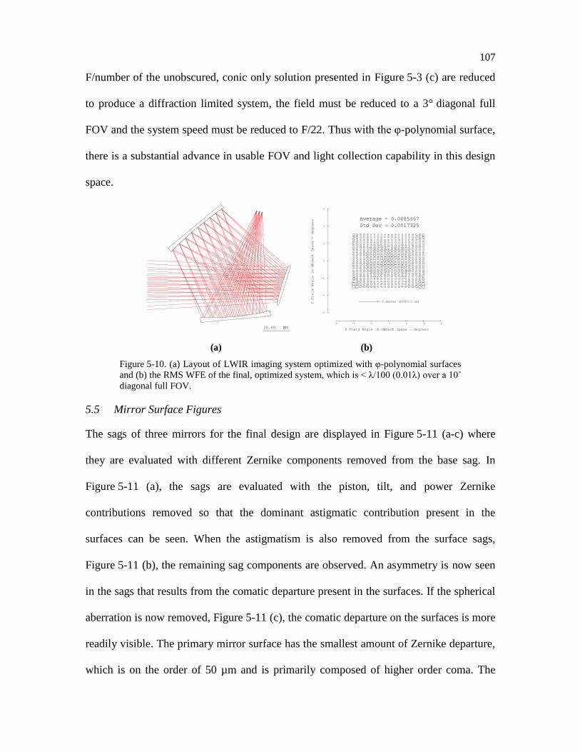
107
F/number of the unobscured, conic only solution presented in Figure 5-3 (c) are reduced
to produce a diffraction limited system, the field must be reduced to a 3° diagonal full
FOV and the system speed must be reduced to F/22. Thus with the φ-polynomial surface,
there is a substantial advance in usable FOV and light collection capability in this design
space.
(a) (b)
14:25:51
Zernike Polynomial FULL SCALE KHF 17-Sep-11
25.00 MM
14:25:51
Zernike Polynomial FULL SCALE KHF 17-Sep-11
25.00 MM
16:54:26
Zernike Polynomial
KHF 26-Sep-11
RMS WAVEFRONT ERROR
vs
FIELD ANGLE IN OBJECT SPACE
Minimum = 0.0049516
Maximum = 0.015382
Average = 0.0085467
Std Dev = 0.0017325
0.1waves (10000.0 nm)
-6 -4 -2 0 2 4 6
X Field Angle in Object Space - degrees
-6
-4
-2
0
2
4
6
Y Field Angle in Object Space - degrees
Figure 5-10. (a) Layout of LWIR imaging system optimized with φ-polynomial surfaces
and (b) the RMS WFE of the final, optimized system, which is < λ/100 (0.01λ) over a 10˚
diagonal full FOV.
5.5 Mirror Surface Figures
The sags of three mirrors for the final design are displayed in Figure 5-11 (a-c) where
they are evaluated with different Zernike components removed from the base sag. In
Figure 5-11 (a), the sags are evaluated with the piston, tilt, and power Zernike
contributions removed so that the dominant astigmatic contribution present in the
surfaces can be seen. When the astigmatism is also removed from the surface sags,
Figure 5-11 (b), the remaining sag components are observed. An asymmetry is now seen
in the sags that results from the comatic departure present in the surfaces. If the spherical
aberration is now removed, Figure 5-11 (c), the comatic departure on the surfaces is more
readily visible. The primary mirror surface has the smallest amount of Zernike departure,
which is on the order of 50 µm and is primarily composed of higher order coma. The
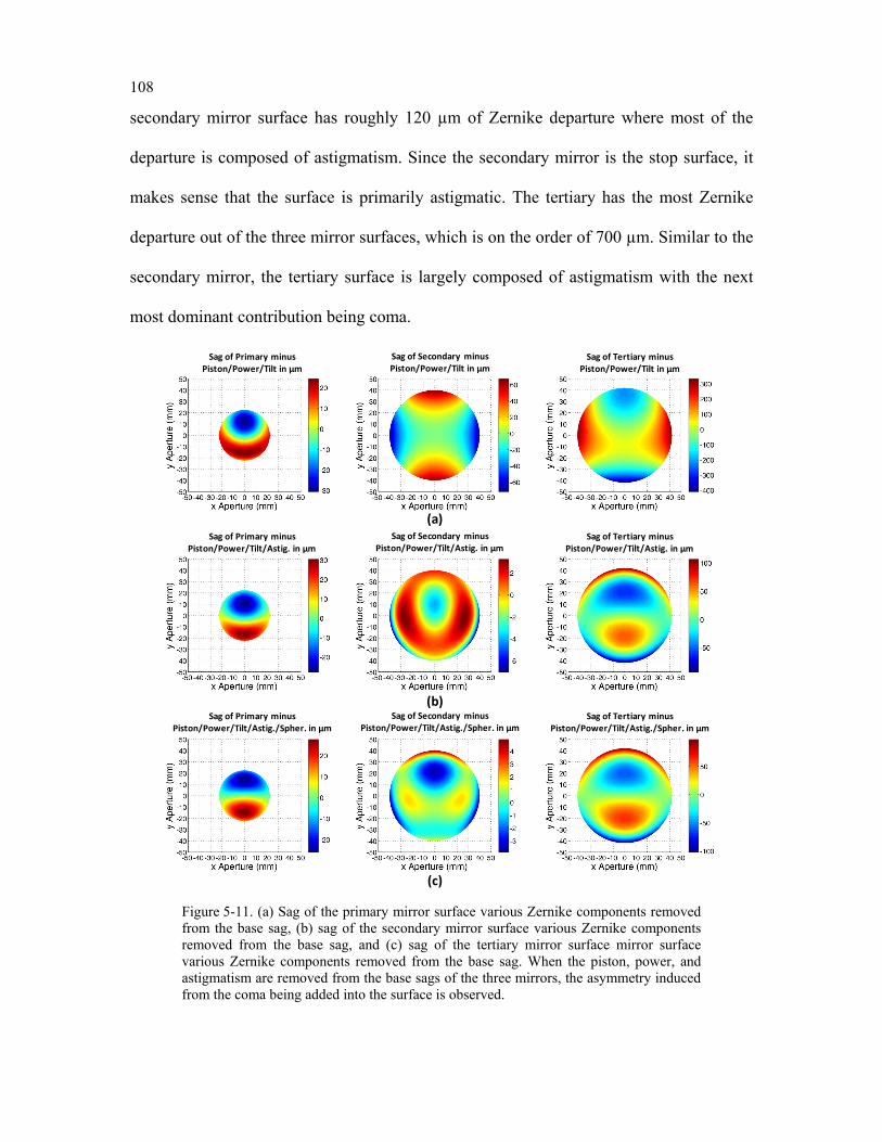
108
secondary mirror surface has roughly 120 µm of Zernike departure where most of the
departure is composed of astigmatism. Since the secondary mirror is the stop surface, it
makes sense that the surface is primarily astigmatic. The tertiary has the most Zernike
departure out of the three mirror surfaces, which is on the order of 700 µm. Similar to the
secondary mirror, the tertiary surface is largely composed of astigmatism with the next
most dominant contribution being coma.
(a)
(b)
(c)
Sag of Secondary minus Piston/Power/Tilt in µm
Sag of Secondary minus Piston/Power/Tilt/Astig. in µm
Sag of Secondary minus Piston/Power/Tilt/Astig./Spher. in µm
Sag of Tertiary minus Piston/Power/Tilt in µm
Sag of Tertiary minus Piston/Power/Tilt/Astig. in µm
Sag of Tertiary minus Piston/Power/Tilt/Astig./Spher. in µm
Sag of Primary minus Piston/Power/Tilt in µm
Sag of Primary minus Piston/Power/Tilt/Astig. in µm
Sag of Primary minus Piston/Power/Tilt/Astig./Spher. in µm
Figure 5-11. (a) Sag of the primary mirror surface various Zernike components removed from the base sag, (b) sag of the secondary mirror surface various Zernike components removed from the base sag, and (c) sag of the tertiary mirror surface mirror surface various Zernike components removed from the base sag. When the piston, power, and astigmatism are removed from the base sags of the three mirrors, the asymmetry induced from the coma being added into the surface is observed.
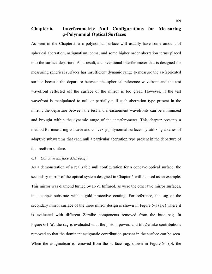
109
Chapter 6. Interferometric Null Configurations for Measuring φ-Polynomial Optical Surfaces
As seen in the Chapter 5, a φ-polynomial surface will usually have some amount of
spherical aberration, astigmatism, coma, and some higher order aberration terms placed
into the surface departure. As a result, a conventional interferometer that is designed for
measuring spherical surfaces has insufficient dynamic range to measure the as-fabricated
surface because the departure between the spherical reference wavefront and the test
wavefront reflected off the surface of the mirror is too great. However, if the test
wavefront is manipulated to null or partially null each aberration type present in the
mirror, the departure between the test and measurement wavefronts can be minimized
and brought within the dynamic range of the interferometer. This chapter presents a
method for measuring concave and convex φ-polynomial surfaces by utilizing a series of
adaptive subsystems that each null a particular aberration type present in the departure of
the freeform surface.
6.1 Concave Surface Metrology
As a demonstration of a realizable null configuration for a concave optical surface, the
secondary mirror of the optical system designed in Chapter 5 will be used as an example.
This mirror was diamond turned by II-VI Infrared, as were the other two mirror surfaces,
in a copper substrate with a gold protective coating. For reference, the sag of the
secondary mirror surface of the three mirror design is shown in Figure 6-1 (a-c) where it
is evaluated with different Zernike components removed from the base sag. In
Figure 6-1 (a), the sag is evaluated with the piston, power, and tilt Zernike contributions
removed so that the dominant astigmatic contribution present in the surface can be seen.
When the astigmatism is removed from the surface sag, shown in Figure 6-1 (b), the
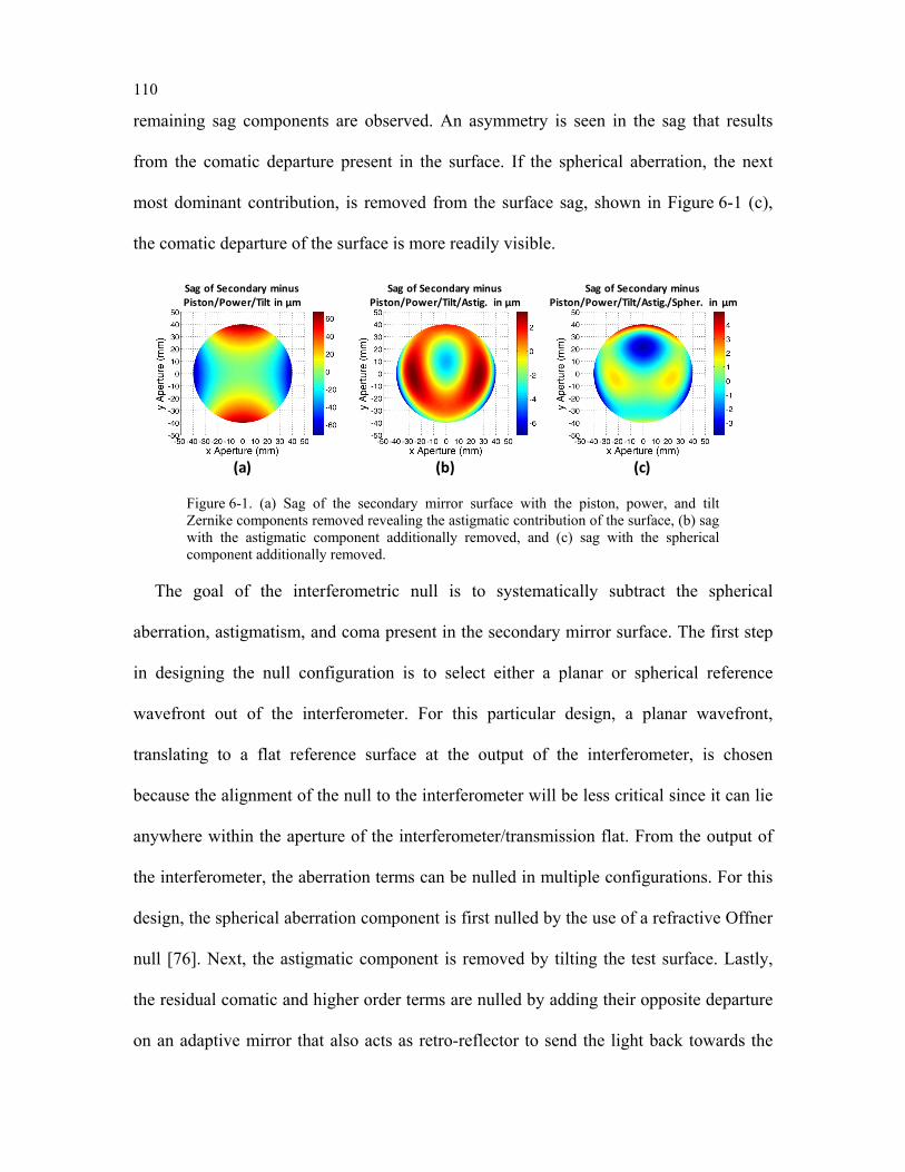
110
remaining sag components are observed. An asymmetry is seen in the sag that results
from the comatic departure present in the surface. If the spherical aberration, the next
most dominant contribution, is removed from the surface sag, shown in Figure 6-1 (c),
the comatic departure of the surface is more readily visible.
(a) (b) (c)
Sag of Secondary minus Piston/Power/Tilt in µm
Sag of Secondary minus Piston/Power/Tilt/Astig. in µm
Sag of Secondary minus Piston/Power/Tilt/Astig./Spher. in µm
Figure 6-1. (a) Sag of the secondary mirror surface with the piston, power, and tilt Zernike components removed revealing the astigmatic contribution of the surface, (b) sag with the astigmatic component additionally removed, and (c) sag with the spherical component additionally removed.
The goal of the interferometric null is to systematically subtract the spherical
aberration, astigmatism, and coma present in the secondary mirror surface. The first step
in designing the null configuration is to select either a planar or spherical reference
wavefront out of the interferometer. For this particular design, a planar wavefront,
translating to a flat reference surface at the output of the interferometer, is chosen
because the alignment of the null to the interferometer will be less critical since it can lie
anywhere within the aperture of the interferometer/transmission flat. From the output of
the interferometer, the aberration terms can be nulled in multiple configurations. For this
design, the spherical aberration component is first nulled by the use of a refractive Offner
null [76]. Next, the astigmatic component is removed by tilting the test surface. Lastly,
the residual comatic and higher order terms are nulled by adding their opposite departure
on an adaptive mirror that also acts as retro-reflector to send the light back towards the
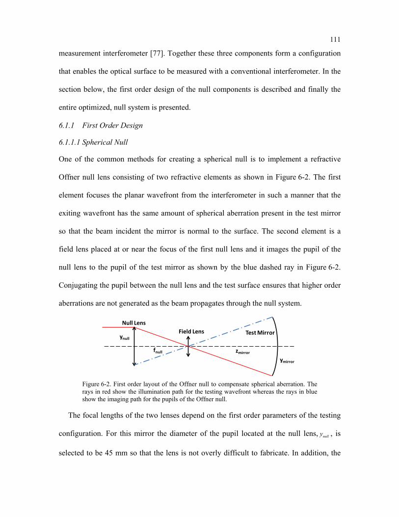
111
measurement interferometer [77]. Together these three components form a configuration
that enables the optical surface to be measured with a conventional interferometer. In the
section below, the first order design of the null components is described and finally the
entire optimized, null system is presented.
6.1.1 First Order Design
6.1.1.1 Spherical Null
One of the common methods for creating a spherical null is to implement a refractive
Offner null lens consisting of two refractive elements as shown in Figure 6-2. The first
element focuses the planar wavefront from the interferometer in such a manner that the
exiting wavefront has the same amount of spherical aberration present in the test mirror
so that the beam incident the mirror is normal to the surface. The second element is a
field lens placed at or near the focus of the first null lens and it images the pupil of the
null lens to the pupil of the test mirror as shown by the blue dashed ray in Figure 6-2.
Conjugating the pupil between the null lens and the test surface ensures that higher order
aberrations are not generated as the beam propagates through the null system.
Test MirrorField LensNull Lens
fnull zmirror
ynull
ymirror
Figure 6-2. First order layout of the Offner null to compensate spherical aberration. The rays in red show the illumination path for the testing wavefront whereas the rays in blue show the imaging path for the pupils of the Offner null.
The focal lengths of the two lenses depend on the first order parameters of the testing
configuration. For this mirror the diameter of the pupil located at the null lens, nully , is
selected to be 45 mm so that the lens is not overly difficult to fabricate. In addition, the
112
region of interest on the mirror, mirrory , is 70 mm and to keep the overall length of the null
system small, the distance between the focus of the null lens and the test mirror, mirrorz , is
chosen to be at or near the radius of curvature of the mirror under test, which for this
system has been chosen to be 367.5 mm. Based on these parameters, the focal length of
the null lens, nullf , is computed using the magnification as,
,mirrornull null
mirror
zf y
y
=
(6.1)
and yields for the parameters described above, a null lens focal length of 234.6 mm. From
the null lens focal length, the focal length of the field lens is computed from the thin lens
equation as,
1
1 1 ,fieldmirror null
fz f
−
= −
(6.2)
and yields a field lens focal length of 143.2 mm.
Now that the first order parameters of the Offner null have been computed, the next
step is to select the curvatures for the null lens that will yield the correct amount of
spherical aberration to create a null for the mirror under test. Since the null lens and
mirror are conjugate to one another, the Fringe Zernike spherical contribution on the
mirror surface, 9Mirrorz , is related to the required null lens spherical wave aberration, 040
NullW ,
by taking the opposite transmitted wavefront aberration of the mirror calculated as,
040 96 ( 1 1).Null MirrorW z= − − − (6.3)
where the refractive index of the mirror is assumed to be -1. For the 2.5 µm of Fringe
Zernike spherical present in the test mirror, 30 µm of spherical wave aberration must be
created by the null lens. From the required wave aberration of the null lens, the equation
113
for spherical aberration of a thin lens at the stop surface [55] is rearranged to compute the
required shape factor, Nullβ , for the null lens and is given by,
( ) ( )1/2
22 232 1
040 42 1
2 1 132,
2 1 2 2
Null NullNull Null
Null Null NullNull
n n nfR R n nWn n n nR R y
β − − + = = + − + + − + +−
(6.4)
where 1NullR and 2
NullR are the front and back radius of curvature of the null lens and n is the
refractive index of the lens. For ease of fabrication, NBK7 glass is chosen, which has a
refractive index of 1.515 at interferometer testing wavelength of 632.8nm. Substituting
all known parameters in Eq. (6.4) leads to a shape factor of roughly 2.81, which indicates
a strong meniscus for the null lens. Finally using the relation of the curvature of the null
lens to the focal length and shape factor, the front and back radius of curvature is
computed as,
( )( )1/2
2 1,
1Null f n
Rβ
−=
± (6.5)
where after substitution, the two radii come to 62.29 mm and 128.57 mm, respectively.
With all the first order parameters of the Offner null calculated, the next step is to
calculate the required tilt angle of the test mirror to null astigmatism.
6.1.1.2 Astigmatic Null
When a spherical mirror is operated off-axis at or near the center of curvature, the
dominant aberration is third order astigmatism. The astigmatism is minimized by adding
a toroidal shape to the mirror. The principal radii of curvature, xR and yR , that determine
the ideal toroidal mirror to minimize astigmatism are found by the Coddington equations
[78] that are expressed for a mirror as,
( )
1 1 2' costT T R i+ = (6.6)
and
114
( )2cos1 1 ,' x
iS S R
+ = (6.7)
where T and S are the distances from the tangential (T) and sagittal (S) astigmatic focal
surfaces of the object to the mirror, T’ and S’ are the distances from the mirror to the
astigmatic focal surfaces of the image, and i is the angle of the mirror with respect to the
optical axis in the YZ plane. If the object and image are to be anastigmatic, T must be
equivalent to S as well as T’ must also be equal to S’. In this special case, Eq. (6.6)
and (6.7) reduce to,
( )2cos ,x
y
Ri
R= (6.8)
where x yR R< for there to be a valid mirror angle, i . For the case where y xR R< , the
mirror angle, i , must be re-defined in the XZ plane, so that Eq. (6.8) becomes,
( )2cos .y
x
Ri
R= (6.9)
For the mirror of interest, a toroidal shape has been intentionally polished into the
surface by prescribing some combination of primary and secondary Zernike astigmatism.
Following Eq. (6.8), in order to null the toroidal shape, the mirror must be tilted at an
angle where the angle depends on the principal radii of curvature. The principal radii of
curvature are derived from the Zernike terms present in the mirror surface by following a
method proposed by Schwiegerling et al. [79]. In this method, the sag of the optical
surface with the Fringe Zernike overlay is approximated as parabolic, so that the sag
along the x-direction is written as,
2 2 2 22 2
4 8 5 122 6 3 ,2 2x
x B N N N N
sag z z z zR R R R R Rρ ρ ρ ρ ρ ρ
= = + − + −
(6.10)
and the sag in the y-direction is written as,
115
2 2 2 22 2
4 8 5 122 6 3 ,2 2y
y B N N N N
sag z z z zR R R R R Rρ ρ ρ ρ ρ ρ
= = + − − +
(6.11)
where BR is the base radius of curvature of the mirror, ρ is the radial coordinate, NR is the
normalizing radius of Fringe Zernike overlay, and 4,8,5,12z are the Fringe Zernike
coefficients for power, spherical aberration, astigmatism, and oblique spherical
aberration. By simplifying and manipulating Eq. (6.10) and (6.11), xR and yR are
computed as,
2
/ 2
4 8 5 12
.2 2 6
2
Nx y
N
B
RR
R z z z zR
=
+ − ±
(6.12)
After substituting the prescription parameters of the mirror in Eq. (6.12), xR and yR are
calculated to be -394.2 mm and -371.4 mm leading to a tilt angle from Eq. (6.8) of
13.91°. More specifically, if the mirror under test is tilted at 13.91° then the astigmatic
contribution from the mirror will be nulled. However, an obstacle to overcome with a
tilted geometry is that the reflected wavefront from the mirror will no longer be reflected
back on itself and requires the use of an additional element to return the test wavefront
back to the interferometer. In this case, a deformable mirror (DM) that is nominally flat
but can be deformed into a wide variety of shapes is employed. It provides
retro-reflection without inversion and also nulls the residual coma and any higher order
aberrations present in the test wavefront.
6.1.1.3 Comatic and Higher Order Null
In order to use the quasi-flat DM, the wavefront reflected off the test mirror must be
collimated with the use of a collimating lens. In addition, the DM with a clear aperture of
15 mm must also be conjugate to the test mirror. This configuration is diagramed in
Figure 6-3 where the illumination path from the interferometer is shown in red and the
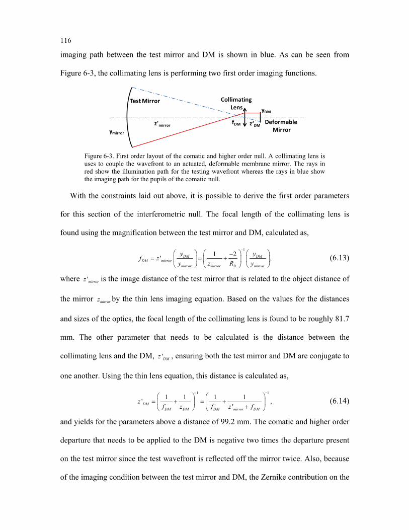
116
imaging path between the test mirror and DM is shown in blue. As can be seen from
Figure 6-3, the collimating lens is performing two first order imaging functions.
Test Mirror Collimating Lens
fDMz'mirror
yDM
ymirror
Deformable Mirror
z‘DM
Figure 6-3. First order layout of the comatic and higher order null. A collimating lens is uses to couple the wavefront to an actuated, deformable membrane mirror. The rays in red show the illumination path for the testing wavefront whereas the rays in blue show the imaging path for the pupils of the comatic null.
With the constraints laid out above, it is possible to derive the first order parameters
for this section of the interferometric null. The focal length of the collimating lens is
found using the magnification between the test mirror and DM, calculated as,
1
1 2' ,DM DMDM mirror
mirror mirror B mirror
y yf zy z R y
− −
= = +
(6.13)
where 'mirrorz is the image distance of the test mirror that is related to the object distance of
the mirror mirrorz by the thin lens imaging equation. Based on the values for the distances
and sizes of the optics, the focal length of the collimating lens is found to be roughly 81.7
mm. The other parameter that needs to be calculated is the distance between the
collimating lens and the DM, 'DMz , ensuring both the test mirror and DM are conjugate to
one another. Using the thin lens equation, this distance is calculated as,
11
1 1 1 1' ,'DM
DM DM DM mirror DM
zf z f z f
−−
= + = + +
(6.14)
and yields for the parameters above a distance of 99.2 mm. The comatic and higher order
departure that needs to be applied to the DM is negative two times the departure present
on the test mirror since the test wavefront is reflected off the mirror twice. Also, because
of the imaging condition between the test mirror and DM, the Zernike contribution on the
117
DM must be rotated by 180°. With all paraxial parameters for the inteferometric null now
established, the null configuration can now be optimized using commercially available
lens design software to provide a final thick lens solution.
6.1.2 Optimization of the Interferometric Null System
The paraxial solution described in the section above creates a starting point for further
optimization. The end goal for optimization is to produce a double pass, thick lens
solution that provides a null or quasi-null wavefront exiting the interferometric system.
Using CODE V, user defined constraints are written for nulling the Fringe Zernike
spherical aberration, astigmatism, coma, and any higher order aberration terms while
maintaining conjugates between nulling components. As for the parameters allowed to
vary during optimization, the radii of the null lens are roughly set by the first and third
order constraints but are allowed to vary to account for variations from the lens thickness;
however, the focal length is kept fixed to its first order value. For the field lens, the lens
has been chosen to be NBK7. Since the size of the beam footprint at the field lens is
small, it introduces little spherical aberration, so for ease of fabrication, positioning, and
alignment, its shape is chosen to be bi-convex. The focal length is allowed to vary from
its paraxial value because the field lens parameters can be used to minimize higher order
spherical aberration. The collimating lens near the DM is chosen to be a high index
material, SF6, so it introduces less spherical aberration. For ease of fabrication and to
introduce as little spherical aberration as possible, the shape is chosen to be plano-convex
as it is near the shape factor for minimum spherical aberration. The focal length is kept
roughly the same as its first order value to ensure that the size of the beam on the DM
does not exceed 15 mm. The mirror tilt about the y-axis is allowed to vary from its
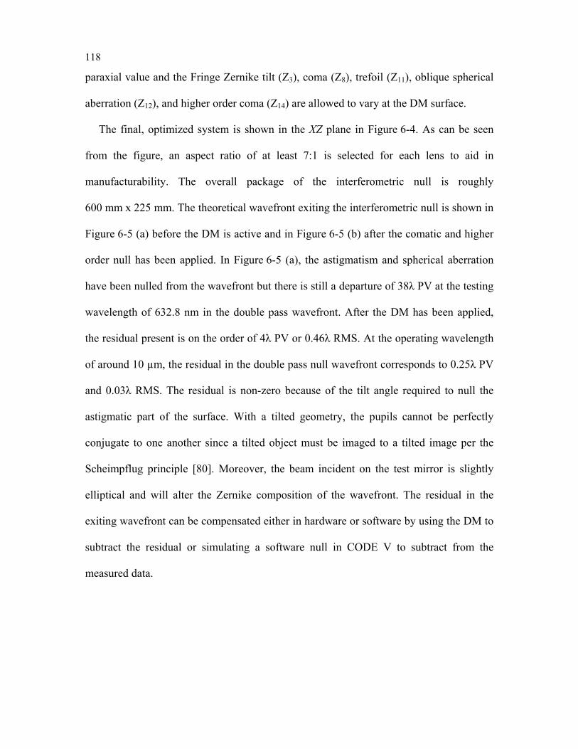
118
paraxial value and the Fringe Zernike tilt (Z3), coma (Z8), trefoil (Z11), oblique spherical
aberration (Z12), and higher order coma (Z14) are allowed to vary at the DM surface.
The final, optimized system is shown in the XZ plane in Figure 6-4. As can be seen
from the figure, an aspect ratio of at least 7:1 is selected for each lens to aid in
manufacturability. The overall package of the interferometric null is roughly
600 mm x 225 mm. The theoretical wavefront exiting the interferometric null is shown in
Figure 6-5 (a) before the DM is active and in Figure 6-5 (b) after the comatic and higher
order null has been applied. In Figure 6-5 (a), the astigmatism and spherical aberration
have been nulled from the wavefront but there is still a departure of 38λ PV at the testing
wavelength of 632.8 nm in the double pass wavefront. After the DM has been applied,
the residual present is on the order of 4λ PV or 0.46λ RMS. At the operating wavelength
of around 10 µm, the residual in the double pass null wavefront corresponds to 0.25λ PV
and 0.03λ RMS. The residual is non-zero because of the tilt angle required to null the
astigmatic part of the surface. With a tilted geometry, the pupils cannot be perfectly
conjugate to one another since a tilted object must be imaged to a tilted image per the
Scheimpflug principle [80]. Moreover, the beam incident on the test mirror is slightly
elliptical and will alter the Zernike composition of the wavefront. The residual in the
exiting wavefront can be compensated either in hardware or software by using the DM to
subtract the residual or simulating a software null in CODE V to subtract from the
measured data.
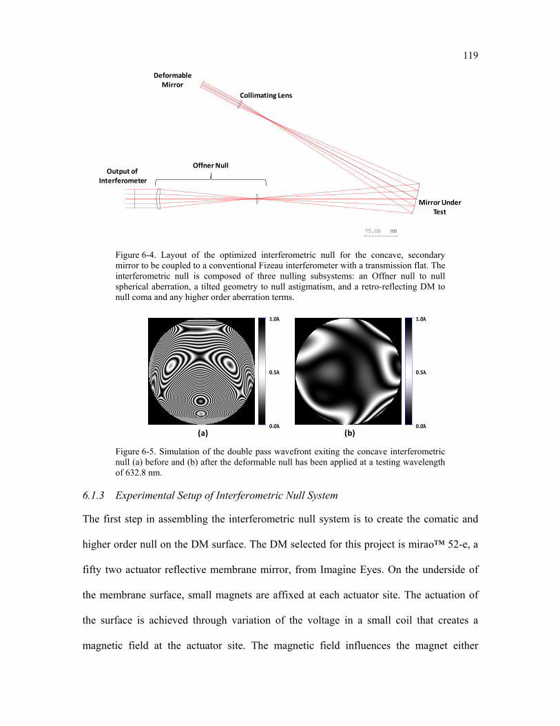
119
75.00 MM
Output of Interferometer
Offner Null
DeformableMirror
Mirror UnderTest
Collimating Lens
Figure 6-4. Layout of the optimized interferometric null for the concave, secondary mirror to be coupled to a conventional Fizeau interferometer with a transmission flat. The interferometric null is composed of three nulling subsystems: an Offner null to null spherical aberration, a tilted geometry to null astigmatism, and a retro-reflecting DM to null coma and any higher order aberration terms.
0.0λ
0.5λ
1.0λ
0.0λ
0.5λ
1.0λ
(a) (b)0
1
0
0
1
0
Figure 6-5. Simulation of the double pass wavefront exiting the concave interferometric null (a) before and (b) after the deformable null has been applied at a testing wavelength of 632.8 nm.
6.1.3 Experimental Setup of Interferometric Null System
The first step in assembling the interferometric null system is to create the comatic and
higher order null on the DM surface. The DM selected for this project is mirao™ 52-e, a
fifty two actuator reflective membrane mirror, from Imagine Eyes. On the underside of
the membrane surface, small magnets are affixed at each actuator site. The actuation of
the surface is achieved through variation of the voltage in a small coil that creates a
magnetic field at the actuator site. The magnetic field influences the magnet either
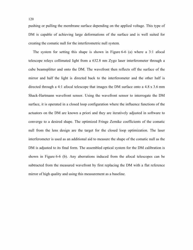
120
pushing or pulling the membrane surface depending on the applied voltage. This type of
DM is capable of achieving large deformations of the surface and is well suited for
creating the comatic null for the interferometric null system.
The system for setting this shape is shown in Figure 6-6 (a) where a 3:1 afocal
telescope relays collimated light from a 632.8 nm Zygo laser interferometer through a
cube beamsplitter and onto the DM. The wavefront then reflects off the surface of the
mirror and half the light is directed back to the interferometer and the other half is
directed through a 4:1 afocal telescope that images the DM surface onto a 4.8 x 3.6 mm
Shack-Hartmann wavefront sensor. Using the wavefront sensor to interrogate the DM
surface, it is operated in a closed loop configuration where the influence functions of the
actuators on the DM are known a priori and they are iteratively adjusted in software to
converge to a desired shape. The optimized Fringe Zernike coefficients of the comatic
null from the lens design are the target for the closed loop optimization. The laser
interferometer is used as an additional aid to measure the shape of the comatic null as the
DM is adjusted to its final form. The assembled optical system for the DM calibration is
shown in Figure 6-6 (b). Any aberrations induced from the afocal telescopes can be
subtracted from the measured wavefront by first replacing the DM with a flat reference
mirror of high quality and using this measurement as a baseline.
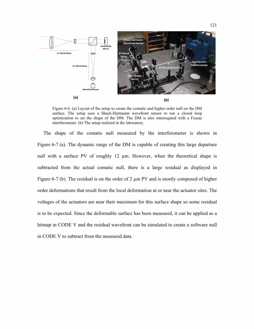
121
Deformable Mirror
Wavefront Sensor
3:1 Afocal Relay
4:1 Afocal Relay
DeformableMirror
4F Afocal Relay (3:1)
4F AfocalRelay (4:1)
Shack-Hartmann Wavefront Sensor
Zygo DynaFizInterferometer
(a)(b)
Figure 6-6. (a) Layout of the setup to create the comatic and higher order null on the DM surface. The setup uses a Shack-Hartmann wavefront sensor to run a closed loop optimization to set the shape of the DM. The DM is also interrogated with a Fizeau interferometer. (b) The setup realized in the laboratory.
The shape of the comatic null measured by the interferometer is shown in
Figure 6-7 (a). The dynamic range of the DM is capable of creating this large departure
null with a surface PV of roughly 12 µm. However, when the theoretical shape is
subtracted from the actual comatic null, there is a large residual as displayed in
Figure 6-7 (b). The residual is on the order of 2 µm PV and is mostly composed of higher
order deformations that result from the local deformation at or near the actuator sites. The
voltages of the actuators are near their maximum for this surface shape so some residual
is to be expected. Since the deformable surface has been measured, it can be applied as a
hitmap in CODE V and the residual wavefront can be simulated to create a software null
in CODE V to subtract from the measured data.
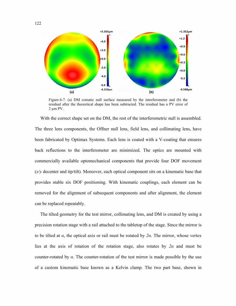
122
(a) (b)
+5.565µm
-6.310µm
-6.0
+0.0
-4.0
-2.0
+2.0
+4.0
+1.352µm
-0.588µm
+1.2
+0.3
-0.3
+0.0
+0.6
+0.9
Figure 6-7. (a) DM comatic null surface measured by the interferometer and (b) the residual after the theoretical shape has been subtracted. The residual has a PV error of 2 µm PV.
With the correct shape set on the DM, the rest of the interferometric null is assembled.
The three lens components, the Offner null lens, field lens, and collimating lens, have
been fabricated by Optimax Systems. Each lens is coated with a V-coating that ensures
back reflections to the interferometer are minimized. The optics are mounted with
commercially available optomechanical components that provide four DOF movement
(x/y decenter and tip/tilt). Moreover, each optical component sits on a kinematic base that
provides stable six DOF positioning. With kinematic couplings, each element can be
removed for the alignment of subsequent components and after alignment, the element
can be replaced repeatably.
The tilted geometry for the test mirror, collimating lens, and DM is created by using a
precision rotation stage with a rail attached to the tabletop of the stage. Since the mirror is
to be tilted at α, the optical axis or rail must be rotated by 2α. The mirror, whose vertex
lies at the axis of rotation of the rotation stage, also rotates by 2α and must be
counter-rotated by α. The counter-rotation of the test mirror is made possible by the use
of a custom kinematic base known as a Kelvin clamp. The two part base, shown in
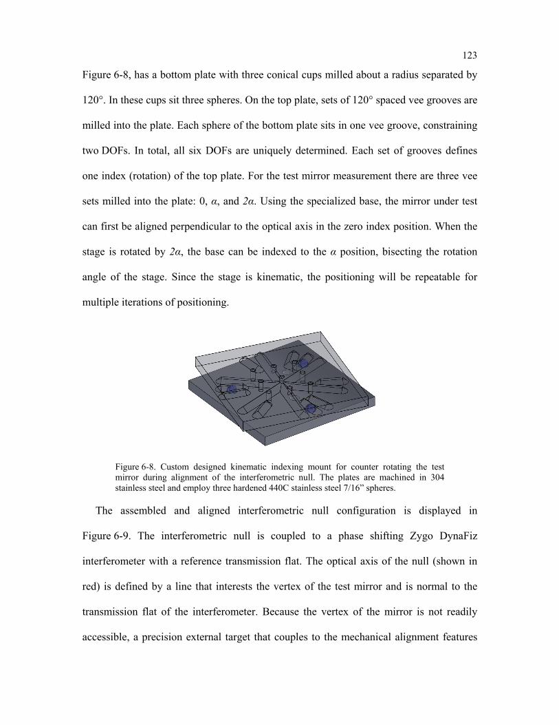
123
Figure 6-8, has a bottom plate with three conical cups milled about a radius separated by
120°. In these cups sit three spheres. On the top plate, sets of 120° spaced vee grooves are
milled into the plate. Each sphere of the bottom plate sits in one vee groove, constraining
two DOFs. In total, all six DOFs are uniquely determined. Each set of grooves defines
one index (rotation) of the top plate. For the test mirror measurement there are three vee
sets milled into the plate: 0, α, and 2α. Using the specialized base, the mirror under test
can first be aligned perpendicular to the optical axis in the zero index position. When the
stage is rotated by 2α, the base can be indexed to the α position, bisecting the rotation
angle of the stage. Since the stage is kinematic, the positioning will be repeatable for
multiple iterations of positioning.
Figure 6-8. Custom designed kinematic indexing mount for counter rotating the test mirror during alignment of the interferometric null. The plates are machined in 304 stainless steel and employ three hardened 440C stainless steel 7/16” spheres.
The assembled and aligned interferometric null configuration is displayed in
Figure 6-9. The interferometric null is coupled to a phase shifting Zygo DynaFiz
interferometer with a reference transmission flat. The optical axis of the null (shown in
red) is defined by a line that interests the vertex of the test mirror and is normal to the
transmission flat of the interferometer. Because the vertex of the mirror is not readily
accessible, a precision external target that couples to the mechanical alignment features
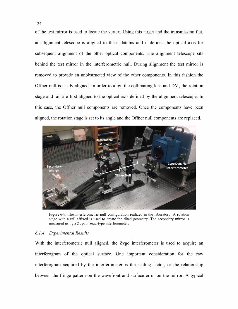
124
of the test mirror is used to locate the vertex. Using this target and the transmission flat,
an alignment telescope is aligned to these datums and it defines the optical axis for
subsequent alignment of the other optical components. The alignment telescope sits
behind the test mirror in the interferometric null. During alignment the test mirror is
removed to provide an unobstructed view of the other components. In this fashion the
Offner null is easily aligned. In order to align the collimating lens and DM, the rotation
stage and rail are first aligned to the optical axis defined by the alignment telescope. In
this case, the Offner null components are removed. Once the components have been
aligned, the rotation stage is set to its angle and the Offner null components are replaced.
Offner Null
DeformableMirror
SecondaryMirror
Zygo DynaFizInterferometer
Figure 6-9. The interferometric null configuration realized in the laboratory. A rotation stage with a rail affixed is used to create the tilted geometry. The secondary mirror is measured using a Zygo Fizeau-type interferometer.
6.1.4 Experimental Results
With the interferometric null aligned, the Zygo interferometer is used to acquire an
interferogram of the optical surface. One important consideration for the raw
interferogram acquired by the interferometer is the scaling factor, or the relationship
between the fringe pattern on the wavefront and surface error on the mirror. A typical
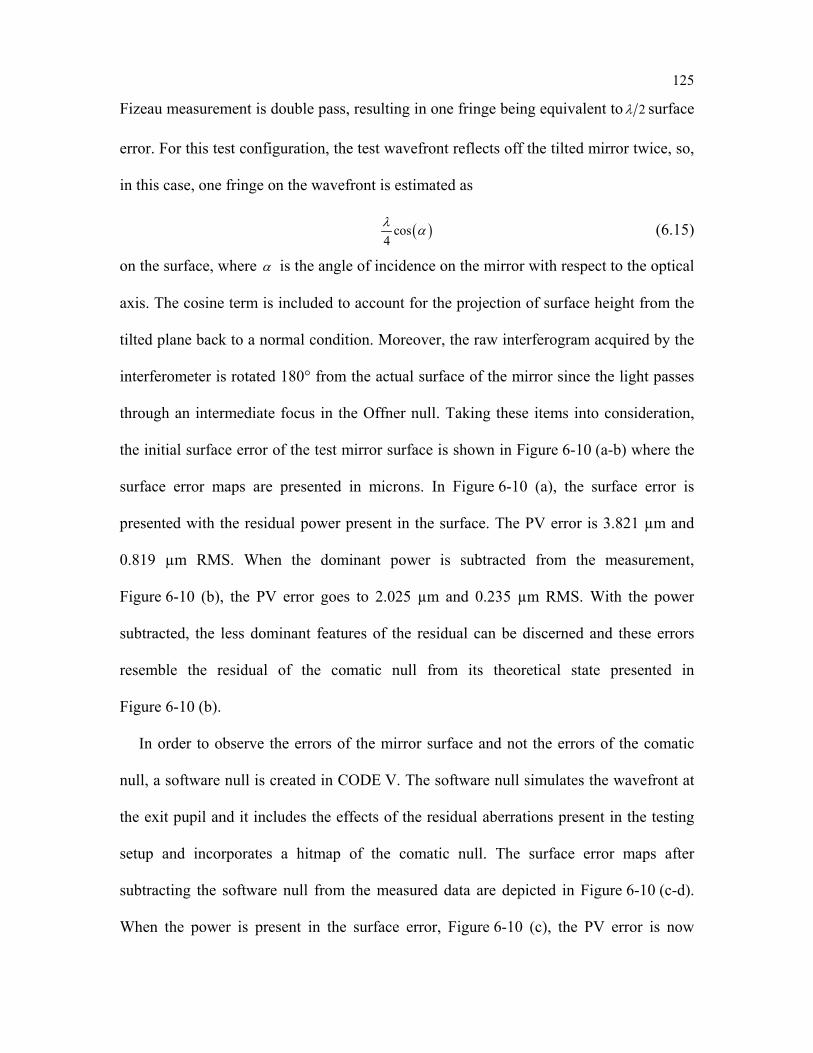
125
Fizeau measurement is double pass, resulting in one fringe being equivalent to 2λ surface
error. For this test configuration, the test wavefront reflects off the tilted mirror twice, so,
in this case, one fringe on the wavefront is estimated as
( )cos4λ α (6.15)
on the surface, where α is the angle of incidence on the mirror with respect to the optical
axis. The cosine term is included to account for the projection of surface height from the
tilted plane back to a normal condition. Moreover, the raw interferogram acquired by the
interferometer is rotated 180° from the actual surface of the mirror since the light passes
through an intermediate focus in the Offner null. Taking these items into consideration,
the initial surface error of the test mirror surface is shown in Figure 6-10 (a-b) where the
surface error maps are presented in microns. In Figure 6-10 (a), the surface error is
presented with the residual power present in the surface. The PV error is 3.821 µm and
0.819 µm RMS. When the dominant power is subtracted from the measurement,
Figure 6-10 (b), the PV error goes to 2.025 µm and 0.235 µm RMS. With the power
subtracted, the less dominant features of the residual can be discerned and these errors
resemble the residual of the comatic null from its theoretical state presented in
Figure 6-10 (b).
In order to observe the errors of the mirror surface and not the errors of the comatic
null, a software null is created in CODE V. The software null simulates the wavefront at
the exit pupil and it includes the effects of the residual aberrations present in the testing
setup and incorporates a hitmap of the comatic null. The surface error maps after
subtracting the software null from the measured data are depicted in Figure 6-10 (c-d).
When the power is present in the surface error, Figure 6-10 (c), the PV error is now
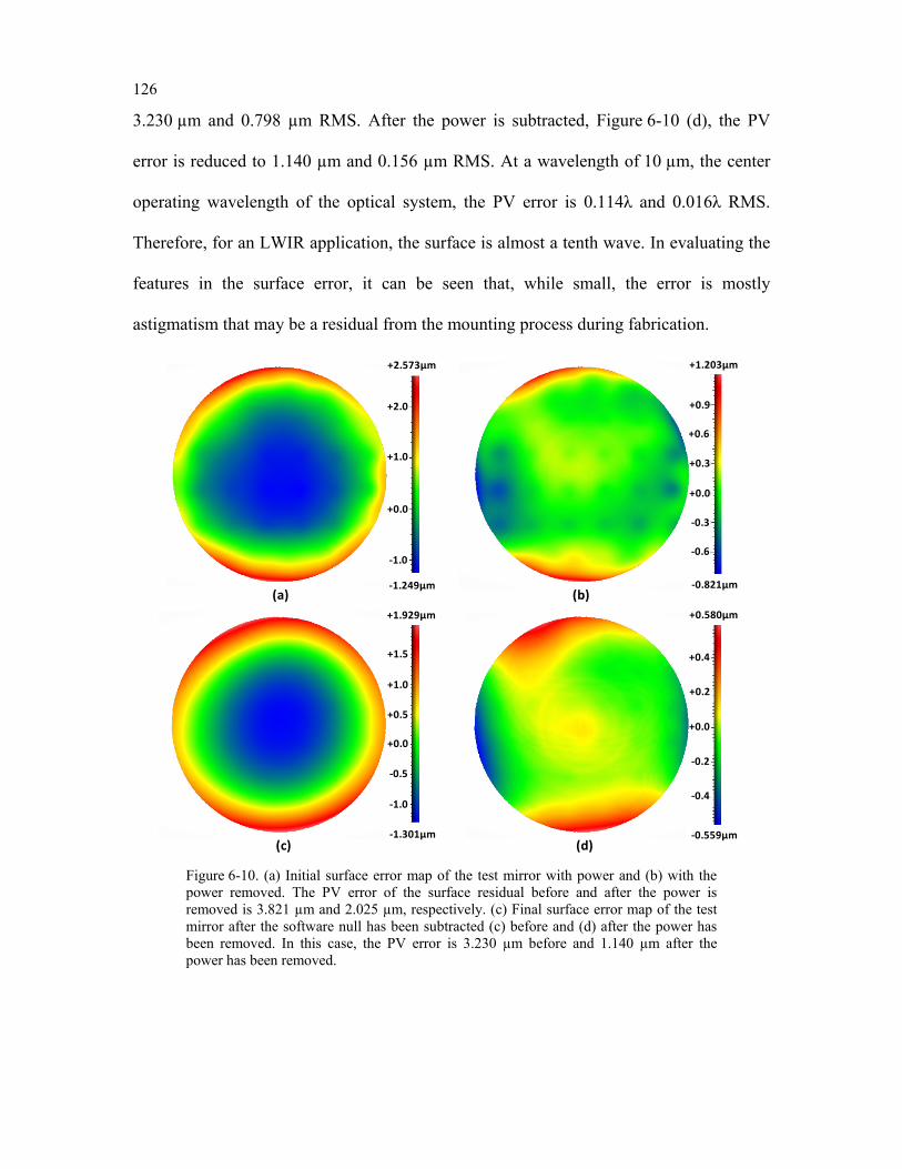
126
3.230 µm and 0.798 µm RMS. After the power is subtracted, Figure 6-10 (d), the PV
error is reduced to 1.140 µm and 0.156 µm RMS. At a wavelength of 10 µm, the center
operating wavelength of the optical system, the PV error is 0.114λ and 0.016λ RMS.
Therefore, for an LWIR application, the surface is almost a tenth wave. In evaluating the
features in the surface error, it can be seen that, while small, the error is mostly
astigmatism that may be a residual from the mounting process during fabrication.
(c) (d)
(a) (b)
-0.559µm
+0.580µm
+0.0
-0.4
-0.2
+0.2
+0.4
+2.573µm
-1.249µm
-1.0
+0.0
+1.0
+2.0
-1.301µm
+0.5
-0.5
+0.0
+1.0
+1.5
-1.0
+1.929µm
-0.821µm
+0.3
-0.3
+0.0
+0.6
+0.9
-0.6
+1.203µm
Figure 6-10. (a) Initial surface error map of the test mirror with power and (b) with the power removed. The PV error of the surface residual before and after the power is removed is 3.821 µm and 2.025 µm, respectively. (c) Final surface error map of the test mirror after the software null has been subtracted (c) before and (d) after the power has been removed. In this case, the PV error is 3.230 µm before and 1.140 µm after the power has been removed.
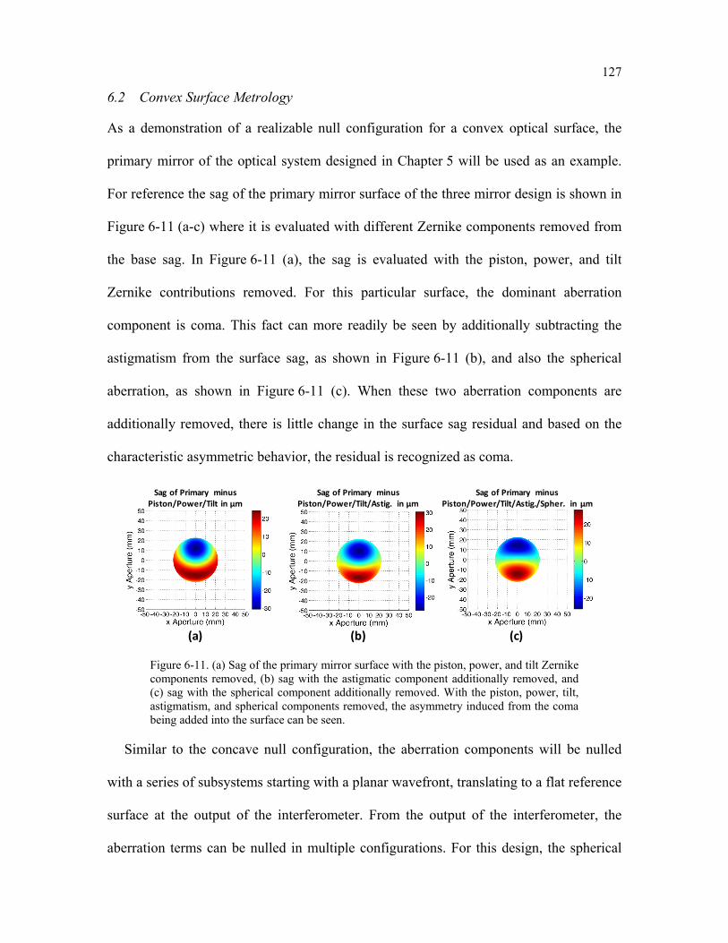
127
6.2 Convex Surface Metrology
As a demonstration of a realizable null configuration for a convex optical surface, the
primary mirror of the optical system designed in Chapter 5 will be used as an example.
For reference the sag of the primary mirror surface of the three mirror design is shown in
Figure 6-11 (a-c) where it is evaluated with different Zernike components removed from
the base sag. In Figure 6-11 (a), the sag is evaluated with the piston, power, and tilt
Zernike contributions removed. For this particular surface, the dominant aberration
component is coma. This fact can more readily be seen by additionally subtracting the
astigmatism from the surface sag, as shown in Figure 6-11 (b), and also the spherical
aberration, as shown in Figure 6-11 (c). When these two aberration components are
additionally removed, there is little change in the surface sag residual and based on the
characteristic asymmetric behavior, the residual is recognized as coma.
(a) (b) (c)
Sag of Primary minus Piston/Power/Tilt in µm
Sag of Primary minus Piston/Power/Tilt/Astig. in µm
Sag of Primary minus Piston/Power/Tilt/Astig./Spher. in µm
Figure 6-11. (a) Sag of the primary mirror surface with the piston, power, and tilt Zernike components removed, (b) sag with the astigmatic component additionally removed, and (c) sag with the spherical component additionally removed. With the piston, power, tilt, astigmatism, and spherical components removed, the asymmetry induced from the coma being added into the surface can be seen.
Similar to the concave null configuration, the aberration components will be nulled
with a series of subsystems starting with a planar wavefront, translating to a flat reference
surface at the output of the interferometer. From the output of the interferometer, the
aberration terms can be nulled in multiple configurations. For this design, the spherical
128
aberration component is first nulled by the use of an afocal, refractive Offner null,
consisting of two refractive elements, one of which is a null lens that introduces the
opposite amount of spherical aberration present in the mirror under test and the other is a
field lens that collimates the beam and conjugates the null lens to the mirror under test.
Next, the astigmatic component is removed by operating the mirror off-axis, or tilting the
mirror. Unlike for the case of a concave test mirror where the wavefront converges to a
point, the beam exiting the tilted, convex mirror will diverge so an additional auxiliary
optic is needed to focus the wavefront. In this case, a large concave mirror is used similar
to a Hindle sphere [81]. This additional mirror adds another DOF so that its tilt is used to
remove the residual comatic contribution present in the wavefront. Finally, similar to the
concave null configuration, the residual higher order terms are nulled by adding their
opposite departure on a DM that also acts as a reimaging retro-reflector to send the light
back towards the measurement interferometer. In order to couple the wavefront to the
quasi-flat DM, the wavefront is collimated with the use of an additional lens. Together
these three components form a configuration that allows the optical surface to be
measured with a conventional interferometer.
The sizing of the various optical components constrains the layout of the
interferometric null. The region of interest on the test mirror is 45 mm in diameter while
the output from the Zygo interferometer is 101.6 mm. To keep the components of the
refractive null readily commercially available, a 1:1 afocal Offner null is selected so only
45 mm of the 101.6 mm aperture is used. After the wavefront passes through the null lens
and reflects off the test mirror, its beam size will grow rapidly as the wavefront is
diverging. As a result, the distance between the test mirror and auxiliary mirror should be
129
minimized to keep the beam footprint on the auxiliary mirror small. The auxiliary mirror
clear aperture and its beam footprint are constrained to 150 mm diameter maximum,
which is the largest mirror size that is readily commercially available at relatively fast
focal ratios. The focal ratio must be fast to keep the length of the null small. An F/1,
150 mm COTS sphere is used to meet these constraints. The distance between the
auxiliary sphere and the mirror under test also impacts how the wavefront traverses
through the entire null configuration. The beam exiting the afocal Offner null must pass
by the auxiliary sphere and the sphere should not obscure the incoming beam. Similarly,
after the beam has reflected off the auxiliary sphere, it passes by the mirror under test and
the mirror should not obscure the beam either. The distance between the test and
auxiliary mirror is set so that when the two mirrors are tilted to null both astigmatism and
coma, they do not obscure any part of the beam. Lastly, the DM has a 15 mm clear
aperture so the collimating lens after the auxiliary sphere must be arranged to meet this
constraint. With all these constraints in mind, a solution is optimized in CODE V with
user defined constraints to null the Fringe Zernike spherical aberration, astigmatism,
coma, and any higher order aberration terms while ensuring that the clear aperture
limitations are met, the beam is not obscured, and the imaging conjugates between
components are maintained.
The final, optimized system is shown in the YZ plane in Figure 6-12. The overall
package of the interferometric null is roughly 700 mm x 350 mm. All the lens
components are plano-convex making them readily commercially available. The
theoretical interferogram exiting the interferometric null is shown in Figure 6-13 (a)
before the DM is active and in Figure 6-13 (b) after the higher order null has been
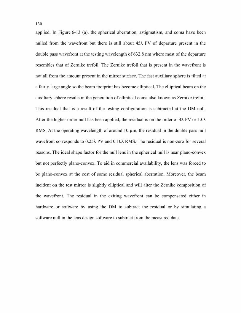
130
applied. In Figure 6-13 (a), the spherical aberration, astigmatism, and coma have been
nulled from the wavefront but there is still about 45λ PV of departure present in the
double pass wavefront at the testing wavelength of 632.8 nm where most of the departure
resembles that of Zernike trefoil. The Zernike trefoil that is present in the wavefront is
not all from the amount present in the mirror surface. The fast auxiliary sphere is tilted at
a fairly large angle so the beam footprint has become elliptical. The elliptical beam on the
auxiliary sphere results in the generation of elliptical coma also known as Zernike trefoil.
This residual that is a result of the testing configuration is subtracted at the DM null.
After the higher order null has been applied, the residual is on the order of 4λ PV or 1.0λ
RMS. At the operating wavelength of around 10 µm, the residual in the double pass null
wavefront corresponds to 0.25λ PV and 0.10λ RMS. The residual is non-zero for several
reasons. The ideal shape factor for the null lens in the spherical null is near plano-convex
but not perfectly plano-convex. To aid in commercial availability, the lens was forced to
be plano-convex at the cost of some residual spherical aberration. Moreover, the beam
incident on the test mirror is slightly elliptical and will alter the Zernike composition of
the wavefront. The residual in the exiting wavefront can be compensated either in
hardware or software by using the DM to subtract the residual or by simulating a
software null in the lens design software to subtract from the measured data.
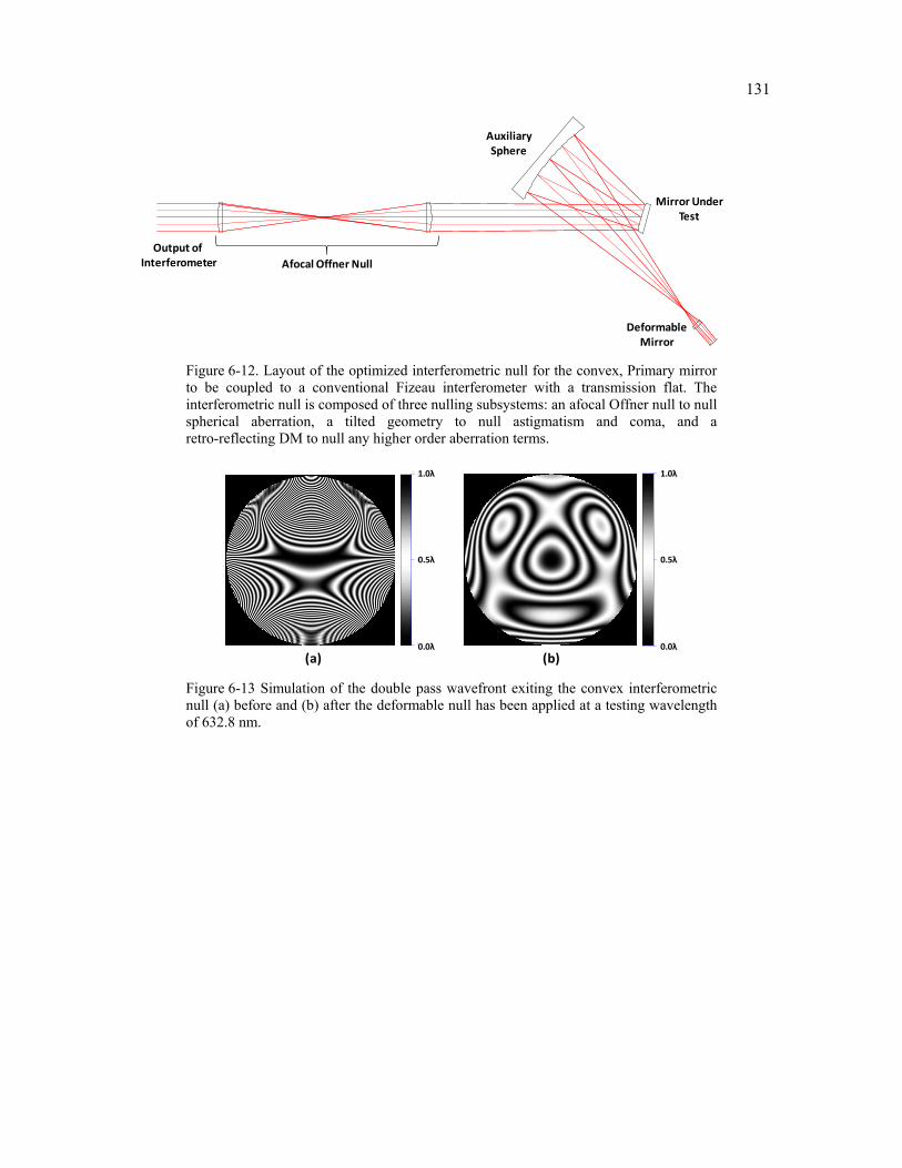
131
Afocal Offner Null
DeformableMirror
Mirror UnderTest
Auxiliary Sphere
Output of Interferometer
Figure 6-12. Layout of the optimized interferometric null for the convex, Primary mirror to be coupled to a conventional Fizeau interferometer with a transmission flat. The interferometric null is composed of three nulling subsystems: an afocal Offner null to null spherical aberration, a tilted geometry to null astigmatism and coma, and a retro-reflecting DM to null any higher order aberration terms.
0.0λ
0.5λ
1.0λ
a e
0
1
0
0.0λ
0.5λ
1.0λ
(a) (b)
Figure 6-13 Simulation of the double pass wavefront exiting the convex interferometric null (a) before and (b) after the deformable null has been applied at a testing wavelength of 632.8 nm.
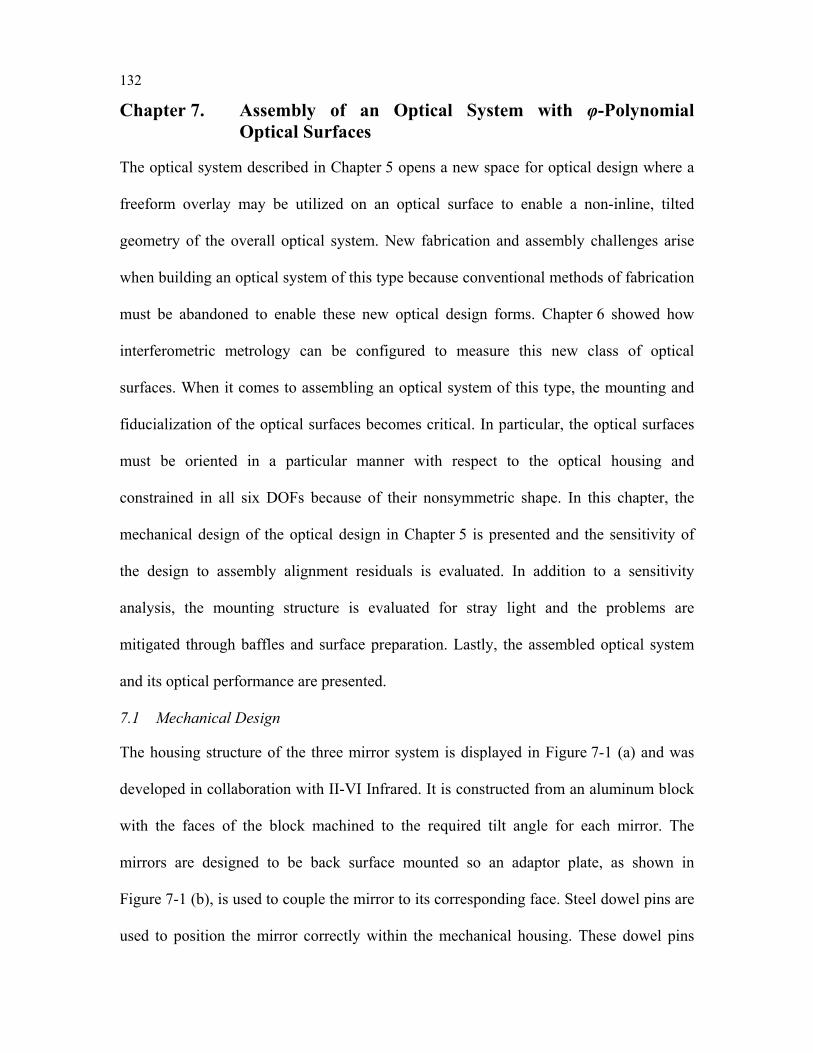
132
Chapter 7. Assembly of an Optical System with φ-Polynomial Optical Surfaces
The optical system described in Chapter 5 opens a new space for optical design where a
freeform overlay may be utilized on an optical surface to enable a non-inline, tilted
geometry of the overall optical system. New fabrication and assembly challenges arise
when building an optical system of this type because conventional methods of fabrication
must be abandoned to enable these new optical design forms. Chapter 6 showed how
interferometric metrology can be configured to measure this new class of optical
surfaces. When it comes to assembling an optical system of this type, the mounting and
fiducialization of the optical surfaces becomes critical. In particular, the optical surfaces
must be oriented in a particular manner with respect to the optical housing and
constrained in all six DOFs because of their nonsymmetric shape. In this chapter, the
mechanical design of the optical design in Chapter 5 is presented and the sensitivity of
the design to assembly alignment residuals is evaluated. In addition to a sensitivity
analysis, the mounting structure is evaluated for stray light and the problems are
mitigated through baffles and surface preparation. Lastly, the assembled optical system
and its optical performance are presented.
7.1 Mechanical Design
The housing structure of the three mirror system is displayed in Figure 7-1 (a) and was
developed in collaboration with II-VI Infrared. It is constructed from an aluminum block
with the faces of the block machined to the required tilt angle for each mirror. The
mirrors are designed to be back surface mounted so an adaptor plate, as shown in
Figure 7-1 (b), is used to couple the mirror to its corresponding face. Steel dowel pins are
used to position the mirror correctly within the mechanical housing. These dowel pins
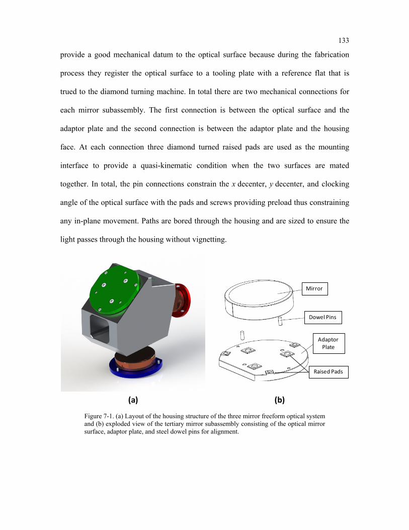
133
provide a good mechanical datum to the optical surface because during the fabrication
process they register the optical surface to a tooling plate with a reference flat that is
trued to the diamond turning machine. In total there are two mechanical connections for
each mirror subassembly. The first connection is between the optical surface and the
adaptor plate and the second connection is between the adaptor plate and the housing
face. At each connection three diamond turned raised pads are used as the mounting
interface to provide a quasi-kinematic condition when the two surfaces are mated
together. In total, the pin connections constrain the x decenter, y decenter, and clocking
angle of the optical surface with the pads and screws providing preload thus constraining
any in-plane movement. Paths are bored through the housing and are sized to ensure the
light passes through the housing without vignetting.
Mirror
Dowel Pins
Adaptor Plate
(a) (b)
Raised Pads
Figure 7-1. (a) Layout of the housing structure of the three mirror freeform optical system and (b) exploded view of the tertiary mirror subassembly consisting of the optical mirror surface, adaptor plate, and steel dowel pins for alignment.
134
7.1.1 Sensitivity Analysis
As is the case with any piece of hardware, there is some tolerance on how well the
mirrors can be positioned in the housing relative to their nominal value. The key is to
ensure that within the manufacturing tolerances, the as-built optical system remains
diffraction limited. In addition to hardware tolerances, the assembly method of the optical
system may impact the manufacturing tolerances. If the optical system is to be passively
aligned, that is, no adjustments are made with the exception of focus, the manufacturing
tolerances will have to be tighter. If the system is to be actively aligned, that is, a
compensator is used to restore the optical performance during assembly, the assessment
of the performance during alignment is important and the mechanical complexity of the
housing will have to increase because a DOF must now be made adjustable. In this
section, both approaches are explored.
7.1.1.1 Passive Alignment
In a passive alignment approach, the three mirrors must be constrained in their x/y
translation, tip/tilt, and clocking angle. There are also two vertex spacings that must be
held between the three mirrors. The spacing between the tertiary mirror and focal plane is
used as a focus adjustment after assembly. The focus compensation is performed by
shimming the detector in 12.5 µm steps and determining through an optical assessment
the shim that provides the best performance. The detector must also be held in tip and tilt
relative to the housing and there is a separate tip and tilt tolerance for the focal plane
relative to the mounting fixtures on the detector. In total, there are 21 positioning
tolerances to consider for this assembly.
To check the sensitivity of the optical housing to manufacturing errors, each tolerance
is perturbed by its expected error value and the change in the RMS WFE after focus
135
compensation is recorded for several field points. Once each tolerance and its resulting
change in performance is computed, the total change in performance for each field is
computed as the root sum square (RSS) of all the tolerances. The results of this analysis
are displayed in Table 7-1 where the change in RMS WFE is displayed for each tolerance
at two field points: on-axis (0°, 0°) and the most sensitive field (4°, 3°). For this analysis
the x decenter, y decenter, and despace of the mirrors is assumed to be ±50 µm, the tip
and tilt of the mirrors and detector (α and β tilt) is assumed to be ±1 arc min or ±0.017°,
and the clocking angle (γ rotation) is assumed to be larger at ±0.1°. From the mechanical
drawing of the detector, the focal plane tip and tilt tolerances are calculated to be roughly
±0.56°. With all the tolerances considered, the as-built RMS WFE is found to be roughly
0.056λ for the (0°, 0°) field and 0.060λ for the (4°, 3°) field, both of which are within the
diffraction limit of 0.07λ. Looking at the tolerances on a term by term basis, the primary
contributors to the overall loss in performance are the tilt tolerances on the secondary
mirror, tertiary mirror, and focal plane. Therefore, the initial tolerances selected are
sufficient for meeting the performance specification; however, they do not consider how
the optical components will actually be mated together. Since the components are to be
assembled with pin connections, an alternative analysis would be to model the sensitivity
of the connections directly. The position of the dowel pin holes affects the x decenter,
y decenter, and clocking angle of the mirror surfaces.
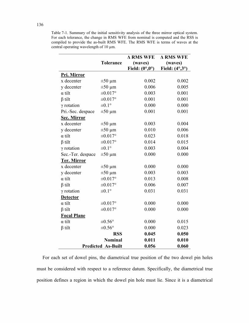
136
Table 7-1. Summary of the initial sensitivity analysis of the three mirror optical system. For each tolerance, the change in RMS WFE from nominal is computed and the RSS is compiled to provide the as-built RMS WFE. The RMS WFE is terms of waves at the central operating wavelength of 10 µm.
Tolerance Δ RMS WFE
(waves) Field: (0°,0°)
Δ RMS WFE (waves)
Field: (4°,3°) Pri. Mirror x decenter ±50 µm 0.002 0.002 y decenter ±50 µm 0.006 0.005 α tilt ±0.017° 0.003 0.001 β tilt ±0.017° 0.001 0.001 γ rotation ±0.1° 0.000 0.000 Pri.-Sec. despace ±50 µm 0.001 0.001 Sec. Mirror x decenter ±50 µm 0.003 0.004 y decenter ±50 µm 0.010 0.006 α tilt ±0.017° 0.023 0.018 β tilt ±0.017° 0.014 0.015 γ rotation ±0.1° 0.003 0.004 Sec.-Ter. despace ±50 µm 0.000 0.000 Ter. Mirror x decenter ±50 µm 0.000 0.000 y decenter ±50 µm 0.003 0.003 α tilt ±0.017° 0.013 0.008 β tilt ±0.017° 0.006 0.007 γ rotation ±0.1° 0.031 0.031 Detector α tilt ±0.017° 0.000 0.000 β tilt ±0.017° 0.000 0.000 Focal Plane α tilt ±0.56° 0.000 0.015 β tilt ±0.56° 0.000 0.023
RSS 0.045 0.050 Nominal 0.011 0.010
Predicted As-Built 0.056 0.060
For each set of dowel pins, the diametrical true position of the two dowel pin holes
must be considered with respect to a reference datum. Specifically, the diametrical true
position defines a region in which the dowel pin hole must lie. Since it is a diametrical
137
tolerance zone, as the x decenter of the dowel pin hole increases, the y decenter must
decrease accordingly. Furthermore, if the top dowel pin hole is not collinear with the
bottom dowel pin hole, the mirror will be rotated.
For the analysis, an initial diametrical true position tolerance, φ , is selected for the
position of the top and bottom dowel pin holes. From this tolerance a random x decenter
of the hole is selected from a position within the tolerance zone, computed as
( )/ 2 ,2 2
T Bdecx RANDφ φ
= − + (7.1)
where /T Bdecx is the x decenter of either the top or bottom hole and RAND is a normally
distributed random number between 0 and 1. From the x decenter, the maximum possible
y decenter, /maxT B
decy , is calculated as
( )2
2/ /max .
2T B T B
dec decy xφ = −
(7.2)
From Eq. (7.2) a random y decenter of either the top or bottom hole is computed as
( )/ / /max max2 .T B T B T B
dec dec decy y RAND y= − + (7.3)
With the x and y decenter computed for both the top and bottom dowel pin holes, the total
x and y decenter of the set is computed as
,2
T Bdec dec
decx x
x+
= (7.4)
and
.2
T Bdec dec
decy y
y+
= (7.5)
Lastly, the clocking angle error of the set, γ , is computed as
1tan ,T Bdec dec
pin
x xd
γ − −
=
(7.6)
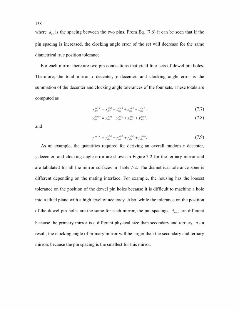
138
where pind is the spacing between the two pins. From Eq. (7.6) it can be seen that if the
pin spacing is increased, the clocking angle error of the set will decrease for the same
diametrical true position tolerance.
For each mirror there are two pin connections that yield four sets of dowel pin holes.
Therefore, the total mirror x decenter, y decenter, and clocking angle error is the
summation of the decenter and clocking angle tolerances of the four sets. These totals are
computed as
1 2 3 4 ,mirror pin pin pin pindec dec dec dec decx x x x x= + + + (7.7)
1 2 3 4 ,mirror pin pin pin pindec dec dec dec decy y y y y= + + + (7.8)
and
1 2 3 4 .mirror pin pin pin pindec dec dec decγ γ γ γ γ= + + + (7.9)
As an example, the quantities required for deriving an overall random x decenter,
y decenter, and clocking angle error are shown in Figure 7-2 for the tertiary mirror and
are tabulated for all the mirror surfaces in Table 7-2. The diametrical tolerance zone is
different depending on the mating interface. For example, the housing has the loosest
tolerance on the position of the dowel pin holes because it is difficult to machine a hole
into a tilted plane with a high level of accuracy. Also, while the tolerance on the position
of the dowel pin holes are the same for each mirror, the pin spacings, pind , are different
because the primary mirror is a different physical size than secondary and tertiary. As a
result, the clocking angle of primary mirror will be larger than the secondary and tertiary
mirrors because the pin spacing is the smallest for this mirror.
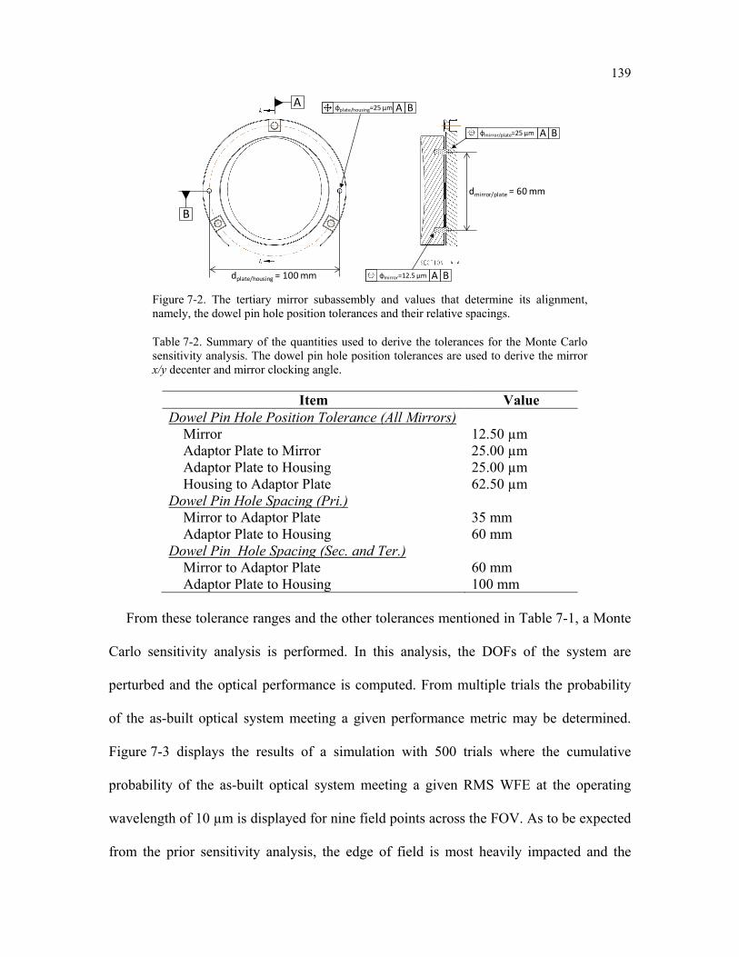
139
dplate/housing = 100 mm
dmirror/plate = 60 mm
A
B
φplate/housing=25 µm A B
φmirror/plate=25 µm A B
φmirror=12.5 µm A B
Figure 7-2. The tertiary mirror subassembly and values that determine its alignment, namely, the dowel pin hole position tolerances and their relative spacings.
Table 7-2. Summary of the quantities used to derive the tolerances for the Monte Carlo sensitivity analysis. The dowel pin hole position tolerances are used to derive the mirror x/y decenter and mirror clocking angle.
Item Value Dowel Pin Hole Position Tolerance (All Mirrors)
Mirror 12.50 µm Adaptor Plate to Mirror 25.00 µm Adaptor Plate to Housing 25.00 µm Housing to Adaptor Plate 62.50 µm
Dowel Pin Hole Spacing (Pri.) Mirror to Adaptor Plate 35 mm Adaptor Plate to Housing 60 mm
Dowel Pin Hole Spacing (Sec. and Ter.) Mirror to Adaptor Plate 60 mm Adaptor Plate to Housing 100 mm
From these tolerance ranges and the other tolerances mentioned in Table 7-1, a Monte
Carlo sensitivity analysis is performed. In this analysis, the DOFs of the system are
perturbed and the optical performance is computed. From multiple trials the probability
of the as-built optical system meeting a given performance metric may be determined.
Figure 7-3 displays the results of a simulation with 500 trials where the cumulative
probability of the as-built optical system meeting a given RMS WFE at the operating
wavelength of 10 µm is displayed for nine field points across the FOV. As to be expected
from the prior sensitivity analysis, the edge of field is most heavily impacted and the
140
change in performance is most likely dominated by the large focal plane tilt tolerance. If
a cumulative 95% is selected as the passing metric, all the field points lie below an
as-built RMS WFE of 0.06λ. These results are in good agreement with the prior analysis
where the as-built performance was around 0.06λ. From these two analyses, it can be
concluded that the optical system can be machined and assembled with standard machine
shop tolerances and the final system will remain diffraction limited, less than 0.07λ,
throughout the FOV.
0%
20%
40%
60%
80%
100%
0 0.01 0.02 0.03 0.04 0.05 0.06 0.07
Cum
ulat
ive P
erce
ntag
e
As-Built RMS Wavefront Error (waves at 10µm)
(+0°,+0°)
(-4°,+0°)
(+4°,+0°)
(-3°,+0°)
(+3°,+0°)
(+4°,+3°)
(+4°,-3°)
(-4°,+3°)
(-4°,-3°)
Figure 7-3. Cumulative probability as a function of as-built RMS WFE for the three mirror optical system over nine field points assuming only passive alignment.
7.1.1.2 Active Alignment
The two analyses performed in section 7.1.1.1 assumed that the optical system is to be
passively aligned where the as-built optical performance is determined by the as-built
manufacturing tolerances and a shim for focus compensation. If now some additional
DOFs are allowed to vary during the assembly process, it may be possible to improve the
as-built optical performance. Active alignment becomes more likely as the optical design
form is considered for shorter wavebands.
141
The previously shown sensitivity analyses use the overall RMS WFE as the
performance metric to assess the as-built optical performance; however, it does not
provide any information on which aberration contributions are limiting the performance
and how they vary throughout the FOV. If the DOFs are perturbed a known amount and
now the Zernike aberration contributions are monitored throughout the FOV using the
FFD, additional insight can be gathered on alignment strategies as well as which DOFs
are going to be best for compensators. From the results of the sensitivity analysis in
Table 7-1, it is seen that for the optical system, in general, there is a greater loss in
performance when the mirror components are tilted versus decentered, so an effective
compensator will be the mirror tilt. Figure 7-4 (a-d) displays the FFDs for Zernike
astigmatism (Z5/6) and Zernike coma (Z7/8) for the nominal optical system, shown in
Figure 7-4 (a), and for the case where the mirrors are individually tilted +0.1° in the YZ
plane, shown in Figure 7-4 (b-d). When each mirror is tilted, the primary aberration
component induced is field constant astigmatism. Some field constant coma is induced as
well; though, its magnitude is about ten times less than that of the astigmatism.
From this result, several conclusions can be drawn. First, since field constant
astigmatism is primarily induced when the telescope is misaligned, during active
alignment only one field point needs to be monitored to get a good representation of how
the other field points are behaving. Second, for the same tilt of the three mirrors, the
secondary is most sensitive to the perturbation. Consequently, this mirror may make the
most effective compensator because a small perturbation of the mirror will have a large
net effect on the overall system performance, thus requiring less mechanical movement
of the compensator, assuming the compensator has enough mechanical resolution. The
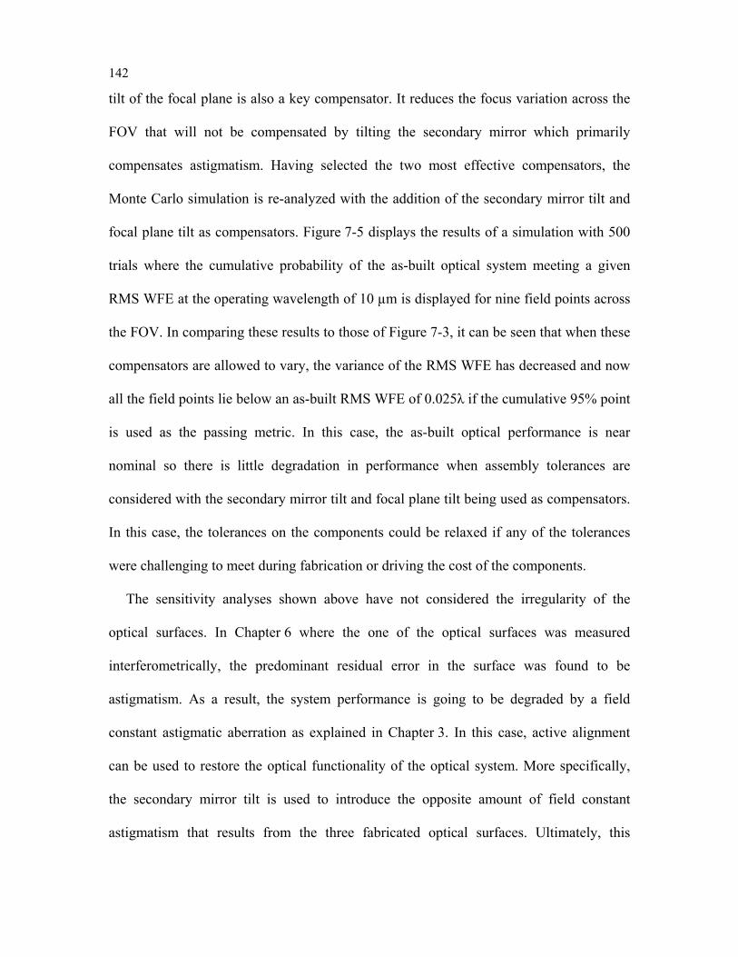
142
tilt of the focal plane is also a key compensator. It reduces the focus variation across the
FOV that will not be compensated by tilting the secondary mirror which primarily
compensates astigmatism. Having selected the two most effective compensators, the
Monte Carlo simulation is re-analyzed with the addition of the secondary mirror tilt and
focal plane tilt as compensators. Figure 7-5 displays the results of a simulation with 500
trials where the cumulative probability of the as-built optical system meeting a given
RMS WFE at the operating wavelength of 10 µm is displayed for nine field points across
the FOV. In comparing these results to those of Figure 7-3, it can be seen that when these
compensators are allowed to vary, the variance of the RMS WFE has decreased and now
all the field points lie below an as-built RMS WFE of 0.025λ if the cumulative 95% point
is used as the passing metric. In this case, the as-built optical performance is near
nominal so there is little degradation in performance when assembly tolerances are
considered with the secondary mirror tilt and focal plane tilt being used as compensators.
In this case, the tolerances on the components could be relaxed if any of the tolerances
were challenging to meet during fabrication or driving the cost of the components.
The sensitivity analyses shown above have not considered the irregularity of the
optical surfaces. In Chapter 6 where the one of the optical surfaces was measured
interferometrically, the predominant residual error in the surface was found to be
astigmatism. As a result, the system performance is going to be degraded by a field
constant astigmatic aberration as explained in Chapter 3. In this case, active alignment
can be used to restore the optical functionality of the optical system. More specifically,
the secondary mirror tilt is used to introduce the opposite amount of field constant
astigmatism that results from the three fabricated optical surfaces. Ultimately, this
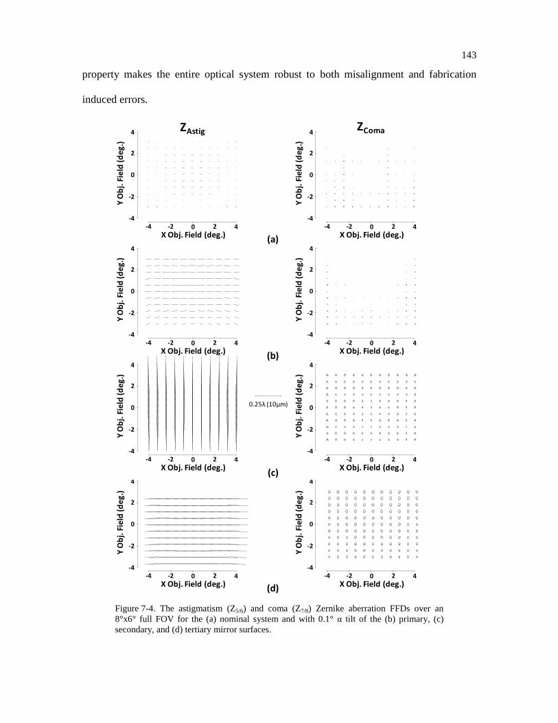
143
property makes the entire optical system robust to both misalignment and fabrication
induced errors.
16:04:40
Zernike Polynomial
KHF 01-Nov-13
FRINGE ZERNIKE PAIR Z5 AND Z6
vs
FIELD ANGLE IN OBJECT SPACE
Minimum = 0.15967
Maximum = 0.21519
Average = 0.19827
Std Dev = 0.013871
0.25waves (10600.0 nm)
-6 -4 -2 0 2 4 6
X Field Angle in Object Space - degrees
-6
-4
-2
0
2
4
6
Y Field Angle in Object Space - degrees
16:04:41
Zernike Polynomial
KHF 01-Nov-13
FRINGE ZERNIKE PAIR Z7 AND Z8
vs
FIELD ANGLE IN OBJECT SPACE
Minimum = 0.020385
Maximum = 0.033847
Average = 0.028041
Std Dev = 0.0033958
0.25waves (10600.0 nm)
-6 -4 -2 0 2 4 6
X Field Angle in Object Space - degrees
-6
-4
-2
0
2
4
6
Y Field Angle in Object Space - degrees
15:15:47
Zernike Polynomial
KHF 01-Nov-13
FRINGE ZERNIKE PAIR Z5 AND Z6
vs
FIELD ANGLE IN OBJECT SPACE
Minimum = 0.00097077
Maximum = 0.026129
Average = 0.011091
Std Dev = 0.0056026
0.25waves (10600.0 nm)
-6 -4 -2 0 2 4 6
X Field Angle in Object Space - degrees
-6
-4
-2
0
2
4
6
Y Field Angle in Object Space - degrees
X Obj. Field (deg.)-4 -2 0 2 4
4
0
2
-2
-4
Y O
bj.
Fie
ld (d
eg.
)
15:15:47
Zernike Polynomial
KHF 01-Nov-13
FRINGE ZERNIKE PAIR Z5 AND Z6
vs
FIELD ANGLE IN OBJECT SPACE
Minimum = 0.00097077
Maximum = 0.026129
Average = 0.011091
Std Dev = 0.0056026
0.25waves (10600.0 nm)
-6 -4 -2 0 2 4 6
X Field Angle in Object Space - degrees
-6
-4
-2
0
2
4
6
Y Field Angle in Object Space - degrees
X Obj. Field (deg.)-4 -2 0 2 4
4
0
2
-2
-4
Y O
bj.
Fie
ld (d
eg.
)
16:03:10
Zernike Polynomial
KHF 01-Nov-13
FRINGE ZERNIKE PAIR Z5 AND Z6
vs
FIELD ANGLE IN OBJECT SPACE
Minimum = 0.30753
Maximum = 0.39565
Average = 0.33898
Std Dev = 0.024489
0.25waves (10600.0 nm)
-6 -4 -2 0 2 4 6
X Field Angle in Object Space - degrees
-6
-4
-2
0
2
4
6
Y Field Angle in Object Space - degrees
16:04:02
Zernike Polynomial
KHF 01-Nov-13
FRINGE ZERNIKE PAIR Z7 AND Z8
vs
FIELD ANGLE IN OBJECT SPACE
Minimum = 0.01667
Maximum = 0.022854
Average = 0.019084
Std Dev = 0.001515
0.25waves (10600.0 nm)
-6 -4 -2 0 2 4 6
X Field Angle in Object Space - degrees
-6
-4
-2
0
2
4
6
Y Field Angle in Object Space - degrees
15:15:47
Zernike Polynomial
KHF 01-Nov-13
FRINGE ZERNIKE PAIR Z5 AND Z6
vs
FIELD ANGLE IN OBJECT SPACE
Minimum = 0.00097077
Maximum = 0.026129
Average = 0.011091
Std Dev = 0.0056026
0.25waves (10600.0 nm)
-6 -4 -2 0 2 4 6
X Field Angle in Object Space - degrees
-6
-4
-2
0
2
4
6
Y Field Angle in Object Space - degrees
X Obj. Field (deg.)-4 -2 0 2 4
4
0
2
-2
-4
Y O
bj.
Fie
ld (d
eg.
)
15:15:47
Zernike Polynomial
KHF 01-Nov-13
FRINGE ZERNIKE PAIR Z5 AND Z6
vs
FIELD ANGLE IN OBJECT SPACE
Minimum = 0.00097077
Maximum = 0.026129
Average = 0.011091
Std Dev = 0.0056026
0.25waves (10600.0 nm)
-6 -4 -2 0 2 4 6
X Field Angle in Object Space - degrees
-6
-4
-2
0
2
4
6
Y Field Angle in Object Space - degrees
X Obj. Field (deg.)-4 -2 0 2 4
4
0
2
-2
-4
Y O
bj.
Fie
ld (d
eg.
)
15:58:49
Zernike Polynomial
KHF 01-Nov-13
FRINGE ZERNIKE PAIR Z5 AND Z6
vs
FIELD ANGLE IN OBJECT SPACE
Minimum = 0.036542
Maximum = 0.07623
Average = 0.060924
Std Dev = 0.01086
0.25waves (10600.0 nm)
-6 -4 -2 0 2 4 6
X Field Angle in Object Space - degrees
-6
-4
-2
0
2
4
6
Y Field Angle in Object Space - degrees
15:59:05
Zernike Polynomial
KHF 01-Nov-13
FRINGE ZERNIKE PAIR Z7 AND Z8
vs
FIELD ANGLE IN OBJECT SPACE
Minimum = 0.00016152
Maximum = 0.0089318
Average = 0.003117
Std Dev = 0.0021271
0.25waves (10600.0 nm)
-6 -4 -2 0 2 4 6
X Field Angle in Object Space - degrees
-6
-4
-2
0
2
4
6
Y Field Angle in Object Space - degrees
15:15:47
Zernike Polynomial
KHF 01-Nov-13
FRINGE ZERNIKE PAIR Z5 AND Z6
vs
FIELD ANGLE IN OBJECT SPACE
Minimum = 0.00097077
Maximum = 0.026129
Average = 0.011091
Std Dev = 0.0056026
0.25waves (10600.0 nm)
-6 -4 -2 0 2 4 6
X Field Angle in Object Space - degrees
-6
-4
-2
0
2
4
6
Y Field Angle in Object Space - degrees
X Obj. Field (deg.)-4 -2 0 2 4
4
0
2
-2
-4
Y O
bj.
Fie
ld (d
eg.)
15:15:47
Zernike Polynomial
KHF 01-Nov-13
FRINGE ZERNIKE PAIR Z5 AND Z6
vs
FIELD ANGLE IN OBJECT SPACE
Minimum = 0.00097077
Maximum = 0.026129
Average = 0.011091
Std Dev = 0.0056026
0.25waves (10600.0 nm)
-6 -4 -2 0 2 4 6
X Field Angle in Object Space - degrees
-6
-4
-2
0
2
4
6
Y Field Angle in Object Space - degrees
X Obj. Field (deg.)-4 -2 0 2 4
4
0
2
-2
-4
Y O
bj.
Fie
ld (d
eg.)
15:15:47
Zernike Polynomial
KHF 01-Nov-13
FRINGE ZERNIKE PAIR Z5 AND Z6
vs
FIELD ANGLE IN OBJECT SPACE
Minimum = 0.00097077
Maximum = 0.026129
Average = 0.011091
Std Dev = 0.0056026
0.25waves (10600.0 nm)
-6 -4 -2 0 2 4 6
X Field Angle in Object Space - degrees
-6
-4
-2
0
2
4
6
Y Field Angle in Object Space - degrees
14:44:01
Zernike Polynomial
KHF 01-Nov-13
FRINGE ZERNIKE PAIR Z7 AND Z8
vs
FIELD ANGLE IN OBJECT SPACE
Minimum = 0.00016152
Maximum = 0.0089318
Average = 0.003117
Std Dev = 0.0021271
0.25waves (10600.0 nm)
-6 -4 -2 0 2 4 6
X Field Angle in Object Space - degrees
-6
-4
-2
0
2
4
6
Y Field Angle in Object Space - degrees
15:15:47
Zernike Polynomial
KHF 01-Nov-13
FRINGE ZERNIKE PAIR Z5 AND Z6
vs
FIELD ANGLE IN OBJECT SPACE
Minimum = 0.00097077
Maximum = 0.026129
Average = 0.011091
Std Dev = 0.0056026
0.25waves (10600.0 nm)
-6 -4 -2 0 2 4 6
X Field Angle in Object Space - degrees
-6
-4
-2
0
2
4
6
Y Field Angle in Object Space - degrees
15:15:47
Zernike Polynomial
KHF 01-Nov-13
FRINGE ZERNIKE PAIR Z5 AND Z6
vs
FIELD ANGLE IN OBJECT SPACE
Minimum = 0.00097077
Maximum = 0.026129
Average = 0.011091
Std Dev = 0.0056026
0.25waves (10600.0 nm)
-6 -4 -2 0 2 4 6
X Field Angle in Object Space - degrees
-6
-4
-2
0
2
4
6
Y Field Angle in Object Space - degrees
X Obj. Field (deg.)-4 -2 0 2 4
4
0
2
-2
-4
Y O
bj.
Fie
ld (d
eg.
)
15:15:47
Zernike Polynomial
KHF 01-Nov-13
FRINGE ZERNIKE PAIR Z5 AND Z6
vs
FIELD ANGLE IN OBJECT SPACE
Minimum = 0.00097077
Maximum = 0.026129
Average = 0.011091
Std Dev = 0.0056026
0.25waves (10600.0 nm)
-6 -4 -2 0 2 4 6
X Field Angle in Object Space - degrees
-6
-4
-2
0
2
4
6
Y Field Angle in Object Space - degrees
X Obj. Field (deg.)-4 -2 0 2 4
4
0
2
-2
-4
Y O
bj.
Fie
ld (d
eg.
)
(c)
(d)
(b)
(a)
15:15:47
Zernike Polynomial
KHF 01-Nov-13
FRINGE ZERNIKE PAIR Z5 AND Z6
vs
FIELD ANGLE IN OBJECT SPACE
Minimum = 0.00097077
Maximum = 0.026129
Average = 0.011091
Std Dev = 0.0056026
0.25waves (10600.0 nm)
-6 -4 -2 0 2 4 6
X Field Angle in Object Space - degrees
-6
-4
-2
0
2
4
6
Y Field Angle in Object Space - degrees
0.25λ (10µm)
ZAstig ZComa
Figure 7-4. The astigmatism (Z5/6) and coma (Z7/8) Zernike aberration FFDs over an
8°x6° full FOV for the (a) nominal system and with 0.1° α tilt of the (b) primary, (c)
secondary, and (d) tertiary mirror surfaces.
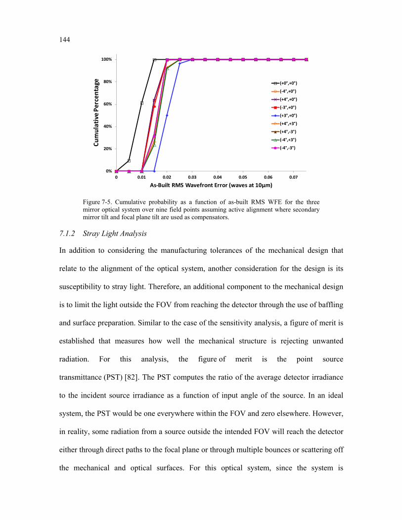
144
0%
20%
40%
60%
80%
100%
0 0.01 0.02 0.03 0.04 0.05 0.06 0.07
Cum
ulat
ive P
erce
ntag
e
As-Built RMS Wavefront Error (waves at 10µm)
(+0°,+0°)
(-4°,+0°)
(+4°,+0°)
(-3°,+0°)
(+3°,+0°)
(+4°,+3°)
(+4°,-3°)
(-4°,+3°)
(-4°,-3°)
Figure 7-5. Cumulative probability as a function of as-built RMS WFE for the three mirror optical system over nine field points assuming active alignment where secondary mirror tilt and focal plane tilt are used as compensators.
7.1.2 Stray Light Analysis
In addition to considering the manufacturing tolerances of the mechanical design that
relate to the alignment of the optical system, another consideration for the design is its
susceptibility to stray light. Therefore, an additional component to the mechanical design
is to limit the light outside the FOV from reaching the detector through the use of baffling
and surface preparation. Similar to the case of the sensitivity analysis, a figure of merit is
established that measures how well the mechanical structure is rejecting unwanted
radiation. For this analysis, the figure of merit is the point source
transmittance (PST) [82]. The PST computes the ratio of the average detector irradiance
to the incident source irradiance as a function of input angle of the source. In an ideal
system, the PST would be one everywhere within the FOV and zero elsewhere. However,
in reality, some radiation from a source outside the intended FOV will reach the detector
either through direct paths to the focal plane or through multiple bounces or scattering off
the mechanical and optical surfaces. For this optical system, since the system is
145
nonsymmetric, the PST will also be nonsymmetric. Furthermore, the optical system is
tilted only in the XZ plane so the primary contributor to the PST is the elevation angle of
the source. Using FRED, a non-sequential raytrace program from Photon Engineering,
the elevation PST of the optical system and base mechanical design presented in
Figure 7-1 is computed. In the software, rays from a 501x501, 120 mm diameter, 10 µm
source at the input aperture are traced in 1° increments over a 180° elevation. At each
input angle, the PST is computed. Figure 7-6 shows the log(PST) as a function of input
elevation angle for the base optical system where the optical surfaces are assumed to be
perfect reflectors and the walls of the optical housing are assumed to be near specular
with 80% reflectivity, which is a good representation for the specular component of
machined aluminum in the LWIR [83]. In Figure 7-6, it can be seen that the stray light
rejection of the base optical system is poor. There is a large region of stray light from
roughly 20° to 45° that results from a direct path to the focal plane from the input
aperture. A similar region of stray light is observed from -45° to -20° as the light in this
region reaches the focal plane by reflecting off one of the input faces of housing thus
creating a mirror image of the region between 20° and 45. These problem regions should
be mitigated to improve the overall signal-to-noise ratio of the optical system, if possible.
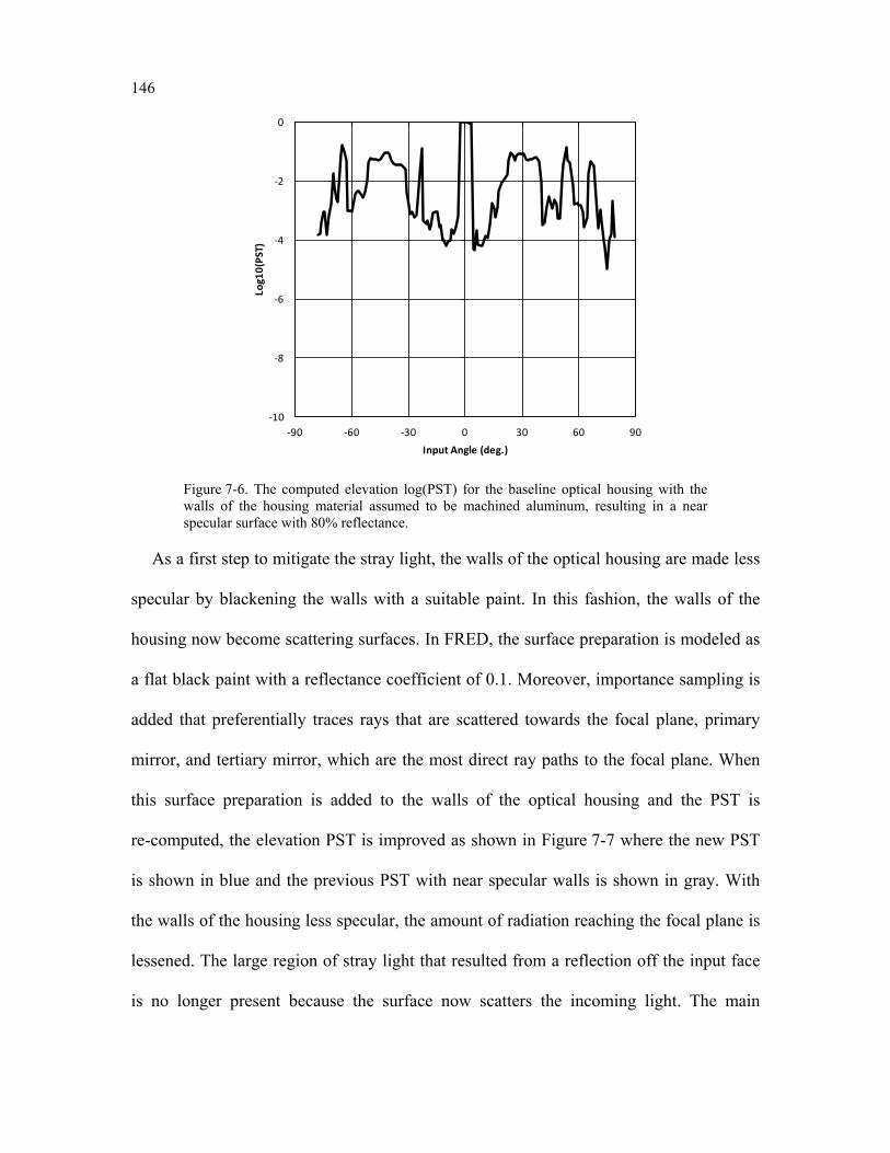
146
-10
-8
-6
-4
-2
0
-90 -60 -30 0 30 60 90
Log1
0(PS
T)
Input Angle (deg.)
Figure 7-6. The computed elevation log(PST) for the baseline optical housing with the walls of the housing material assumed to be machined aluminum, resulting in a near specular surface with 80% reflectance.
As a first step to mitigate the stray light, the walls of the optical housing are made less
specular by blackening the walls with a suitable paint. In this fashion, the walls of the
housing now become scattering surfaces. In FRED, the surface preparation is modeled as
a flat black paint with a reflectance coefficient of 0.1. Moreover, importance sampling is
added that preferentially traces rays that are scattered towards the focal plane, primary
mirror, and tertiary mirror, which are the most direct ray paths to the focal plane. When
this surface preparation is added to the walls of the optical housing and the PST is
re-computed, the elevation PST is improved as shown in Figure 7-7 where the new PST
is shown in blue and the previous PST with near specular walls is shown in gray. With
the walls of the housing less specular, the amount of radiation reaching the focal plane is
lessened. The large region of stray light that resulted from a reflection off the input face
is no longer present because the surface now scatters the incoming light. The main
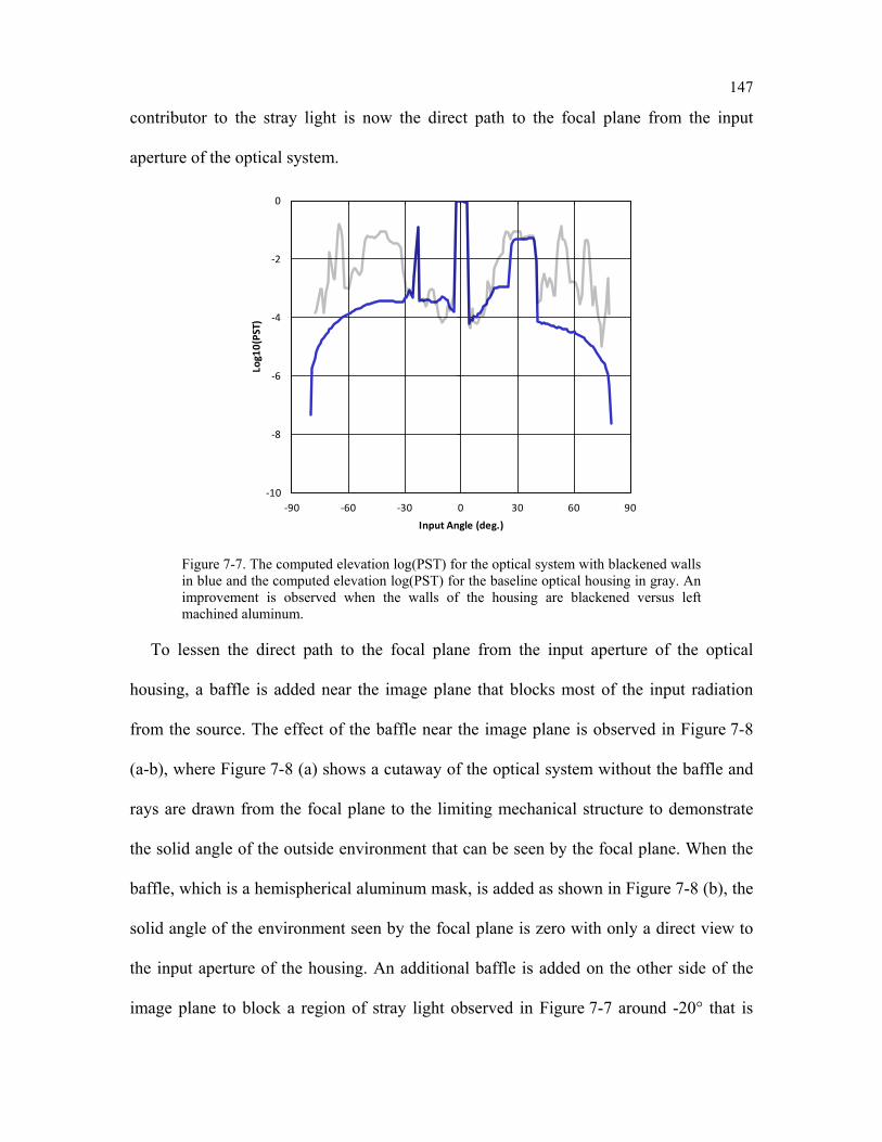
147
contributor to the stray light is now the direct path to the focal plane from the input
aperture of the optical system.
-10
-8
-6
-4
-2
0
-90 -60 -30 0 30 60 90
Log1
0(PS
T)
Input Angle (deg.)
Figure 7-7. The computed elevation log(PST) for the optical system with blackened walls in blue and the computed elevation log(PST) for the baseline optical housing in gray. An improvement is observed when the walls of the housing are blackened versus left machined aluminum.
To lessen the direct path to the focal plane from the input aperture of the optical
housing, a baffle is added near the image plane that blocks most of the input radiation
from the source. The effect of the baffle near the image plane is observed in Figure 7-8
(a-b), where Figure 7-8 (a) shows a cutaway of the optical system without the baffle and
rays are drawn from the focal plane to the limiting mechanical structure to demonstrate
the solid angle of the outside environment that can be seen by the focal plane. When the
baffle, which is a hemispherical aluminum mask, is added as shown in Figure 7-8 (b), the
solid angle of the environment seen by the focal plane is zero with only a direct view to
the input aperture of the housing. An additional baffle is added on the other side of the
image plane to block a region of stray light observed in Figure 7-7 around -20° that is
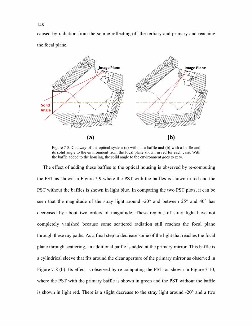
148
caused by radiation from the source reflecting off the tertiary and primary and reaching
the focal plane.
Image Plane Image Plane
(a) (b)
Solid Angle
Figure 7-8. Cutaway of the optical system (a) without a baffle and (b) with a baffle and its solid angle to the environment from the focal plane shown in red for each case. With the baffle added to the housing, the solid angle to the environment goes to zero.
The effect of adding these baffles to the optical housing is observed by re-computing
the PST as shown in Figure 7-9 where the PST with the baffles is shown in red and the
PST without the baffles is shown in light blue. In comparing the two PST plots, it can be
seen that the magnitude of the stray light around -20° and between 25° and 40° has
decreased by about two orders of magnitude. These regions of stray light have not
completely vanished because some scattered radiation still reaches the focal plane
through these ray paths. As a final step to decrease some of the light that reaches the focal
plane through scattering, an additional baffle is added at the primary mirror. This baffle is
a cylindrical sleeve that fits around the clear aperture of the primary mirror as observed in
Figure 7-8 (b). Its effect is observed by re-computing the PST, as shown in Figure 7-10,
where the PST with the primary baffle is shown in green and the PST without the baffle
is shown in light red. There is a slight decrease to the stray light around -20° and a two
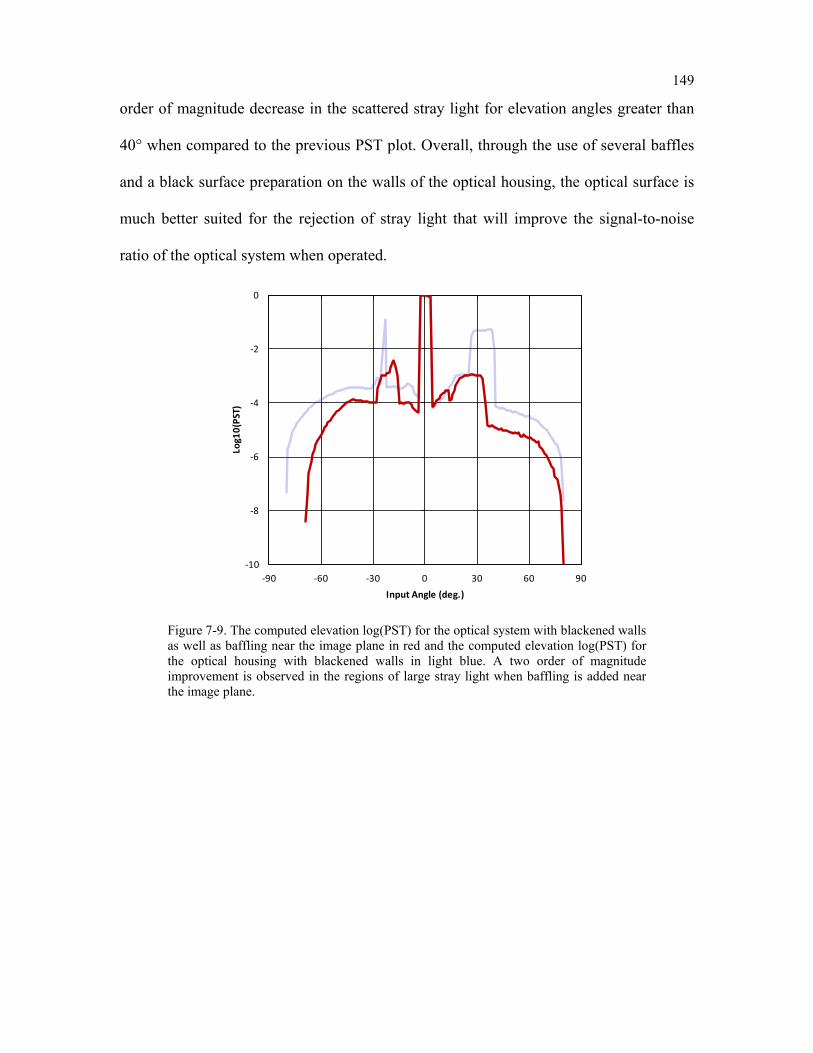
149
order of magnitude decrease in the scattered stray light for elevation angles greater than
40° when compared to the previous PST plot. Overall, through the use of several baffles
and a black surface preparation on the walls of the optical housing, the optical surface is
much better suited for the rejection of stray light that will improve the signal-to-noise
ratio of the optical system when operated.
-10
-8
-6
-4
-2
0
-90 -60 -30 0 30 60 90
Log1
0(PS
T)
Input Angle (deg.)
Figure 7-9. The computed elevation log(PST) for the optical system with blackened walls as well as baffling near the image plane in red and the computed elevation log(PST) for the optical housing with blackened walls in light blue. A two order of magnitude improvement is observed in the regions of large stray light when baffling is added near the image plane.
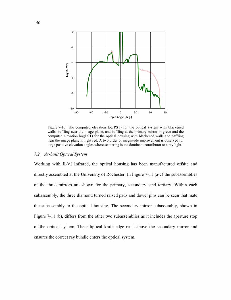
150
-10
-8
-6
-4
-2
0
-90 -60 -30 0 30 60 90
Log1
0(PS
T)
Input Angle (deg.)
Figure 7-10. The computed elevation log(PST) for the optical system with blackened walls, baffling near the image plane, and baffling at the primary mirror in green and the computed elevation log(PST) for the optical housing with blackened walls and baffling near the image plane in light red. A two order of magnitude improvement is observed for large positive elevation angles where scattering is the dominant contributor to stray light.
7.2 As-built Optical System
Working with II-VI Infrared, the optical housing has been manufactured offsite and
directly assembled at the University of Rochester. In Figure 7-11 (a-c) the subassemblies
of the three mirrors are shown for the primary, secondary, and tertiary. Within each
subassembly, the three diamond turned raised pads and dowel pins can be seen that mate
the subassembly to the optical housing. The secondary mirror subassembly, shown in
Figure 7-11 (b), differs from the other two subassemblies as it includes the aperture stop
of the optical system. The elliptical knife edge rests above the secondary mirror and
ensures the correct ray bundle enters the optical system.
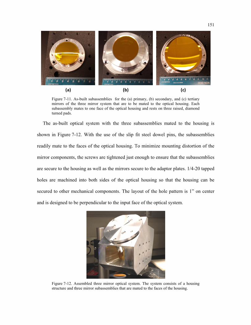
151
(a) (b) (c)
Figure 7-11. As-built subassemblies for the (a) primary, (b) secondary, and (c) tertiary mirrors of the three mirror system that are to be mated to the optical housing. Each subassembly mates to one face of the optical housing and rests on three raised, diamond turned pads.
The as-built optical system with the three subassemblies mated to the housing is
shown in Figure 7-12. With the use of the slip fit steel dowel pins, the subassemblies
readily mate to the faces of the optical housing. To minimize mounting distortion of the
mirror components, the screws are tightened just enough to ensure that the subassemblies
are secure to the housing as well as the mirrors secure to the adaptor plates. 1/4-20 tapped
holes are machined into both sides of the optical housing so that the housing can be
secured to other mechanical components. The layout of the hole pattern is 1” on center
and is designed to be perpendicular to the input face of the optical system.
Figure 7-12. Assembled three mirror optical system. The system consists of a housing structure and three mirror subassemblies that are mated to the faces of the housing.
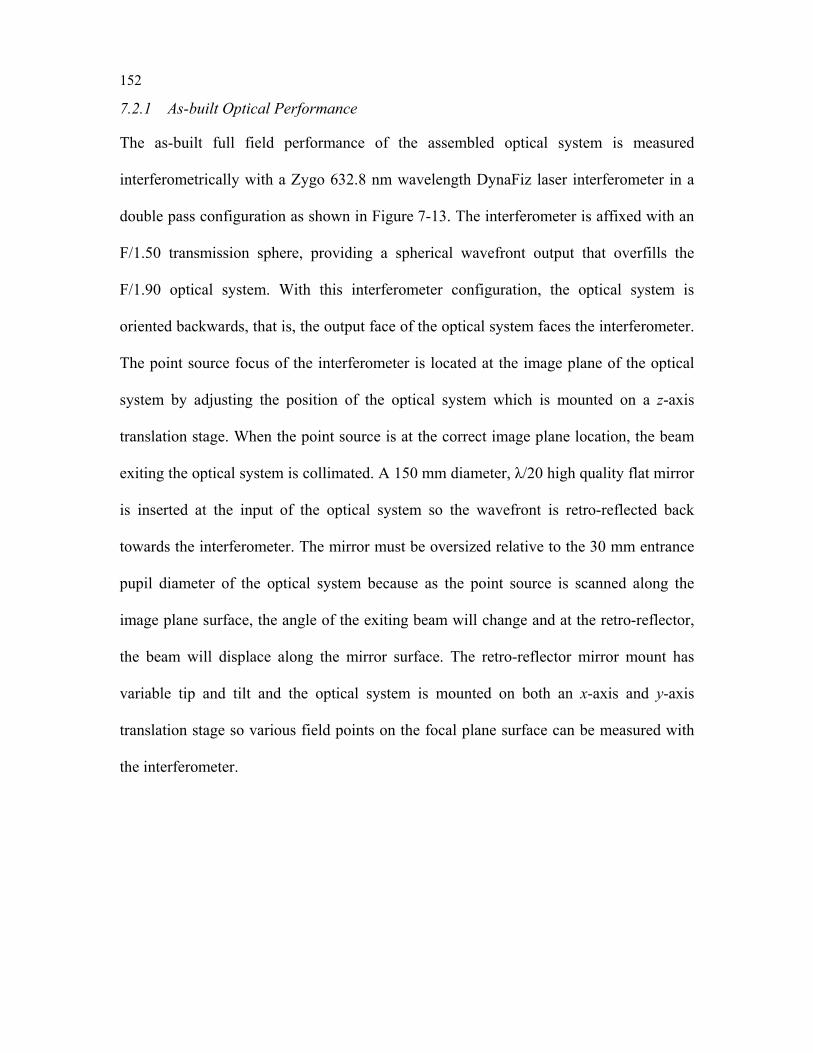
152
7.2.1 As-built Optical Performance
The as-built full field performance of the assembled optical system is measured
interferometrically with a Zygo 632.8 nm wavelength DynaFiz laser interferometer in a
double pass configuration as shown in Figure 7-13. The interferometer is affixed with an
F/1.50 transmission sphere, providing a spherical wavefront output that overfills the
F/1.90 optical system. With this interferometer configuration, the optical system is
oriented backwards, that is, the output face of the optical system faces the interferometer.
The point source focus of the interferometer is located at the image plane of the optical
system by adjusting the position of the optical system which is mounted on a z-axis
translation stage. When the point source is at the correct image plane location, the beam
exiting the optical system is collimated. A 150 mm diameter, λ/20 high quality flat mirror
is inserted at the input of the optical system so the wavefront is retro-reflected back
towards the interferometer. The mirror must be oversized relative to the 30 mm entrance
pupil diameter of the optical system because as the point source is scanned along the
image plane surface, the angle of the exiting beam will change and at the retro-reflector,
the beam will displace along the mirror surface. The retro-reflector mirror mount has
variable tip and tilt and the optical system is mounted on both an x-axis and y-axis
translation stage so various field points on the focal plane surface can be measured with
the interferometer.
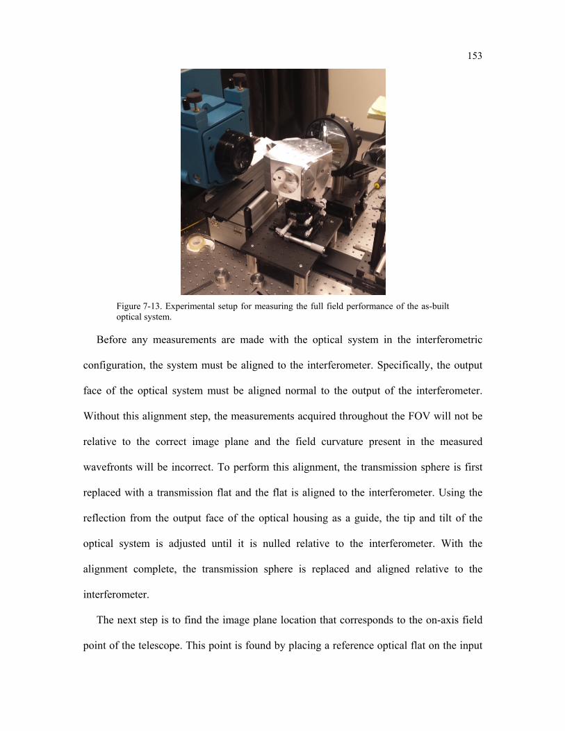
153
Figure 7-13. Experimental setup for measuring the full field performance of the as-built optical system.
Before any measurements are made with the optical system in the interferometric
configuration, the system must be aligned to the interferometer. Specifically, the output
face of the optical system must be aligned normal to the output of the interferometer.
Without this alignment step, the measurements acquired throughout the FOV will not be
relative to the correct image plane and the field curvature present in the measured
wavefronts will be incorrect. To perform this alignment, the transmission sphere is first
replaced with a transmission flat and the flat is aligned to the interferometer. Using the
reflection from the output face of the optical housing as a guide, the tip and tilt of the
optical system is adjusted until it is nulled relative to the interferometer. With the
alignment complete, the transmission sphere is replaced and aligned relative to the
interferometer.
The next step is to find the image plane location that corresponds to the on-axis field
point of the telescope. This point is found by placing a reference optical flat on the input
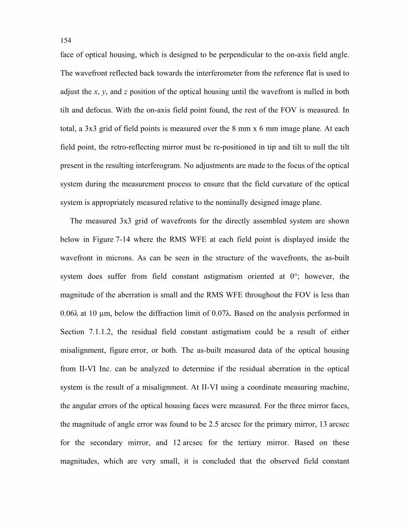
154
face of optical housing, which is designed to be perpendicular to the on-axis field angle.
The wavefront reflected back towards the interferometer from the reference flat is used to
adjust the x, y, and z position of the optical housing until the wavefront is nulled in both
tilt and defocus. With the on-axis field point found, the rest of the FOV is measured. In
total, a 3x3 grid of field points is measured over the 8 mm x 6 mm image plane. At each
field point, the retro-reflecting mirror must be re-positioned in tip and tilt to null the tilt
present in the resulting interferogram. No adjustments are made to the focus of the optical
system during the measurement process to ensure that the field curvature of the optical
system is appropriately measured relative to the nominally designed image plane.
The measured 3x3 grid of wavefronts for the directly assembled system are shown
below in Figure 7-14 where the RMS WFE at each field point is displayed inside the
wavefront in microns. As can be seen in the structure of the wavefronts, the as-built
system does suffer from field constant astigmatism oriented at 0°; however, the
magnitude of the aberration is small and the RMS WFE throughout the FOV is less than
0.06λ at 10 µm, below the diffraction limit of 0.07λ. Based on the analysis performed in
Section 7.1.1.2, the residual field constant astigmatism could be a result of either
misalignment, figure error, or both. The as-built measured data of the optical housing
from II-VI Inc. can be analyzed to determine if the residual aberration in the optical
system is the result of a misalignment. At II-VI using a coordinate measuring machine,
the angular errors of the optical housing faces were measured. For the three mirror faces,
the magnitude of angle error was found to be 2.5 arcsec for the primary mirror, 13 arcsec
for the secondary mirror, and 12 arcsec for the tertiary mirror. Based on these
magnitudes, which are very small, it is concluded that the observed field constant
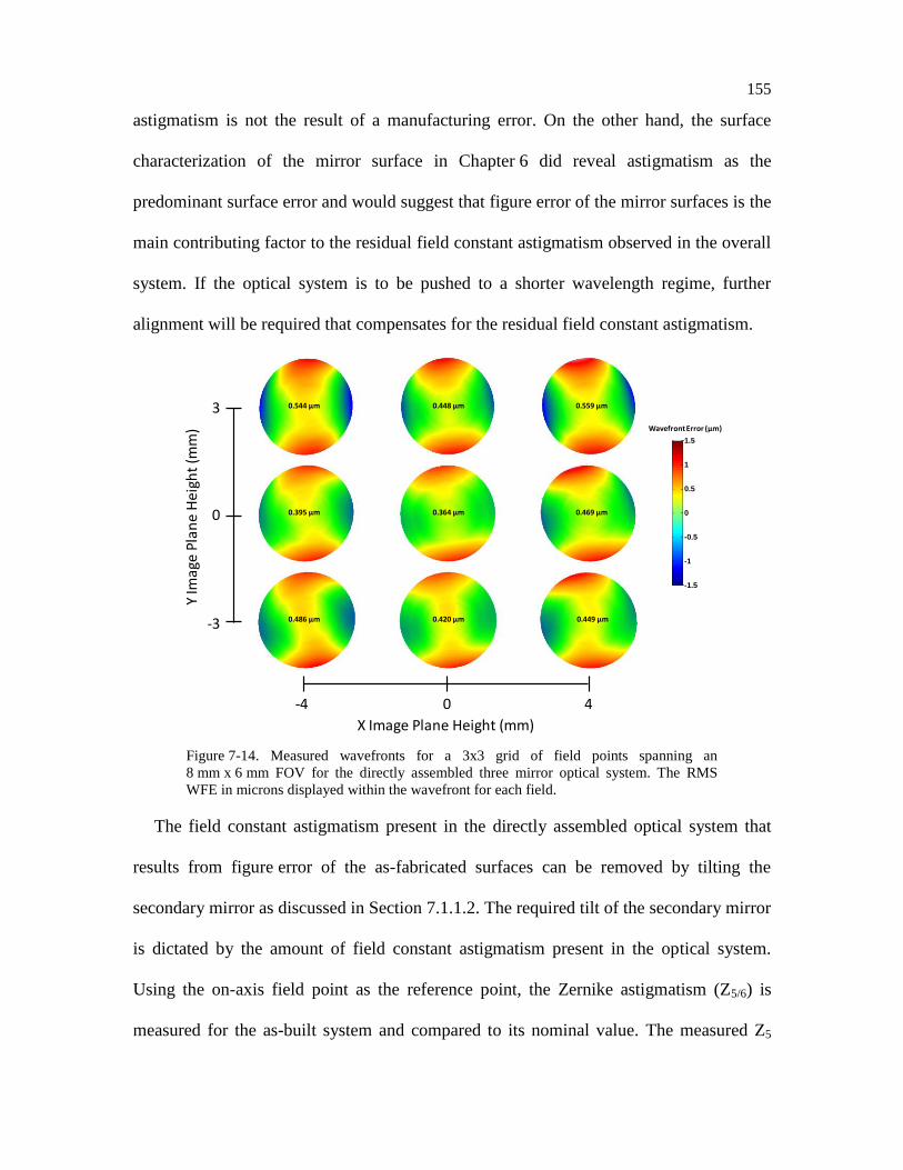
155
astigmatism is not the result of a manufacturing error. On the other hand, the surface
characterization of the mirror surface in Chapter 6 did reveal astigmatism as the
predominant surface error and would suggest that figure error of the mirror surfaces is the
main contributing factor to the residual field constant astigmatism observed in the overall
system. If the optical system is to be pushed to a shorter wavelength regime, further
alignment will be required that compensates for the residual field constant astigmatism.
0 0.2 0.4 0.6 0.8 10
0.2
0.4
0.6
0.8
1
-1.5
-1
-0.5
0
0.5
1
1.5
0.364 µm
0.448 µm
0.420 µm
0.544 µm
0.395 µm
0.486 µm 0.449 µm
0.469 µm
0.559 µm
Wavefront Error (µm)
0 4-4
0
3
-3
X Image Plane Height (mm)
Y Im
age
Pla
ne
He
igh
t (m
m)
Figure 7-14. Measured wavefronts for a 3x3 grid of field points spanning an
8 mm x 6 mm FOV for the directly assembled three mirror optical system. The RMS
WFE in microns displayed within the wavefront for each field.
The field constant astigmatism present in the directly assembled optical system that
results from figure error of the as-fabricated surfaces can be removed by tilting the
secondary mirror as discussed in Section 7.1.1.2. The required tilt of the secondary mirror
is dictated by the amount of field constant astigmatism present in the optical system.
Using the on-axis field point as the reference point, the Zernike astigmatism (Z5/6) is
measured for the as-built system and compared to its nominal value. The measured Z5
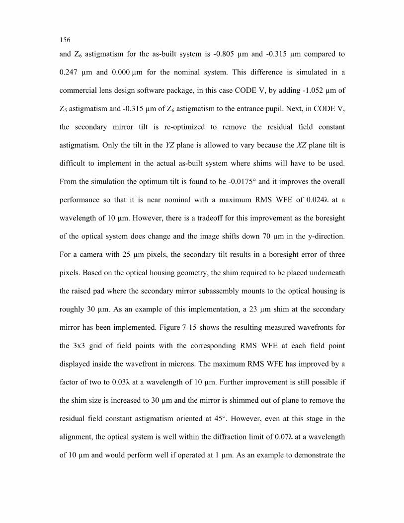
156
and Z6 astigmatism for the as-built system is -0.805 µm and -0.315 µm compared to
0.247 µm and 0.000 µm for the nominal system. This difference is simulated in a
commercial lens design software package, in this case CODE V, by adding -1.052 µm of
Z5 astigmatism and -0.315 µm of Z6 astigmatism to the entrance pupil. Next, in CODE V,
the secondary mirror tilt is re-optimized to remove the residual field constant
astigmatism. Only the tilt in the YZ plane is allowed to vary because the XZ plane tilt is
difficult to implement in the actual as-built system where shims will have to be used.
From the simulation the optimum tilt is found to be -0.0175° and it improves the overall
performance so that it is near nominal with a maximum RMS WFE of 0.024λ at a
wavelength of 10 µm. However, there is a tradeoff for this improvement as the boresight
of the optical system does change and the image shifts down 70 µm in the y-direction.
For a camera with 25 µm pixels, the secondary tilt results in a boresight error of three
pixels. Based on the optical housing geometry, the shim required to be placed underneath
the raised pad where the secondary mirror subassembly mounts to the optical housing is
roughly 30 µm. As an example of this implementation, a 23 µm shim at the secondary
mirror has been implemented. Figure 7-15 shows the resulting measured wavefronts for
the 3x3 grid of field points with the corresponding RMS WFE at each field point
displayed inside the wavefront in microns. The maximum RMS WFE has improved by a
factor of two to 0.03λ at a wavelength of 10 µm. Further improvement is still possible if
the shim size is increased to 30 µm and the mirror is shimmed out of plane to remove the
residual field constant astigmatism oriented at 45°. However, even at this stage in the
alignment, the optical system is well within the diffraction limit of 0.07λ at a wavelength
of 10 µm and would perform well if operated at 1 µm. As an example to demonstrate the
157
image quality of the assembled optical system, Figure 7-16 shows a sample image of the
optical system affixed with the 8 mm x 6 mm, 25 µm pixel pitch uncooled
microbolometer detector.
0 0.2 0.4 0.6 0.8 10
0.2
0.4
0.6
0.8
1
-1
-0.5
0
0.5
1
0.157 µm
0.213 µm
0.192 µm
0.297 µm
0.201 µm
0.298 µm 0.242 µm
0.208 µm
0.295 µm
Wavefront Error (µm)
0 4-4
0
3
-3
X Image Plane Height (mm)
Y Im
age
Pla
ne
He
igh
t (m
m)
Figure 7-15. Measured wavefronts for a 3x3 grid of field points spanning an
8 mm x 6 mm FOV for the directly assembled three mirror optical system with the
secondary mirror tilted roughly 1 arc minute with a 23 µm shim. The RMS WFE in
microns is displayed within the wavefront for each field.
Figure 7-16. Sample LWIR image from the optical system
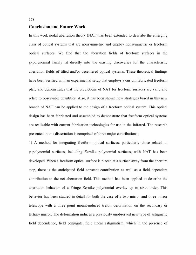
158
Conclusion and Future Work
In this work nodal aberration theory (NAT) has been extended to describe the emerging
class of optical systems that are nonsymmetric and employ nonsymmetric or freeform
optical surfaces. We find that the aberration fields of freeform surfaces in the
ϕ-polynomial family fit directly into the existing discoveries for the characteristic
aberration fields of tilted and/or decentered optical systems. These theoretical findings
have been verified with an experimental setup that employs a custom fabricated freeform
plate and demonstrates that the predictions of NAT for freeform surfaces are valid and
relate to observable quantities. Also, it has been shown how strategies based in this new
branch of NAT can be applied to the design of a freeform optical system. This optical
design has been fabricated and assembled to demonstrate that freeform optical systems
are realizable with current fabrication technologies for use in the infrared. The research
presented in this dissertation is comprised of three major contributions:
1) A method for integrating freeform optical surfaces, particularly those related to
ϕ-polynomial surfaces, including Zernike polynomial surfaces, with NAT has been
developed. When a freeform optical surface is placed at a surface away from the aperture
stop, there is the anticipated field constant contribution as well as a field dependent
contribution to the net aberration field. This method has been applied to describe the
aberration behavior of a Fringe Zernike polynomial overlay up to sixth order. This
behavior has been studied in detail for both the case of a two mirror and three mirror
telescope with a three point mount-induced trefoil deformation on the secondary or
tertiary mirror. The deformation induces a previously unobserved new type of astigmatic
field dependence, field conjugate, field linear astigmatism, which in the presence of
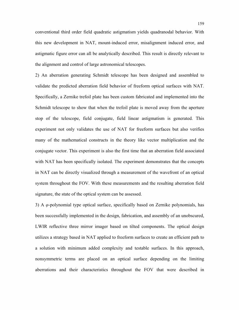
159
conventional third order field quadratic astigmatism yields quadranodal behavior. With
this new development in NAT, mount-induced error, misalignment induced error, and
astigmatic figure error can all be analytically described. This result is directly relevant to
the alignment and control of large astronomical telescopes.
2) An aberration generating Schmidt telescope has been designed and assembled to
validate the predicted aberration field behavior of freeform optical surfaces with NAT.
Specifically, a Zernike trefoil plate has been custom fabricated and implemented into the
Schmidt telescope to show that when the trefoil plate is moved away from the aperture
stop of the telescope, field conjugate, field linear astigmatism is generated. This
experiment not only validates the use of NAT for freeform surfaces but also verifies
many of the mathematical constructs in the theory like vector multiplication and the
conjugate vector. This experiment is also the first time that an aberration field associated
with NAT has been specifically isolated. The experiment demonstrates that the concepts
in NAT can be directly visualized through a measurement of the wavefront of an optical
system throughout the FOV. With these measurements and the resulting aberration field
signature, the state of the optical system can be assessed.
3) A φ-polynomial type optical surface, specifically based on Zernike polynomials, has
been successfully implemented in the design, fabrication, and assembly of an unobscured,
LWIR reflective three mirror imager based on tilted components. The optical design
utilizes a strategy based in NAT applied to freeform surfaces to create an efficient path to
a solution with minimum added complexity and testable surfaces. In this approach,
nonsymmetric terms are placed on an optical surface depending on the limiting
aberrations and their characteristics throughout the FOV that were described in
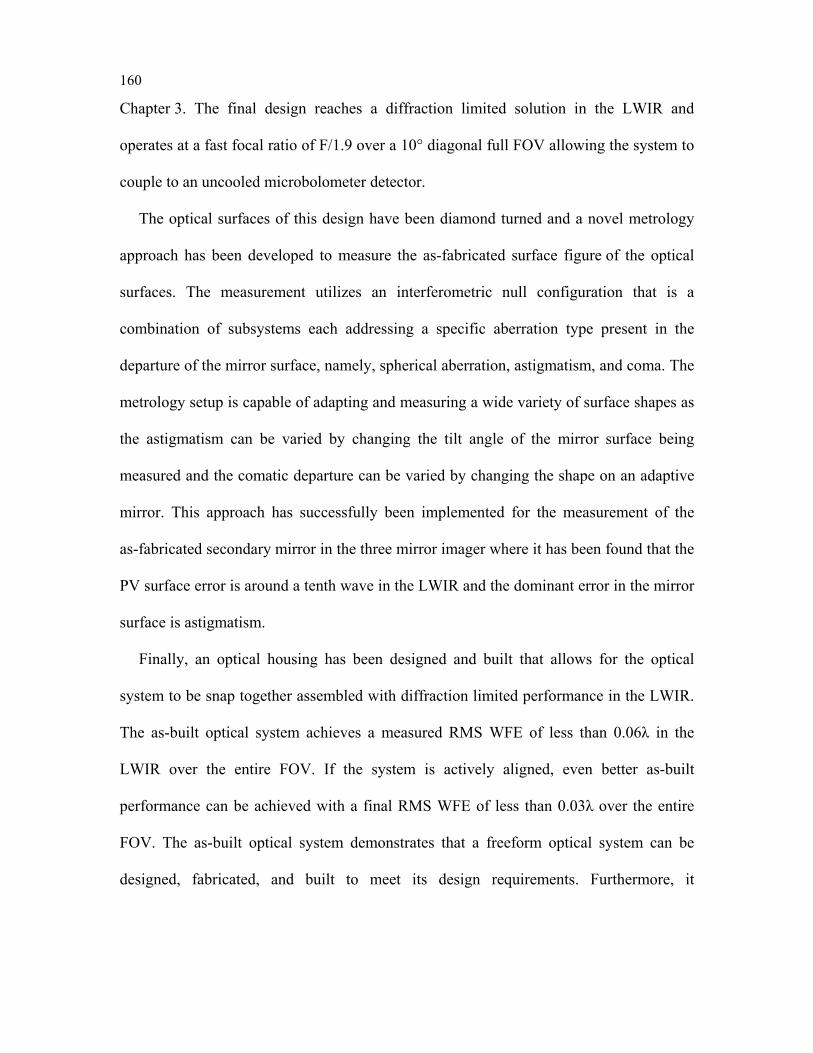
160
Chapter 3. The final design reaches a diffraction limited solution in the LWIR and
operates at a fast focal ratio of F/1.9 over a 10° diagonal full FOV allowing the system to
couple to an uncooled microbolometer detector.
The optical surfaces of this design have been diamond turned and a novel metrology
approach has been developed to measure the as-fabricated surface figure of the optical
surfaces. The measurement utilizes an interferometric null configuration that is a
combination of subsystems each addressing a specific aberration type present in the
departure of the mirror surface, namely, spherical aberration, astigmatism, and coma. The
metrology setup is capable of adapting and measuring a wide variety of surface shapes as
the astigmatism can be varied by changing the tilt angle of the mirror surface being
measured and the comatic departure can be varied by changing the shape on an adaptive
mirror. This approach has successfully been implemented for the measurement of the
as-fabricated secondary mirror in the three mirror imager where it has been found that the
PV surface error is around a tenth wave in the LWIR and the dominant error in the mirror
surface is astigmatism.
Finally, an optical housing has been designed and built that allows for the optical
system to be snap together assembled with diffraction limited performance in the LWIR.
The as-built optical system achieves a measured RMS WFE of less than 0.06λ in the
LWIR over the entire FOV. If the system is actively aligned, even better as-built
performance can be achieved with a final RMS WFE of less than 0.03λ over the entire
FOV. The as-built optical system demonstrates that a freeform optical system can be
designed, fabricated, and built to meet its design requirements. Furthermore, it
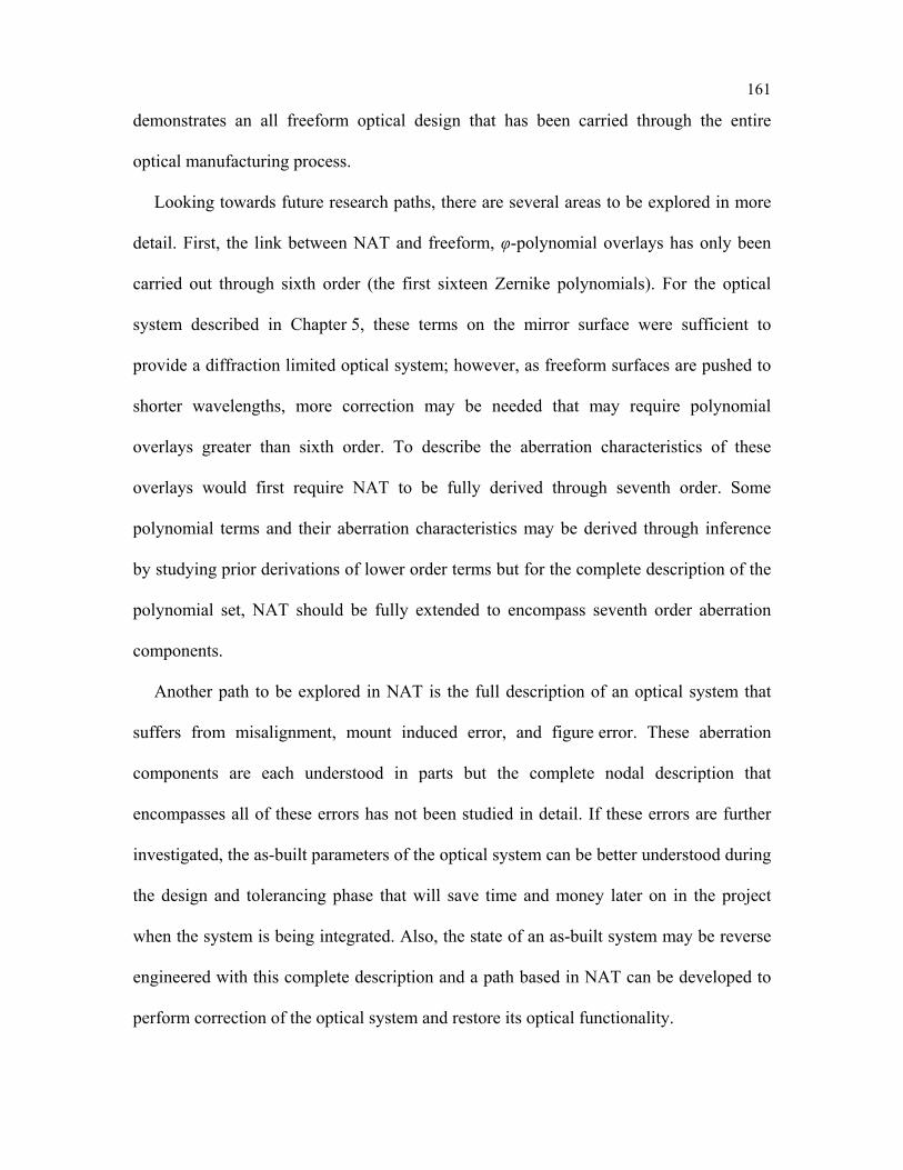
161
demonstrates an all freeform optical design that has been carried through the entire
optical manufacturing process.
Looking towards future research paths, there are several areas to be explored in more
detail. First, the link between NAT and freeform, φ-polynomial overlays has only been
carried out through sixth order (the first sixteen Zernike polynomials). For the optical
system described in Chapter 5, these terms on the mirror surface were sufficient to
provide a diffraction limited optical system; however, as freeform surfaces are pushed to
shorter wavelengths, more correction may be needed that may require polynomial
overlays greater than sixth order. To describe the aberration characteristics of these
overlays would first require NAT to be fully derived through seventh order. Some
polynomial terms and their aberration characteristics may be derived through inference
by studying prior derivations of lower order terms but for the complete description of the
polynomial set, NAT should be fully extended to encompass seventh order aberration
components.
Another path to be explored in NAT is the full description of an optical system that
suffers from misalignment, mount induced error, and figure error. These aberration
components are each understood in parts but the complete nodal description that
encompasses all of these errors has not been studied in detail. If these errors are further
investigated, the as-built parameters of the optical system can be better understood during
the design and tolerancing phase that will save time and money later on in the project
when the system is being integrated. Also, the state of an as-built system may be reverse
engineered with this complete description and a path based in NAT can be developed to
perform correction of the optical system and restore its optical functionality.
162
Beyond NAT, an interesting aspect of this work has been the fabrication and
metrology of freeform surfaces. A flexible approach has been presented that utilizes an
active or deformable membrane mirror surface. While the DM is able to create a wide
variety of shapes, it suffers large surface errors resulting from local deformations at the
actuator sites. Based on the success of fabricating freeform components with sub-aperture
polishing processes like MRF (see Chapter 4), one area to be explored is to fabricate
using MRF the comatic null shape that has historically been placed on the active mirror.
With this implementation, the need for a software null to remove the residual error
present from the active mirror in the final measurement may be eliminated.
Lastly, in this dissertation, only one example of freeform optical surfaces for
unobscured reflective design has been presented. An interesting exercise would be to
explore the design space further where the tools developed in this dissertation are utilized
to guide the addition of freeform overlay terms on the optical surfaces. Also, it would be
useful to find solutions for shorter wavelength regimes where the focal ratio does not
need to be as fast. Based on the work presented in this dissertation, the fabrication
capabilities exist to assemble an optical system for the short wave infrared with near
diffraction limited performance.
163
Appendix A. Vector Multiplication and Its Vector Properties and Identities
Nodal aberration theory makes use of a vector operation known as vector multiplication.
The resultant is a coplanar vector and the operation requires the use of an absolute
coordinate system. In this appendix, vector multiplication is introduced and some of its
properties and identities are summarized following the work of Thompson [20, 59].
Vector Multiplication
When describing the concepts of vector multiplication, the analogy of multiplying two
complex numbers is often used. Consider two vectors A
and B
that are expressed as
ˆ ˆ,ix yA ae a i a jα= = +
(A.1)
and
ˆ ˆ,ix yB be b i b jβ= = +
(A.2)
where
sin , cos ,
sin , cos ,x y
x y
a a a ab b b b
α α
β β
= =
= = (A.3)
and the coordinate system in Figure A-1 is used. Multiplying these vectors gives
( ) ( )( ) ˆ ˆ.iy x x y y y x xAB abe a b a b i a b a b jα β+= = + + −
(A.4)
The resultant AB
is a vector with a magnitude equal to the product of the magnitudes of
vectors A
and B
and an orientation that is the sum of the orientations of vectors A
and B
.
The operation is further illustrated in Figure A-1.
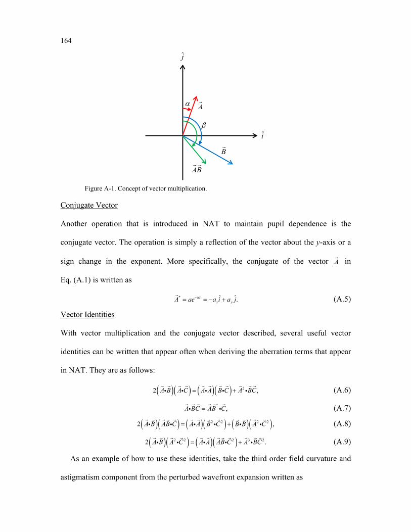
164
A
B
AB
α
βi
j
Figure A-1. Concept of vector multiplication.
Conjugate Vector
Another operation that is introduced in NAT to maintain pupil dependence is the
conjugate vector. The operation is simply a reflection of the vector about the y-axis or a
sign change in the exponent. More specifically, the conjugate of the vector A
in
Eq. (A.1) is written as
* ˆ ˆ.ix yA ae a i a jα−= = − +
(A.5)
Vector Identities
With vector multiplication and the conjugate vector described, several useful vector
identities can be written that appear often when deriving the aberration terms that appear
in NAT. They are as follows:
( )( ) ( )( ) 22 ,A B A C A A B C A BC= +
(A.6)
*
,A BC AB C=
(A.7)
( )( ) ( )( ) ( )( )2 2 2 22 ,A B AB C A A B C B B A C= +
(A.8)
( )( ) ( )( )2 2 2 3 22 .A B A C A A AB C A BC= +
(A.9)
As an example of how to use these identities, take the third order field curvature and
astigmatism component from the perturbed wavefront expansion written as
165
( ) ( ) ( ) ( ).2
220 222 .j jS j j j
j jW W H H W Hσ σ ρ ρ σ ρ = − − + − ∑ ∑
(A.10)
Now, using Eq. (A.6) where ( )A H σ= −
and B C ρ= =
, the third order astigmatism component
is re-written so that the wavefront takes the following form
( ) ( ) ( ) ( ) ( ) ( )
( )
220 222
2 2222
12
1 .2
j j
j
S j j j jj j
jj
W W H H W H H
W H
σ σ ρ ρ σ σ ρ ρ
σ ρ
= − − + − −
+ −
∑ ∑
∑
(A.11)
The first two terms in Eq. (A.11) relate to the medial focal surface that is defined as
220 220 2221 ,2M SW W W= + (A.12)
so that the wavefront expansion is re-written as
( ) ( ) ( ) ( )2 2220 222
1 .2j jM j j j
j jW W H H W Hσ σ ρ ρ σ ρ = − − + − ∑ ∑
(A.13)
166
List of References
1. D. Korsch, "Closed Form Solution for Three-Mirror Telescopes, Corrected for Spherical Aberration, Coma, Astigmatism, and Field Curvature," Appl. Opt. 11, 2986-2987 (1972).
2. D. Korsch, "Closed-form solutions for imaging systems, corrected for third-order aberrations," J. Opt. Soc. Am. 63, 667-672 (1973).
3. A. Rakich and N. Rumsey, "Method for deriving the complete solution set for three-mirror anastigmatic telescopes with two spherical mirrors," Journal of the Optical Society of America A 19, 1398-1405 (2002).
4. J. W. Figoski, "Aberration characteristics of nonsymmetric systems," Proc. SPIE 554, 104-111 (1985).
5. R. A. Buchroeder, "Tilted-Component Telescopes. Part I: Theory," Appl. Opt. 9, 2169-2171 (1970).
6. K. Fuerschbach, J. P. Rolland, and K. P. Thompson, "A new family of optical systems employing phi-polynomial surfaces," Opt. Express 19, 21919-21928 (2011).
7. L. G. Cook, "Three-mirror anastigmat used off-axis in aperture and field," Proc. SPIE 183, 207-211 (1979).
8. L. G. Cook, "Three mirror anastigmatic optical system," 4,265,510 (1981). 9. D. E. Korsch, "Anastigmatic Three-Mirror Telescope," 4101195 (1978). 10. I. R. Abel and M. R. Hatch, "The pursuit of symmetry in wide-angle reflective
optical designs," Proc. SPIE 237, 271-280 (1980). 11. J. G. Baker, "On Improving the Effectiveness of Large Telescopes," Aerospace and
Electronic Systems, IEEE Transactions AES-5, 261-272 (1969). 12. W. B. Wetherell and D. A. Womble, "All-reflective three element objective,"
4,240,707 (1980). 13. K. L. Hallam, B. J. Howell, and M. E. Wilson, "Wide-angle flat field telescope,"
4,598,981 (1986). 14. H. P. Brueggemann, Conic Mirrors (Focal Press, London, 1968). 15. I. M. Egdall, "Manufacture of a three-mirror wide-field optical system," Optical
Engineering 24, 285-289 (1985). 16. T. E. Jewell, J. M. Rodgers, and K. P. Thompson, "Reflective systems design study
for soft x-ray projection lithography," Journal of Vacuum Science & Technology B: Microelectronics and Nanometer Structures 8, 1519-1523 (1990).
17. A. Kutter, "The Schiefspiegler ( Oblique Telescope )," Sky and Telescope Bulletin A (1958).
18. R. A. Buchroeder and A. S. Leonard, "Wide-Field Tilted-Component Telescope: a Leonard Extended Yolo All-Reflecting System," Appl. Opt. 11, 1649-1651 (1972).
19. R. V. Shack and K. P. Thompson, "Influence of alignment errors of a telescope system," Proc. SPIE 251, 146-153 (1980).
20. K. Thompson, "Description of the third-order optical aberrations of near-circular pupil optical systems without symmetry," J. Opt. Soc. Am. A 22, 1389-1401 (2005).
21. K. P. Thompson, T. Schmid, and J. P. Rolland, "The misalignment induced aberrations of TMA telescopes," Opt. Express 16, 20345-20353 (2008).
167
22. K. P. Thompson, T. Schmid, O. Cakmakci, and J. P. Rolland, "Real-ray-based method for locating individual surface aberration field centers in imaging optical systems without rotational symmetry," J. Opt. Soc. Am. A 26, 1503-1517 (2009).
23. K. P. Thompson, "Multinodal fifth-order optical aberrations of optical systems without rotational symmetry: the comatic aberrations," J. Opt. Soc. Am. A 27, 1490-1504 (2010).
24. K. P. Thompson, "Multinodal fifth-order optical aberrations of optical systems without rotational symmetry: spherical aberration," J. Opt. Soc. Am. A 26, 1090-1100 (2009).
25. K. P. Thompson, "Multinodal fifth-order optical aberrations of optical systems without rotational symmetry: the astigmatic aberrations," J. Opt. Soc. Am. A 28, 821-836 (2011).
26. J. R. Rogers, "Vector aberration theory and the design of off-axis systems," Proc. SPIE 554, 76-81 (1985).
27. J. R. Rogers and S. Tachihara, "Practical Tilted Mirror Systems," Proc. SPIE 679, 12-16 (1986).
28. J. R. Rogers, "Techniques and tools for obtaining symmetrical performance from tilted-component systems," Optical Engineering 39, 1776-1787 (2000).
29. J. M. Howard and B. D. Stone, "Imaging with Three Spherical Mirrors," Appl. Opt. 39, 3216-3231 (2000).
30. T. Nakano and Y. Tamagawa, "Configuration of an off-axis three-mirror system focused on compactness and brightness," Appl. Opt. 44, 776-783 (2005).
31. W. T. Plummer, "Unusual optics of the Polaroid SX-70 Land camera," Applied Optics 21, 196-208 (1982).
32. B. Tatian, "Nonrotationally Symmetric Systems: A New Problem For Optical Design And Fabrication," Proc. SPIE 0039, 205-222 (1974).
33. B. Tatian, "Testing an unusual optical surface," Proc. SPIE 554, 139-147 (1985). 34. B. Tatian, "A First Look At The Computer Design Of Optical Systems Without Any
Symmetry," Proc. SPIE 766, 38-47 (1987). 35. R. W. Gray, C. Dunn, K. P. Thompson, and J. P. Rolland, "An analytic expression
for the field dependence of Zernike polynomials in rotationally symmetric optical systems," Opt. Express 20, 16436-16449 (2012).
36. G. W. Forbes, "Characterizing the shape of freeform optics," Optics Express 20, 2483-2499 (2012).
37. T. P. Vogl, A. K. Rigler, and B. R. Canty, "Asymmetric Lens Design Using Bicubic Splines: Application to the Color TV Lighthouse," Applied Optics 10, 2513-2516 (1971).
38. J. E. Stacy, "Asymmetric spline surfaces: characteristics and applications," Applied Optics 23, 2710-2714 (1984).
39. O. Cakmakci, B. Moore, H. Foroosh, and J. P. Rolland, "Optimal local shape description for rotationally non-symmetric optical surface design and analysis," Opt. Express 16, 1583-1589 (2008).
40. A. M. Bauer, K. P. Thompson, and J. P. Rolland, "Moving from φ-Polynomial to Multicentric Radial Basis Functions," in Freeform Optics Incubator (OSA, 2011),
41. I. Kaya and P. Rolland Jannick, "Hybrid RBF and local phi-polynomial freeform surfaces," in Advanced Optical Technologies, (2013), p. 81.
168
42. R. Gelles, "Unobscured-aperture two-mirror systems," J. Opt. Soc. Am. 65, 1141-1143 (1975).
43. D. Luttrell, "Machining non-axisymmetric optics," in 1990), 44. Y. E. Tohme and J. A. Lowe, "Machining of freeform optical surfaces by slow slide
servo method," in Proceedings of the American Society for Precision Engineering Annual Meeting, Proc. of the ASPE Annual Meeting 2004),
45. J. Schaefer, "Single Point Diamond Turning: Progress in Precision," in Technical Digest (CD) (Optical Society of America, 2006), ThB1.
46. R. Henselmans, N. Rosielle, M. Steinbuch, I. Saunders, and R. Bergmans, "Design of a machine for the universal non-contact measurement of large free-form optics with 30 nm uncertainty," in 2005), 586919-586919-586912.
47. S. DeFisher, E. Fess, and F. Wolfs, "Freeform and conformal optical manufacturing," in 2013), 870813-870813-870819.
48. J. C. Wyant and V. P. Bennett, "Using Computer Generated Holograms to Test Aspheric Wavefronts," Appl. Opt. 11, 2833-2839 (1972).
49. P. Zhou and J. H. Burge, "Fabrication error analysis and experimental demonstration for computer-generated holograms," Appl. Opt. 46, 657-663 (2007).
50. E. Savio, L. De Chiffre, and R. Schmitt, "Metrology of freeform shaped parts," CIRP Annals - Manufacturing Technology 56, 810-835 (2007).
51. M. C. Ruda, "Methods for null testing sections of aspheric surfaces," Ph.D. dissertation (University of Arizona, Optical Sciences Center, 1979).
52. D. Shafer, "Design with two-axis aspheric surfaces," in Computer-Aided Optical Design (SPIE, 1978), 171-176.
53. R. N. Wilson, Reflecting Telescope Optics I: Basic Design Theory and Its Historical Development (Springer, 2004), Vol. 1.
54. J. J. P. McGuire, "Manufacturable mobile phone optics: higher order aspheres are not always better," in 2010), 76521O-76521O-76528.
55. W. T. Welford, Aberrations of optical systems (CRC Press, 1986). 56. H. H. Hopkins, Wave theory of aberrations (Clarendon Press, 1950). 57. M. P. Rimmer, "Optical aberration coefficients," M.S. (University of Rochester,
Rocheser, NY, 1963). 58. J. M. Hoffman, "Induced Aberrations in Optical Systems," PhD (University of
Arizona, Tucson, AZ, 1993). 59. K. P. Thompson, "Aberration fields in tilted and decentered optical systems," Ph.D.
(The University of Arizona, 1980). 60. K. P. Thompson, "Beyond Optical Design: Interaction between the lens designer and
the real world," Proc. SPIE 554, 426-438 (1985). 61. "Zernike Polynomials," in CODE V Reference Manual (2012), pp. Volume IV,
Appendix C. 62. A. B. Bhatia and E. Wolf, "On the Circle Polynomials of Zernike and Related
Orthogonal Sets," Proc. Cambridge Philos. Soc. 50, 40-48 (1954). 63. C. J. Evans, "PVr—a robust amplitude parameter for optical surface specification,"
Optical Engineering 48, 043605-043605-043608 (2009). 64. T. Schmid, J. P. Rolland, A. Rakich, and K. P. Thompson, "Separation of the effects
of astigmatic figure error from misalignments using Nodal Aberration Theory (NAT)," Opt. Express 18, 17433-17447 (2010).
169
65. K. P. Thompson, "Aberration fields in unobscured mirror systems," J. Opt. Soc. Am. 103, 159-165 (1980).
66. J. Wang, B. Guo, Q. Sun, and Z. Lu, "Third-order aberration fields of pupil decentered optical systems," Opt. Express 20, 11652-11658 (2012).
67. K. P. Thompson, "Reinterpreting Coddington: correcting 150 years of confusion," in Robert Shannon and Roland Shack, Legends in Applied Optics, J. E. Harvey and R. B. Hooker, eds. (SPIE Press, 2005), pp. 41-49.
68. C. R. Burch, "On the optical see-saw diagram," Mon. Not. R. Astron. Soc. 103, 159-165 (1942).
69. A. Rakich, "Calculation of third-order misalignment aberrations with the optical plate diagram," Proc. SPIE 7652, 765230-765211 (2010).
70. K. Fuerschbach, J. P. Rolland, and K. P. Thompson, "Aberration behavior of a classical two-mirror telescope in the presence of mount error using nodal aberration theory," in OSA Technical Digest (online) (Optical Society of America, 2012), FTu5F.2.
71. J. E. Stacy and S. A. Macenka, "Optimization of an unobscured optical system using vector aberration theory," Proc. SPIE 679, 21-24 (1986).
72. K. B. Doyle, V. L. Genberg, and G. J. Michels, Integrated optomechanical analysis (SPIE press, 2002), Vol. 58.
73. J. Nella, P. D. Atcheson, C. B. Atkinson, D. Au, A. J. Bronowicki, E. Bujanda, A. Cohen, D. Davies, P. A. Lightsey, R. Lynch, R. Lundquist, M. T. Menzel, M. Mohan, J. Pohner, P. Reynolds, H. Rivera, S. C. Texter, D. V. Shuckstes, D. D. F. Simmons, R. C. Smith, P. C. Sullivan, D. D. Waldie, and R. Woods, "James Webb Space Telescope (JWST) Observatory architecture and performance," Proc. SPIE 5487, 576-587 (2004).
74. "Three Mirror Objective," Aerial Camera Lenses, 027000 (Air Force Avionics Laboratory, 1967).
75. J. M. Rodgers, "Catoptric optical system including concave and convex reflectors," 5,309,276 (1994).
76. A. Offner, "A Null Corrector for Paraboloidal Mirrors," Appl. Opt. 2, 153-155 (1963).
77. C. Pruss and H. J. Tiziani, "Dynamic null lens for aspheric testing using a membrane mirror," Optics Communications 233, 15-19 (2004).
78. H. Coddington, Coddinton, Henry; A Treatise on the Reflection and Refraction of Light, Part 1 (Cambridge, UK, 1829).
79. J. Schwiegerling, J. E. Greivenkamp, and J. M. Miller, "Representation of videokeratoscopic height data with Zernike polynomials," J. Opt. Soc. Am. A 12, 2105-2113 (1995).
80. T. Scheimpflug, "Improved Method and Apparatus for the Systematic Alteration or Distortion of Plane Pictures and Images by Means of Lenses and Mirrors for Photography and for other purposes," 1196 (May 12 1904).
81. J. H. Hindle, "A New Test for Cassegrainian and Gregorian Secondary Mirrors," Mon. Not. R. Astron. Soc. 91, 592 (1931).
82. R. P. Breault, "Control of Stray Light," in Handbook of optics, 3rd ed., M. Bass, ed. (McGraw-Hill, New York, 2009).

170
83. J. Bortle, "A Measurement- and Prediction-Based Validation of the AFIT Large Commercial Aircraft Infrared Trend Analysis Tool.," Masters' thesis (Air Force Institute of Technology (AETC), Wright-Patterson AFB, OH, 2006).