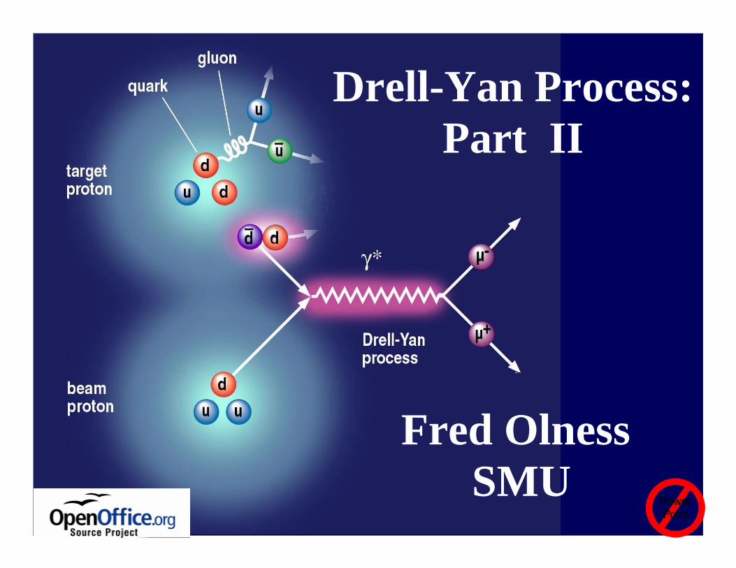
Drell-Yan Process:Part II

Fred Olness SMU

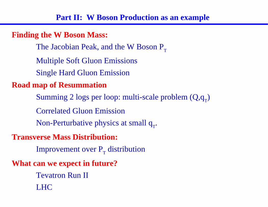
Part II: W Boson Production as an example

Finding the W Boson Mass:

The Jacobian Peak, and the W Boson PT

Multiple Soft Gluon Emissions

Single Hard Gluon Emission

Road map of Resummation

Summing 2 logs per loop: multi-scale problem (Q,qT)

Correlated Gluon Emission

Non-Perturbative physics at small qT.

Transverse Mass Distribution:

Improvement over PT distribution

What can we expect in future?

Tevatron Run II

LHC

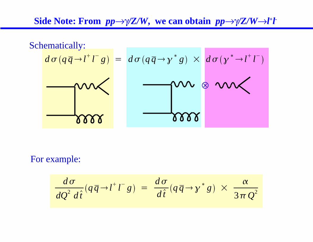
Side Note: From pp→γ/Z/W, we can obtain pp→γ/Z/W→l+l-

d� q q� l� l� g = d� q q��� g × d� ��� l� l�

d�

dQ2 d tq q� l� l� g =

d�d t

q q��� g �

3�Q2

Schematically:

For example:

⊗

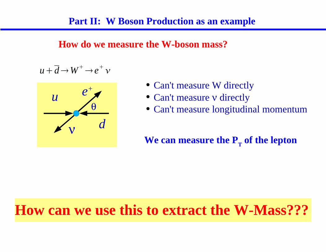
u�d�W�� e��

Part II: W Boson Production as an example

u

d

e+

ν

How do we measure the W-boson mass?

� Can't measure W directly� Can't measure ν directly� Can't measure longitudinal momentum

We can measure the PT of the lepton

How can we use this to extract the W-Mass???

θ

The Jacobian Peak

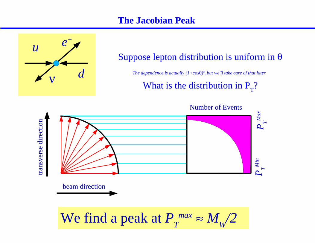
u

d

e+

ν

Suppose lepton distribution is uniform in θThe dependence is actually (1+cosθ)2, but we'll take care of that later

What is the distribution in PT?

beam direction

tran

sver

se d

irec

tion

PT

Max

PT

Min

Number of Events

We find a peak at PT

max ≈ MW/2

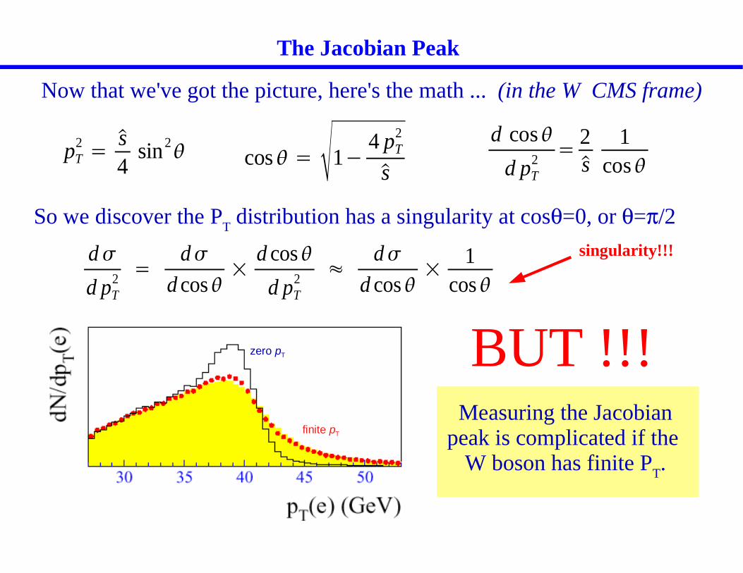
zero pT

finite pT

The Jacobian Peak

Measuring the Jacobian peak is complicated if the

W boson has finite PT.

pT2=

s4

sin2� cos� = 1�

4 pT2

s

d cos�

d pT2 =

2s

1cos�

Now that we've got the picture, here's the math ... (in the W CMS frame)

d�

d pT2 =

d�

d cos�×

d cos�

d pT2 �

d�

d cos�×

1cos�

So we discover the PT distribution has a singularity at cosθ=0, or θ=π/2

BUT !!!

singularity!!!

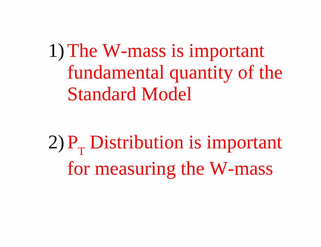
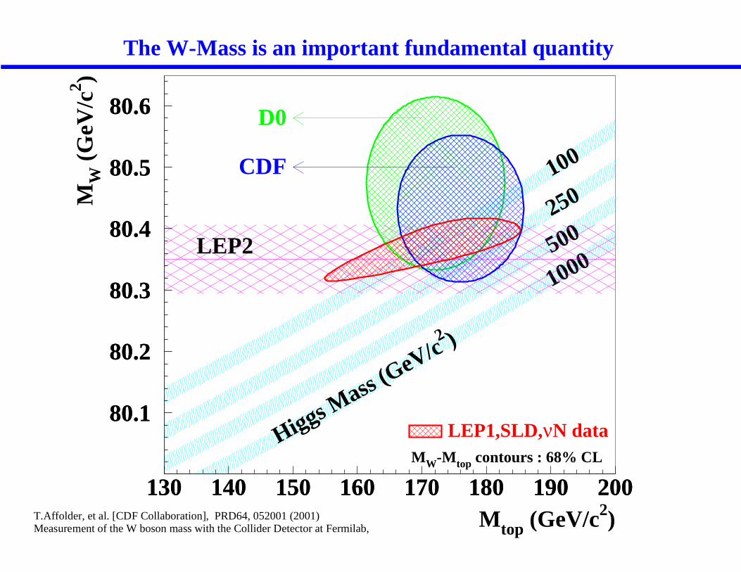
1) The W-mass is important fundamental quantity of the Standard Model

2) PT Distribution is important

for measuring the W-mass

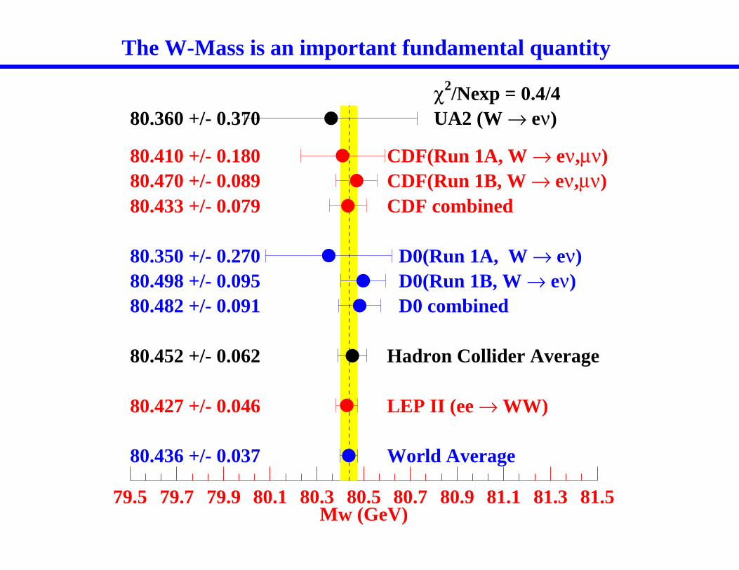
79.5 79.7 79.9 80.1 80.3 80.5 80.7 80.9 81.1 81.3 81.5Mw (GeV)

UA2 (W → eν)

CDF(Run 1A, W → eν,µν)CDF(Run 1B, W → eν,µν)CDF combined

D0(Run 1A, W → eν)D0(Run 1B, W → eν)D0 combined

Hadron Collider Average

LEP II (ee → WW)

World Average

80.360 +/- 0.370

80.410 +/- 0.18080.470 +/- 0.08980.433 +/- 0.079

80.350 +/- 0.27080.498 +/- 0.09580.482 +/- 0.091

80.452 +/- 0.062

80.427 +/- 0.046

80.436 +/- 0.037

χ2/Nexp = 0.4/4

The W-Mass is an important fundamental quantity

80.1

80.2

80.3

80.4

80.5

80.6

130 140 150 160 170 180 190 200Mtop (GeV/c2)

MW

(G

eV/c

2 )

100

250

500

1000

Higgs Mass (

GeV/c2 )

LEP2

D0

CDF

LEP1,SLD,νN dataMW-Mtop contours : 68% CL

80.1

80.2

80.3

80.4

80.5

80.6

130 140 150 160 170 180 190 200T.Affolder, et al. [CDF Collaboration], PRD64, 052001 (2001)Measurement of the W boson mass with the Collider Detector at Fermilab,

The W-Mass is an important fundamental quantity

What gives the W

PT

???

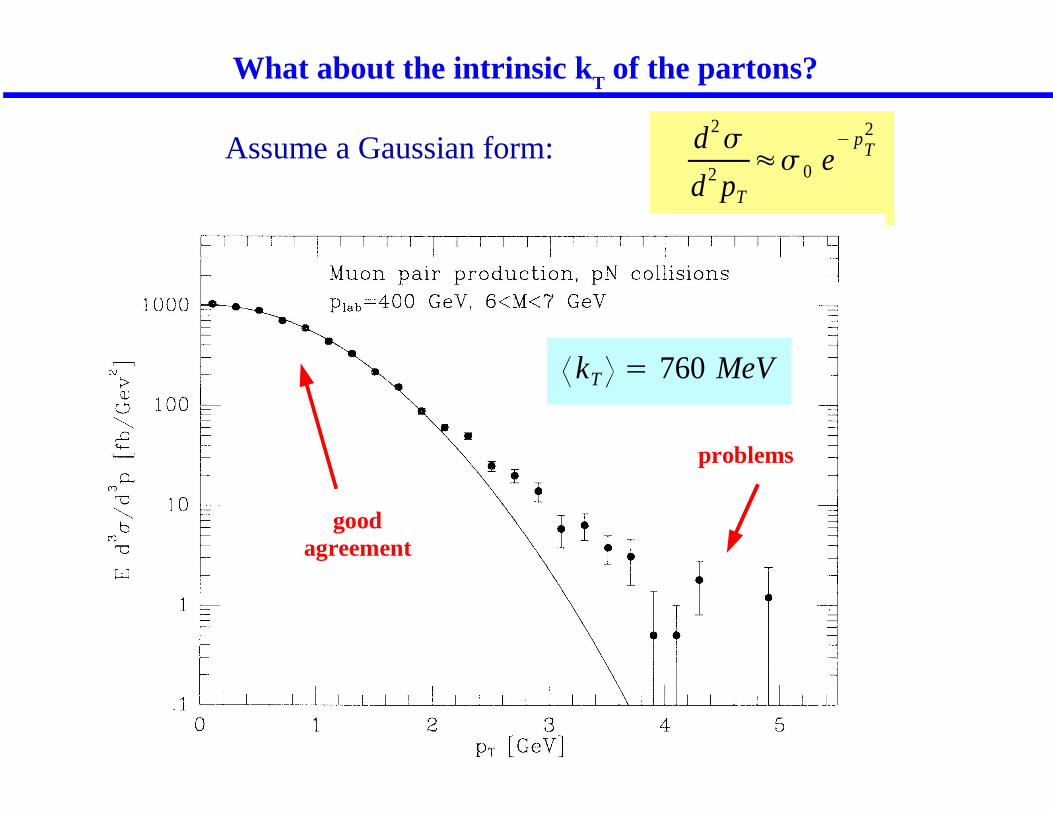
What about the intrinsic kT of the partons?

d2�

d2 pT

�� 0 e� p

T2

kT = 760 MeV

Assume a Gaussian form:

problems

good agreement

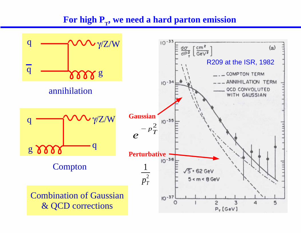
R209 at the ISR, 1982

For high PT, we need a hard parton emission

annihilation

Compton

q

g

γ/Z/W

q

g

q

q

Combination of Gaussian & QCD corrections

e� p

T2

1

pT2

Gaussian

Perturbative

γ/Z/W

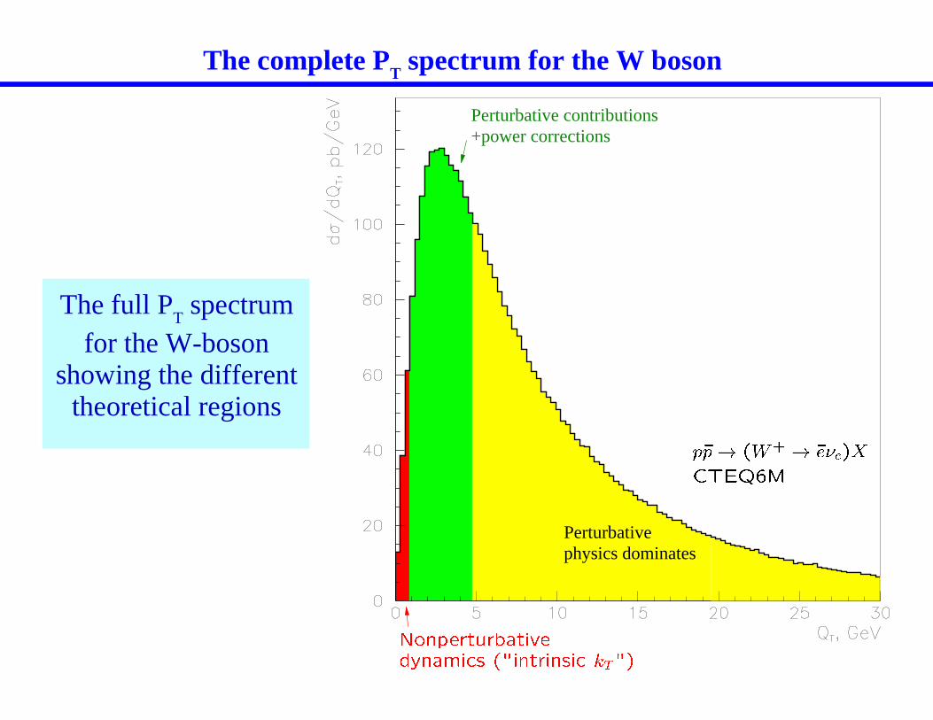
Perturbative contributions+power corrections

Perturbativephysics dominates

p�p! (W+

! �e�e)X

CTEQ6M

Nonperturbative

dynamics ("intrinsic kT")

The complete PT spectrum for the W boson

The full PT spectrum

for the W-boson showing the different

theoretical regions

Road map for Resummation

BEFORE AFTER

⇒

d�

d� dy dpT2 �

d�

d� dy Born

×4� s

3�

ln s / pT2

pT2

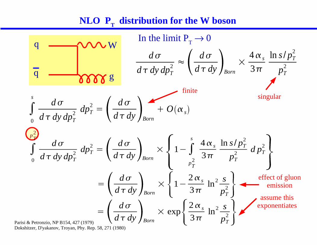
q

g

W

q

NLO PT distribution for the W boson

In the limit PT → 0

�0

sd�

d� dy dpT2 dpT

2=

d�

d� dy Born

� O � s

�0

pT2

d�

d� dy dpT2 dpT

2=

d�

d� dy Born

× 1��p

T2

s4� s

3�

ln s / pT2

pT2 d pT

2

=d�

d� dy Born

× 1�2� s

3�ln2 s

pT2

=d�

d� dy Born

× exp2� s

3�ln2 s

pT2

singularfinite

assume this exponentiates

effect of gluon emission

Parisi & Petronzio, NP B154, 427 (1979)Dokshitzer, D'yakanov, Troyan, Phy. Rep. 58, 271 (1980)

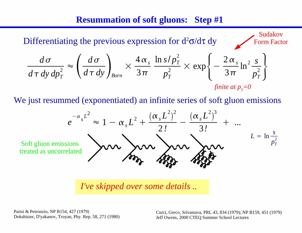
Resummation of soft gluons: Step #1

d�

d� dy dpT2 �

d�

d� dy Born

×4� s

3�

ln s / pT2

pT2 × exp �

2� s

3�ln2 s

pT2

Differentiating the previous expression for d2σ/dτ dy

We just resummed (exponentiated) an infinite series of soft gluon emissions

e��

sL2

� 1 � � s L2�

� s L2 2

2 !�

� s L2 3

3!� ...

Parisi & Petronzio, NP B154, 427 (1979)Dokshitzer, D'yakanov, Troyan, Phy. Rep. 58, 271 (1980)

Soft gluon emissions treated as uncorrelated

Curci, Greco, Srivastava, PRL 43, 834 (1979); NP B159, 451 (1979)Jeff Owens, 2000 CTEQ Summer School Lectures

I've skipped over some details ..

SudakovForm Factor

finite at pT=0

L = lns

pT2

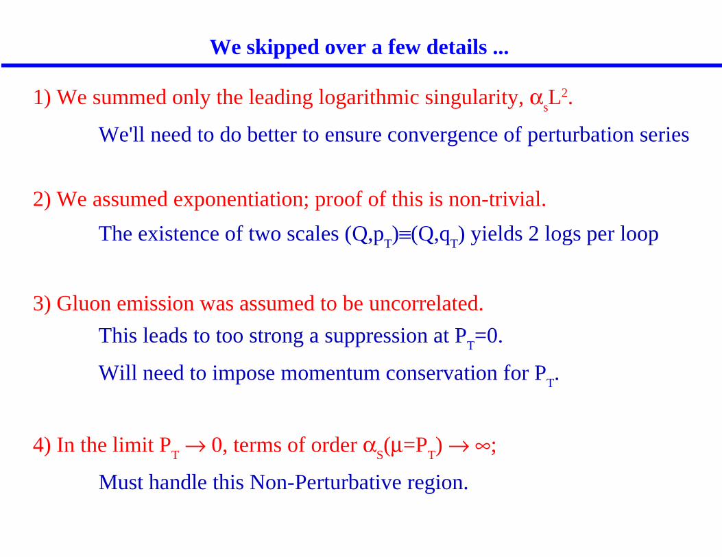
We skipped over a few details ...

1) We summed only the leading logarithmic singularity, αsL2.

We'll need to do better to ensure convergence of perturbation series

2) We assumed exponentiation; proof of this is non-trivial.

The existence of two scales (Q,pT)≡(Q,q

T) yields 2 logs per loop

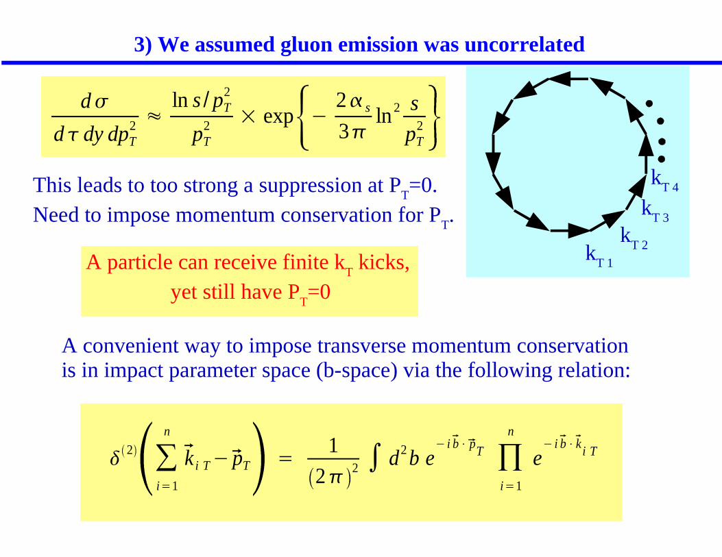
3) Gluon emission was assumed to be uncorrelated.

This leads to too strong a suppression at PT=0.

Will need to impose momentum conservation for PT.

4) In the limit PT → 0, terms of order α

S(µ=P

T) → ∞;

Must handle this Non-Perturbative region.

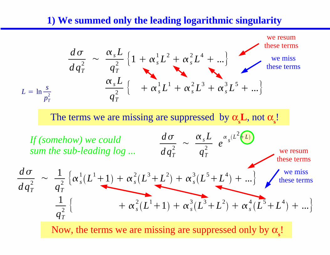
d�

d qT2 ~

� s L

qT2 1 � � s

1 L2� � s

2 L4� ...

� s L

qT2 � � s

1 L1� � s

2 L3� � s

3 L5� ...

we resum these terms

we miss these terms

1) We summed only the leading logarithmic singularity

The terms we are missing are suppressed by αsL, not αs!

d�

d qT2 ~

� s L

qT2 e

�s

L2�LIf (somehow) we could

sum the sub-leading log ...

d�

d qT2 ~

1

qT2 � s

1 L1�1 � � s

2 L3�L2

� � s3 L5

�L4� ...

1

qT2 � � s

2 L1�1 � � s

3 L3�L2

� � s4 L5

�L4� ...

we resum these terms

we miss these terms

Now, the terms we are missing are suppressed only by αs!

L = lns

pT2

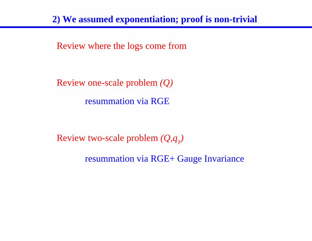
2) We assumed exponentiation; proof is non-trivial

Review where the logs come from

Review one-scale problem (Q)

resummation via RGE

Review two-scale problem (Q,qT)

resummation via RGE+ Gauge Invariance

Where do the

Logs come from?

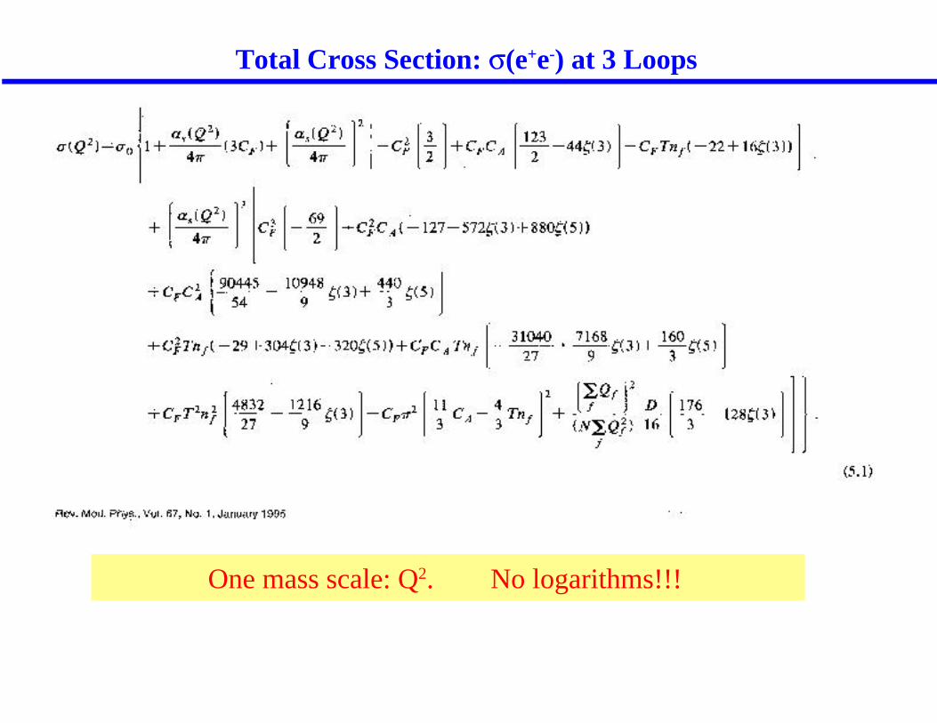
Total Cross Section: σ(e+e-) at 3 Loops

One mass scale: Q2. No logarithms!!!

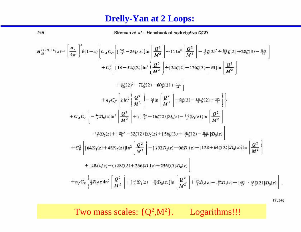
Drelly-Yan at 2 Loops:

Two mass scales: {Q2,M2}. Logarithms!!!

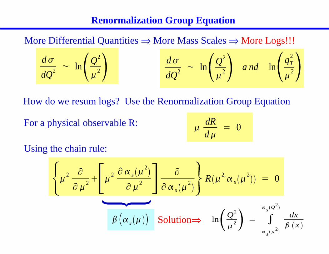
Renormalization Group Equation

More Differential Quantities ⇒ More Mass Scales ⇒ More Logs!!!

d�

dQ2 ~ lnQ2

�2

d�

dQ2~ ln

Q2

�2

a nd lnqT

2

�2

How do we resum logs? Use the Renormalization Group Equation

�dRd�

= 0For a physical observable R:

Using the chain rule:

�2 �

� �2� �

2 � � s �2

� �2

�

� � s �2 R �

2,� s �

2= 0

� � s � lnQ2

�2

= ��

s�

2

�s

Q2

dx� x

Solution⇒

�2 �

� �2� � � s �

�

� � s �2 R �

2,� s �

2= 0

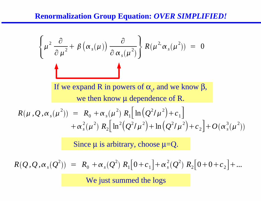
Renormalization Group Equation: OVER SIMPLIFIED!

R � ,Q ,� s �2

= R0 �� s �2 R1 ln Q2

/�2�c1

�� s2�

2 R2 ln2 Q2/�

2� ln Q2

/�2�c2 �O � s

3�

2

If we expand R in powers of αs, and we know β,

we then know µ dependence of R.

Since µ is arbitrary, choose µ=Q.

R Q ,Q ,� s Q2= R0 �� s Q2 R1 0�c1 �� s

2 Q2 R2 0�0�c2 �...

We just summed the logs

d�

d�2=0

d�

d p�� 2=0

� x ,Q2

�2 ,

p�� 2

�2 , ...

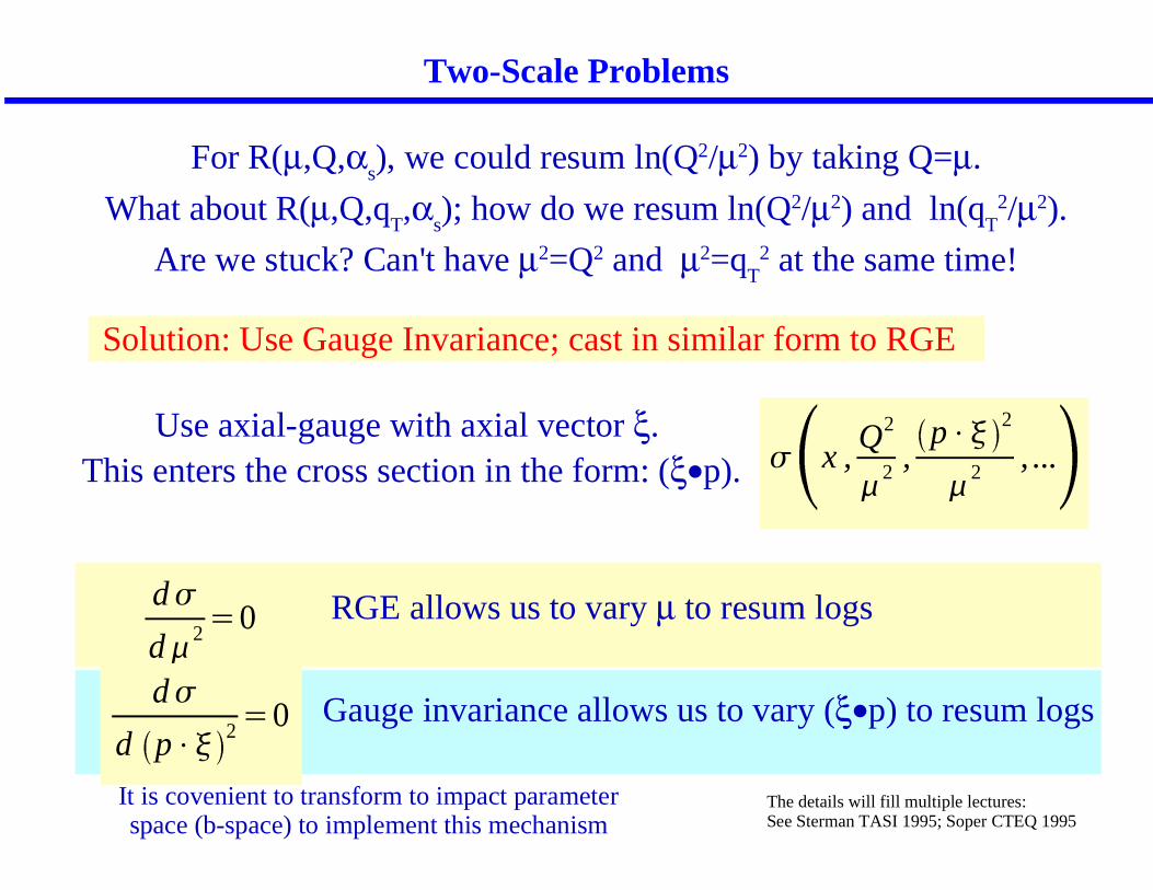
Two-Scale Problems

For R(µ,Q,αs), we could resum ln(Q2/µ2) by taking Q=µ.

What about R(µ,Q,qT,α

s); how do we resum ln(Q2/µ2) and ln(q

T2/µ2).

Are we stuck? Can't have µ2=Q2 and µ2=qT

2 at the same time!

Solution: Use Gauge Invariance; cast in similar form to RGE

Use axial-gauge with axial vector ξ. This enters the cross section in the form: (ξ•p).

RGE allows us to vary µ to resum logs

Gauge invariance allows us to vary (ξ•p) to resum logs

The details will fill multiple lectures: See Sterman TASI 1995; Soper CTEQ 1995

It is covenient to transform to impact parameter space (b-space) to implement this mechanism

3) We assumed gluon emission was uncorrelated

This leads to too strong a suppression at PT=0.

Need to impose momentum conservation for PT.

�2 �

i=1

n

ki T� pT =1

2� 2 � d2 b e� i b� p

T �i=1

n

e� i b�k

i T

A convenient way to impose transverse momentum conservation is in impact parameter space (b-space) via the following relation:

kT 1

kT 2

kT 3

kT 4

A particle can receive finite kT kicks,

yet still have PT=0

d�

d� dy dpT2

ln s / pT2

pT2 × exp �

2 s

3�ln2 s

pT2

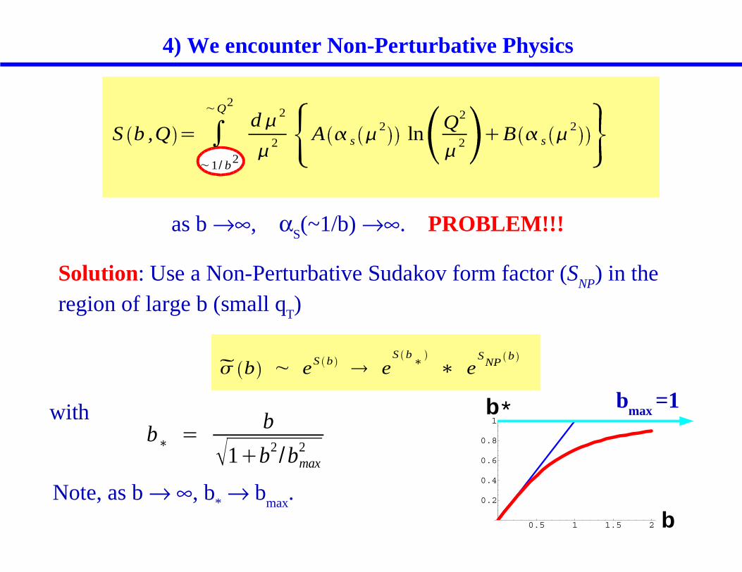
S b ,Q = �~1/ b2

~Q2

d�2

�2 A � s �

2 lnQ2

�2 �B � s �

2

as b →∞, αS(~1/b) →∞. PROBLEM!!!

0.5 1 1.5 2 b0.2

0.4

0.6

0.8

1b*

Solution: Use a Non-Perturbative Sudakov form factor (SNP

) in the region of large b (small q

T)

b� =b

1�b2/bmax

2

� b ~ eS b� e

S b�� e

SNP

b

4) We encounter Non-Perturbative Physics

with

Note, as b → ∞, b* → b

max.

bmax =1

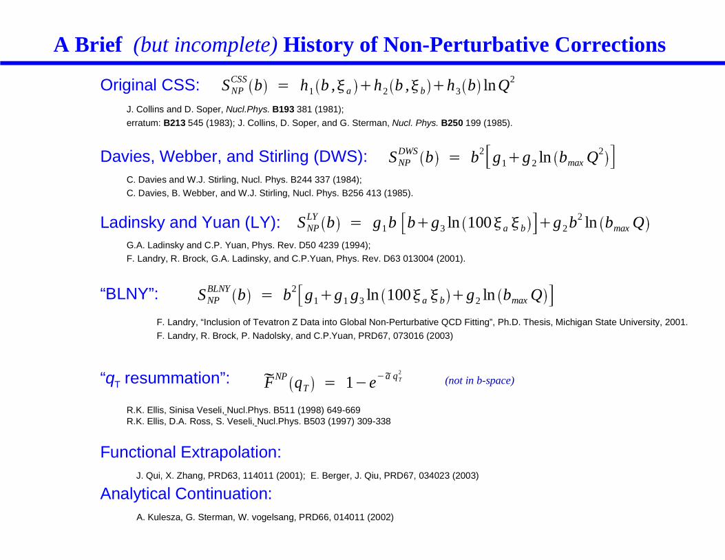
Original CSS:J. Collins and D. Soper, Nucl.Phys. B193 381 (1981);

erratum: B213 545 (1983); J. Collins, D. Soper, and G. Sterman, Nucl. Phys. B250 199 (1985).

Davies, Webber, and Stirling (DWS):C. Davies and W.J. Stirling, Nucl. Phys. B244 337 (1984);

C. Davies, B. Webber, and W.J. Stirling, Nucl. Phys. B256 413 (1985).

Ladinsky and Yuan (LY):G.A. Ladinsky and C.P. Yuan, Phys. Rev. D50 4239 (1994);

F. Landry, R. Brock, G.A. Ladinsky, and C.P.Yuan, Phys. Rev. D63 013004 (2001).

“BLNY”:

F. Landry, “Inclusion of Tevatron Z Data into Global Non-Perturbative QCD Fitting”, Ph.D. Thesis, Michigan State University, 2001.

F. Landry, R. Brock, P. Nadolsky, and C.P.Yuan, PRD67, 073016 (2003)

“qT resummation”:

R.K. Ellis, Sinisa Veseli, Nucl.Phys. B511 (1998) 649-669R.K. Ellis, D.A. Ross, S. Veseli, Nucl.Phys. B503 (1997) 309-338

A Brief (but incomplete) History of Non-Perturbative Corrections

SNPCSS b = h1 b ,�a �h2 b ,�b �h3 b ln Q2

SNPDWS b = b2 g1�g2 ln bmax Q2

SNPLY b = g1b b�g3 ln 100�a �b �g2b2 ln bmax Q

SNPBLNY b = b2 g1�g1 g3 ln 100�a �b �g2 ln bmax Q

FNP qT = 1�e�a qT2

(not in b-space)

Functional Extrapolation:J. Qui, X. Zhang, PRD63, 114011 (2001); E. Berger, J. Qiu, PRD67, 034023 (2003)

Analytical Continuation:A. Kulesza, G. Sterman, W. vogelsang, PRD66, 014011 (2002)

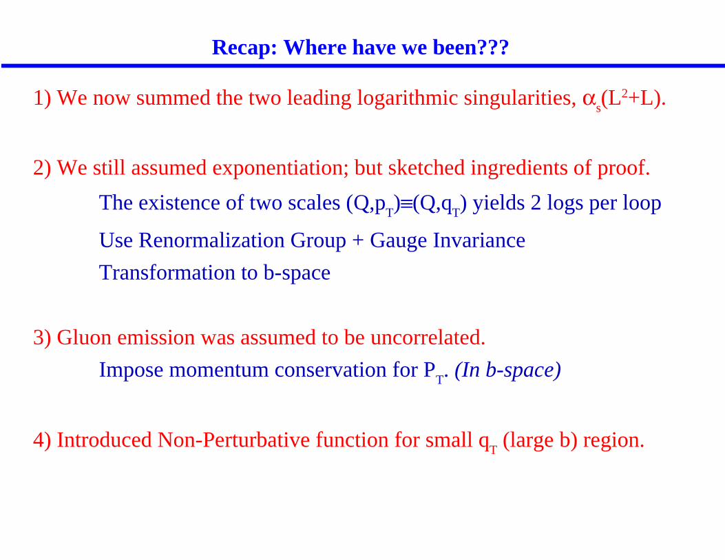
Recap: Where have we been???

1) We now summed the two leading logarithmic singularities, αs(L2+L).

2) We still assumed exponentiation; but sketched ingredients of proof.

The existence of two scales (Q,pT)≡(Q,q

T) yields 2 logs per loop

Use Renormalization Group + Gauge Invariance

Transformation to b-space

3) Gluon emission was assumed to be uncorrelated.

Impose momentum conservation for PT. (In b-space)

4) Introduced Non-Perturbative function for small qT (large b) region.

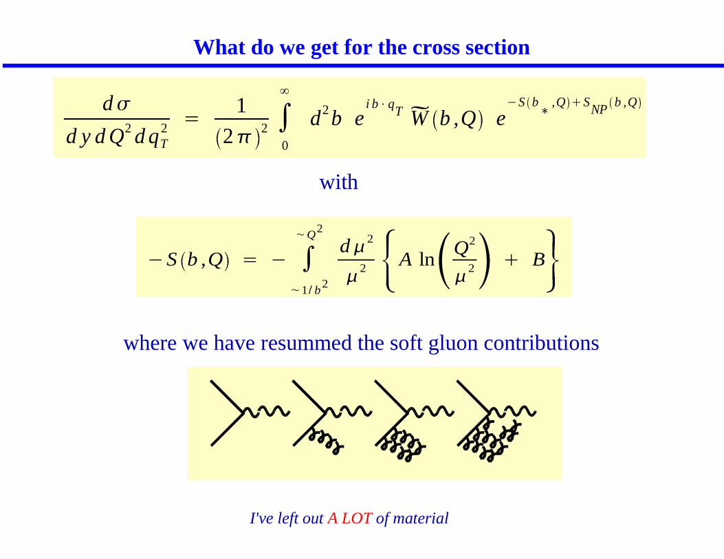
d�

d y d Q2 d qT2 =

1

2� 2 �0

�

d2 b ei b�q

T W b ,Q e�S b

�,Q �S

NPb ,Q

What do we get for the cross section

�S b ,Q = � �~1/ b2

~Q2

d�2

�2 A ln

Q2

�2 � B

with

I've left out A LOT of material

where we have resummed the soft gluon contributions

d�

d qT2 ~

� s L

qT2 e

�s

L2�L

~

1

qT2 � s L � � s

2 L3�L2

�...

d� resum ~ � s L � � s2 L3

�L2� 0�0 � � s

3 L5�L4

�...

d� pert ~ � s L � � s2 L3

�L2�L1

�1 � � s3 0�0

d� asym ~ � s L � � s2 L3

�L2� 0�0 � � s

3 0�0

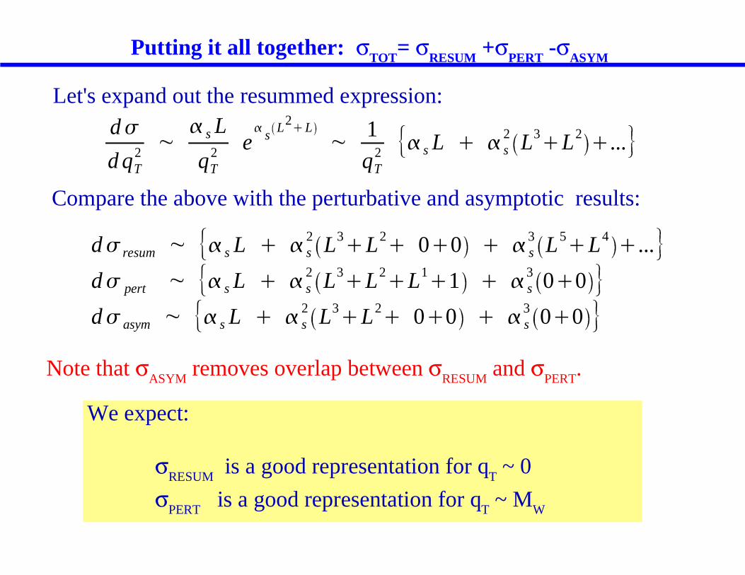
Putting it all together: σTOT= σRESUM +σPERT -σASYM

Let's expand out the resummed expression:

Compare the above with the perturbative and asymptotic results:

Note that σASYM

removes overlap between σRESUM

and σPERT

.

We expect:

σRESUM

is a good representation for qT ~ 0

σPERT is a good representation for qT ~ MW

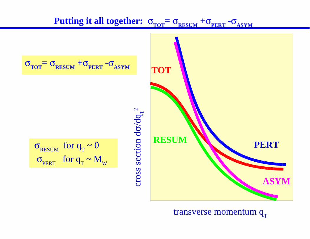
Putting it all together: σTOT= σRESUM +σPERT -σASYM

RESUM PERT

TOT

ASYM

σRESUM

for qT ~ 0

σPERT for qT ~ MW

cros

s se

ctio

n dσ

/dq T

2

transverse momentum qT

σTOT= σRESUM +σPERT -σASYM

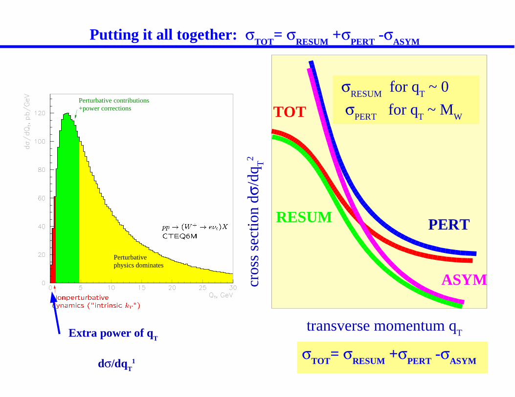
Putting it all together: σTOT= σRESUM +σPERT -σASYM

RESUM PERT

TOT

ASYM

σRESUM

for qT ~ 0

σPERT for qT ~ MW

cros

s se

ctio

n dσ

/dq T

2

transverse momentum qT

σTOT= σRESUM +σPERT -σASYM

Perturbative contributions+power corrections

Perturbativephysics dominates

p�p! (W+

! �e�e)X

CTEQ6M

Nonperturbative

dynamics ("intrinsic kT")

Extra power of qT

dσ/dqT

1

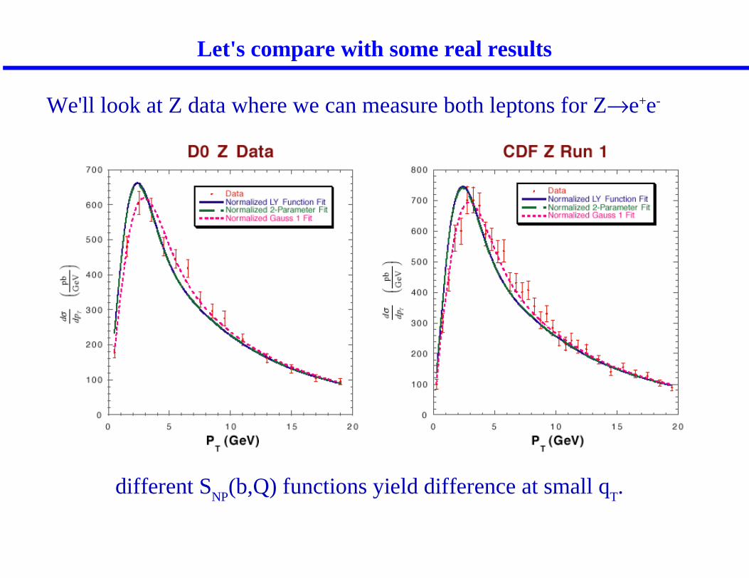
Let's compare with some real results

We'll look at Z data where we can measure both leptons for Z→e+e-

different SNP

(b,Q) functions yield difference at small qT.

Let's return

to the

measurement

of MW

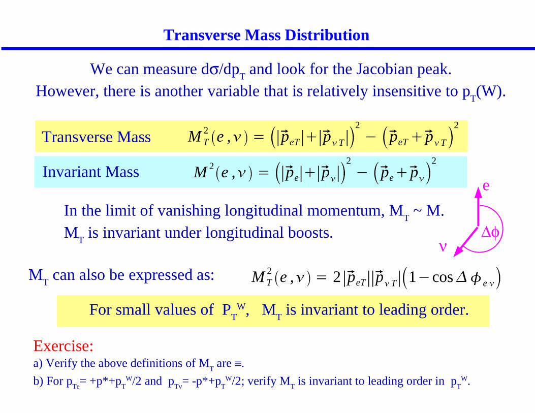
Transverse Mass Distribution

We can measure dσ/dpT and look for the Jacobian peak.

However, there is another variable that is relatively insensitive to pT(W).

M T2 e ,� = peT � p

�T

2

� peT�p�T

2

M 2 e ,� = pe � p�

2

� pe�p�

2

Transverse Mass

Invariant Mass

In the limit of vanishing longitudinal momentum, MT ~ M.

MT is invariant under longitudinal boosts.

M T2 e ,� = 2 peT p

�T 1�cos�� e �M

T can also be expressed as:

For small values of PT

W, MT is invariant to leading order.

Exercise: a) Verify the above definitions of M

T are ≡.

b) For pTe

= +p*+pT

W/2 and pTν= -p*+p

TW/2; verify M

T is invariant to leading order in p

TW.

e

ν∆φ

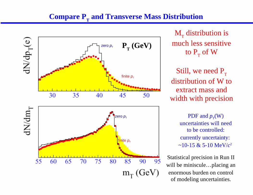
Compare PT and Transverse Mass Distribution

zero pT

finite pT

zero pT

finite pT

PT (GeV)

MT distribution is

much less sensitive to PT of W

Still, we need PT

distribution of W to extract mass and

width with precision

Statistical precision in Run IIwill be miniscule…placing anenormous burden on control of modeling uncertainties.

PDF and pT(W) uncertainties will need

to be controlled:currently uncertainty:

~10-15 & 5-10 MeV/c2

The Future:Tevatron Run II ... happening now

LHC ... happening soon

0

500

1000

1500

2000

50 60 70 80 90 100 110 120

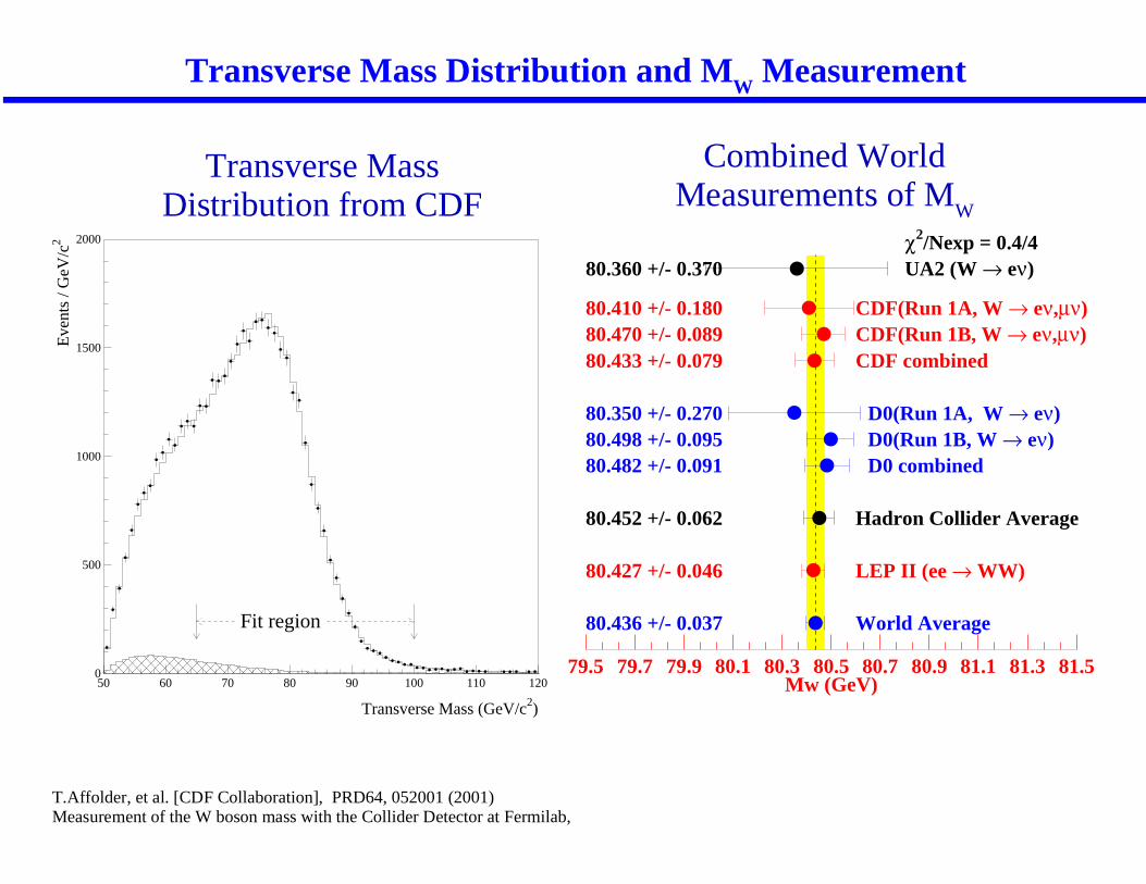
Fit region

Transverse Mass (GeV/c2)

Eve

nts

/ GeV

/c2

Transverse Mass Distribution and MW Measurement

T.Affolder, et al. [CDF Collaboration], PRD64, 052001 (2001)Measurement of the W boson mass with the Collider Detector at Fermilab,

79.5 79.7 79.9 80.1 80.3 80.5 80.7 80.9 81.1 81.3 81.5Mw (GeV)

UA2 (W → eν)

CDF(Run 1A, W → eν,µν)CDF(Run 1B, W → eν,µν)CDF combined

D0(Run 1A, W → eν)D0(Run 1B, W → eν)D0 combined

Hadron Collider Average

LEP II (ee → WW)

World Average

80.360 +/- 0.370

80.410 +/- 0.18080.470 +/- 0.08980.433 +/- 0.079

80.350 +/- 0.27080.498 +/- 0.09580.482 +/- 0.091

80.452 +/- 0.062

80.427 +/- 0.046

80.436 +/- 0.037

χ2/Nexp = 0.4/4

Transverse Mass Distribution from CDF

Combined World Measurements of M

W

��

25 30 35 40 45 50 55 60 65 70 75

0

100

200

300

400

500

600

0 10 20 30 40 50 60

0

100

200

300

400

500

600

700

800

25 30 35 40 45 50 55 60 65 70 75

0

100

200

300

400

500

600

30 40 50 60 70 80 90 100 110 120

0

100

200

300

400

500

ET

/GeV

T/GeVM

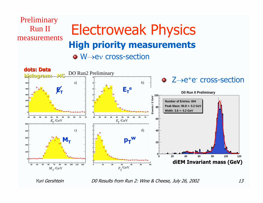
DO Run2 Preliminary

ET

/GeV

pT/GeV

a)

c)

b)

d)

Di-Electron Mass (GeV)0 20 40 60 80 100 120

Ev

en

ts/

2G

eV

0

20

40

60

80

100

Number of Entries: 604

Peak Mass: 90.8 +- 0.2 GeV

Width: 3.6 +- 0.2 GeV

D0 Run II Preliminary

�

Preliminary Run II

measurements

80.1

80.2

80.3

80.4

80.5

80.6

130 140 150 160 170 180 190 200Mtop (GeV/c2)

MW

(G

eV/c

2 )

100

250

500

1000

Higgs Mass (

GeV/c2 )

LEP2

D0

CDF

LEP1,SLD,νN dataMW-Mtop contours : 68% CL

80.1

80.2

80.3

80.4

80.5

80.6

130 140 150 160 170 180 190 200T.Affolder, et al. [CDF Collaboration], PRD64, 052001 (2001)Measurement of the W boson mass with the Collider Detector at Fermilab,

The W-Mass is an important fundamental quantity

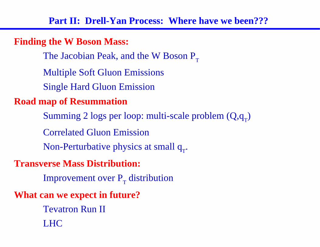
Part II: Drell-Yan Process: Where have we been???

Finding the W Boson Mass:

The Jacobian Peak, and the W Boson PT

Multiple Soft Gluon Emissions

Single Hard Gluon Emission

Road map of Resummation

Summing 2 logs per loop: multi-scale problem (Q,qT)

Correlated Gluon Emission

Non-Perturbative physics at small qT.

Transverse Mass Distribution:

Improvement over PT distribution

What can we expect in future?

Tevatron Run II

LHC

Thanks to ...

Jeff Owens

Chip Brock

C.P. Yuan

Pavel Nadolsky

Randy Scalise

Wu-Ki Tung

Steve Kuhlmann

Dave Soper

and my other CTEQ colleagues

and the many web pages where I borrowed my figures ...

References:

Ellis, Webber, Stirling

Barger & Phillips, 2nd Edition

Rick Field; Perturbative QCD

CTEQ HandbookCTEQ Pedagogical Page:

CTEQ Lectures:C.P. Yuan, 2002Chip Brock, 2001Jeff Owens, 2000

Attention:

You have reached the very last page of the internet.

We hope you enjoyed your browsing.

Now turn off your computer and go out and play.calculate