
Fractional hot deck imputation - Jae Kim
35
Fractional hot deck imputation for multivariate missing data in survey sampling Jae Kwang Kim 1 Iowa State University March 18, 2015 1 Joint work with Jongho Im and Wayne Fuller
-
Upload
jae-kwang-kim -
Category
Education
-
view
48 -
download
2
Transcript of Fractional hot deck imputation - Jae Kim
Fractional hot deck imputation for multivariatemissing data in survey sampling
Jae Kwang Kim 1
Iowa State University
March 18, 2015
1Joint work with Jongho Im and Wayne Fuller
IntroductionBasic Setup
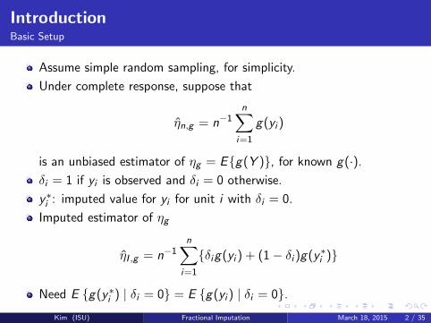
Assume simple random sampling, for simplicity.
Under complete response, suppose that
η̂n,g = n−1n∑
i=1
g(yi )
is an unbiased estimator of ηg = E{g(Y )}, for known g(·).
δi = 1 if yi is observed and δi = 0 otherwise.
y∗i : imputed value for yi for unit i with δi = 0.
Imputed estimator of ηg
η̂I ,g = n−1n∑
i=1
{δig(yi ) + (1− δi )g(y∗i )}
Need E {g(y∗i ) | δi = 0} = E {g(yi ) | δi = 0}.Kim (ISU) Fractional Imputation March 18, 2015 2 / 35
IntroductionML estimation under missing data setup
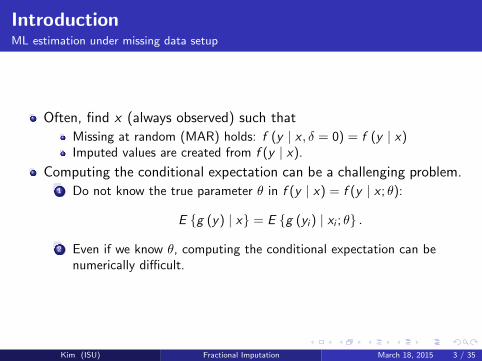
Often, find x (always observed) such that
Missing at random (MAR) holds: f (y | x , δ = 0) = f (y | x)Imputed values are created from f (y | x).
Computing the conditional expectation can be a challenging problem.1 Do not know the true parameter θ in f (y | x) = f (y | x ; θ):
E {g (y) | x} = E {g (yi ) | xi ; θ} .
2 Even if we know θ, computing the conditional expectation can benumerically difficult.
Kim (ISU) Fractional Imputation March 18, 2015 3 / 35
IntroductionImputation
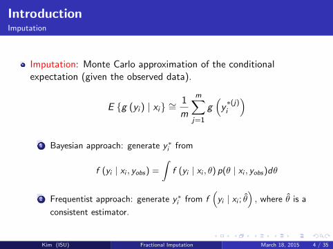
Imputation: Monte Carlo approximation of the conditionalexpectation (given the observed data).
E {g (yi ) | xi} ∼=1
m
m∑j=1
g(y∗(j)i
)
1 Bayesian approach: generate y∗i from
f (yi | xi , yobs) =
∫f (yi | xi , θ) p(θ | xi , yobs)dθ
2 Frequentist approach: generate y∗i from f(yi | xi ; θ̂
), where θ̂ is a
consistent estimator.
Kim (ISU) Fractional Imputation March 18, 2015 4 / 35
IntroductionBasic Setup (Cont’d)
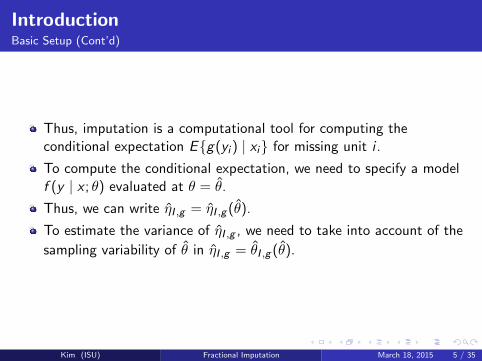
Thus, imputation is a computational tool for computing theconditional expectation E{g(yi ) | xi} for missing unit i .
To compute the conditional expectation, we need to specify a modelf (y | x ; θ) evaluated at θ = θ̂.
Thus, we can write η̂I ,g = η̂I ,g (θ̂).
To estimate the variance of η̂I ,g , we need to take into account of the
sampling variability of θ̂ in η̂I ,g = θ̂I ,g (θ̂).
Kim (ISU) Fractional Imputation March 18, 2015 5 / 35
IntroductionBasic Setup (Cont’d)
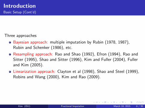
Three approaches
Bayesian approach: multiple imputation by Rubin (1978, 1987),Rubin and Schenker (1986), etc.
Resampling approach: Rao and Shao (1992), Efron (1994), Rao andSitter (1995), Shao and Sitter (1996), Kim and Fuller (2004), Fullerand Kim (2005).
Linearization approach: Clayton et al (1998), Shao and Steel (1999),Robins and Wang (2000), Kim and Rao (2009).
Kim (ISU) Fractional Imputation March 18, 2015 6 / 35
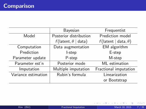
Comparison
Bayesian Frequentist
Model Posterior distribution Prediction modelf (latent, θ | data) f (latent | data, θ)
Computation Data augmentation EM algorithmPrediction I-step E-step
Parameter update P-step M-step
Parameter est’n Posterior mode ML estimation
Imputation Multiple imputation Fractional imputation
Variance estimation Rubin’s formula Linearizationor Bootstrap
Kim (ISU) Fractional Imputation March 18, 2015 7 / 35
Multiple imputation
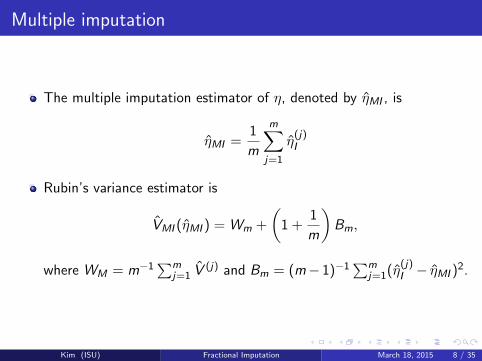
The multiple imputation estimator of η, denoted by η̂MI , is
η̂MI =1
m
m∑j=1
η̂(j)I
Rubin’s variance estimator is
V̂MI (η̂MI ) = Wm +
(1 +
1
m
)Bm,
where WM = m−1∑m
j=1 V̂(j) and Bm = (m− 1)−1
∑mj=1(η̂
(j)I − η̂MI )
2.
Kim (ISU) Fractional Imputation March 18, 2015 8 / 35
Multiple imputation
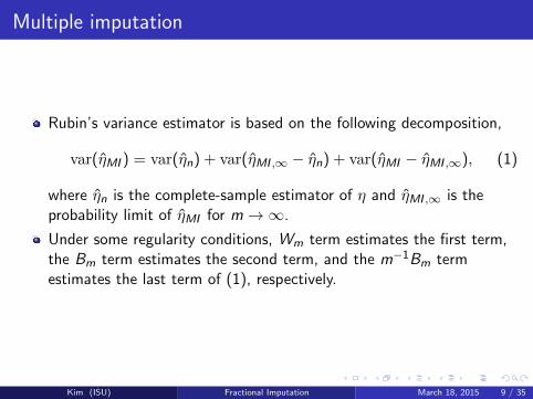
Rubin’s variance estimator is based on the following decomposition,
var(η̂MI ) = var(η̂n) + var(η̂MI ,∞ − η̂n) + var(η̂MI − η̂MI ,∞), (1)
where η̂n is the complete-sample estimator of η and η̂MI ,∞ is theprobability limit of η̂MI for m→∞.
Under some regularity conditions, Wm term estimates the first term,the Bm term estimates the second term, and the m−1Bm termestimates the last term of (1), respectively.
Kim (ISU) Fractional Imputation March 18, 2015 9 / 35

Multiple imputation
In particular, Kim et al (2006, JRSSB) proved that the bias ofRubin’s variance estimator is
Bias(V̂MI ) ∼= −2cov(η̂MI − η̂n, η̂n). (2)
The decomposition (1) is equivalent to assuming thatcov(η̂MI − η̂n, η̂n) ∼= 0, which is called the congeniality condition byMeng (1994).
The congeniality condition holds when η̂n is the MLE of η. In suchcases, Rubin’s variance estimator is asymptotically unbiased.
Kim (ISU) Fractional Imputation March 18, 2015 10 / 35
Multiple imputation
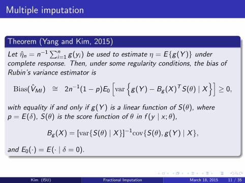
Theorem (Yang and Kim, 2015)
Let η̂n = n−1∑n
i=1 g(yi ) be used to estimate η = E{g(Y )} undercomplete response. Then, under some regularity conditions, the bias ofRubin’s variance estimator is
Bias(V̂MI ) ∼= 2n−1(1− p)E0
[var{g(Y )− Bg (X )TS(θ) | X
}]≥ 0,
with equality if and only if g(Y ) is a linear function of S(θ), wherep = E (δ), S(θ) is the score function of θ in f (y | x ; θ),
Bg (X ) = [var{S(θ) | X}]−1cov{S(θ), g(Y ) | X},
and E0(·) = E (· | δ = 0).
Kim (ISU) Fractional Imputation March 18, 2015 11 / 35
Multiple imputation
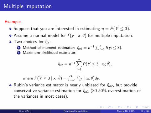
Example
Suppose that you are interested in estimating η = P(Y ≤ 3).
Assume a normal model for f (y | x ; θ) for multiple imputation.
Two choices for η̂n:1 Method-of-moment estimator: η̂n1 = n−1
∑ni=1 I (yi ≤ 3).
2 Maximum-likelihood estimator:
η̂n2 = n−1n∑
i=1
P(Y ≤ 3 | xi ; θ̂),
where P(Y ≤ 3 | xi ; θ̂) =∫ 3
−∞ f (y | xi ; θ)dy .
Rubin’s variance estimator is nearly unbiased for η̂n2, but provideconservative variance estimation for η̂n1 (30-50% overestimation ofthe variances in most cases).
Kim (ISU) Fractional Imputation March 18, 2015 12 / 35
Fractional Imputation
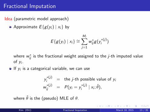
Idea (parametric model approach)
Approximate E{g(yi ) | xi} by
E{g(yi ) | xi} ∼=Mi∑j=1
w∗ij g(y∗(j)i )
where w∗ij is the fractional weight assigned to the j-th imputed valueof yi .
If yi is a categorical variable, we can use
y∗(j)i = the j-th possible value of yi
w∗(j)ij = P(yi = y
∗(j)i | xi ; θ̂),
where θ̂ is the (pseudo) MLE of θ.
Kim (ISU) Fractional Imputation March 18, 2015 13 / 35
Fractional imputation
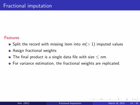
Features
Split the record with missing item into m(> 1) imputed values
Assign fractional weights
The final product is a single data file with size ≤ nm.
For variance estimation, the fractional weights are replicated.
Kim (ISU) Fractional Imputation March 18, 2015 14 / 35
Fractional imputation
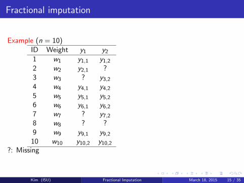
Example (n = 10)ID Weight y1 y21 w1 y1,1 y1,22 w2 y2,1 ?3 w3 ? y3,24 w4 y4,1 y4,25 w5 y5,1 y5,26 w6 y6,1 y6,27 w7 ? y7,28 w8 ? ?9 w9 y9,1 y9,2
10 w10 y10,2 y10,2?: Missing
Kim (ISU) Fractional Imputation March 18, 2015 15 / 35
Fractional imputation (categorical case)
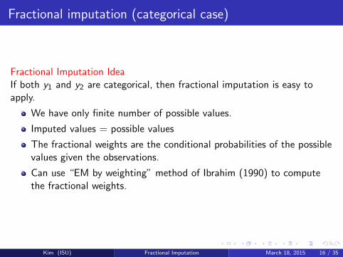
Fractional Imputation IdeaIf both y1 and y2 are categorical, then fractional imputation is easy toapply.
We have only finite number of possible values.
Imputed values = possible values
The fractional weights are the conditional probabilities of the possiblevalues given the observations.
Can use “EM by weighting” method of Ibrahim (1990) to computethe fractional weights.
Kim (ISU) Fractional Imputation March 18, 2015 16 / 35
Fractional imputation (categorical case)
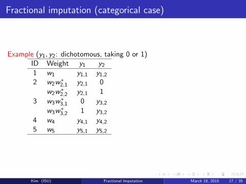
Example (y1, y2: dichotomous, taking 0 or 1)ID Weight y1 y21 w1 y1,1 y1,22 w2w
∗2,1 y2,1 0
w2w∗2,2 y2,1 1
3 w3w∗3,1 0 y3,2
w3w∗3,2 1 y3,2
4 w4 y4,1 y4,25 w5 y5,1 y5,2
Kim (ISU) Fractional Imputation March 18, 2015 17 / 35
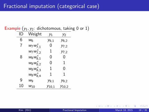
Fractional imputation (categorical case)
Example (y1, y2: dichotomous, taking 0 or 1)ID Weight y1 y26 w6 y6,1 y6,27 w7w
∗7,1 0 y7,2
w7w∗7,2 1 y7,2
8 w8w∗8,1 0 0
w8w∗8,2 0 1
w8w∗8,3 1 0
w8w∗8,4 1 1
9 w9 y9,1 y9,210 w10 y10,1 y10,2
Kim (ISU) Fractional Imputation March 18, 2015 18 / 35
Fractional imputation (categorical case)
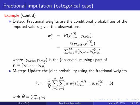
Example (Cont’d)
E-step: Fractional weights are the conditional probabilities of theimputed values given the observations.
w∗ij = P̂(y∗(j)i ,mis | yi ,obs)
=π̂(yi ,obs , y
∗(j)i ,mis)∑Mi
l=1 π̂(yi ,obs , y∗(l)i ,mis)
where (yi ,obs , yi ,mis) is the (observed, missing) part ofyi = (yi1, · · · , yi ,p).
M-step: Update the joint probability using the fractional weights.
π̂ab =1
N̂
n∑i=1
Mi∑j=1
wiw∗ij I (y
∗(j)i ,1 = a, y
∗(j)i ,2 = b)
with N̂ =∑n
i=1 wi .
Kim (ISU) Fractional Imputation March 18, 2015 19 / 35
Fractional imputation (categorical case)
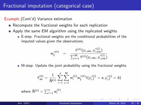
Example (Cont’d) Variance estimation
Recompute the fractional weights for each replication
Apply the same EM algorithm using the replicated weights.
E-step: Fractional weights are the conditional probabilities of theimputed values given the observations.
w∗(k)ij =
π̂(k)(yi,obs , y∗(j)i,mis)∑Mi
l=1 π̂(k)(yi,obs , y
∗(l)i,mis)
M-step: Update the joint probability using the fractional weights.
π̂(k)ab =
1
N̂(k)
n∑i=1
Mi∑j=1
w(k)i w
∗(k)ij I (y
∗(j)i,1 = a, y
∗(j)i,2 = b)
where N̂(k) =∑n
i=1 w(k)i .
Kim (ISU) Fractional Imputation March 18, 2015 20 / 35
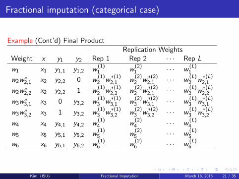
Fractional imputation (categorical case)
Example (Cont’d) Final ProductReplication Weights
Weight x y1 y2 Rep 1 Rep 2 · · · Rep L
w1 x1 y1,1 y1,2 w(1)1 w
(2)1 · · · w
(L)1
w2w∗2,1 x2 y2,2 0 w
(1)2 w
∗(1)2,1 w
(2)2 w
∗(2)2,1 · · · w
(L)2 w
∗(L)2,1
w2w∗2,2 x2 y2,2 1 w
(1)2 w
∗(1)2,2 w
(2)2 w
∗(2)2,1 · · · w
(L)2 w
∗(L)2,2
w3w∗3,1 x3 0 y3,2 w
(1)3 w
∗(1)3,1 w
(2)3 w
∗(2)3,1 · · · w
(L)3 w
∗(L)3,1
w3w∗3,2 x3 1 y3,2 w
(1)3 w
∗(1)3,2 w
(2)3 w
∗(2)3,2 · · · w
(L)3 w
∗(L)3,2
w4 x4 y4,1 y4,2 w(1)4 w
(2)4 · · · w
(L)4
w5 x5 y5,1 y5,2 w(1)5 w
(2)5 · · · w
(L)5
w6 x6 y6,1 y6,2 w(1)6 w
(2)6 · · · w
(L)6
Kim (ISU) Fractional Imputation March 18, 2015 21 / 35
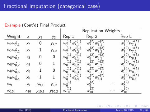
Fractional imputation (categorical case)
Example (Cont’d) Final ProductReplication Weights
Weight x y1 y2 Rep 1 Rep 2 Rep L
w7w∗7,1 x7 0 y7,2 w
(1)7 w
∗(1)7,1 w
(2)7 w
∗(2)7,1 w
(L)7 w
∗(L)7,1
w7w∗7,2 x7 1 y7,2 w
(1)7 w
∗(1)7,2 w
(2)7 w
∗(2)7,2 w
(L)7 w
∗(L)7,2
w8w∗8,1 x8 0 0 w
(1)8 w
∗(1)8,1 w
(2)8 w
∗(2)8,1 w
(L)8 w
∗(L)8,1
w8w∗8,2 x8 0 1 w
(1)8 w
∗(1)8,2 w
(2)8 w
∗(2)8,2 w
(L)8 w
∗(L)8,2
w8w∗8,3 x8 1 0 w
(1)8 w
∗(1)8,3 w
(2)8 w
∗(2)8,3 w
(L)8 w
∗(L)8,3
w8w∗8,4 x8 1 1 w
(1)8 w
∗(1)8,4 w
(2)8 w
∗(2)8,4 w
(L)8 w
∗(L)8,4
w9 x9 y9,1 y9,2 w(1)9 w
(2)9 · · · w
(L)9
w10 x10 y10,1 y10,2 w(1)10 w
(2)10 · · · w
(L)10
Kim (ISU) Fractional Imputation March 18, 2015 22 / 35
Fractional hot deck imputation (general case)
Goals
Fractional hot deck imputation of size m. The final product is asingle data file with size ≤ n ·m.
Preserves correlation structure
Variance estimation relatively easy
Can handle domain estimation (but we do not know which domainswill be used.)
Kim (ISU) Fractional Imputation March 18, 2015 23 / 35
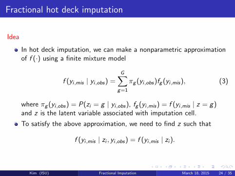
Fractional hot deck imputation
Idea
In hot deck imputation, we can make a nonparametric approximationof f (·) using a finite mixture model
f (yi ,mis | yi ,obs) =G∑
g=1
πg (yi ,obs)fg (yi ,mis), (3)
where πg (yi ,obs) = P(zi = g | yi ,obs), fg (yi ,mis) = f (yi ,mis | z = g)and z is the latent variable associated with imputation cell.
To satisfy the above approximation, we need to find z such that
f (yi ,mis | zi , yi ,obs) = f (yi ,mis | zi ).
Kim (ISU) Fractional Imputation March 18, 2015 24 / 35
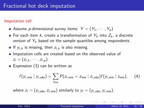
Fractional hot deck imputation
Imputation cell
Assume p-dimensional survey items: Y = (Y1, · · · ,Yp)
For each item k, create a transformation of Yk into Zk , a discreteversion of Yk based on the sample quantiles among respondents.
If yi ,k is missing, then zi ,k is also missing.
Imputation cells are created based on the observed value ofzi = (zi ,1, · · · , zi ,p).
Expression (3) can be written as
f (yi ,mis | yi ,obs) =∑zmis
P(zi ,mis = zmis | zi ,obs)f (yi ,mis | zmis), (4)
where zi = (zi ,obs , zi ,mis) similarly to yi = (yi ,obs , yi ,mis).
Kim (ISU) Fractional Imputation March 18, 2015 25 / 35
Fractional hot deck imputation
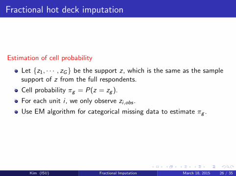
Estimation of cell probability
Let {z1, · · · , zG} be the support z , which is the same as the samplesupport of z from the full respondents.
Cell probability πg = P(z = zg ).
For each unit i , we only observe zi ,obs .
Use EM algorithm for categorical missing data to estimate πg .
Kim (ISU) Fractional Imputation March 18, 2015 26 / 35
Fractional hot deck imputation
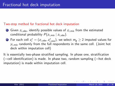
Two-step method for fractional hot deck imputation
1 Given zi ,obs , identify possible values of zi ,mis from the estimatedconditional probability P(zi ,mis | zi ,obs).
2 For each cell z∗i = (zi ,obs , z∗i ,mis), we select mg ≥ 2 imputed values for
yi ,mis randomly from the full respondents in the same cell. (Joint hotdeck within imputation cell)
It is essentially two-phase stratified sampling. In phase one, stratification(=cell identification) is made. In phase two, random sampling (=hot deckimputation) is made within imputation cell.
Kim (ISU) Fractional Imputation March 18, 2015 27 / 35
Fractional hot deck imputation
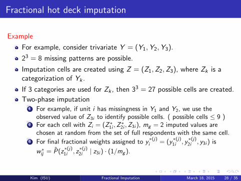
Example
For example, consider trivariate Y = (Y1,Y2,Y3).
23 = 8 missing patterns are possible.
Imputation cells are created using Z = (Z1,Z2,Z3), where Zk is acategorization of Yk .
If 3 categories are used for Zk , then 33 = 27 possible cells are created.
Two-phase imputation1 For example, if unit i has missingness in Y1 and Y2, we use the
observed value of Z3i to identify possible cells. ( possible cells ≤ 9 )2 For each cell with Zi = (Z∗1i ,Z
∗2i ,Z3i ), mg = 2 imputed values are
chosen at random from the set of full respondents with the same cell.3 For final fractional weights assigned to y
∗(j)i = (y
∗(j)1i , y
∗(j)2i , y3i ) is
w∗ij = P̂(z∗(j)1i , z
∗(j)2i | z3i ) · (1/mg ).
Kim (ISU) Fractional Imputation March 18, 2015 28 / 35
Variance estimation
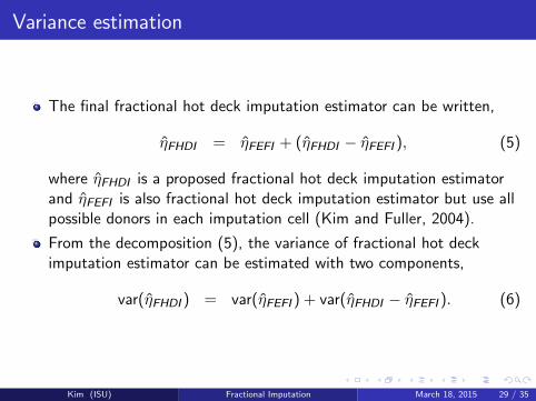
The final fractional hot deck imputation estimator can be written,
η̂FHDI = η̂FEFI + (η̂FHDI − η̂FEFI ), (5)
where η̂FHDI is a proposed fractional hot deck imputation estimatorand η̂FEFI is also fractional hot deck imputation estimator but use allpossible donors in each imputation cell (Kim and Fuller, 2004).
From the decomposition (5), the variance of fractional hot deckimputation estimator can be estimated with two components,
var(η̂FHDI ) = var(η̂FEFI ) + var(η̂FHDI − η̂FEFI ). (6)
Kim (ISU) Fractional Imputation March 18, 2015 29 / 35
Variance estimation (Cont’d)
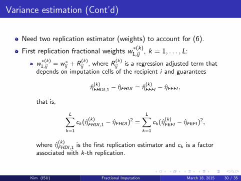
Need two replication estimator (weights) to account for (6).
First replication fractional weights w∗(k)1,ij , k = 1, . . . , L:
w∗(k)1,ij = w∗ij + R
(k)ij , where R
(k)ij is a regression adjusted term that
depends on imputation cells of the recipient i and guarantees
η̂(k)FHDI ,1 − η̂FHDI = η̂
(k)FEFI − η̂FEFI ,
that is,
L∑k=1
ck(η̂(k)FHDI ,1 − η̂FHDI )
2 =L∑
k=1
ck(η̂(k)FEFI − η̂FEFI )
2,
where η̂(k)FHDI ,1 is the first replication estimator and ck is a factor
associated with k-th replication.
Kim (ISU) Fractional Imputation March 18, 2015 30 / 35
Fractional hot deck imputation
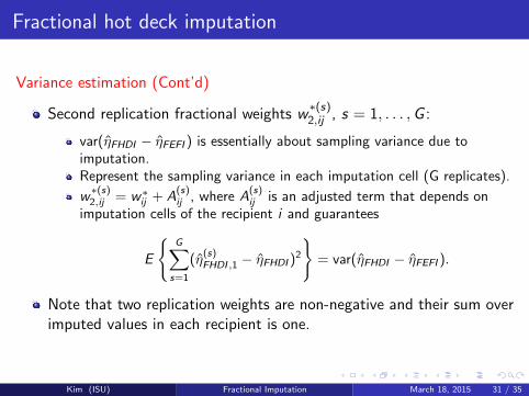
Variance estimation (Cont’d)
Second replication fractional weights w∗(s)2,ij , s = 1, . . . ,G :
var(η̂FHDI − η̂FEFI ) is essentially about sampling variance due toimputation.Represent the sampling variance in each imputation cell (G replicates).
w∗(s)2,ij = w∗ij + A
(s)ij , where A
(s)ij is an adjusted term that depends on
imputation cells of the recipient i and guarantees
E
{G∑
s=1
(η̂(s)FHDI ,1 − η̂FHDI )
2
}= var(η̂FHDI − η̂FEFI ).
Note that two replication weights are non-negative and their sum overimputed values in each recipient is one.
Kim (ISU) Fractional Imputation March 18, 2015 31 / 35
Fractional hot deck imputation
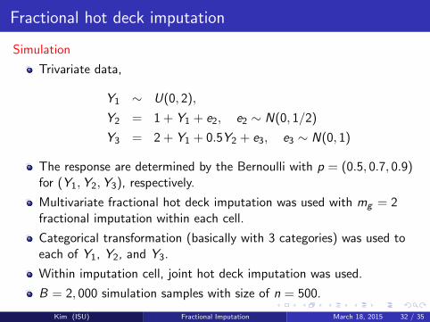
Simulation
Trivariate data,
Y1 ∼ U(0, 2),
Y2 = 1 + Y1 + e2, e2 ∼ N(0, 1/2)
Y3 = 2 + Y1 + 0.5Y2 + e3, e3 ∼ N(0, 1)
The response are determined by the Bernoulli with p = (0.5, 0.7, 0.9)for (Y1,Y2,Y3), respectively.
Multivariate fractional hot deck imputation was used with mg = 2fractional imputation within each cell.
Categorical transformation (basically with 3 categories) was used toeach of Y1, Y2, and Y3.
Within imputation cell, joint hot deck imputation was used.
B = 2, 000 simulation samples with size of n = 500.
Kim (ISU) Fractional Imputation March 18, 2015 32 / 35
Fractional hot deck imputation
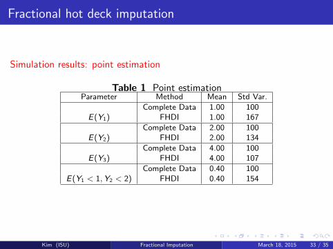
Simulation results: point estimation
Table 1 Point estimationParameter Method Mean Std Var.
Complete Data 1.00 100E(Y1) FHDI 1.00 167
Complete Data 2.00 100E(Y2) FHDI 2.00 134
Complete Data 4.00 100E(Y3) FHDI 4.00 107
Complete Data 0.40 100E(Y1 < 1,Y2 < 2) FHDI 0.40 154
Kim (ISU) Fractional Imputation March 18, 2015 33 / 35
Fractional hot deck imputation
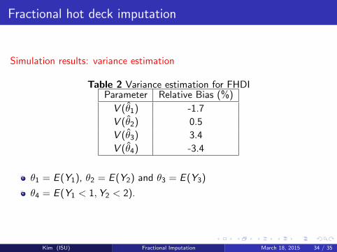
Simulation results: variance estimation
Table 2 Variance estimation for FHDIParameter Relative Bias (%)
V (θ̂1) -1.7
V (θ̂2) 0.5
V (θ̂3) 3.4
V (θ̂4) -3.4
θ1 = E (Y1), θ2 = E (Y2) and θ3 = E (Y3)
θ4 = E (Y1 < 1,Y2 < 2).
Kim (ISU) Fractional Imputation March 18, 2015 34 / 35
Conclusion
Fractional hot deck imputation is considered.
Categorical data transformation was used for approximation.
Does not rely on parametric model assumptions.Two-step imputation
1 Step 1: Allocation of Imputation of cells2 Step 2: Joint hot deck imputation within imputation cell.
Replication-based approach for imputation variance estimation.
To be implemented in SAS: Proc SurveyImpute
Kim (ISU) Fractional Imputation March 18, 2015 35 / 35