Fourth Order Exponential Time Integrators for the …berland/talks/berland04magic.pdfFourth Order...
47
Fourth Order Exponential Time Integrators for the Nonlinear Schrödinger Equation MaGIC Workshop 2004, Røros Håvard Berland, joint work with Bård Skaflestad and Brynjulf Owren NTNU Fourth Order Exponential Time Integrators for the Nonlinear Schrödinger Equation – p.1/24
Transcript of Fourth Order Exponential Time Integrators for the …berland/talks/berland04magic.pdfFourth Order...
Fourth Order Exponential TimeIntegrators for the Nonlinear
Schrödinger EquationMaGIC Workshop 2004, Røros
Håvard Berland, joint work with Bård Skaflestad and Brynjulf Owren
NTNU
Fourth Order Exponential Time Integrators for the Nonlinear Schrödinger Equation – p.1/24
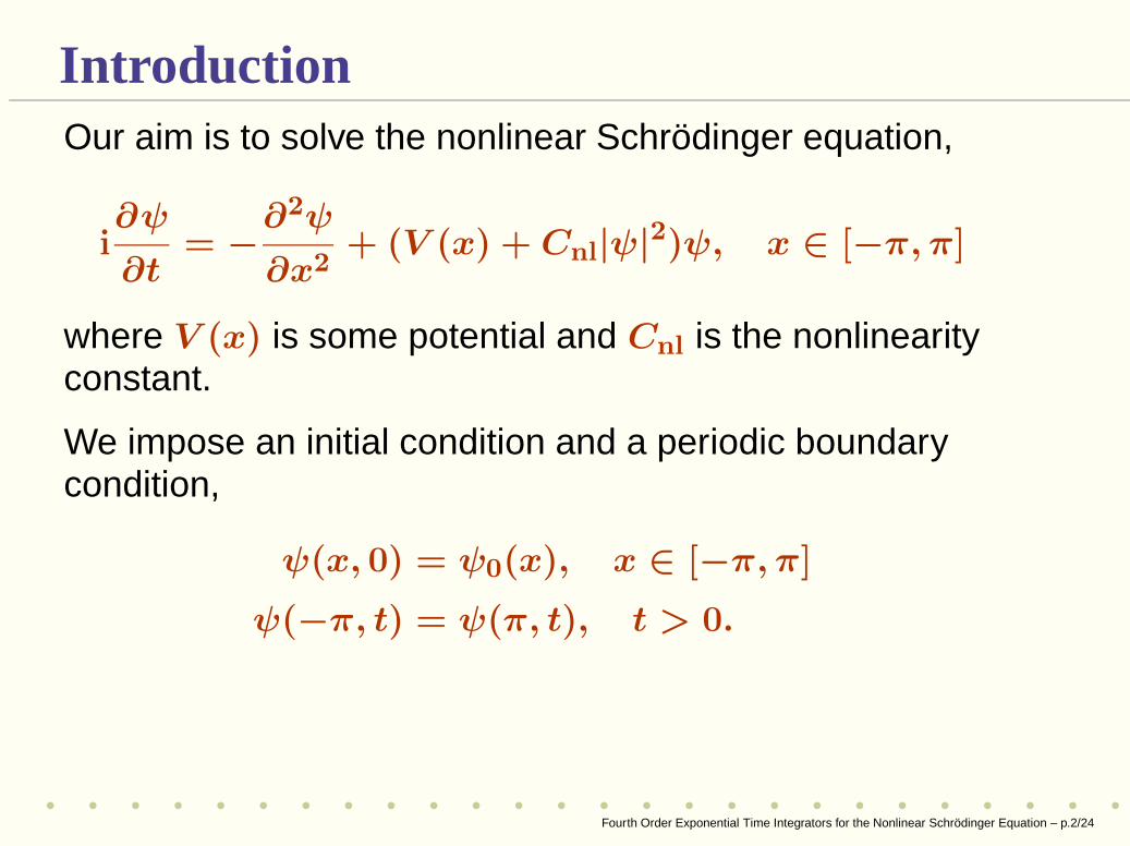
IntroductionOur aim is to solve the nonlinear Schrödinger equation,
i∂ψ
∂t= −
∂2ψ
∂x2+ (V (x) + Cnl|ψ|2)ψ, x ∈ [−π, π]
where V (x) is some potential and Cnl is the nonlinearityconstant.
We impose an initial condition and a periodic boundarycondition,
ψ(x, 0) = ψ0(x), x ∈ [−π, π]
ψ(−π, t) = ψ(π, t), t > 0.
Fourth Order Exponential Time Integrators for the Nonlinear Schrödinger Equation – p.2/24
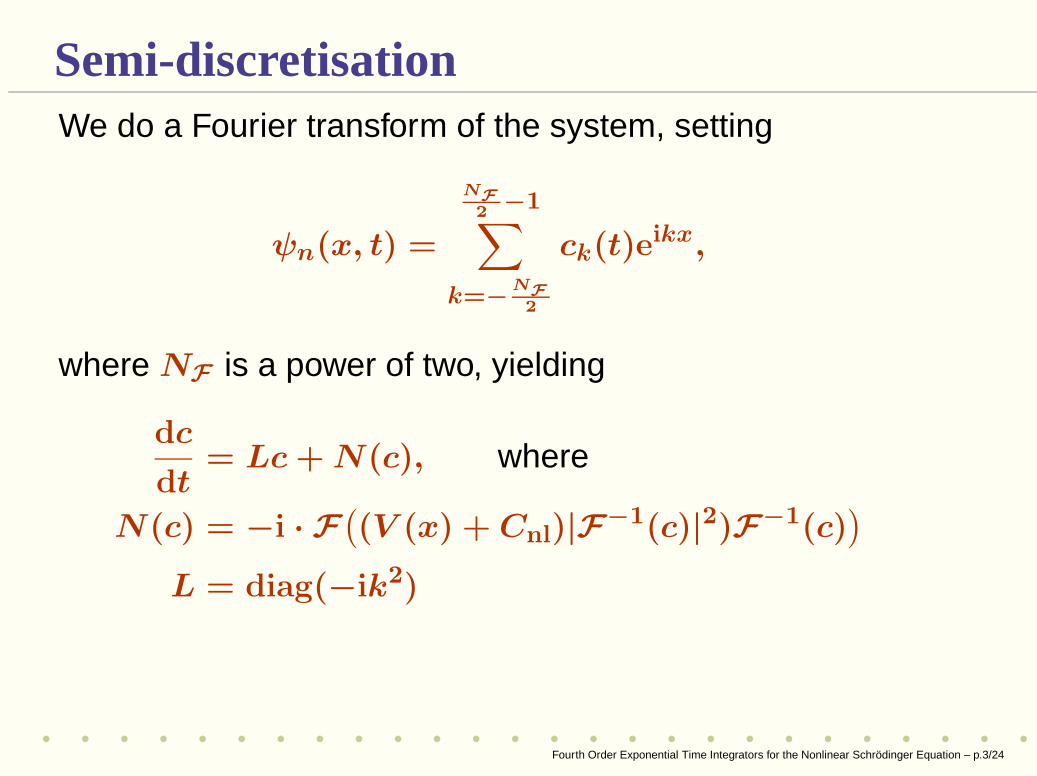
Semi-discretisationWe do a Fourier transform of the system, setting
ψn(x, t) =
NF2
−1∑
k=−NF2
ck(t)eikx,
where NF is a power of two, yielding
dc
dt= Lc+N(c), where
N(c) = −i · F(
(V (x) + Cnl)|F−1(c)|2)F−1(c)
)
L = diag(−ik2)
Fourth Order Exponential Time Integrators for the Nonlinear Schrödinger Equation – p.3/24
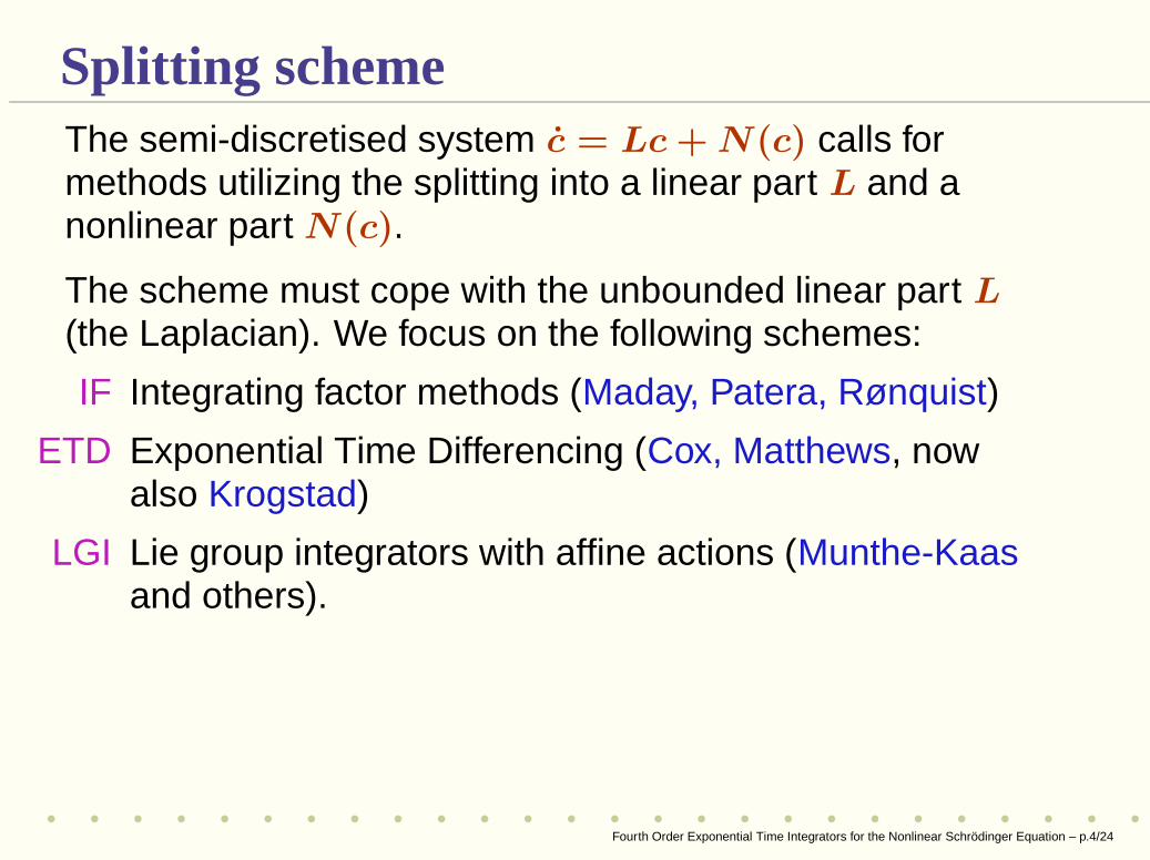
Splitting schemeThe semi-discretised system c = Lc+N(c) calls formethods utilizing the splitting into a linear part L and anonlinear part N(c).
The scheme must cope with the unbounded linear part L(the Laplacian). We focus on the following schemes:
IF Integrating factor methods (Maday, Patera, Rønquist)
ETD Exponential Time Differencing (Cox, Matthews, nowalso Krogstad)
LGI Lie group integrators with affine actions (Munthe-Kaasand others).
Fourth Order Exponential Time Integrators for the Nonlinear Schrödinger Equation – p.4/24
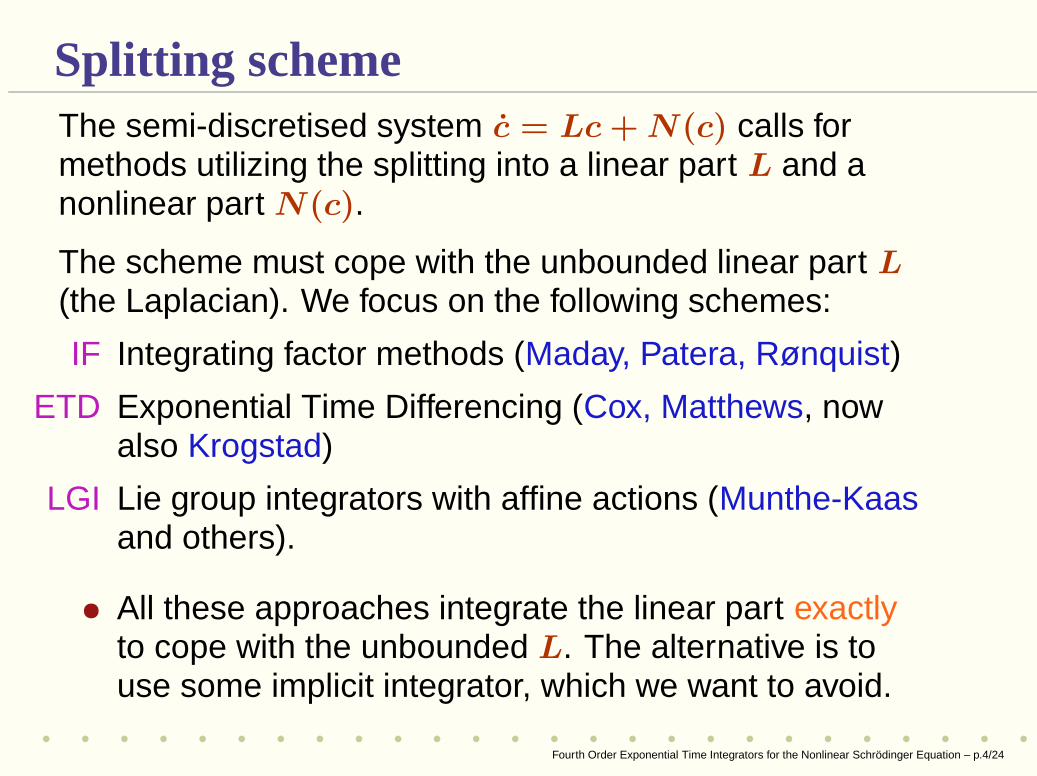
Splitting schemeThe semi-discretised system c = Lc+N(c) calls formethods utilizing the splitting into a linear part L and anonlinear part N(c).
The scheme must cope with the unbounded linear part L(the Laplacian). We focus on the following schemes:
IF Integrating factor methods (Maday, Patera, Rønquist)
ETD Exponential Time Differencing (Cox, Matthews, nowalso Krogstad)
LGI Lie group integrators with affine actions (Munthe-Kaasand others).
• All these approaches integrate the linear part exactlyto cope with the unbounded L. The alternative is touse some implicit integrator, which we want to avoid.
Fourth Order Exponential Time Integrators for the Nonlinear Schrödinger Equation – p.4/24
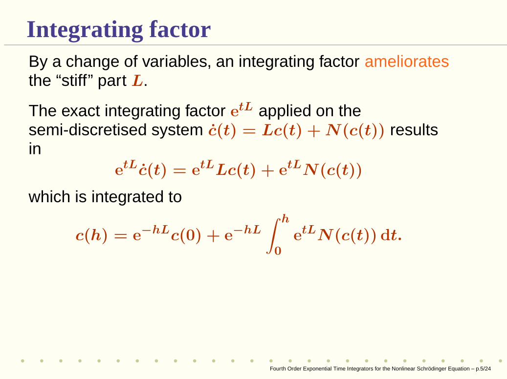
Integrating factorBy a change of variables, an integrating factor amelioratesthe “stiff” part L.
The exact integrating factor etL applied on thesemi-discretised system c(t) = Lc(t) +N(c(t)) resultsin
etLc(t) = etLLc(t) + etLN(c(t))
which is integrated to
c(h) = e−hLc(0) + e−hL
∫ h
0etLN(c(t)) dt.
• Our methods OIFS, ETD and LGI can all be thoughtof as arising from different ways of evaluating theintegral above.
Fourth Order Exponential Time Integrators for the Nonlinear Schrödinger Equation – p.5/24
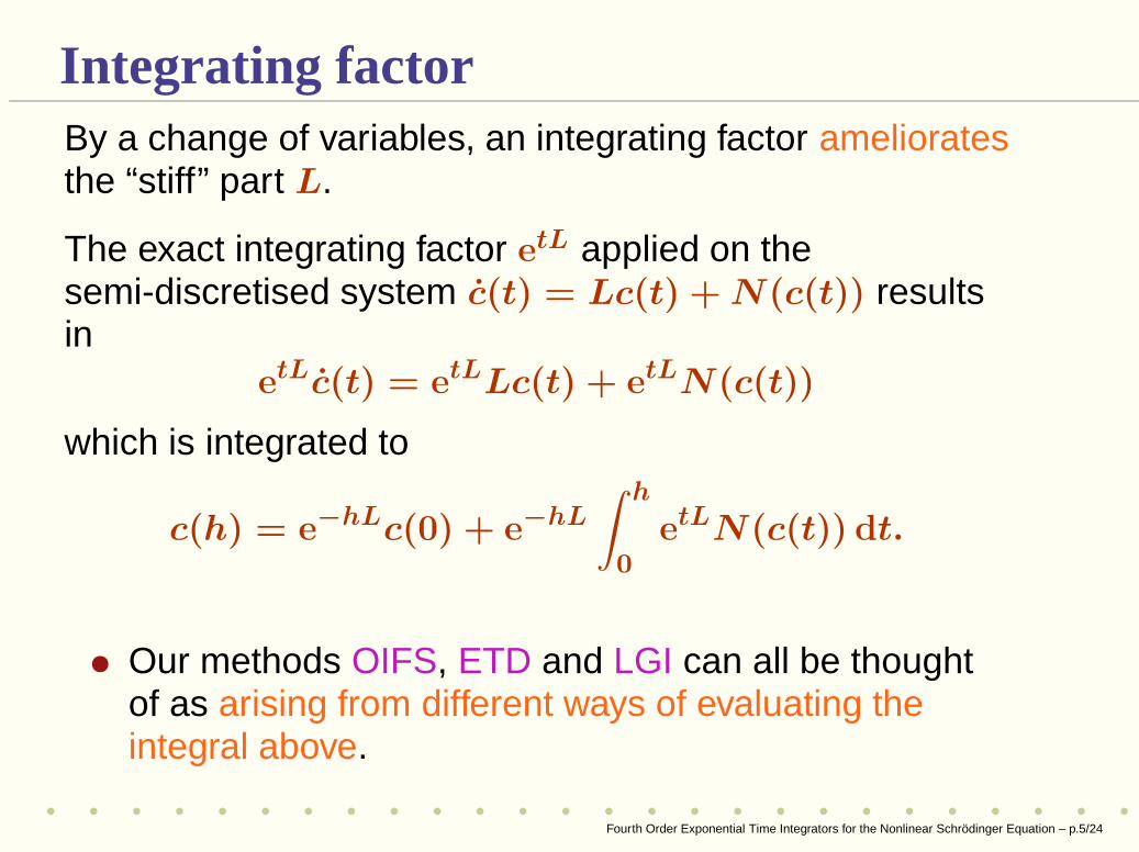
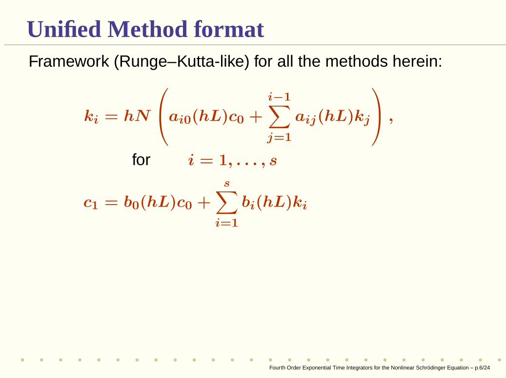
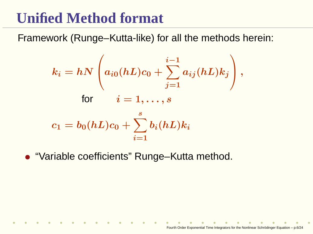
Unified Method formatFramework (Runge–Kutta-like) for all the methods herein:
ki = hN
ai0(hL)c0 +
i−1∑
j=1
aij(hL)kj
,
for i = 1, . . . , s
c1 = b0(hL)c0 +
s∑
i=1
bi(hL)ki
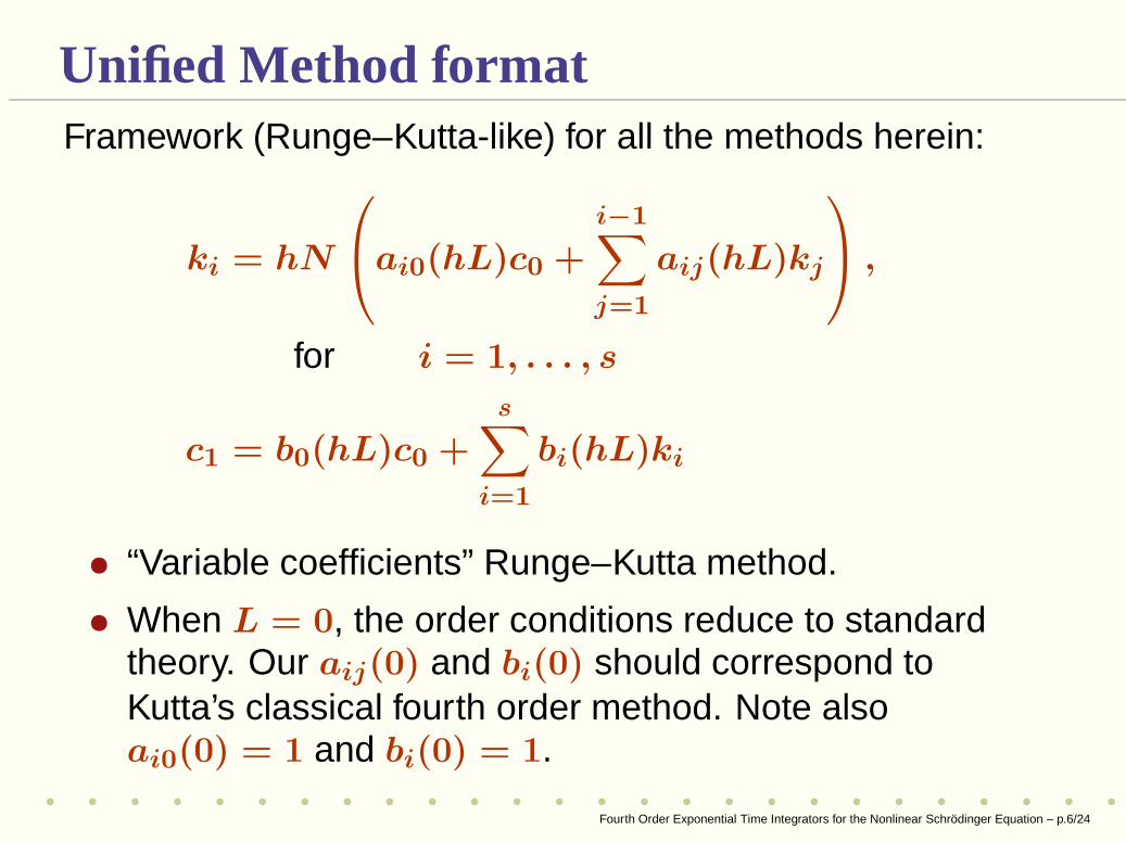
• “Variable coefficients” Runge–Kutta method.
• When L = 0, the order conditions reduce to standardtheory. Our aij(0) and bi(0) should correspond toKutta’s classical fourth order method. Note alsoai0(0) = 1 and bi(0) = 1.
Fourth Order Exponential Time Integrators for the Nonlinear Schrödinger Equation – p.6/24
Unified Method formatFramework (Runge–Kutta-like) for all the methods herein:
ki = hN
ai0(hL)c0 +
i−1∑
j=1
aij(hL)kj
,
for i = 1, . . . , s
c1 = b0(hL)c0 +
s∑
i=1
bi(hL)ki
• “Variable coefficients” Runge–Kutta method.
• When L = 0, the order conditions reduce to standardtheory. Our aij(0) and bi(0) should correspond toKutta’s classical fourth order method. Note alsoai0(0) = 1 and bi(0) = 1.
Fourth Order Exponential Time Integrators for the Nonlinear Schrödinger Equation – p.6/24
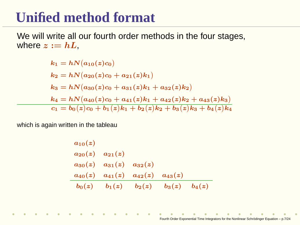
Unified method formatWe will write all our fourth order methods in the four stages,where z := hL,
k1 = hN`
a10(z)c0´
k2 = hN`
a20(z)c0 + a21(z)k1´
k3 = hN`
a30(z)c0 + a31(z)k1 + a32(z)k2´
k4 = hN`
a40(z)c0 + a41(z)k1 + a42(z)k2 + a43(z)k3´
c1 = b0`
z´
c0 + b1`
z´
k1 + b2`
z´
k2 + b3`
z´
k3 + b4`
z´
k4
which is again written in the tableau
a10(z)
a20(z) a21(z)
a30(z) a31(z) a32(z)
a40(z) a41(z) a42(z) a43(z)
b0(z) b1(z) b2(z) b3(z) b4(z)
Fourth Order Exponential Time Integrators for the Nonlinear Schrödinger Equation – p.7/24
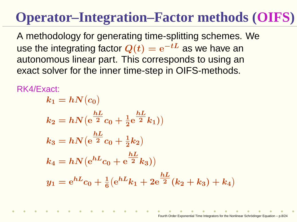
Operator–Integration–Factor methods (OIFS)A methodology for generating time-splitting schemes. Weuse the integrating factor Q(t) = e−tL as we have anautonomous linear part. This corresponds to using anexact solver for the inner time-step in OIFS-methods.
RK4/Exact:k1 = hN
(
c0)
k2 = hN(
ehL2 c0 + 1
2e
hL2 k1)
)
k3 = hN(
ehL2 c0 + 1
2k2
)
k4 = hN(
ehLc0 + ehL2 k3)
)
y1 = ehLc0 + 16
(
ehLk1 + 2ehL2 (k2 + k3) + k4
)
Fourth Order Exponential Time Integrators for the Nonlinear Schrödinger Equation – p.8/24
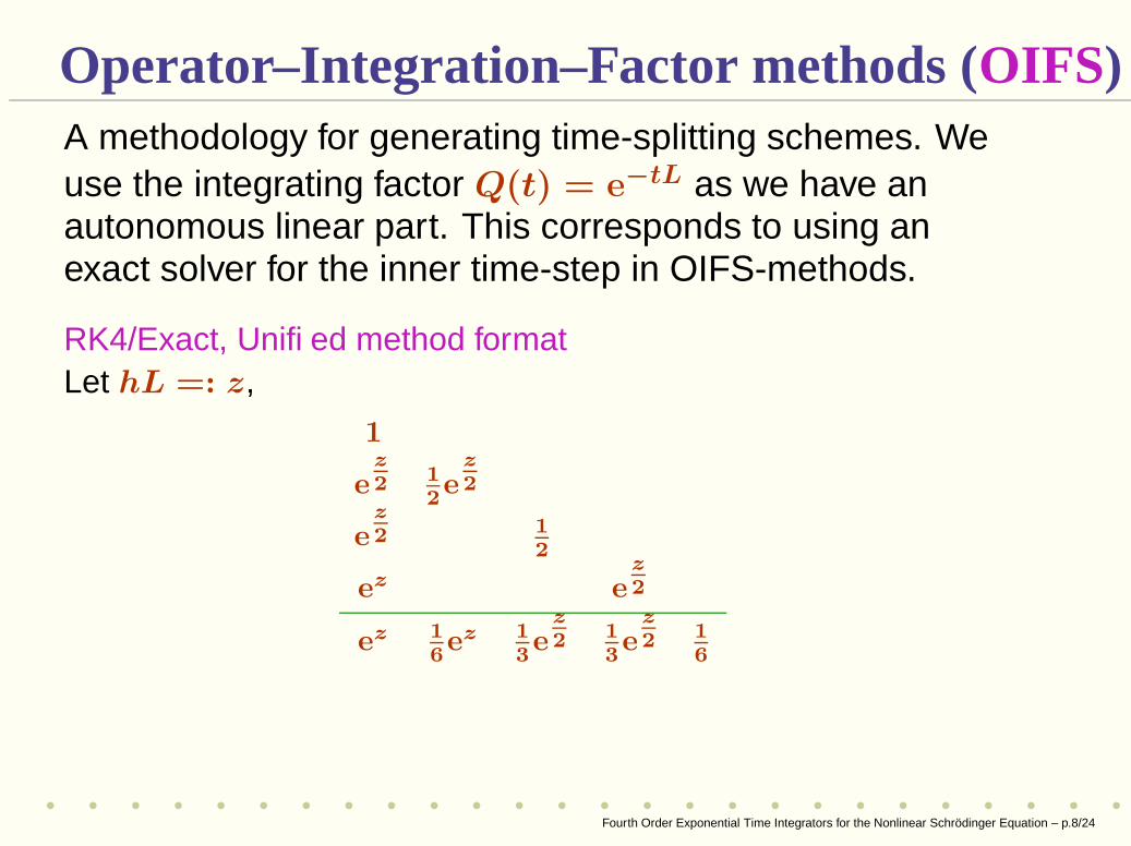
Operator–Integration–Factor methods (OIFS)A methodology for generating time-splitting schemes. Weuse the integrating factor Q(t) = e−tL as we have anautonomous linear part. This corresponds to using anexact solver for the inner time-step in OIFS-methods.
RK4/Exact, Unified method formatLet hL =: z,
1
ez2 1
2e
z2
ez2 1
2
ez ez2
ez 16ez 1
3e
z2 1
3e
z2 1
6
Fourth Order Exponential Time Integrators for the Nonlinear Schrödinger Equation – p.8/24
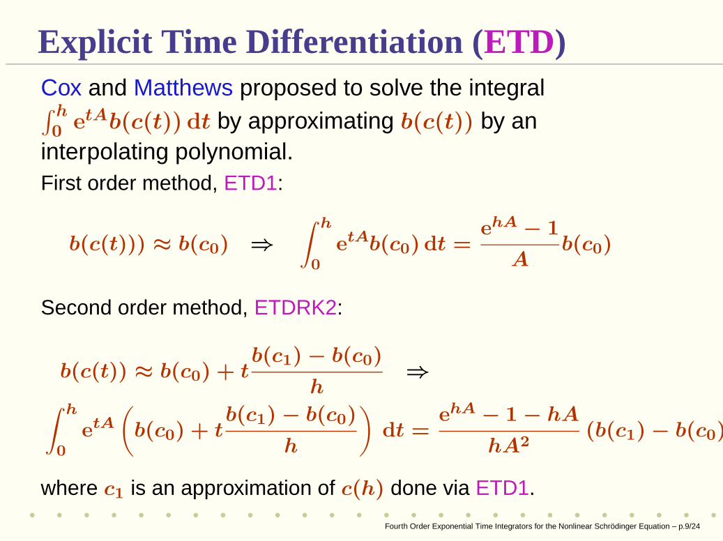
Explicit Time Differentiation (ETD)Cox and Matthews proposed to solve the integral∫ h0 etAb(c(t)) dt by approximating b(c(t)) by an
interpolating polynomial.First order method, ETD1:
b(c(t))) ≈ b(c0) ⇒
∫ h
0etAb(c0) dt =
ehA − 1
Ab(c0)
Second order method, ETDRK2:
b(c(t)) ≈ b(c0) + tb(c1) − b(c0)
h⇒
∫ h
0etA
(
b(c0) + tb(c1) − b(c0)
h
)
dt =ehA − 1 − hA
hA2(b(c1) − b(c0))
where c1 is an approximation of c(h) done via ETD1.
Fourth Order Exponential Time Integrators for the Nonlinear Schrödinger Equation – p.9/24
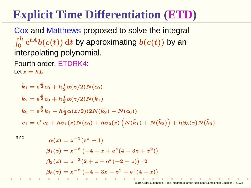
Explicit Time Differentiation (ETD)Cox and Matthews proposed to solve the integral∫ h0 etAb(c(t)) dt by approximating b(c(t)) by an
interpolating polynomial.Fourth order, ETDRK4:Let z = hL,
k1 = ez2 c0 + h1
2α(z/2)N(c0)
k2 = ez2 c0 + h1
2α(z/2)N(k1)
k3 = ez2 k1 + h1
2α(z/2)(2N(k2) − N(c0))
c1 = ezc0 + hβ1(z)N(c0) + hβ2(z)“
N(k1) + N(k2)”
+ hβ3(z)N(k3)
andα(z) = z−1
`
ez − 1´
β1(z) = z−3`
−4 − z + ez(4 − 3z + z2)´
β2(z) = z−3`
2 + z + ez(−2 + z)´
· 2
β3(z) = z−3`
−4 − 3z − z2 + ez(4 − z)´
Fourth Order Exponential Time Integrators for the Nonlinear Schrödinger Equation – p.9/24
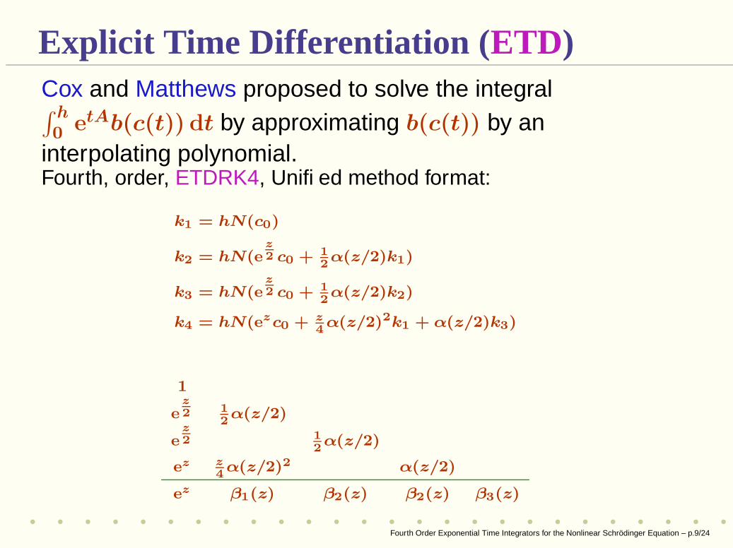
Explicit Time Differentiation (ETD)Cox and Matthews proposed to solve the integral∫ h0 etAb(c(t)) dt by approximating b(c(t)) by an
interpolating polynomial.Fourth, order, ETDRK4, Unified method format:
k1 = hN(c0)
k2 = hN(ez2 c0 + 1
2α(z/2)k1)
k3 = hN(ez2 c0 + 1
2α(z/2)k2)
k4 = hN(ezc0 + z4
α(z/2)2k1 + α(z/2)k3)
1
ez2 1
2α(z/2)
ez2 1
2α(z/2)
ez z4
α(z/2)2 α(z/2)
ez β1(z) β2(z) β2(z) β3(z)
Fourth Order Exponential Time Integrators for the Nonlinear Schrödinger Equation – p.9/24
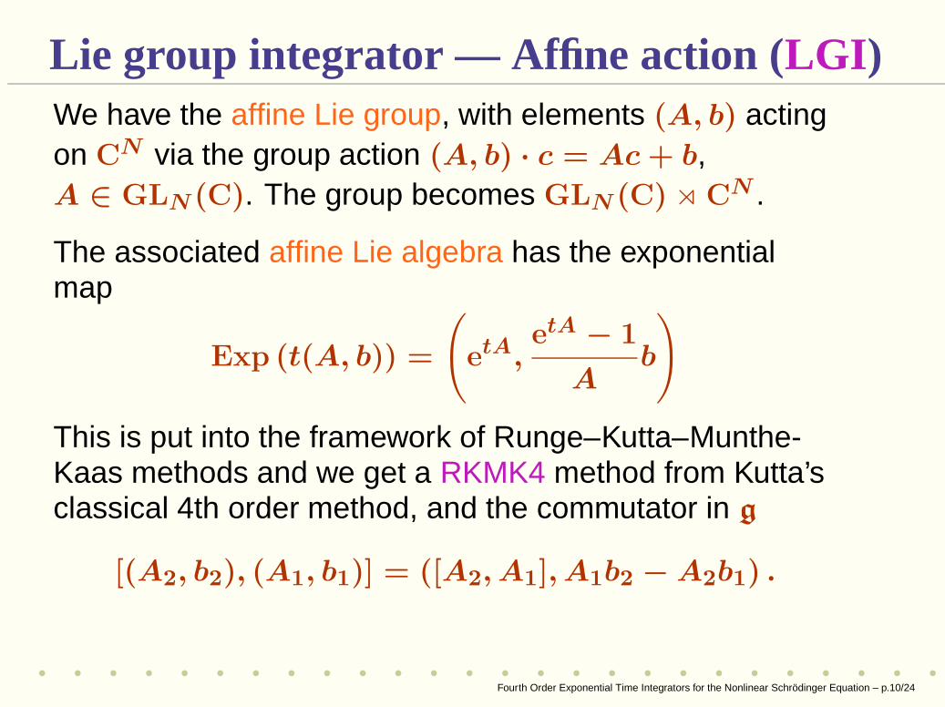
Lie group integrator — Affine action (LGI)We have the affine Lie group, with elements (A, b) actingon CN via the group action (A, b) · c = Ac+ b,A ∈ GLN(C). The group becomes GLN(C) o CN .
The associated affine Lie algebra has the exponentialmap
Exp (t(A, b)) =
(
etA,etA − 1
Ab
)
This is put into the framework of Runge–Kutta–Munthe-Kaas methods and we get a RKMK4 method from Kutta’sclassical 4th order method, and the commutator in g
[(A2, b2), (A1, b1)] = ([A2, A1], A1b2 −A2b1) .
Fourth Order Exponential Time Integrators for the Nonlinear Schrödinger Equation – p.10/24
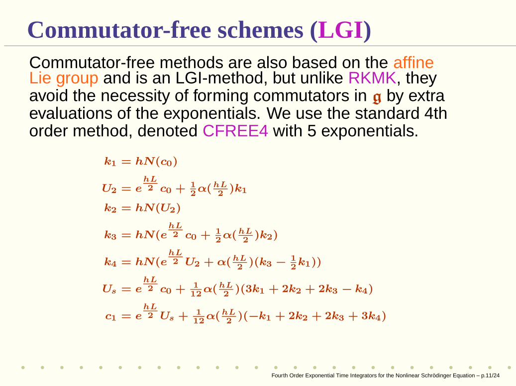
Commutator-free schemes (LGI)Commutator-free methods are also based on the affineLie group and is an LGI-method, but unlike RKMK, theyavoid the necessity of forming commutators in g by extraevaluations of the exponentials. We use the standard 4thorder method, denoted CFREE4 with 5 exponentials.
k1 = hN(c0)
U2 = ehL2 c0 + 1
2α(hL
2)k1
k2 = hN(U2)
k3 = hN(ehL2 c0 + 1
2α(hL
2)k2)
k4 = hN(ehL2 U2 + α(hL
2)(k3 − 1
2k1))
Us = ehL2 c0 + 1
12α(hL
2)(3k1 + 2k2 + 2k3 − k4)
c1 = ehL2 Us + 1
12α(hL
2)(−k1 + 2k2 + 2k3 + 3k4)
Fourth Order Exponential Time Integrators for the Nonlinear Schrödinger Equation – p.11/24
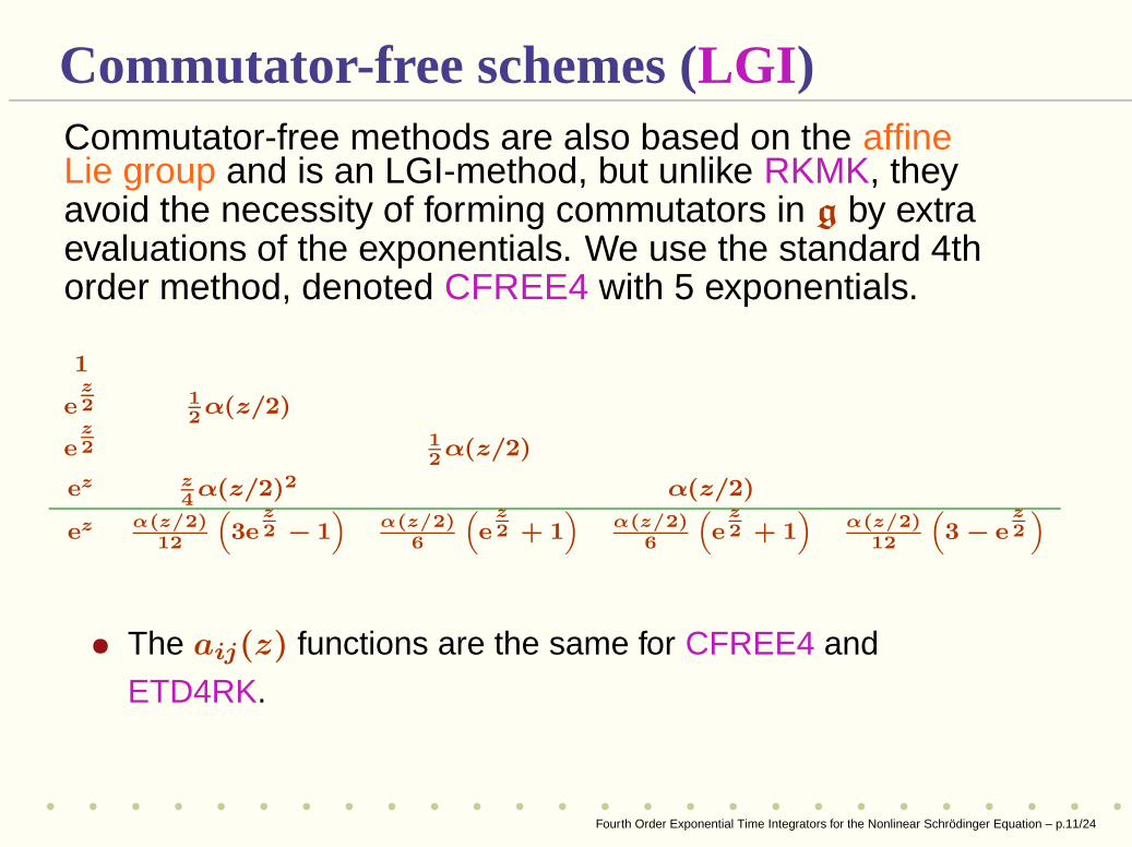
Commutator-free schemes (LGI)Commutator-free methods are also based on the affineLie group and is an LGI-method, but unlike RKMK, theyavoid the necessity of forming commutators in g by extraevaluations of the exponentials. We use the standard 4thorder method, denoted CFREE4 with 5 exponentials.
1
ez2 1
2α(z/2)
ez2 1
2α(z/2)
ez z4
α(z/2)2 α(z/2)
ez α(z/2)12
“
3ez2 − 1
”
α(z/2)6
“
ez2 + 1
”
α(z/2)6
“
ez2 + 1
”
α(z/2)12
“
3 − ez2
”
• The aij(z) functions are the same for CFREE4 and
ETD4RK.
Fourth Order Exponential Time Integrators for the Nonlinear Schrödinger Equation – p.11/24
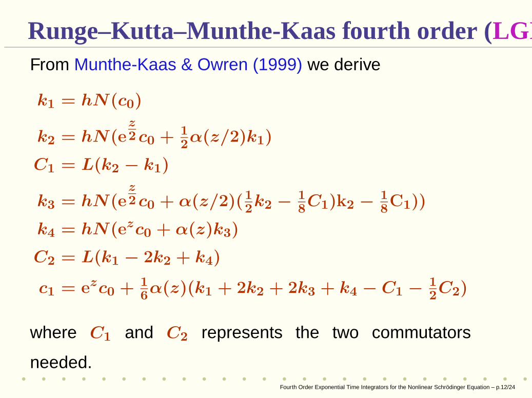
Runge–Kutta–Munthe-Kaas fourth order (LGI)From Munthe-Kaas & Owren (1999) we derive
k1 = hN(c0)
k2 = hN(ez2c0 + 1
2α(z/2)k1)
C1 = L(k2 − k1)
k3 = hN(ez2c0 + α(z/2)(1
2k2 − 1
8C1)k2 − 1
8C1))
k4 = hN(ezc0 + α(z)k3)
C2 = L(k1 − 2k2 + k4)
c1 = ezc0 + 16α(z)(k1 + 2k2 + 2k3 + k4 − C1 − 1
2C2)
where C1 and C2 represents the two commutators
needed.Fourth Order Exponential Time Integrators for the Nonlinear Schrödinger Equation – p.12/24
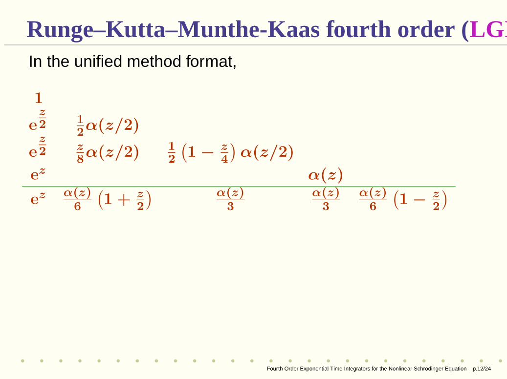
Runge–Kutta–Munthe-Kaas fourth order (LGI)In the unified method format,
1
ez2 1
2α(z/2)
ez2 z
8α(z/2) 12
(
1 − z4
)
α(z/2)
ez α(z)
ez α(z)6
(
1 + z2
) α(z)3
α(z)3
α(z)6
(
1 − z2
)
Fourth Order Exponential Time Integrators for the Nonlinear Schrödinger Equation – p.12/24
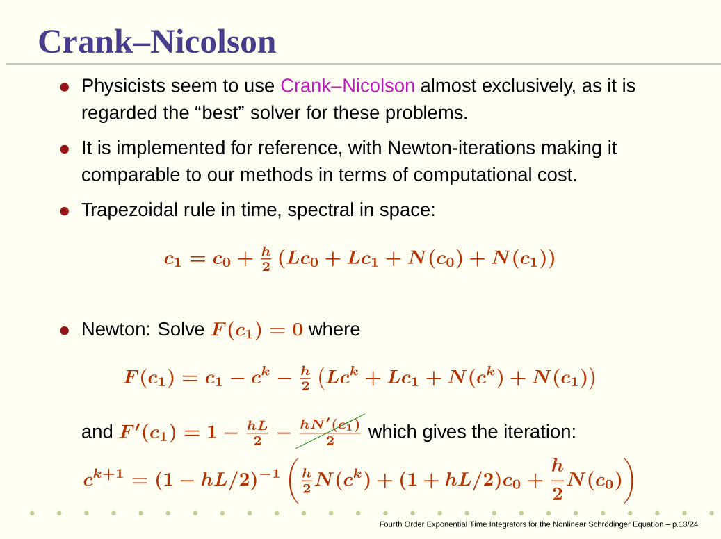
Crank–Nicolson• Physicists seem to use Crank–Nicolson almost exclusively, as it is
regarded the “best” solver for these problems.
• It is implemented for reference, with Newton-iterations making itcomparable to our methods in terms of computational cost.
• Trapezoidal rule in time, spectral in space:
c1 = c0 + h2
(Lc0 + Lc1 +N(c0) +N(c1))
• Newton: Solve F (c1) = 0 where
F (c1) = c1 − ck − h2
(
Lck + Lc1 +N(ck) +N(c1))
and F ′(c1) = 1 − hL2
−�
���hN ′(c1)
2which gives the iteration:
ck+1 = (1 − hL/2)−1
(
h2N(ck) + (1 + hL/2)c0 +
h
2N(c0)
)
Fourth Order Exponential Time Integrators for the Nonlinear Schrödinger Equation – p.13/24
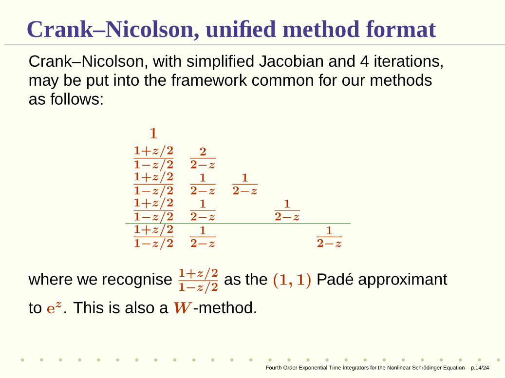
Crank–Nicolson, unified method formatCrank–Nicolson, with simplified Jacobian and 4 iterations,may be put into the framework common for our methodsas follows:
11+z/21−z/2
22−z
1+z/21−z/2
12−z
12−z
1+z/21−z/2
12−z
12−z
1+z/21−z/2
12−z
12−z
where we recognise 1+z/21−z/2
as the (1, 1) Padé approximant
to ez. This is also a W -method.
Fourth Order Exponential Time Integrators for the Nonlinear Schrödinger Equation – p.14/24
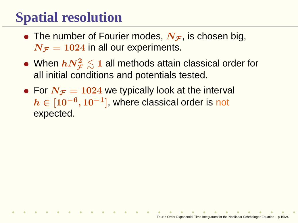
Spatial resolution• The number of Fourier modes, NF , is chosen big,NF = 1024 in all our experiments.
• When hN2F . 1 all methods attain classical order for
all initial conditions and potentials tested.
• For NF = 1024 we typically look at the intervalh ∈ [10−6, 10−1], where classical order is notexpected.
Fourth Order Exponential Time Integrators for the Nonlinear Schrödinger Equation – p.15/24
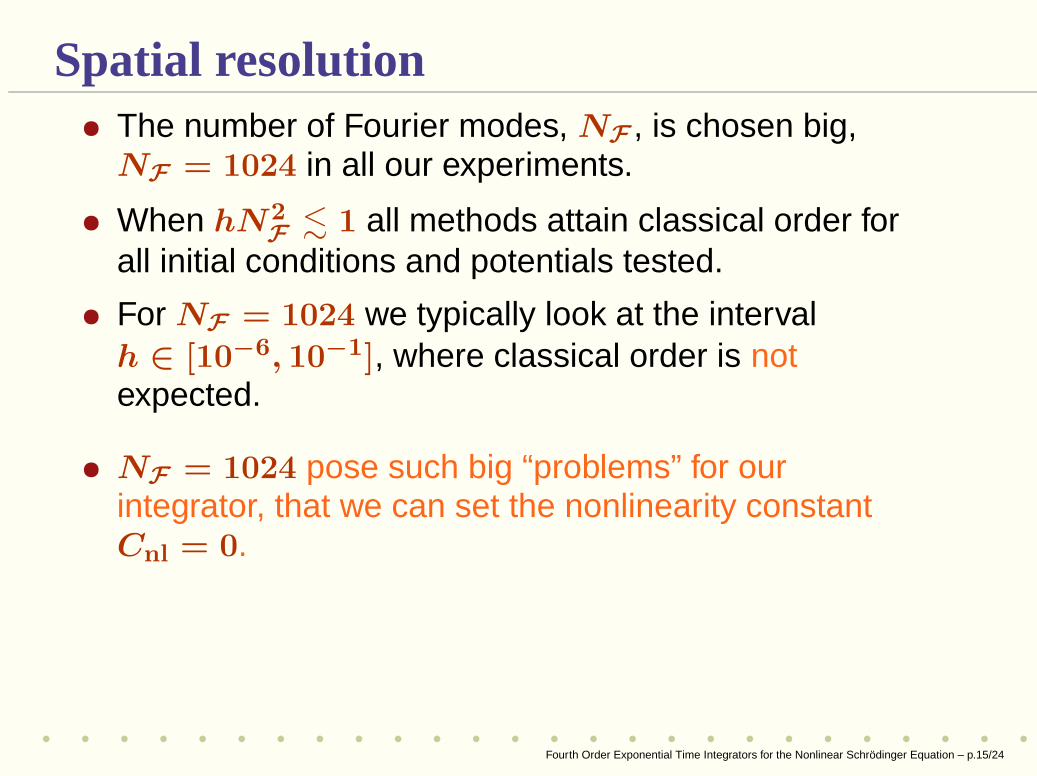
Spatial resolution• The number of Fourier modes, NF , is chosen big,NF = 1024 in all our experiments.
• When hN2F . 1 all methods attain classical order for
all initial conditions and potentials tested.
• For NF = 1024 we typically look at the intervalh ∈ [10−6, 10−1], where classical order is notexpected.
• NF = 1024 pose such big “problems” for ourintegrator, that we can set the nonlinearity constantCnl = 0.
Fourth Order Exponential Time Integrators for the Nonlinear Schrödinger Equation – p.15/24
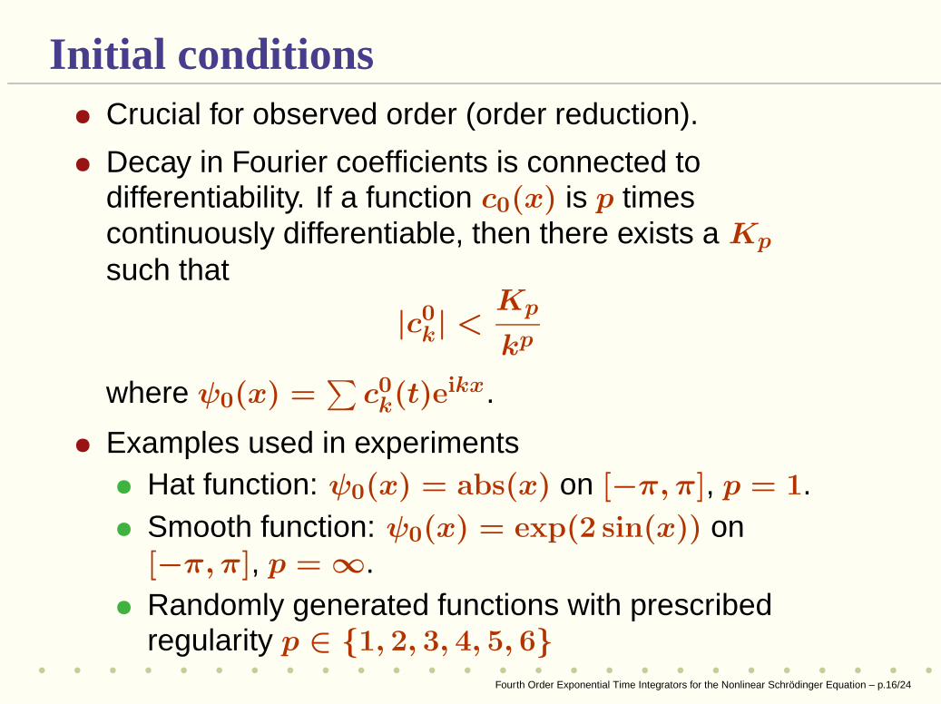
Initial conditions• Crucial for observed order (order reduction).
• Decay in Fourier coefficients is connected todifferentiability. If a function c0(x) is p timescontinuously differentiable, then there exists a Kp
such that
|c0k| <Kp
kp
where ψ0(x) =∑
c0k(t)eikx.
• Examples used in experiments• Hat function: ψ0(x) = abs(x) on [−π, π], p = 1.• Smooth function: ψ0(x) = exp(2 sin(x)) on
[−π, π], p = ∞.• Randomly generated functions with prescribed
regularity p ∈ {1, 2, 3, 4, 5, 6}
Fourth Order Exponential Time Integrators for the Nonlinear Schrödinger Equation – p.16/24
PotentialsVarious potensials V (x) have been used.
• Smooth potential
• Hat potential
• Random potential with prescribed regularity
• Constant potential, V (x) ≡ λ. The system ofequations decouples.
We will see that a potential with low regularity also leads to
order reduction.
Fourth Order Exponential Time Integrators for the Nonlinear Schrödinger Equation – p.17/24
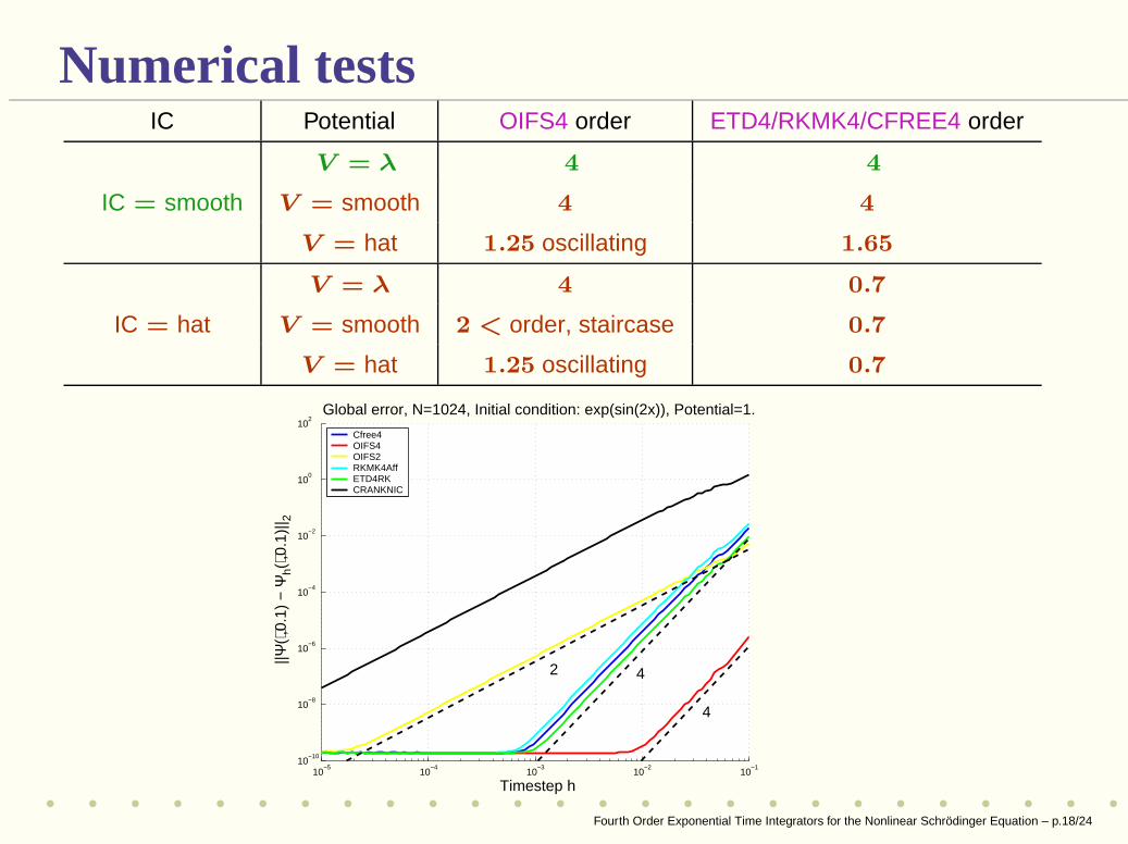
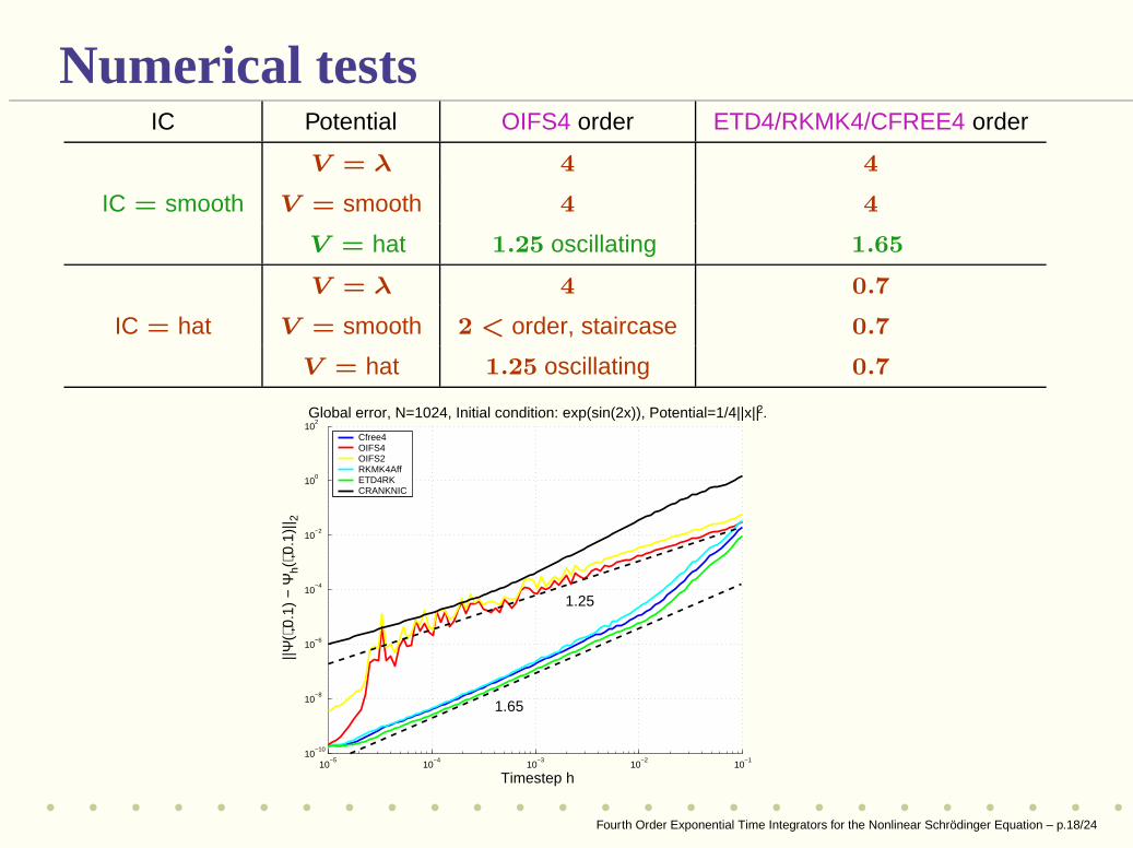
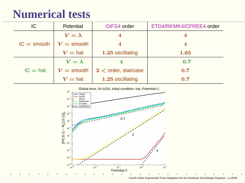
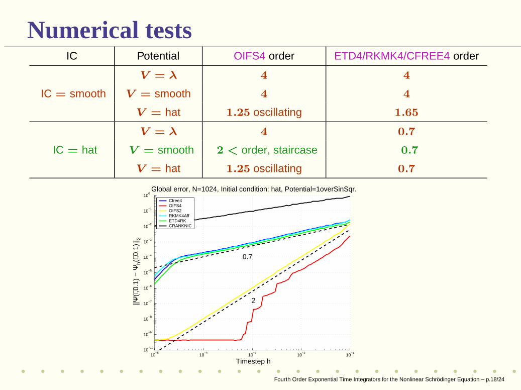
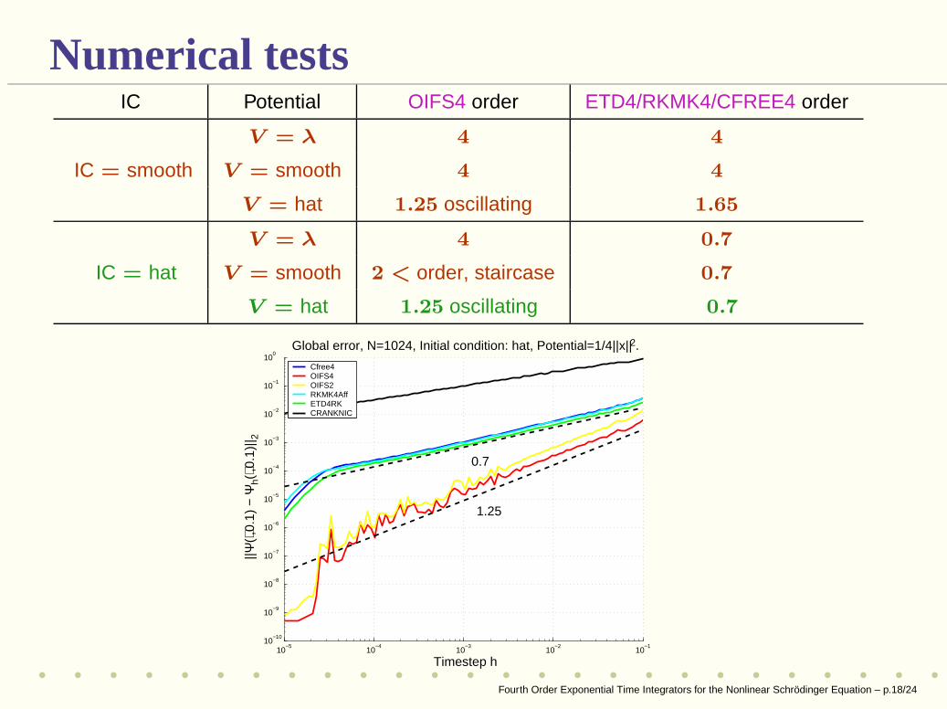
Numerical testsIC Potential OIFS4 order ETD4/RKMK4/CFREE4 order
V = λ 4 4
IC = smooth V = smooth 4 4
V = hat 1.25 oscillating 1.65
V = λ 4 0.7
IC = hat V = smooth 2 < order, staircase 0.7
V = hat 1.25 oscillating 0.7
10−5
10−4
10−3
10−2
10−1
10−10
10−8
10−6
10−4
10−2
100
102
Timestep h
||Ψ
(⋅,0.
1) −
Ψh(
⋅,0.1
)|| 2
Global error, N=1024, Initial condition: exp(sin(2x)), Potential=1.
4
42
Cfree4OIFS4OIFS2RKMK4AffETD4RKCRANKNIC
Fourth Order Exponential Time Integrators for the Nonlinear Schrödinger Equation – p.18/24
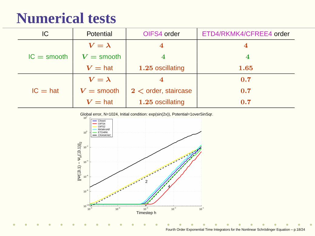
Numerical testsIC Potential OIFS4 order ETD4/RKMK4/CFREE4 order
V = λ 4 4
IC = smooth V = smooth 4 4
V = hat 1.25 oscillating 1.65
V = λ 4 0.7
IC = hat V = smooth 2 < order, staircase 0.7
V = hat 1.25 oscillating 0.7
10−5
10−4
10−3
10−2
10−1
10−10
10−8
10−6
10−4
10−2
100
102
Timestep h
||Ψ
(⋅,0.
1) −
Ψh(
⋅,0.1
)|| 2
Global error, N=1024, Initial condition: exp(sin(2x)), Potential=1overSinSqr.
42
Cfree4OIFS4OIFS2RKMK4AffETD4RKCRANKNIC
Fourth Order Exponential Time Integrators for the Nonlinear Schrödinger Equation – p.18/24
Numerical testsIC Potential OIFS4 order ETD4/RKMK4/CFREE4 order
V = λ 4 4
IC = smooth V = smooth 4 4
V = hat 1.25 oscillating 1.65
V = λ 4 0.7
IC = hat V = smooth 2 < order, staircase 0.7
V = hat 1.25 oscillating 0.7
10−5
10−4
10−3
10−2
10−1
10−10
10−8
10−6
10−4
10−2
100
102
Timestep h
||Ψ
(⋅,0.
1) −
Ψh(
⋅,0.1
)|| 2
Global error, N=1024, Initial condition: exp(sin(2x)), Potential=1/4||x||2.
1.65
1.25
Cfree4OIFS4OIFS2RKMK4AffETD4RKCRANKNIC
Fourth Order Exponential Time Integrators for the Nonlinear Schrödinger Equation – p.18/24
Numerical testsIC Potential OIFS4 order ETD4/RKMK4/CFREE4 order
V = λ 4 4
IC = smooth V = smooth 4 4
V = hat 1.25 oscillating 1.65
V = λ 4 0.7
IC = hat V = smooth 2 < order, staircase 0.7
V = hat 1.25 oscillating 0.7
10−5
10−4
10−3
10−2
10−1
10−10
10−9
10−8
10−7
10−6
10−5
10−4
10−3
10−2
10−1
100
Timestep h
||Ψ
(⋅,0.
1) −
Ψh(
⋅,0.1
)|| 2
Global error, N=1024, Initial condition: hat, Potential=1.
4
2
0.7
Cfree4OIFS4OIFS2RKMK4AffETD4RKCRANKNIC
Fourth Order Exponential Time Integrators for the Nonlinear Schrödinger Equation – p.18/24
Numerical testsIC Potential OIFS4 order ETD4/RKMK4/CFREE4 order
V = λ 4 4
IC = smooth V = smooth 4 4
V = hat 1.25 oscillating 1.65
V = λ 4 0.7
IC = hat V = smooth 2 < order, staircase 0.7
V = hat 1.25 oscillating 0.7
10−5
10−4
10−3
10−2
10−1
10−10
10−9
10−8
10−7
10−6
10−5
10−4
10−3
10−2
10−1
100
Timestep h
||Ψ
(⋅,0.
1) −
Ψh(
⋅,0.1
)|| 2
Global error, N=1024, Initial condition: hat, Potential=1overSinSqr.
0.7
2
Cfree4OIFS4OIFS2RKMK4AffETD4RKCRANKNIC
Fourth Order Exponential Time Integrators for the Nonlinear Schrödinger Equation – p.18/24
Numerical testsIC Potential OIFS4 order ETD4/RKMK4/CFREE4 order
V = λ 4 4
IC = smooth V = smooth 4 4
V = hat 1.25 oscillating 1.65
V = λ 4 0.7
IC = hat V = smooth 2 < order, staircase 0.7
V = hat 1.25 oscillating 0.7
10−5
10−4
10−3
10−2
10−1
10−10
10−9
10−8
10−7
10−6
10−5
10−4
10−3
10−2
10−1
100
Timestep h
||Ψ
(⋅,0.
1) −
Ψh(
⋅,0.1
)|| 2
Global error, N=1024, Initial condition: hat, Potential=1/4||x||2.
1.25
0.7
Cfree4OIFS4OIFS2RKMK4AffETD4RKCRANKNIC
Fourth Order Exponential Time Integrators for the Nonlinear Schrödinger Equation – p.18/24
Conclusions from numerical tests• Cnl does not affect numerical results whenNF = 1024.
• ETDRK4/RKMK4/CFREE4 performs very similarly.
• OIFS4 more sensitive to potential, also senses thesubtle difference smooth vs. constant potential.
• OIFS4 less sensitive to initial condition.
• ETDRK4/RKMK4/CFREE4 bad on hat initialcondition, regardless of potential.
Fourth Order Exponential Time Integrators for the Nonlinear Schrödinger Equation – p.19/24
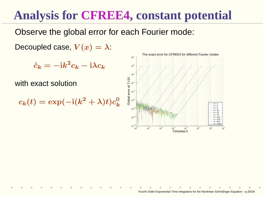
Analysis for CFREE4, constant potentialObserve the global error for each Fourier mode:
Decoupled case, V (x) = λ:
ck = −ik2ck − iλck
with exact solution
ck(t) = exp(−i(k2 + λ)t)c0k
10−6
10−5
10−4
10−3
10−2
10−1
100
101
10−14
10−12
10−10
10−8
10−6
10−4
10−2
100
102
The exact error for CFREE4 for different Fourier modes
Timestep h G
loba
l err
or a
t T=
10
k = 1k = 2k = 4k = 10k = 21k = 47k = 101k = 219k = 474k = 1023
Fourth Order Exponential Time Integrators for the Nonlinear Schrödinger Equation – p.20/24
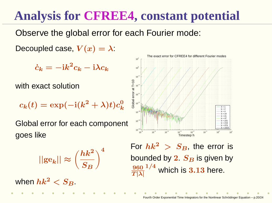
Analysis for CFREE4, constant potentialObserve the global error for each Fourier mode:
Decoupled case, V (x) = λ:
ck = −ik2ck − iλck
with exact solution
ck(t) = exp(−i(k2 + λ)t)c0k
Global error for each component
goes like
||gek|| ≈
(
hk2
SB
)4
when hk2 < SB.
10−6
10−5
10−4
10−3
10−2
10−1
100
101
10−14
10−12
10−10
10−8
10−6
10−4
10−2
100
102
The exact error for CFREE4 for different Fourier modes
Timestep h G
loba
l err
or a
t T=
10
k = 1k = 2k = 4k = 10k = 21k = 47k = 101k = 219k = 474k = 1023
For hk2 > SB, the error is
bounded by 2. SB is given by960T |λ|
1/4which is 3.13 here.
Fourth Order Exponential Time Integrators for the Nonlinear Schrödinger Equation – p.20/24
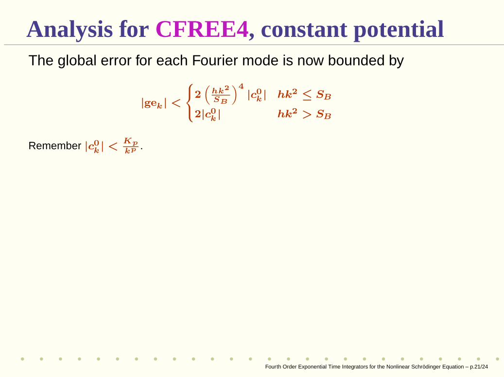
Analysis for CFREE4, constant potentialThe global error for each Fourier mode is now bounded by
|gek| <
8
<
:
2“
hk2
SB
”4|c0
k| hk2 ≤ SB
2|c0k| hk2 > SB
Remember |c0k| <
Kp
kp .
Compute
1
4||gek||22 =
1
4
NF /2−1X
k=−NF /2
|gek|2
≤X
|k|≤√
Sb/h
„
hk2
SB
«8
|c0k|2 +
X
|k|>√
SB/h
|c0k|2
≤ K2p
„
h
Sb
«8X
|k|≤√
SB/h
k16−2p + K2p
X
|k|>√
SB/h
k−2p
Using the Euler–MacLaurin with remainder term to find bounds for the sums, weeventually find forp ≤ 8
||ge||2 ≤ K
„
h
SB
«
2p−1
4
Fourth Order Exponential Time Integrators for the Nonlinear Schrödinger Equation – p.21/24
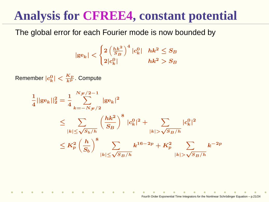
Analysis for CFREE4, constant potentialThe global error for each Fourier mode is now bounded by
|gek| <
8
<
:
2“
hk2
SB
”4|c0
k| hk2 ≤ SB
2|c0k| hk2 > SB
Remember |c0k| <
Kp
kp . Compute
1
4||gek||22 =
1
4
NF /2−1X
k=−NF /2
|gek|2
≤X
|k|≤√
Sb/h
„
hk2
SB
«8
|c0k|2 +
X
|k|>√
SB/h
|c0k|2
≤ K2p
„
h
Sb
«8X
|k|≤√
SB/h
k16−2p + K2p
X
|k|>√
SB/h
k−2p
Using the Euler–MacLaurin with remainder term to find bounds for the sums, weeventually find forp ≤ 8
||ge||2 ≤ K
„
h
SB
«
2p−1
4
Fourth Order Exponential Time Integrators for the Nonlinear Schrödinger Equation – p.21/24
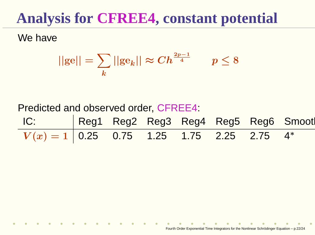
Analysis for CFREE4, constant potentialWe have
||ge|| =∑
k
||gek|| ≈ Ch2p−1
4 p ≤ 8
Predicted and observed order, CFREE4:IC: Reg1 Reg2 Reg3 Reg4 Reg5 Reg6 SmoothV (x) = 1 0.25 0.75 1.25 1.75 2.25 2.75 4∗
Fourth Order Exponential Time Integrators for the Nonlinear Schrödinger Equation – p.22/24
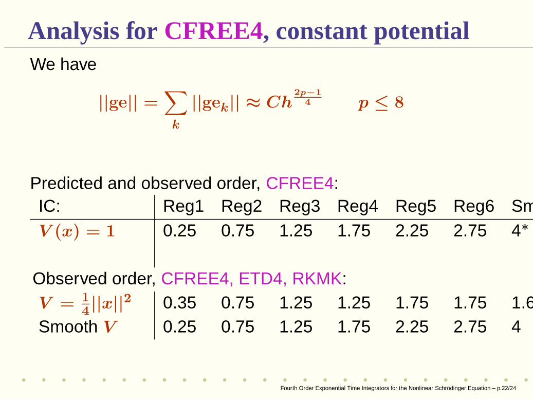
Analysis for CFREE4, constant potentialWe have
||ge|| =∑
k
||gek|| ≈ Ch2p−1
4 p ≤ 8
Predicted and observed order, CFREE4:IC: Reg1 Reg2 Reg3 Reg4 Reg5 Reg6 SmoothV (x) = 1 0.25 0.75 1.25 1.75 2.25 2.75 4∗
Observed order, CFREE4, ETD4, RKMK:V = 1
4||x||2 0.35 0.75 1.25 1.25 1.75 1.75 1.65
Smooth V 0.25 0.75 1.25 1.75 2.25 2.75 4
Fourth Order Exponential Time Integrators for the Nonlinear Schrödinger Equation – p.22/24
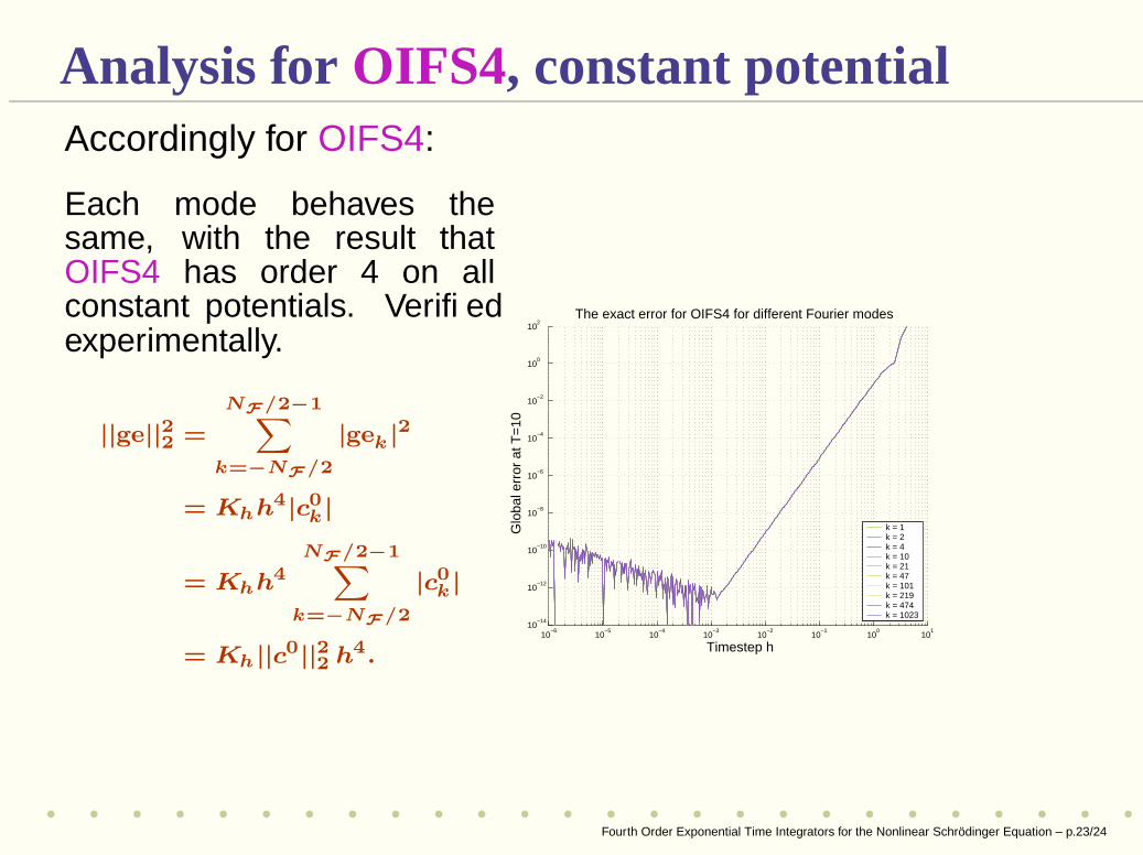
Analysis for OIFS4, constant potentialAccordingly for OIFS4:
Each mode behaves thesame, with the result thatOIFS4 has order 4 on allconstant potentials. Verifiedexperimentally.
||ge||22 =
NF /2−1X
k=−NF /2
|gek|2
= Khh4|c0k|
= Khh4NF /2−1
X
k=−NF /2
|c0k|
= Kh||c0||22 h4.10
−610
−510
−410
−310
−210
−110
010
110
−14
10−12
10−10
10−8
10−6
10−4
10−2
100
102
The exact error for OIFS4 for different Fourier modes
Timestep h
Glo
bal e
rror
at T
=10
k = 1k = 2k = 4k = 10k = 21k = 47k = 101k = 219k = 474k = 1023
Fourth Order Exponential Time Integrators for the Nonlinear Schrödinger Equation – p.23/24
The endReferences
• See Borko & Will’s slides for a reference list..
Conclusions (or an attempt thereat)
• OIFS seems best for our Schrödinger application
Fourth Order Exponential Time Integrators for the Nonlinear Schrödinger Equation – p.24/24
The endReferences
• See Borko & Will’s slides for a reference list..
Conclusions (or an attempt thereat)
• OIFS seems best for our Schrödinger application
Fourth Order Exponential Time Integrators for the Nonlinear Schrödinger Equation – p.24/24

![3. Regression & Exponential Smoothinghpeng/Math4826/Chapter3.pdf · Discounted least squares/general exponential smoothing Xn t=1 w t[z t −f(t,β)]2 • Ordinary least squares:](https://static.fdocument.org/doc/165x107/5e941659aee0e31ade1be164/3-regression-exponential-hpengmath4826chapter3pdf-discounted-least-squaresgeneral.jpg)