Fourier transformFourier transform

{ }{ }1

( , ) ( , )exp 2 ( )

( , )

x y x y x y

x y

f x y g f f j xf yf df df

g f f

π+∞−∞

−

= +∫ ∫

= F

{ }{ }

( , ) ( , )exp 2 ( )

( , )x y x yg f f f x y j f x f y dxdy

f x y

π+∞−∞= − +

=

∫ ∫F

( , ) ( , )

( , ) ( , )

FT IFT

x y

x y

f x y g f f

f x y g f f

⇒

⇐

Introduction to Fourier Optics, J. GoodmanFundamentals of Photonics, B. Saleh &M. Teich

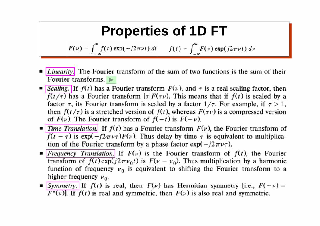
Properties of 1D FTProperties of 1D FT

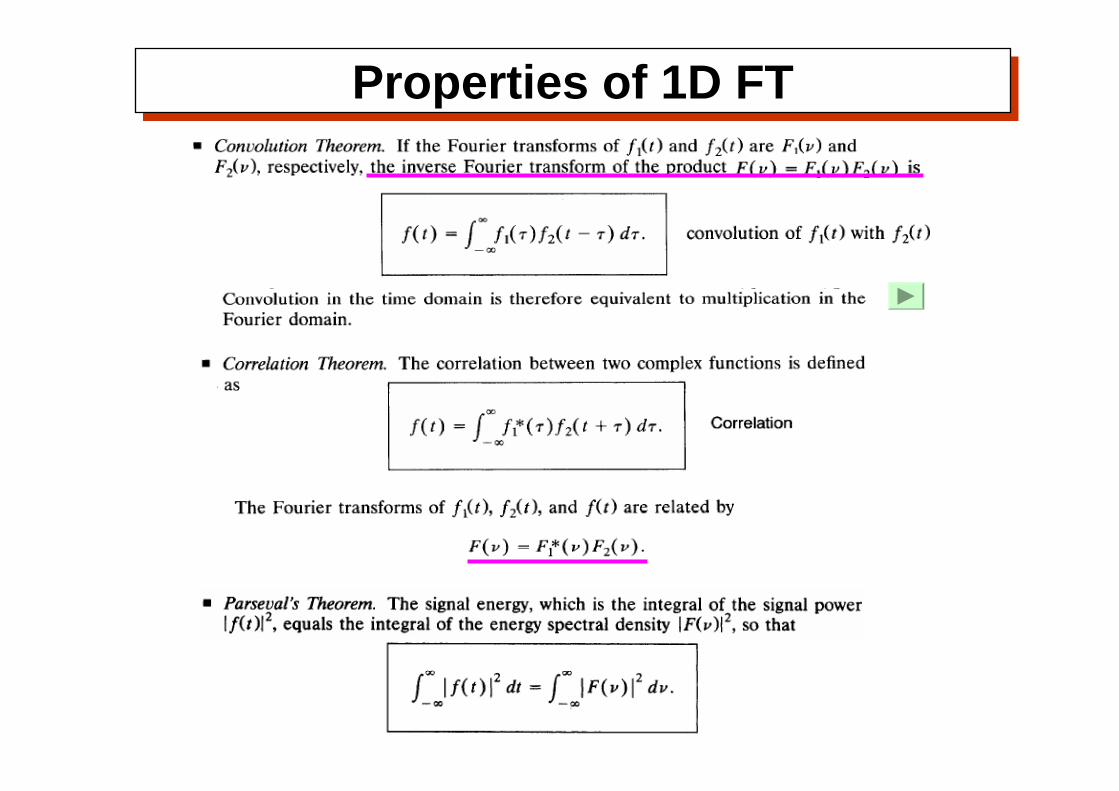
Properties of 1D FTProperties of 1D FT

Some frequently used functionsSome frequently used functions

Some frequently used functionsSome frequently used functions

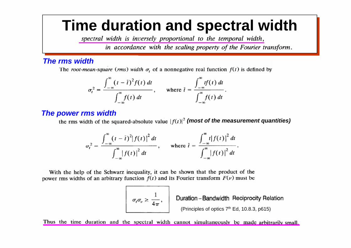
Time duration and spectral widthTime duration and spectral width

The power rms width(most of the measurement quantities)

The rms width

(Principles of optics 7th Ed, 10.8.3, p615)

Time duration and spectral widthTime duration and spectral width

Widths at 1/e, 3-dB, half-maximum Widths at 1/e, 3-dB, half-maximum

1

f(t)

t

= 2τ.

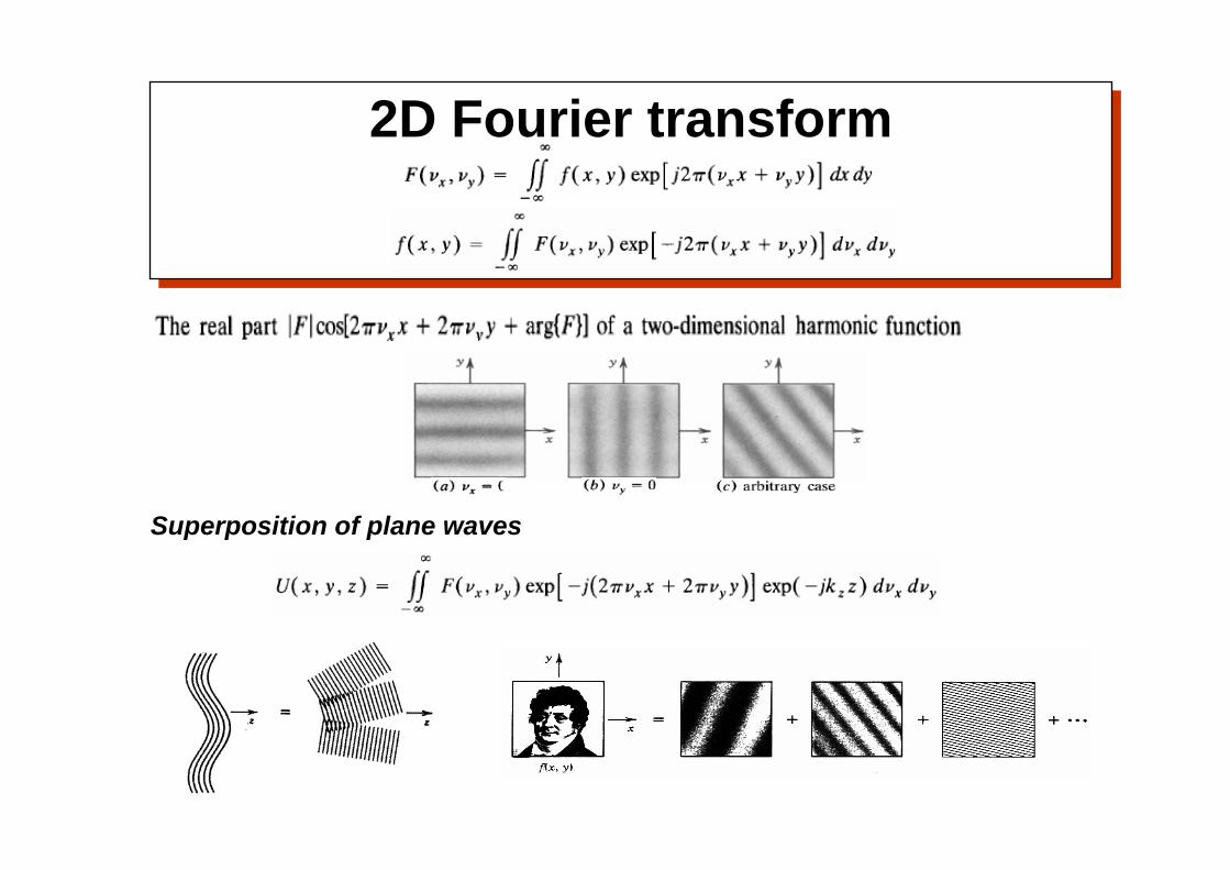
2D Fourier transform2D Fourier transform

Superposition of plane waves

Remind ! Spatial frequency and propagation angleRemind ! Spatial frequency and propagation angle

z

directional cosine : xα λν=

1

xνΛ =

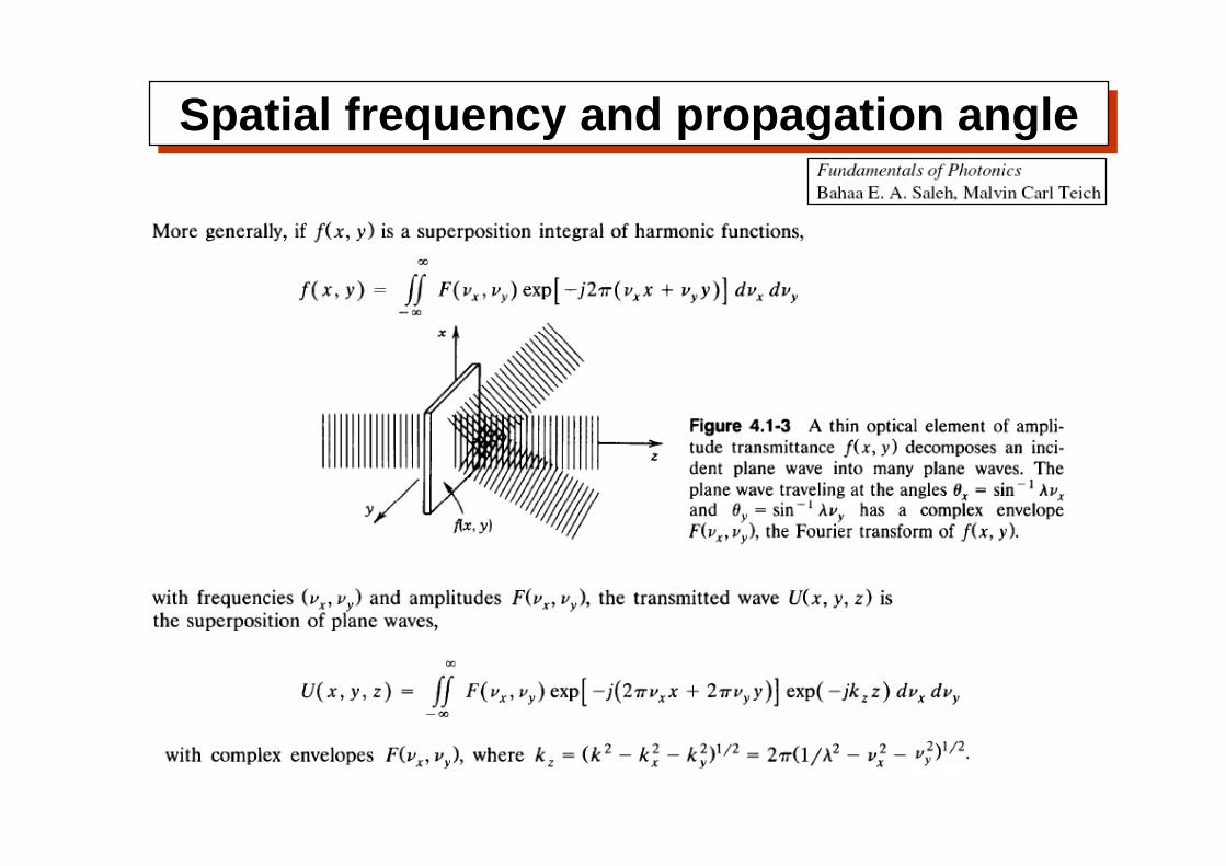
Spatial frequency and propagation angleSpatial frequency and propagation angle

Fourier and Inverse Fourier Transform

α

βα β

( , )x yf f

Properties of 2D FTProperties of 2D FT

Properties of 2D FTProperties of 2D FT

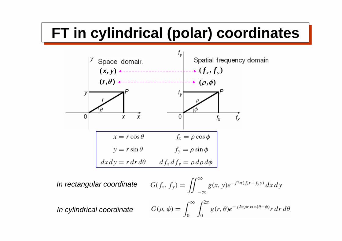
FT in cylindrical (polar) coordinatesFT in cylindrical (polar) coordinates

In rectangular coordinate

In cylindrical coordinate

( , )( , )x yr θ

( , )

( , )x yf f

ρ φ

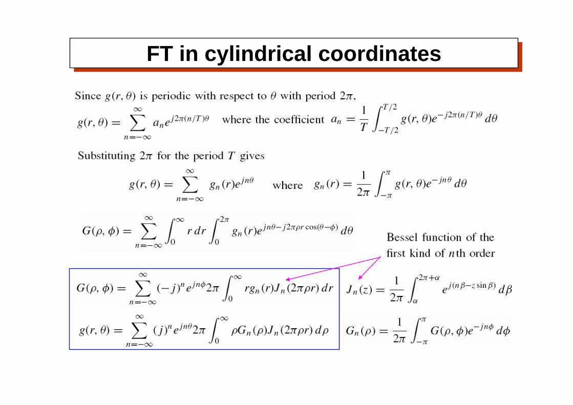
FT in cylindrical coordinatesFT in cylindrical coordinates

FT in cylindrical coordinatesFT in cylindrical coordinates

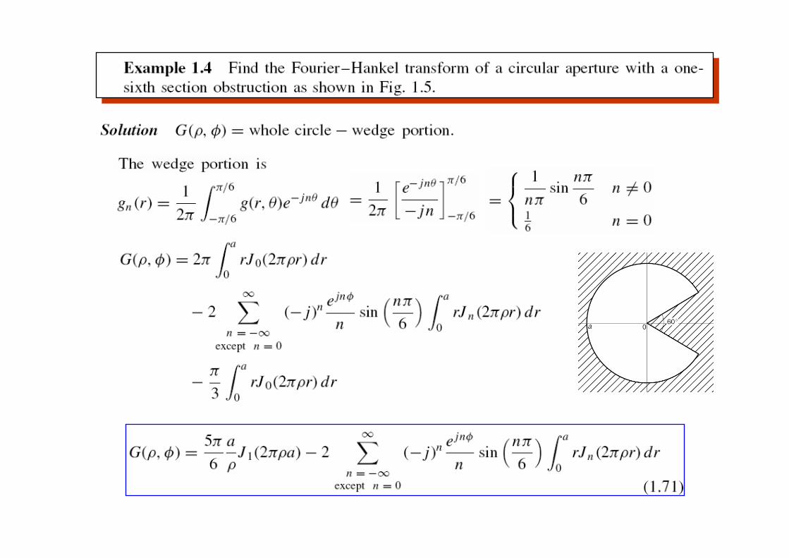
(Ex) Circular aperture : for the special case when

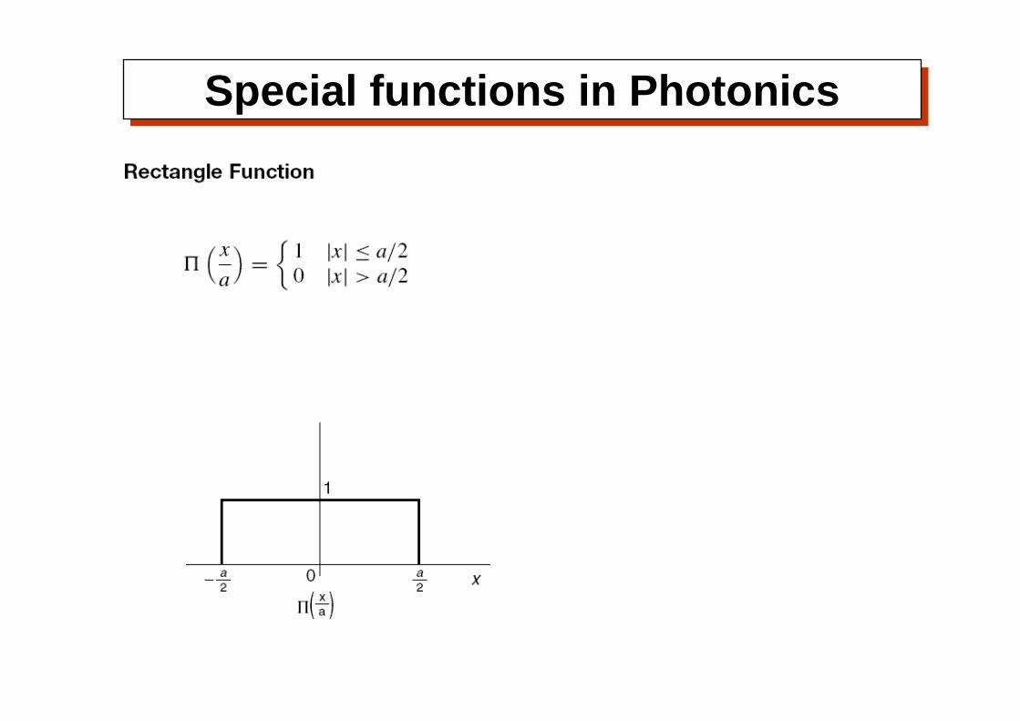
Special functions in PhotonicsSpecial functions in Photonics

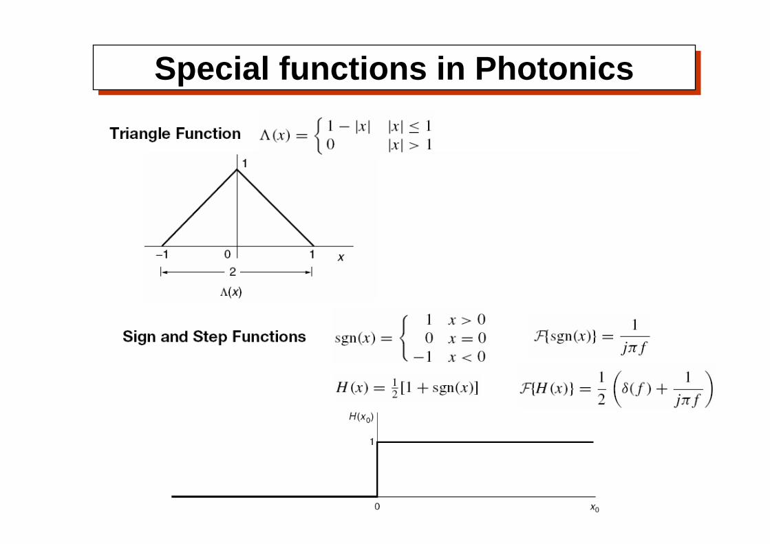
Special functions in PhotonicsSpecial functions in Photonics

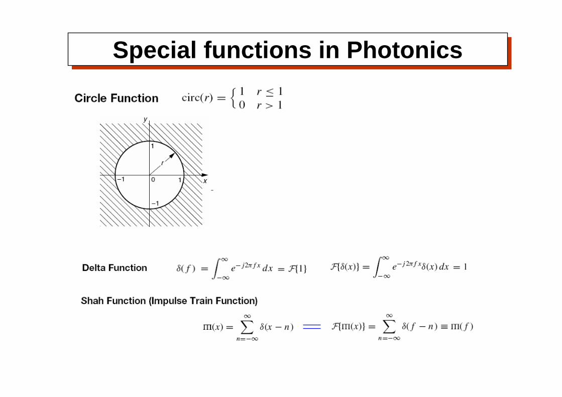
Special functions in PhotonicsSpecial functions in Photonics

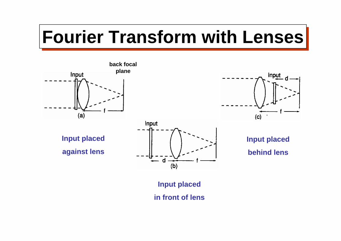
Input placed

against lens

Input placed

in front of lens

Input placed

behind lens

back focal plane

Fourier Transform with LensesFourier Transform with Lenses

R1>0 (concave)R2<0 (convex)

( ) ( ) ( )[ ]yxkyxknyx ,,, 0 Δ−Δ+Δ=φ

( ) [ ] ( ) ( )[ ]yxnjkjkyxtl ,1expexp, 0 Δ−Δ=

( ) ( ) ( )yxUyxtyxU lll ,,,' =

( )⎥⎥⎦

⎤

⎢⎢⎣

⎡ +−−+

⎥⎥⎦

⎤

⎢⎢⎣

⎡ +−−−Δ=Δ 2

2

22

221

22

10 1111,R

yxRR

yxRyx

A thin lens as a phase transformationA thin lens as a phase transformation

( )' ,lU x y( ),lU x y

Intro. to Fourier Optics, Chapter 5, Goodman.

The Paraxial Approximation

( ) [ ] ( ) ⎥⎦

⎤⎢⎣

⎡⎟⎟⎠

⎞⎜⎜⎝

⎛−

+−−Δ=

21

22

011

21expexp,

RRyxnjkjknyxtl

( ) ⎟⎟⎠

⎞⎜⎜⎝

⎛−−≡

21

1111RR

nf

concave:0<fconvex:0>f

( ) ( )⎥⎦

⎤⎢⎣

⎡+−= 22

2exp, yx

fkjyxtl

Phase representation of a thin lens (paraxial approximation)

focal length

Types of Lensesconvex:0>f

concave:0<f

( ) ( )⎥⎦

⎤⎢⎣

⎡+−= 22

2exp, yx

fkjyxtl

Collimating property of a convex lensCollimating property of a convex lens

Fig. 1.21, Iizuka

zi

Plane wave!

How can a convex lens perform the FTHow can a convex lens perform the FT

fo fo

Fourier transforming property of a convex lensFourier transforming property of a convex lensThe input placed directly against the lens

Pupil function ; ( ) 1 in side the lens aperture,

0 otherw iseP x y

⎧= ⎨⎩

( ) ( ) ( ) ( )' 2 2, , , exp2l lkU x y U x y P x y j x yf

⎡ ⎤= − +⎢ ⎥

⎣ ⎦

( )( )

( ) ( ) ( )2 2

' 2 2

exp2 2, , exp exp

2f l

kj uf kU u U x y j x y j xu y dxdyj f f f

υπυ υ

λ λ

∞

−∞

⎡ ⎤+⎢ ⎥ ⎡ ⎤ ⎡ ⎤⎣ ⎦= + − +⎢ ⎥ ⎢ ⎥

⎣ ⎦ ⎣ ⎦∫ ∫

( )( )

( ) ( ) ( )2 2exp

2 2, , , expf l

kj uf

U u U x y P x y j xu y dxdyj f f

υπυ υ

λ λ

∞

−∞

⎡ ⎤+⎢ ⎥ ⎡ ⎤⎣ ⎦= − +⎢ ⎥

⎣ ⎦∫ ∫

Quadratic phase factor

From the Fresnel diffraction formula ( z = f ):

Fourier transform

Fourier transforming property of a convex lensFourier transforming property of a convex lensThe input placed in front of the lens

( )( )

( ) ( )2 2exp 1

2 2, , expf l

k dA j uf f

U u U x y j xu y dxdyj f f

υπυ υ

λ λ

∞

−∞

⎡ ⎤⎛ ⎞− +⎢ ⎥⎜ ⎟ ⎡ ⎤⎝ ⎠⎣ ⎦= − +⎢ ⎥

⎣ ⎦∫ ∫

If d = f

( ) ( ) ( )2, , expf lAU u U x y j xu y dxdy

j f fπυ υ

λ λ

∞

−∞

⎡ ⎤= − +⎢ ⎥

⎣ ⎦∫ ∫

Exact Fourier transform !

( )( )

df

dj

udkjA

uU f λ

υυ

⎥⎦⎤

⎢⎣⎡ +

=

22

2exp

, ( ) ( ) ηξυηξλπηξηξ ddud

jdf

dfPtA ⎥⎦

⎤⎢⎣⎡ +−⎟

⎠⎞

⎜⎝⎛× ∫ ∫

∞

∞−

2exp,,

Fourier transforming property of a convex lensFourier transforming property of a convex lensThe input placed behind the lens

Scaleable Fourier transform !

By decreasing d, the scale of the transform is made smaller.

( ) ( ) ( )ηξηξηξηξ , 2

exp,, 220 Atd

kjdf

dfP

dAfU

⎭⎬⎫

⎩⎨⎧

⎥⎦⎤

⎢⎣⎡ +−⎟

⎠⎞

⎜⎝⎛=

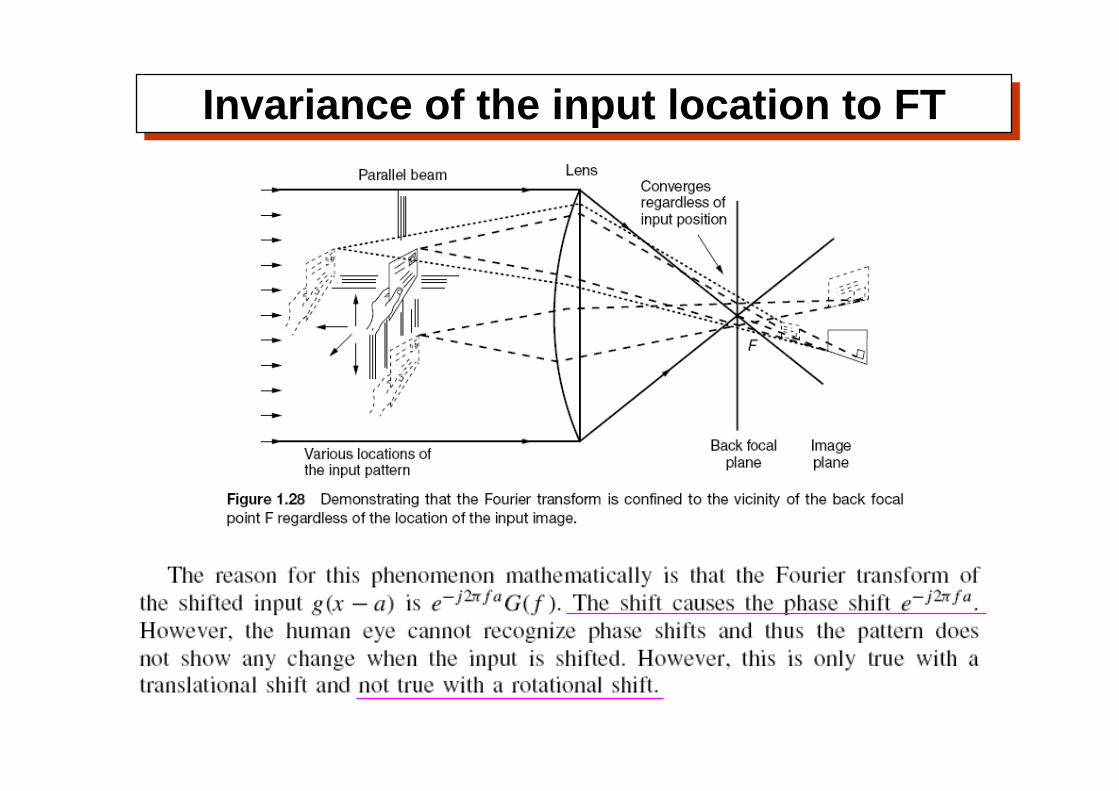
Invariance of the input location to FTInvariance of the input location to FT

Imaging property of a convex lensImaging property of a convex lens

magnification

From an input point S to the output point P ;

Fig. 1.22, Iizuka

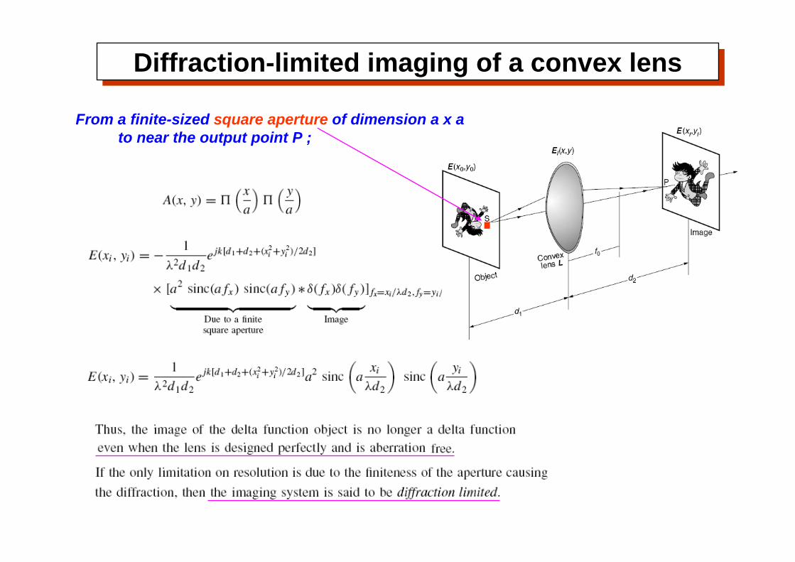
Diffraction-limited imaging of a convex lensDiffraction-limited imaging of a convex lens

From a finite-sized square aperture of dimension a x a to near the output point P ;

Appendix : Linear systemsAppendix : Linear systems

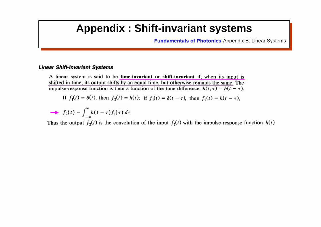
Appendix : Shift-invariant systemsAppendix : Shift-invariant systems

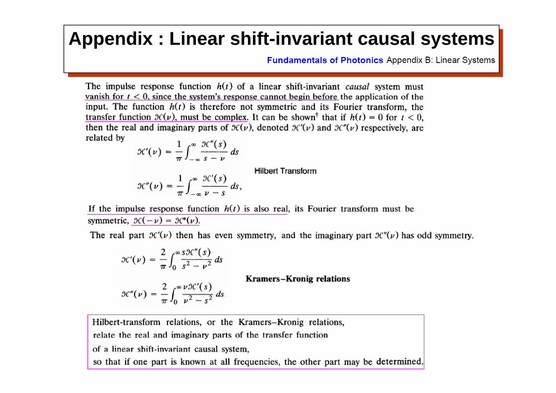
Appendix : Linear shift-invariant causal systemsAppendix : Linear shift-invariant causal systems

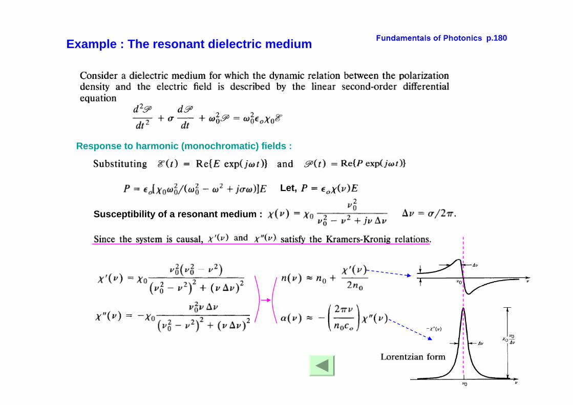
p.180Example : The resonant dielectric medium

Susceptibility of a resonant medium :

Let,

Response to harmonic (monochromatic) fields :

Appendix : Transfer functionAppendix : Transfer function