FORMULATION AND ANALYSIS OF ALTERNATING EVOLUTION (AE) SCHEMES

FORMULATION AND ANALYSIS OF ALTERNATING EVOLUTION (AE)

SCHEMES FOR HYPERBOLIC CONSERVATION LAWS

HASEENA AHMED AND HAILIANG LIU

Abstract. The alternating evolution (AE) system of Liu [22]

∂tu + ∂xf(v) =1

ǫ(v − u), ∂tv + ∂xf(u) =

1

ǫ(u − v),

is an accurate approximation to systems of hyperbolic conservation laws

∂tφ + ∂xf(φ) = 0, φ(x, 0) = φ0(x).

In particular, when two components take the same initial value as φ0, the exact solution of conser-vation laws is precisely captured by the approximate system.

In this paper we develop a class of local Alternating Evolution (AE) schemes, where we takeadvantage of high accuracy of the AE approximation. Our approach is based on a sliding averageof the AE system over an interval of [x − ∆x, x + ∆x]. The numerical scheme is then constructedby sampling the averaged system over alternating grids. Higher order accuracy is achieved by acombination of high-order polynomial reconstruction from the obtained averages and a stable Runge-Kutta discretization in time. Local AE schemes are made possible by letting the scale parameterǫ reflect the local distribution of nonlinear waves. The AE schemes have the advantage of easierformulation and implementation, and efficient computation of the solution. For the first and secondorder local AE schemes applied to scalar laws, we prove the numerical stability in the sense ofsatisfying the maximum principle and total variation diminishing (TVD) property. Numerical testsfor both scalar conservation laws and compressible Euler equations are presented to demonstrate thehigh order accuracy and capacity of these AE schemes.

Contents

1. Introduction 12. Scheme formulation 32.1. Global AE schemes 32.2. Local AE schemes 53. Stability analysis 83.1. Stability of first order AE schemes 83.2. Stability of second order AE schemes 104. Numerical tests 134.1. Scalar conservation laws 134.2. Euler equations of gas dynamics 175. Concluding remarks 20Acknowledgments 20References 31

Date: version December 18, 2007.1991 Mathematics Subject Classification. 35L65, 65M06.Key words and phrases. Conservation laws, Alternating evolution schemes, Shock capturing methods, TVD stability.

1

2 HASEENA AHMED AND HAILIANG LIU

1. Introduction

A multi-D hyperbolic conservation law (CL) has the form:

(1.1) φt + ∇x · f(φ) = 0, x ∈ Rd, t > 0,

where φ ∈ Rm denotes a vector of conserved quantities, and f : R

m → Rd is a nonlinear convection

flux. The compressible Euler equation in gas dynamics is a canonical example. These equationsare of great practical importance since they model a variety of physical phenomena that appear influid mechanics, astrophysics, groundwater flow, traffic flow, semiconductor device simulation, andmagneto-hydrodynamics, among many others.

The need for devising accurate and efficient numerical methods for nonlinear hyperbolic conserva-tion laws and related models has prompted and sustained the abundant research in this area, see, forexample, [19, 31, 3]. The notorious difficulty encountered for the satisfactory approximation of theexact solutions of these systems lies in the presence of discontinuities in the solution. A well knownrecipe to achieve both high-order accuracy and convergence to the entropy solution is the so calledhigh-resolution schemes. The success has been due to two factors: the local enforcement of nonlinearconservation laws and the non-oscillatory piecewise polynomial reconstruction from evolved localmoments (cell averages).

In this work we present new alternating evolution (AE) schemes to (1.1), together with stabilityanalysis and performance test through numerical experiments. These schemes can be viewed asmodifications of the global AE scheme proposed in [22]. In the formulation of these schemes weborrow techniques of both the local enforcement and the high-order polynomial reconstruction fromthe literature, but apply them to a novel approximation system, which in one-dimensional case reads

ut + ∇x · f(v) =1

ǫ(v − u),(1.2)

vt + ∇x · f(u) =1

ǫ(u − v).(1.3)

Here ǫ > 0 is a scale parameter of user’s choice. One distinguished feature of this approximate systemis its extremely high accuracy; for scalar conservation laws it is proven that this system capturesthe exact entropy solution for nonlinear conservation laws provided both components take the sameinitial data as the one given for the conservation law, i.e., if initially u(x, 0) = v(x, 0) = φ0(x), then

u(x, t) = v(x, t) = φ(x, t), ∀ (x, t) ∈ Rd × R

+.

The convergence results for the solution of the approximate system to the entropy solution of theconservation law can be found in detail in [22]. On the other hand if the system is rewritten as

u + ǫut = v − ǫ∇x · f(v), v + ǫvt = u − ǫ∇x · f(u),

one can see for ǫ = O(∆t) the system is able to transfer spatial changes of one component intotemporal changes of another component. The communication between two components is thusrealized by the choice of parameter ǫ. This was illustrated in [22] for linear scalar conservation lawswith constant speed a

(1.4) φt + aφx = 0, φ(x, 0) = φ0(x), x ∈ R1, t > 0

having an explicit solution φ(x, t) = φ0(x − at). The AE approximation system has the followingexact solution

u(x, t) =1

2u0(x − at)(1 + e−4t/ǫ) +

1

2v0(x − at)(1 − e−4t/ǫ),

v(x, t) =1

2u0(x − at)(1 − e−4t/ǫ) +

1

2v0(x − at)(1 + e−4t/ǫ).

From this we see that u−v converges exponentially to zero as ǫ becomes small even when u0−v0 6= 0.

AE SCHEMES FOR HYPERBOLIC CONSERVATION LAWS 3

The numerical schemes, presented in [22] and this work, take advantage of these remarkablefeatures of the AE system. There are three steps involved in the discretization procedure: (i) theapproximate system is locally enforced by taking the spatial averaging over [x−∆x, x+∆x]; (ii) theaveraged system is then sampled over alternating grids for its two components; (iii) the piecewisepolynomial reconstruction from averages of two components is carried out, respectively, followed bythe Runge-Kutta method for time discretization of the resulting semi-discrete system. Extension ofthis procedure to multi-dimensional problems is straightforward. The scheme obtained in this manneris thus called the alternating evolution (AE) scheme. Another attractive feature of the AE schemeis the amount of leverage in the choice of ǫ. Indeed different choices of the scale parameter in such aprocedure yield a class of AE schemes. In addition, the method is not restricted to only conservationlaws. An extension of the numerical approach to Hamilton Jacobi equations is in progress.

To put our study in the proper perspective we recall a few of the references from the considerableamount of literature available on numerical methods for hyperbolic conservation laws. The finitedifference/volume solution techniques for nonlinear conservation laws fall under two main categoriesaccording to their way of sampling [27]: upwind and central schemes. The forerunners for these twolarge classes of high resolution schemes for nonlinear conservation laws are the first-order Godunov[7] and Lax-Friedrichs (LxF) schemes [6, 18], respectively.

In [7] Godunov proposed to evolve a piecewise cell average representation of the solution andevaluate the fluxes at cell interfaces. Godunov type upwind schemes are then obtained by using anexact or approximate Riemann solver to distribute the non-linear waves between two neighboringcomputational cells. Various higher-order extensions of the Godunov scheme have been rapidlydeveloped since 1970’s, employing higher-order reconstruction of piece-wise polynomials from thecell averages, including MUSCL, TVD, PPM, ENO and WENO schemes [32, 33, 8, 4, 9, 29, 30, 23].

In contrast, Godunov type central schemes are more diffusive, yet easy to formulate and implementsince no Riemann solvers are required. In the one-dimensional case, examples of such schemes forconservation laws are the second-order Nessyahu-Tadmor scheme [27] and the higher-order schemesin [24, 2, 20]. Second-order multi-D central schemes were introduced in [11], and their higher-orderextensions were developed in [16], among others.

The two categories of schemes are somehow interlaced during their independent developments;the upwind scheme becomes Riemann solver-free when a local numerical flux is used to replace theexact Riemann solver, see Shu and Osher [29, 30], and the central scheme becomes less diffusivewhen variable control volumes are used in deriving the scheme, see Kurganov and Tadmor [17]. Theupwind feature can be further enforced [10, 15].

We note that an alternative technique to control the numerical dissipation in central schemes wasrecently developed by Liu [25]. In his procedure, a convex combination of central schemes involvingtwo overlapping cell averages is utilized.

The scheme that we design here is different in that it is based on discretization of the AE ap-proximation [22], which has no method error for well-prepared initial data. Two representations ofthe solution are evolved on alternating grids. The solution of the AE approximation is as regularas the entropy solution, no additional stability condition needs to be imposed to drive approximatestates to the entropy solution of conservation laws. In this aspect the AE approximation systemalso distinguishes itself from other existing approximations to nonlinear conservation laws, such asthe viscous approximation [14], the kinetic approximation [28, 21], and the relaxation approximation[12, 13, 26].

Finally we mention that the ideas of numerical fluxes coined in the development of high resolutionschemes when incorporated into a finite element space discretization by discontinuous approximationshave resulted in a rapid development of compact high resolution schemes in recent years, see, forexample, the RKDG methods by Cockburn and Shu [3], and the spectral volume methods by Wang[34].


We now conclude this section by outlining the rest of the paper. In section 2 we give the first andsecond order formulation of the numerical method for both the global and local schemes. Under someCFL type conditions, both the TVD property and the maximum principle are proved in section 3 forfirst and second order local AE schemes, respectively. Numerical tests for both scalar conservationlaws and compressible Euler equations for 1st, 2nd and 3rd order schemes are presented in section4. Our numerical results show that the AE schemes can capture shock waves as well as other highresolution schemes.

2. Scheme formulation

The detailed formulation and stability analysis of the first and second order global AE scheme isgiven in [22]. We present the idea here again.

2.1. Global AE schemes. Let u(x, t) denote the sliding average of u(·, t) over interval Ix = {ξ| x−∆x ≤ ξ ≤ x + ∆x}:

u(x, t) =1

2∆x

∫ x+∆x

x−∆xu(ξ, t)dξ.

Integration of the 1-D AE system (1.2)-(1.3) over Ix gives

d

dtu(x, t) = −

u(x, t)

ǫ+

1

ǫL[v](x, t),(2.1)

d

dtv(x, t) = −

v(x, t)

ǫ+

1

ǫL[u](x, t),(2.2)

where x serves as a moving parameter and

(2.3) L[Φ](x, t) = Φ(x, t) −ǫ

2∆x(f(Φ(x + ∆x, t)) − f(Φ(x − ∆x, t))) .

The numerical scheme is constructed by sampling both formulations (2.1) and (2.2) over alternatinggrids for u and v, respectively, with proper approximation of L[Φ] defined in (2.3). For example, ifwe sample (2.1) at x2j and (2.2) at x2j+1, respectively, then we have

d

dtu2j(t) =

1

ǫ[−u2j(t) + L2j [v](t)],(2.4)

d

dtv2j+1(t) =

1

ǫ[−v2j+1(t) + L2j+1[u](t)].(2.5)

Here we define Lk[Φ](t) := L[Φ](xk, t). In general, the total numerical solution at time tn = n∆t canbe written as

(2.6) Φnk =

{

unk k = 2j,

vnk k = 2j + 1.

The high accuracy of the scheme is realized via two steps: high-order spatial reconstruction fromaverages Φj and evaluation of L[Φ](t) accordingly; higher-order temporal approximation of the aboveODE system (2.4)-(2.5), such as the Runge-Kutta method.

The piecewise polynomial reconstruction needs to be conservative,

(2.7) Φnk =

1

2∆x

∫

Ik

p[Φn](x) dx,

and should be accurate of desired order, and non-oscillatory. Second order schemes require a piecewiselinear reconstruction. Third order schemes employ a piecewise quadratic approximation. With sucha reconstructed p[Φn], we proceed to evaluate L[Φn] as follows. At any even node k = 2j, usingpiecewise polynomial p[vn] constructed over [x2j , x2j+2] we obtain

(2.8) L2j [vn] =

1

2∆x

∫

I2j

p[vn](x) dx −ǫ

2∆x[f(p[vn]2j+1) − f(p[vn]2j−1)] .


At any odd node k = 2j + 1, using piecewise polynomial p[un] constructed over [x2j−1, x2j+1] weobtain

(2.9) L2j+1[un] =

1

2∆x

∫

I2j+1

p[un](x) dx −ǫ

2∆x[f(p[un]2j+2) − f(p[un]2j)] .

These procedures together with the Runge-Kutta time discretization of the system (2.4)-(2.5) enableus to design a new class of high-resolution schemes for hyperbolic conservation laws, called AEschemes.

2.1.1. First order global AE scheme. In this section, we present the formulation of the first orderglobal AE scheme. If the reconstructed polynomial is piecewise constant, then

1

2∆x

∫

I2j

p[vn](x) dx =vn2j+1 + vn

2j−1

2, and

1

2∆x

∫

I2j+1

p[un](x) dx =un

2j+2 + un2j

2.

The first order scheme then has the form

un+12j = (1 − κ)un

2j + κ

[

vn2j+1 + vn

2j−1

2−

ǫ

2∆x

(

f(vn2j+1) − f(vn

2j−1))

]

,(2.10)

vn+12j+1 = (1 − κ)vn

2j+1 + κ

[

un2j+2 + un

2j

2−

ǫ

2∆x

(

f(un2j+2) − f(un

2j))

]

,(2.11)

where κ = ∆tǫ . The first order scheme is numerically stable if

ǫ

∆xmax |f ′| ≤ 1, the proof of which

can be found in [22]. This scheme when ǫ = ∆t becomes the celebrated Lax Friedrich (LxF) scheme.

2.1.2. Second order global AE scheme. We use a linear polynomial reconstruction of the form

(2.12) p[Φn](x) =∑

k

(Φnk + sn

k(x − xk)) χIk

(x),

where χIk

is the characteristic function which takes value on interval Ik. The non-oscillatory propertyrequires that we choose sn

k with certain limiters. In our schemes we use the basic minmod limiter,see, e.g. [24] and hence

(2.13) snk = minmod

{

Φnk+2 − Φn

k

2∆x,Φn

k − Φnk−2

2∆x

}

,

where

(2.14) minmod {a, b} =1

2(sgn(a) + sgn(b))min{|a|, |b|}.

With the above reconstruction, we obtain

1

2∆x

∫

Ik

p[Φn](x) dx =Φn

k+1+ Φn

k−1

2+

∆x

4(sn

k−1 − snk+1),

so that

(2.15) Lk[Φn] :=

[

Φnk+1

+ Φnk−1

2+

∆x

4(sn

k−1 − snk+1) −

ǫ

2∆x

(

f(Φnk+1) − f(Φn

k−1))

]

.


Using second order Runge-Kutta time discretization, we arrive at the following second order AEscheme

u∗2j = (1 − κ)un

2j + κL2j [vn],(2.16)

v∗2j+1 = (1 − κ)vn2j+1 + κL2j+1[u

n],(2.17)

un+12j =

1

2un

2j +1

2

(

(1 − κ)u∗2j + κL2j [v

∗])

,(2.18)

vn+12j+1 =

1

2vn2j+1 +

1

2

(

(1 − κ)v∗2j+1 + κL2j+1[u∗]

)

.(2.19)

0 0.1 0.2 0.3 0.4 0.5 0.6 0.7 0.8 0.9 10

0.2

0.4

0.6

0.8

1

1.2

1.4

1.6

1.8

2

x

Sol

utio

n u

(a) ǫ = 0.1∆x and ∆t = 0.5ǫ.

0 0.1 0.2 0.3 0.4 0.5 0.6 0.7 0.8 0.9 10

0.2

0.4

0.6

0.8

1

1.2

1.4

1.6

1.8

2

x

Sol

utio

n u

(b) ǫ = 0.01∆x and ∆t = 0.5ǫ.

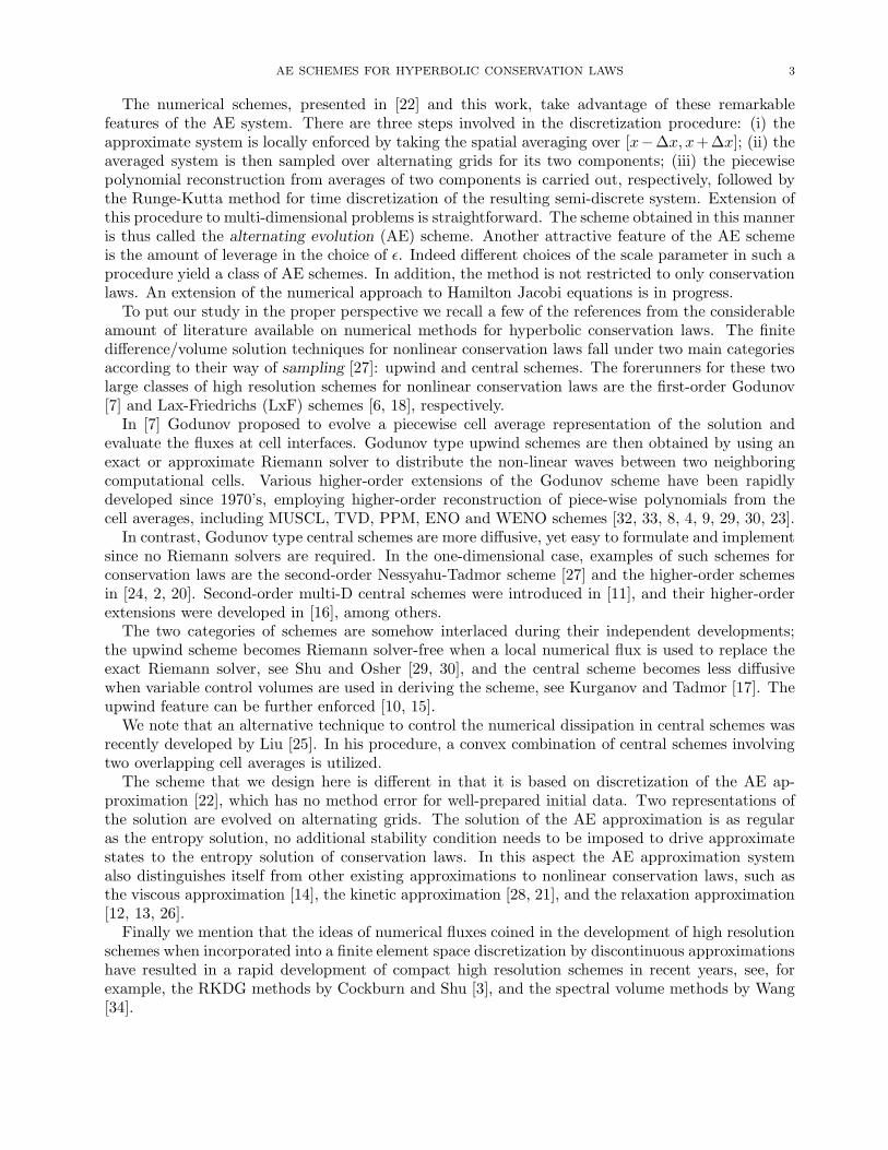
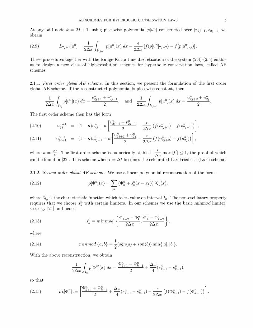
Figure 1: Plot for Burgers’ equation at discontinuity on [0, 2], T = 0.7, N = 200, 2nd order AEscheme to show the effect of change in ǫ.

0 0.1 0.2 0.3 0.4 0.5 0.6 0.7 0.8 0.9 10

0.2

0.4

0.6

0.8

1

1.2

1.4

1.6

1.8

2

x

Sol

utio

n u

(a) ǫ = 0.1∆x and ∆t = 0.5ǫ.

0 0.1 0.2 0.3 0.4 0.5 0.6 0.7 0.8 0.9 10

0.2

0.4

0.6

0.8

1

1.2

1.4

1.6

1.8

2

x

Sol

utio

n u

(b) ǫ = 0.01∆x and ∆t = 0.5ǫ.

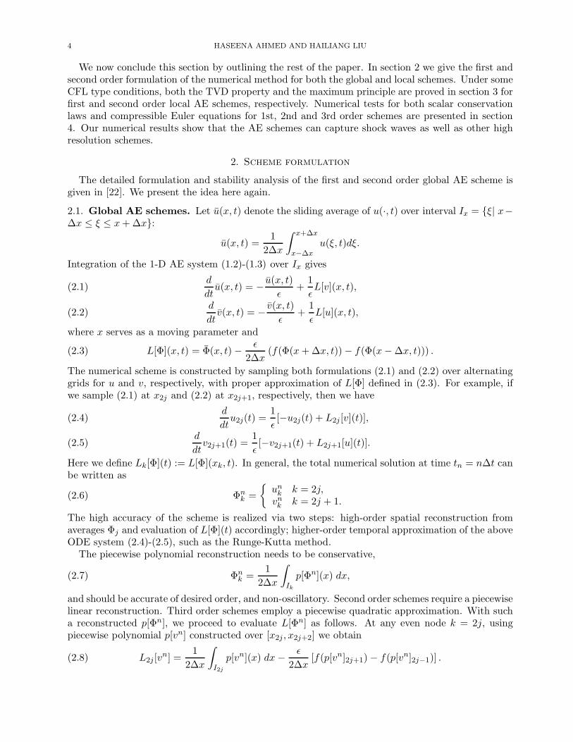
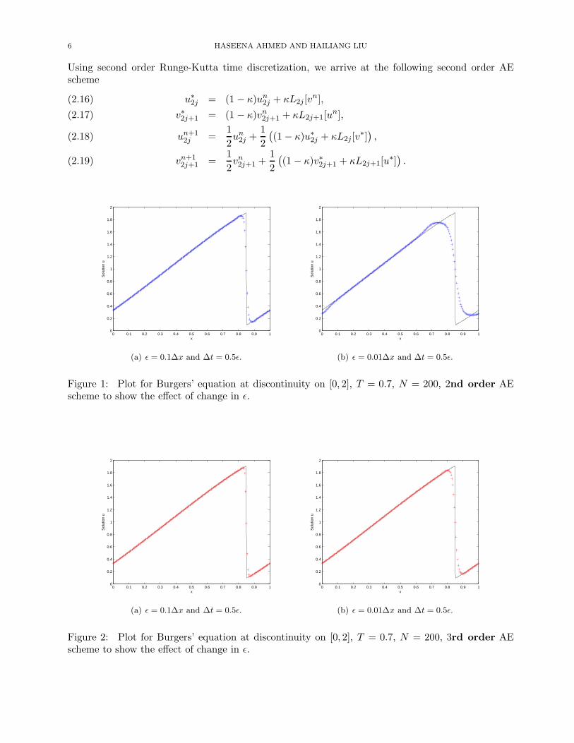
Figure 2: Plot for Burgers’ equation at discontinuity on [0, 2], T = 0.7, N = 200, 3rd order AEscheme to show the effect of change in ǫ.


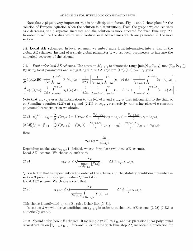
Note that ǫ plays a very important role in the dissipation factor. Fig. 1 and 2 show plots for thesolution of Burgers’ equation when the solution is discontinuous. From the graphs we can see thatas ǫ decreases, the dissipation increases and the solution is more smeared for fixed time step ∆t.In order to reduce the dissipation we introduce local AE schemes which are presented in the nextsection.

2.2. Local AE schemes. In local schemes, we embed more local information into ǫ than in theglobal AE schemes. Instead of a single global parameter ǫ, we use local parameters to increase thenumerical accuracy of the scheme.

2.2.1. First order local AE schemes. Use notation Mk+1/2 to denote the range [min(Φk,Φk+1),max(Φk,Φk+1)].By using local parameters and integrating the 1-D AE system (1.2)-(1.3) over Ix gives

d

dtu(x, t) = −

1

2∆x

∫ x+∆x

x−∆x∂xf(v) dx −

1

2∆x

[

1

ǫx−∆x/2

∫ x

x−∆x(u − v) dx +

1

ǫx+∆x/2

∫ x+∆x

x(u − v) dx

]

,(2.20)

d

dtv(x, t) = −

1

2∆x

∫ x+∆x

x−∆x∂xf(u) dx −

1

2∆x

[

1

ǫx−∆x/2

∫ x

x−∆x(v − u) dx +

1

ǫx+∆x/2

∫ x+∆x

x(v − u) dx

]

.(2.21)

Note that ǫx−∆x/2 uses the information to the left of x and ǫx+∆x/2 uses information to the right ofx. Sampling equation (2.20) at x2j and (2.21) at x2j+1, respectively, and using piecewise constantpolynomial reconstruction we obtain,

un+12j = un

2j −λ

2(f(v2j+1) − f(v2j−1)) −

κ2j−1/2

2(u2j − v2j−1) −

κ2j+1/2

2(u2j − v2j+1),(2.22)

vn+12j+1

= vn2j+1 −

λ

2(f(u2j+2) − f(u2j)) −

κ2j+1/2

2(v2j+1 − u2j) −

κ2j+3/2

2(v2j+1 − u2j+2).(2.23)

Here,

κk+1/2 =∆t

ǫk+1/2

,

Depending on the way ǫk+1/2 is defined, we can formulate two local AE schemes.Local AE1 scheme. We choose ǫk such that

(2.24) ǫk+1/2 ≤ Q∆x

maxs∈Mk+1/2

|f ′(s)|, ∆t ≤ min

kǫk+1/2.

Q is a factor that is dependent on the order of the scheme and the stability conditions presented insection 3 provide the range of values Q can take.Local AE2 scheme. We choose ǫ such that

(2.25) ǫk+1/2 ≤ Q∆x

1

|Mk+1/2|

∫

Mk+1/2

|f ′(s)| ds

, ∆t ≤ mink

ǫk+1/2.

This choice is motivated by the Enguist-Osher flux [5, 31].In section 3 we will derive conditions on ǫk+1/2 in order that the local AE scheme (2.22)-(2.23) is

numerically stable.

2.2.2. Second order local AE schemes. If we sample (2.20) at x2j , and use piecewise linear polynomialreconstruction on [x2j−1, x2j+1], forward Euler in time with time step ∆t, we obtain a prediction for


u as un+∆t2j = u∗

2j which can be given as

u∗2j = un

2j −∆t

2∆x(f(vn

2j+1) − f(vn2j−1))

−∆t

2∆x

1

ǫ2j−1/2

∫ x2j

x2j−1

[

(un2j + sn

2j(x − x2j)) − (vn2j−1 + sn

2j−1(x − x2j−1))]

dx

−∆t

2∆x

1

ǫ2j+1/2

∫ x2j+1

x2j

[

(un2j + sn

2j(x − x2j)) − (vn2j+1 + sn

2j+1(x − x2j+1))]

dx,

= un2j −

∆t

2∆x(f(vn

2j+1) − f(vn2j−1)) −

∆t

2ǫ2j−1/2

(

un2j − vn

2j−1 −∆x

2(sn

2j + sn2j−1)

)

−∆t

2ǫ2j+1/2

(

un2j − vn

2j+1 +∆x

2(sn

2j + sn2j+1)

)

,

= un2j − ∆tL2j[u

n, vn],

where

Lk[u, v] =1

2∆x(f(vk+1) − f(vk−1)) +

1

2ǫk−1/2

(

uk − vk−1 −∆x

2(sk + sk−1)

)

+1

2ǫk+1/2

(

uk − vk+1 +∆x

2(sk + sk+1)

)

.

Similarly we can sample (2.21) at x2j+1 and use piecewise linear polynomial reconstruction to obtain

a prediction for vn+∆t2j+1 = v∗2j+1. Using second order Runge-Kutta time discretization, we arrive at

the second order scheme

u∗2j = un

2j − ∆tL2j [un, vn],(2.26)

v∗2j+1 = vn2j+1 − ∆tL2j+1[v

n, un],(2.27)

un+12j =

1

2un

2j +1

2u∗

2j −∆t

2L2j[u

∗, v∗],(2.28)

vn+12j+1 =

1

2vn2j+1 +

1

2v∗2j+1 −

∆t

2L2j+1[v

∗, u∗].(2.29)

Second order local AE1 and AE2 schemes are designed as in the case of local first order AE schemes.Next we make some remarks regarding the properties of the scheme.

Remark 2.1. Conservative form: The local AE schemes are conservative. i.e., it satisfies,

d

dt(u + v) = 0.

We can check this for the first order scheme by

∑

k even

un+1

k + vn+1

k+1=

∑

k even

{

unk −

∆t

2∆x(f(vk+1) − f(vk−1)) −

κk−1/2

2(uk − vk−1) −

κk+1/2

2(uk − vk+1)

+vnk+1 −

∆t

2∆x(f(uk+2) − f(uk)) −

κk+1/2

2(vk+1 − uk) −

κk+3/2

2(vk+1 − uk+2)

}

=∑

k even

unk + vn

k+1.

Similarly we can show that the conservative property is preserved for higher order schemes we proposein this paper.


Remark 2.2. Numerical viscosity: The local AE2 scheme has the smallest numerical viscosity sinceit uses the average of the local speed over a cell, followed by the local AE1 scheme which uses themaximum of the local speed over a cell, followed by the global AE scheme which takes the maximumof the speed over all cells.

3. Stability analysis

We state the following theorem to show that the first order scheme is stable in the sense ofsatisfying the maximum principle and total variation diminishing property. Let Φ := {un, vn} be acomputed solution. We use the following notations:

|un|∞ = maxk even

|Φnk |, |vn|∞ = max

k odd|Φn

k |, and |Φn|∞ = max{|un|∞, |vn|∞}.

Also, the total variation

(3.1) TV [Φn] =∑

k even

|Φnk+1 − Φn

k | +∑

k even

|Φnk − Φn

k−1|.

3.1. Stability of first order AE schemes.

Theorem 3.1. Let Φ := {un, vn} be computed from the first order global AE scheme (2.10)-(2.11)for scalar hyperbolic conservation laws. If both

(3.2)ǫ

∆xmax |f ′| ≤ 1 and ∆t ≤ ǫ

hold, then

(3.3) |Φn+1|∞ ≤ |Φn|∞, n ∈ N.

Also,

(3.4) TV [Φn+1] ≤ TV [Φn], n ∈ N.

Proof. See Theorem 5.1 in [22].

Theorem 3.2. Let Φ := {un, vn} be computed from the first order local AE scheme (2.22)-(2.23)for scalar hyperbolic conservation laws. If

(a) for local AE1,

(3.5) ǫk+1/2 ≤∆x

maxs∈Mk+1/2

|f ′(s)|, ∆t ≤

1

2min

kǫk+1/2,

(b) or for local AE2,

(3.6) ǫk+1/2 ≤∆x

1

|Mk+1/2|

∫

Mk+1/2

|f ′(s)| ds

, ∆t ≤1

2min

kǫk+1/2

holds, then

(3.7) |Φn+1|∞ ≤ |Φn|∞, n ∈ N.

Moreover, we have

(3.8) TV [Φn+1] ≤ TV [Φn], n ∈ N.


Proof. We can rewrite equation (2.22) with k = 2j as

un+1

k = unk −

λ

2f ′

k+1/2(ξ1)(vnk+1 − un

k) −λ

2f ′

k−1/2(ξ2)(unk − vn

k−1) −κk−1/2

2(un

k − vnk−1)

−κk+1/2

2(un

k − vnk+1),

where λ =∆t

∆x, ξ1 ∈ Mk+1/2 and ξ2 ∈ Mk−1/2 are intermediate values and

(3.9) f ′k+1/2 =

∫ 1

0

f ′(Φk + η(Φnk+1 − Φn

k)) dη.

Re-arranging, we obtain,

un+1

k =

(

1 +λ

2f ′

k+1/2 −λ

2f ′

k−1/2 −κk−1/2

2−

κk+1/2

2

)

unk +

(

−λ

2f ′

k+1/2 +κk+1/2

2

)

vnk+1

+

(

λ

2f ′

k−1/2 +κk−1/2

2

)

vnk−1.(3.10)

When (3.5), or (3.6) holds, the coefficients in the expression for un+1k in (3.10) are non-negative and

we have a convex combination of the grid point values. We can write,

maxk even

|un+1

k | ≤

(

1 +λ

2f ′

k+1/2 −λ

2f ′

k−1/2 −κk−1/2

2−

κk+1/2

2

)

maxk even

|unk |

+

(

−λ

2f ′

k+1/2 +κk+1/2

2

)

maxk even

|vnk+1| +

(

λ

2f ′

k−1/2 +κk−1/2

2

)

maxk even

|vnk−1|,

≤ max{|un|∞, |vn|∞},

≤ |Φn|∞.

Similarly it follows that

maxk odd

|vn+1

k+1| ≤ |Φn|∞.

Thus the maximum principle (3.7) follows. We now prove the TVD property (3.8). We can write,

un+1

k − vn+1

k−1= un

k − vnk−1 −

λ

2

(

(f(vnk+1 − f(vn

k−1) − (f(unk − f(un

k−2))

−κk−1/2

2(un

k − vnk−1) +

κk−3/2

2(vn

k−1 − unk−2)

−κk+1/2

2(un

k − vnk+1) +

κk−1/2

2(vn

k−1 − unk),

=(

1 − κk−1/2

)

(unk − vn

k−1) +

(

−λ

2f ′

k+1/2 +κk+1/2

2

)

(vnk+1 − un

k)

+

(

λ

2f ′

k−3/2 +κk−3/2

2

)

(vnk−1 − un

k−2).

Taking absolute values and summing over k we obtain∑

k even

|un+1k − vn+1

k−1| ≤

∑

k even

(

1 − κk−1/2

)

|unk − vn

k−1| +∑

k even

κk+1/2|vnk+1 − un

k |.

Similarly we have∑

k even

|vn+1

k+1− un+1

k | ≤∑

k even

(

1 − κk+1/2

)

|vnk+1 − un

k | +∑

k even

κk+3/2|unk+2 − vn

k+1|.


Adding the above two expressions,

TV [Φn+1] ≤∑

k even

|un+1

k − vn+1

k−1| + |vn+1

k+1− un+1

k |,

≤∑

k even

|vnk+1 − un

k | +∑

k even

|unk − vn

k−1|,

≤ TV [Φn].

The proof of asserted properties is thus complete.

3.2. Stability of second order AE schemes. For the second order AE schemes, the slope lim-iter is typically chosen to ensure that the total variation does not increase under the operation ofreconstructions:

TV [p[un](x)] ≤ TV [un], TV [p[vn](x)] ≤ TV [vn].

This property is satisfied by the minmod limiters defined in (2.13).In our calculation we use a better slope limiter

(3.11) snk = minmod

{

Φnk+1 − Φn

k

∆x,Φn

k − Φnk−1

∆x

}

,

which combines both u2j and v2j+1 values. With this choice we prove the following:

Theorem 3.3. Let Φ := {un, vn} be computed from the second order AE scheme (2.26)-(2.29) forscalar hyperbolic conservation laws. Let the slope sk be defined in (3.11). If

(a) for local AE1,

(3.12) ǫk+1/2 ≤1

2

∆x

maxs∈Mk+1/2

|f ′(s)|,

1

4≤ κk+1/2 ≤

1

2,

(b) or for local AE2,

(3.13) ǫk+1/2 ≤1

2

∆x

1

|Mk+1/2|

∫

Mk+1/2

|f ′(s)| ds

,1

4≤ κk+1/2 ≤

1

2.

holds, then

(3.14) |Φn+1|∞ ≤ |Φn|∞, n ∈ N.

Also, we have that

(3.15) TV [Φn+1] ≤ TV [Φn], n ∈ N.

Proof. We first want to show that the maximum principle (3.14) holds. We will show that

(3.16) |u∗|∞ = |un − ∆t L[un, vn]|∞ ≤ |Φn|∞ and |v∗|∞ = |vn − ∆t L[vn, un]|∞ ≤ |Φn|∞

so that

(3.17) |Φ∗|∞ ≤ |Φn|∞.

Then, from equation (2.28) we have

|un+1|∞ ≤1

2|un|∞ +

1

2|u∗ − ∆t L[u∗, v∗]|∞.

Using (3.16) twice,

|un+1|∞ ≤1

2|Φn|∞ +

1

2|Φ∗|∞ ≤

1

2|Φn|∞ +

1

2|Φn|∞ = |Φn|∞.

Similarly from (2.29), it follows that |vn+1|∞ ≤ |Φn|∞ so that maximum principle (3.14) holds.


We now prove (3.17) as follows. From (2.26),

u∗k = un

k −λ

2(fk+1 − fk−1) −

κk−1/2

2

(

unk − vn

k−1 −∆x

2(sk + sk−1)

)

−κk+1/2

2

(

unk − vn

k+1 +∆x

2(sk + sk+1)

)

,(3.18)

where fk is used to denote f(Φnk). Define the modified flux as

f+

k := fk +∆x

2λκk+1/2 sk, f−

k := fk +∆x

2λκk−1/2 sk,

and write (fk+1 − fk−1) as (fk+1 − fk + fk − fk−1). We can now re-write equation (3.18) in terms ofthe modified flux as

u∗k = un

k −λ

2

(

f−k+1

− f−k + f+

k − f+

k−1

)

−κk−1/2

2

(

unk − vn

k−1

)

−κk+1/2

2

(

unk − vn

k+1

)

.

Also set

(3.19) β±k+1/2

:=

f±k+1

− f±k

Φnk+1

− Φnk

if Φnk+1

6= Φnk ,

0 if Φnk = Φn

k+1.

Using this definition, we have

u∗k = un

k −λ

2β−

k+1/2(vn

k+1 − unk) −

λ

2β+

k−1/2(un

k − vnk−1)

−κk−1/2

2

(

unk − vn

k−1

)

−κk+1/2

2

(

unk − vn

k+1

)

,(3.20)

and

v∗k−1 = vnk−1 −

λ

2β−

k−1/2(un

k − vnk−1) −

λ

2β+

k−3/2(vn

k−1 − unk−2)

−κk−3/2

2

(

vnk−1 − un

k−2

)

−κk−1/2

2

(

vnk−1 − un

k

)

.(3.21)

Re-arranging,

u∗k =

(

1 −κk−1/2

2−

κk+1/2

2−

λ

2β+

k−1/2+

λ

2β−

k+1/2

)

unk +

(

κk−1/2

2+

λ

2β+

k−1/2

)

vnk−1

+

(

κk+1/2

2−

λ

2β−

k+1/2

)

vnk+1.(3.22)

When condition (3.12) or (3.13) holds, all the coefficients in the expression for u∗k are non-negative.

We will show this by looking at the coefficient for vnk+1

and the coefficients for the other terms follow.

λ

κk+1/2

|β−k+1/2

| ≤λ

κk+1/2

|fk+1 − fk|

|vnk+1

− unk |

+∆x

2κk+1/2

|κk+1/2 sk+1 − κk−1/2 sk|

|vnk+1

− unk |

,

≤λ

κk+1/2

|f ′| +1

2

∣

∣

∣

∣

1 −κk−1/2

κk+1/2

∣

∣

∣

∣

,

From (3.11) it follows that the maximum value|sk+1|

|vnk+1

− unk |

or|sk|

|vnk+1

− unk |

can take is 1. Note that

the slopes sk+1 and sk have the same signs since minmod limiters are used. Now if (3.12) or (3.13)


holds, we have

∣

∣

∣

∣

1 −κk−1/2

κk+1/2

∣

∣

∣

∣

≤ 1, and

λ

κk+1/2

|β−k+1/2

| ≤1

2+

1

2= 1.

This implies that(

κk+1/2

2−

λ

2β−

k+1/2

)

≥ 0.

On similar lines we can show that(

1 −κk−1/2

2−

κk+1/2

2−

λ

2β+

k−1/2+

λ

2β−

k+1/2

)

≥ 0, and

(

κk−1/2

2+

λ

2β+

k−1/2

)

≥ 0.

We can take the maximum norm on (3.22) to obtain,

maxk even

|u∗k| ≤

(

1 −κk−1/2

2−

κk+1/2

2−

λ

2β+

k−1/2+

λ

2β−

k+1/2

)

maxk even

|unk |

+

(

κk−1/2

2+

λ

2β+

k−1/2

)

maxk even

|vnk−1| +

(

κk+1/2

2−

λ

2β−

k+1/2

)

maxk even

|vnk+1|,

which is a convex combination and hence we have that

|u∗|∞ ≤ max{|un|∞, |vn|∞} = |Φn|∞.

We next want to show that the scheme satisfies the total variation boundedness property. Itsuffices to show that

TV [Φ∗] ≤ TV [Φn].

Using equations (3.20) and (3.21), we can write an expression for u∗k − v∗k−1

as

u∗k − v∗k−1 =

(

1 − κk−1/2

)

(unk − vn

k−1) +1

2κk+1/2(v

nk+1 − un

k) +1

2κk−3/2(v

nk−1 − un

k−2)

−λ

2β−

k+1/2(vn

k+1 − unk) −

λ

2β+

k−1/2(un

k − vnk−1)

+λ

2β−

k−1/2(un

k − vnk−1) +

λ

2β+

k−3/2(vn

k−1 − unk−2).

Re-arranging,

u∗k − v∗k−1 =

(

1 − κk−1/2 −λ

2β+

k−1/2+

λ

2β−

k−1/2

)

(unk − vn

k−1)

+

(

κk+1/2

2−

λ

2β−

k+1/2

)

(vnk+1 − un

k) +

(

κk−3/2

2+

λ

2β+

k−3/2

)

(vnk−1 − un

k−2).

Similarly we can write

v∗k+1 − u∗k =

(

1 − κk+1/2 −λ

2β+

k+1/2+

λ

2β−

k+1/2

)

(vnk+1 − un

k)

+

(

κk+3/2

2−

λ

2β−

k+3/2

)

(unk+2 − vn

k+1) +

(

κk−1/2

2+

λ

2β+

k−1/2

)

(unk − vn

k−1).

When condition (3.12), (3.13) holds, all the coefficients in the expression for u∗k − v∗k−1

and v∗k+1−u∗

kare non-negative. We can now take the maximum norm and sum over even k to obtain,

∑

k even

|u∗k − v∗k−1| ≤

∑

k even

(

1 − κk−1/2 −λ

2β+

k−1/2+

λ

2β−

k−1/2

)

|unk − vn

k−1|

+∑

k even

(

κk+1/2 −λ

2β−

k+1/2+

λ

2β+

k+1/2

)

|vnk+1 − un

k |


and∑

k even

|v∗k+1 − u∗k| ≤

∑

k even

(

1 − κk+1/2 −λ

2β+

k+1/2+

λ

2β−

k+1/2

)

|vnk+1 − un

k |

+∑

k even

(

κk−1/2 −λ

2β−

k−1/2+

λ

2β+

k−1/2

)

|unk − vn

k−1|.

The total variation can be written as

TV [Φ∗] =∑

k even

|u∗k − v∗k−1| +

∑

k even

|v∗k+1 − u∗k| ≤

∑

k even

|unk − vn

k−1| +∑

k even

|vnk+1 − un

k |,

using the previous two expressions, so that TV [Φ∗] ≤ TV [Φn].

4. Numerical tests

4.1. Scalar conservation laws. In this section we use some model problems to numerically testthe first, second and third order global and local AE schemes. If φ is the exact solution and Φ is thecomputed solution, then the numerical errors are calculated as:

L1 error =∑

k

|φk − Φk|∆x, L∞ error = maxk

|φk − Φk|.

We call Q in equations (2.24) and (2.25 ) the CFL-type number in our numerical tests.

Example 4.1. The one dimensional Burgers’ equation has the form

ut +

(

u2

2

)

x

= 0, x ∈ [0, 2],

u(x, 0) = 1 + sin πx,

u(0, t) = u(2π, t).

We use the Burgers’ equation with convex flux to make a comparison of the global and local AEschemes with some standard schemes such as the first order Lax Friedrich (LxF), second order NT(Nessyahu-Tadmor [27]) and KT (Kurganov-Tadmor [17]) schemes. In order to check the numerical

accuracy, we compute the solution when it is continuous. We take the final time T =0.1

πand use

CFL number 0.8 and ∆t = 0.8ǫ for the first order scheme, and CFL number 0.6 and ∆t = 0.6ǫ forthe second order scheme. We can see that both the global and local schemes give the desired orderof accuracy from Tables 1-2. We want to make a note that we do not use non-linear limiters whilechecking the numerical accuracy of the second order schemes when the solution is smooth.

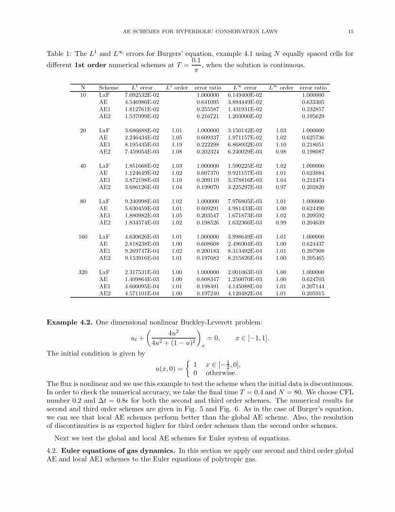
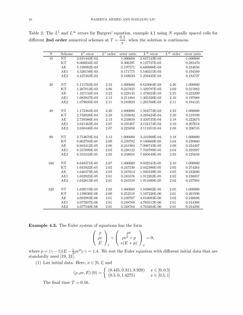
For first order schemes, the numerical errors, the orders of accuracy for the numerical solution,and ratios of the numerical errors of the AE, AE1 and AE2 schemes in comparison with the LxFscheme are shown in Table 1. All the schemes give the required numerical order of accuracy. Wecan see that the local AE2 scheme gives the smallest numerical error followed by the AE1 and AEschemes. The LxF scheme gives the highest L1 and L∞ errors. From Table 2, we can see that forsecond order schemes, local AE2 scheme gives the smallest numerical error followed by the AE1, AEand KT schemes. The NT scheme gives the highest L1 and L∞ errors. But note that as the numberof cells is increased, the AE, AE1, AE2 and KT schemes give nearly the same errors.

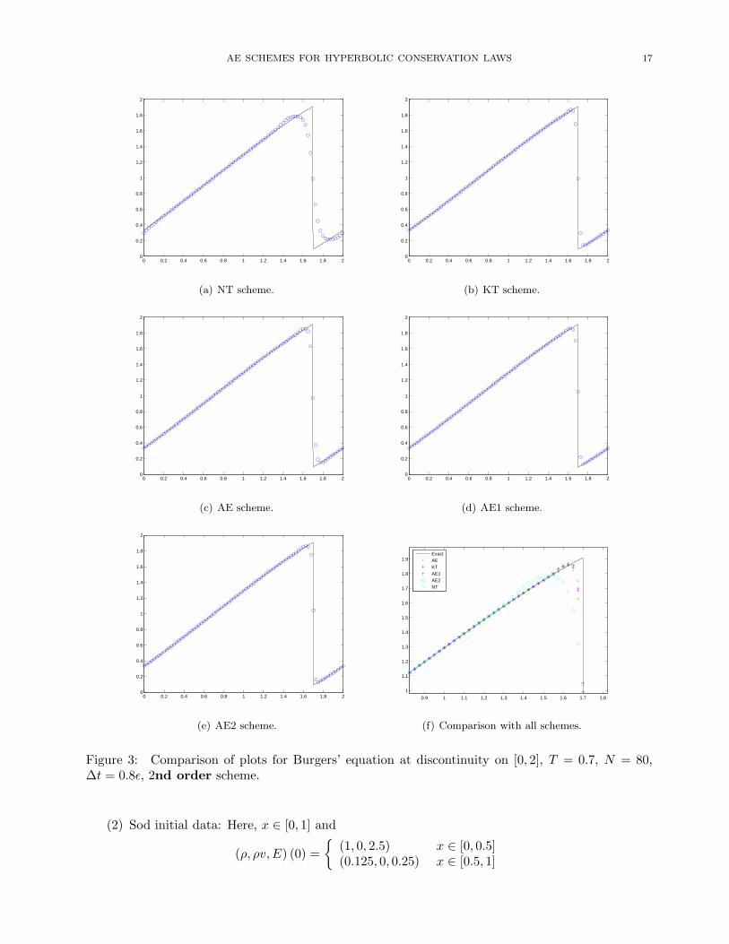
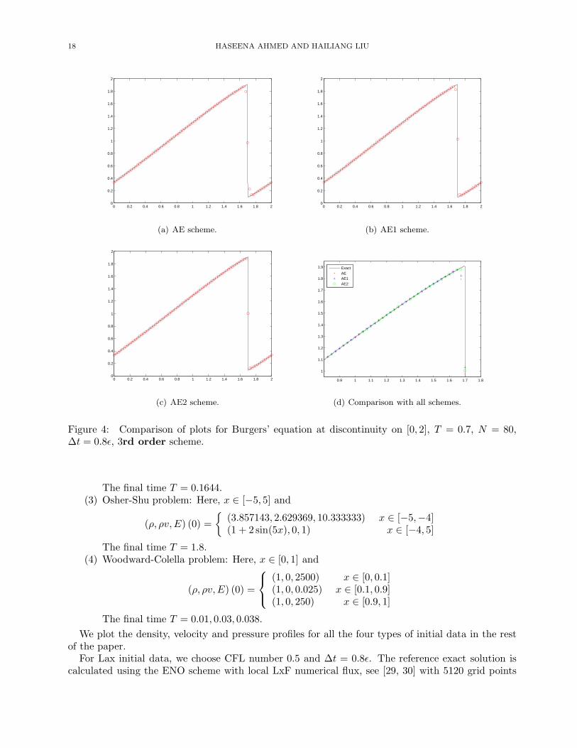
We also plot the solution to the Burgers’ equation when it is discontinuous, that is at time T = 0.7.We use CFL number 0.2 and ∆t = 0.8ǫ for both the second and third order schemes. From Fig. 3and Fig. 4, we see that there is a significant increase in the resolution of discontinuities from secondto third order schemes. We can also see that the local AE schemes perform much better than theglobal AE scheme.


Table 1: The L1 and L∞ errors for Burgers’ equation, example 4.1 using N equally spaced cells for

different 1st order numerical schemes at T =0.1

π, when the solution is continuous.

N Scheme L1 error L1 order error ratio L∞ error L∞ order error ratio

10 LxF 7.092532E-02 1.000000 6.149400E-02 1.000000AE 4.546986E-02 0.641095 3.894449E-02 0.633305AE1 1.812761E-02 0.255587 1.431931E-02 0.232857AE2 1.537099E-02 0.216721 1.203000E-02 0.195629

20 LxF 3.686688E-02 1.01 1.000000 3.150142E-02 1.03 1.000000AE 2.246434E-02 1.05 0.609337 1.971157E-02 1.02 0.625736AE1 8.195435E-03 1.19 0.222298 6.868932E-03 1.10 0.218051AE2 7.459054E-03 1.08 0.202324 6.240029E-03 0.98 0.198087





Example 4.2. One dimensional nonlinear Buckley-Leverett problem:

ut +

(

4u2

4u2 + (1 − u)2

)

x

= 0, x ∈ [−1, 1].

The initial condition is given by

u(x, 0) =

{

1 x ∈ [−12, 0],

0 otherwise.

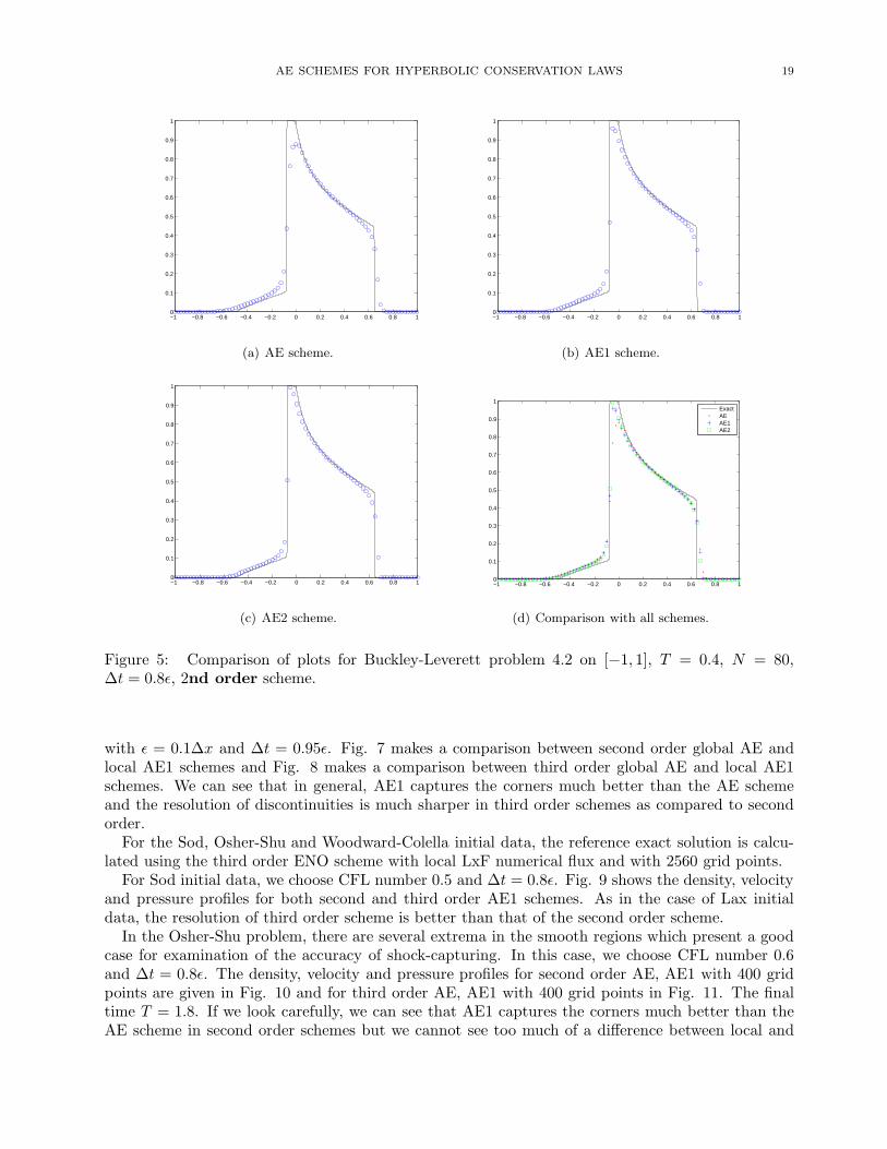
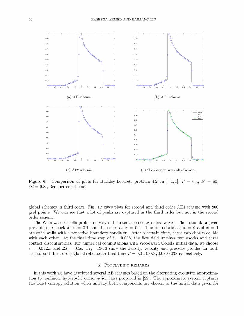
The flux is nonlinear and we use this example to test the scheme when the initial data is discontinuous.In order to check the numerical accuracy, we take the final time T = 0.4 and N = 80. We choose CFLnumber 0.2 and ∆t = 0.8ǫ for both the second and third order schemes. The numerical results forsecond and third order schemes are given in Fig. 5 and Fig. 6. As in the case of Burger’s equation,we can see that local AE schemes perform better than the global AE scheme. Also, the resolutionof discontinuities is as expected higher for third order schemes than the second order schemes.

Next we test the global and local AE schemes for Euler system of equations.

4.2. Euler equations of gas dynamics. In this section we apply our second and third order globalAE and local AE1 schemes to the Euler equations of polytropic gas.


Table 2: The L1 and L∞ errors for Burgers’ equation, example 4.1 using N equally spaced cells for

different 2nd order numerical schemes at T =0.1

π, when the solution is continuous.

N Scheme L1 error L1 order error ratio L∞ error L∞ order error ratio

10 NT 2.631443E-02 1.000000 2.847143E-02 1.000000KT 8.060034E-03 0.306297 8.127727E-03 0.285470AE 5.198982E-03 0.197571 6.680986E-03 0.234656AE1 4.520158E-03 0.171775 5.540215E-03 0.194589AE2 4.437483E-03 0.168633 5.259435E-03 0.184727

20 NT 5.115763E-03 2.53 1.000000 6.623064E-03 2.26 1.000000KT 1.267812E-03 2.86 0.247825 1.429797E-03 2.69 0.215882AE 1.167134E-03 2.23 0.228145 1.478923E-03 2.25 0.223299AE1 1.083947E-03 2.13 0.211884 1.305326E-03 2.16 0.197088AE2 1.079035E-03 2.11 0.210923 1.285700E-03 2.11 0.194125





Example 4.3. The Euler system of equations has the form

ρ

ρv

E

t

+

ρv

ρv2 + p

v(E + p)

x

= 0,

where p = (γ − 1)(E − 12ρv2); γ = 1.4. We test the Euler equation with different initial data that are

standardly used [19, 31].

(1) Lax initial data: Here, x ∈ [0, 1] and

(ρ, ρv,E) (0) =

{

(0.445, 0.311, 8.928) x ∈ [0, 0.5](0.5, 0, 1.4275) x ∈ [0.5, 1]

The final time T = 0.16.


0 0.2 0.4 0.6 0.8 1 1.2 1.4 1.6 1.8 20

0.2

0.4

0.6

0.8

1

1.2

1.4

1.6

1.8

2

(a) NT scheme.

0 0.2 0.4 0.6 0.8 1 1.2 1.4 1.6 1.8 20

0.2

0.4

0.6

0.8

1

1.2

1.4

1.6

1.8

2

(b) KT scheme.

0 0.2 0.4 0.6 0.8 1 1.2 1.4 1.6 1.8 20

0.2

0.4

0.6

0.8

1

1.2

1.4

1.6

1.8

2

(c) AE scheme.

0 0.2 0.4 0.6 0.8 1 1.2 1.4 1.6 1.8 20

0.2

0.4

0.6

0.8

1

1.2

1.4

1.6

1.8

2

(d) AE1 scheme.

0 0.2 0.4 0.6 0.8 1 1.2 1.4 1.6 1.8 20

0.2

0.4

0.6

0.8

1

1.2

1.4

1.6

1.8

2

(e) AE2 scheme.

0.9 1 1.1 1.2 1.3 1.4 1.5 1.6 1.7 1.8

1

1.1

1.2

1.3

1.4

1.5

1.6

1.7

1.8

1.9

ExactAEKTAE1AE2NT

(f) Comparison with all schemes.

Figure 3: Comparison of plots for Burgers’ equation at discontinuity on [0, 2], T = 0.7, N = 80,∆t = 0.8ǫ, 2nd order scheme.

(2) Sod initial data: Here, x ∈ [0, 1] and

(ρ, ρv,E) (0) =

{

(1, 0, 2.5) x ∈ [0, 0.5](0.125, 0, 0.25) x ∈ [0.5, 1]


0 0.2 0.4 0.6 0.8 1 1.2 1.4 1.6 1.8 20

0.2

0.4

0.6

0.8

1

1.2

1.4

1.6

1.8

2

(a) AE scheme.

0 0.2 0.4 0.6 0.8 1 1.2 1.4 1.6 1.8 20

0.2

0.4

0.6

0.8

1

1.2

1.4

1.6

1.8

2

(b) AE1 scheme.

0 0.2 0.4 0.6 0.8 1 1.2 1.4 1.6 1.8 20

0.2

0.4

0.6

0.8

1

1.2

1.4

1.6

1.8

2

(c) AE2 scheme.

0.9 1 1.1 1.2 1.3 1.4 1.5 1.6 1.7 1.8

1

1.1

1.2

1.3

1.4

1.5

1.6

1.7

1.8

1.9

ExactAEAE1AE2

(d) Comparison with all schemes.

Figure 4: Comparison of plots for Burgers’ equation at discontinuity on [0, 2], T = 0.7, N = 80,∆t = 0.8ǫ, 3rd order scheme.

The final time T = 0.1644.(3) Osher-Shu problem: Here, x ∈ [−5, 5] and

(ρ, ρv,E) (0) =

{

(3.857143, 2.629369, 10.333333) x ∈ [−5,−4](1 + 2 sin(5x), 0, 1) x ∈ [−4, 5]

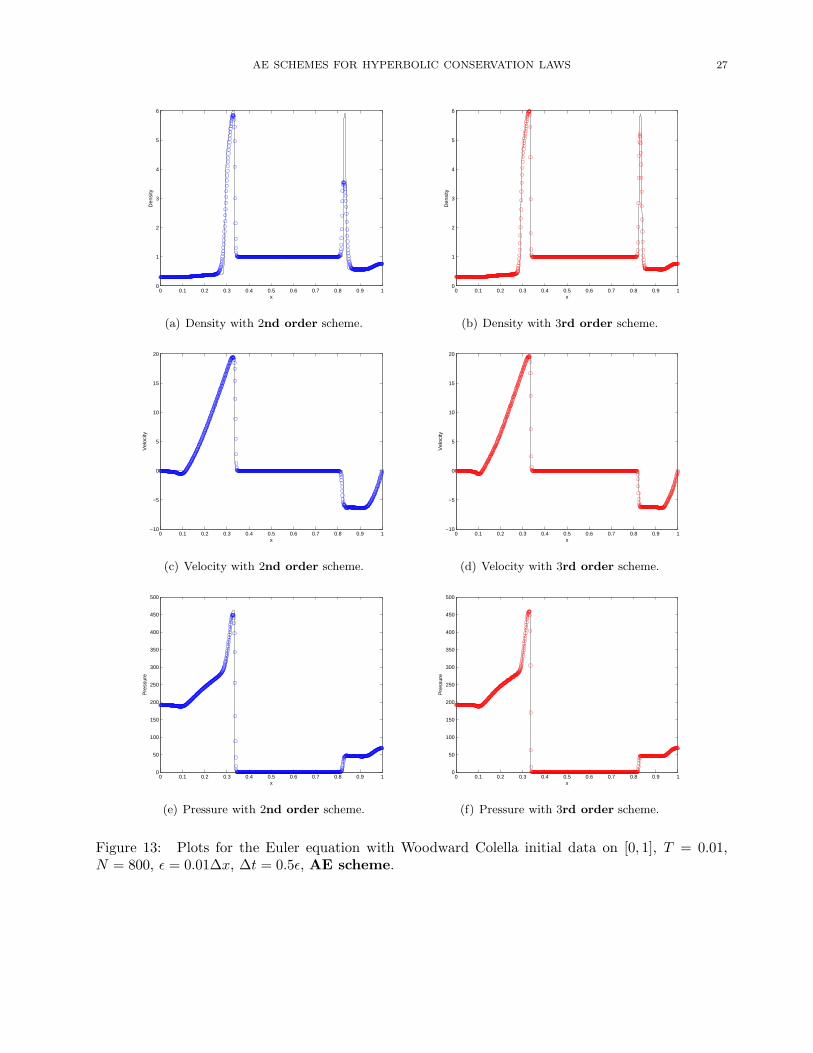
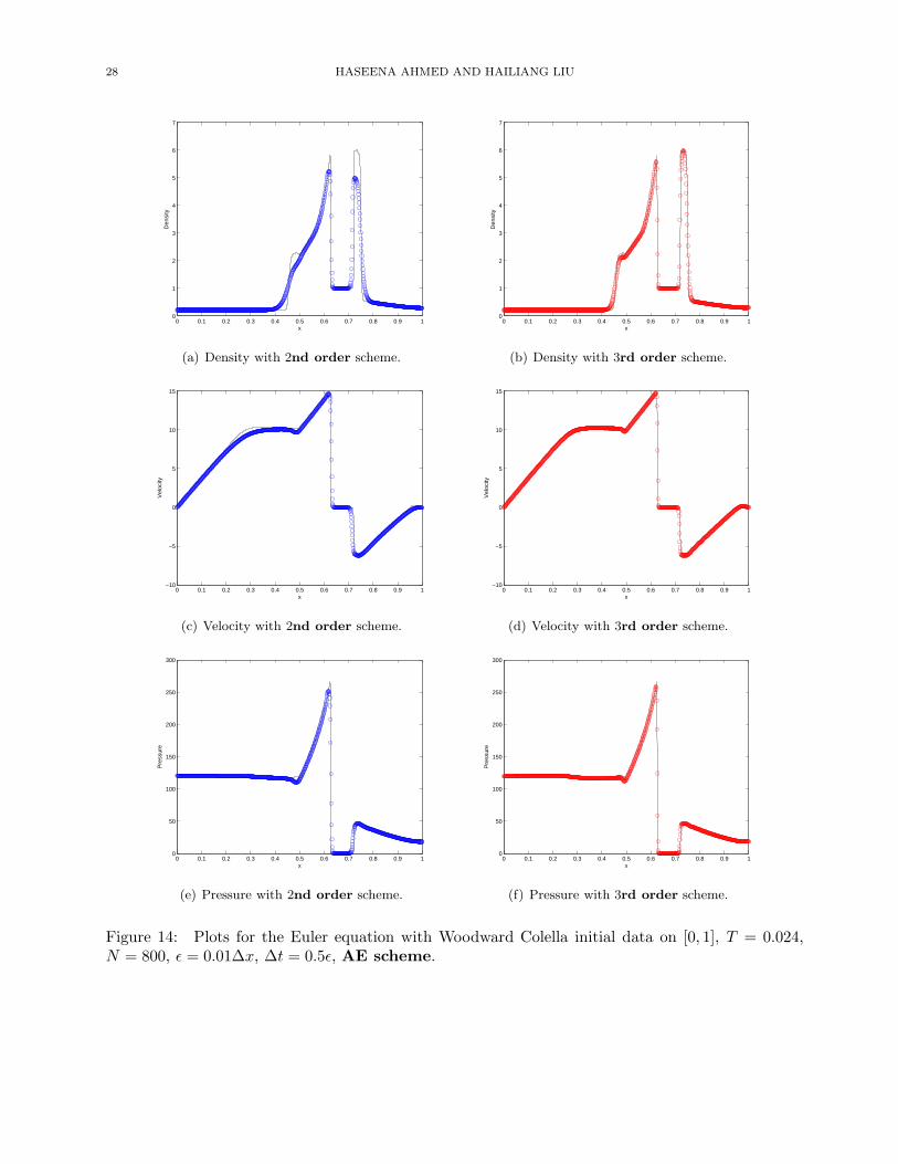
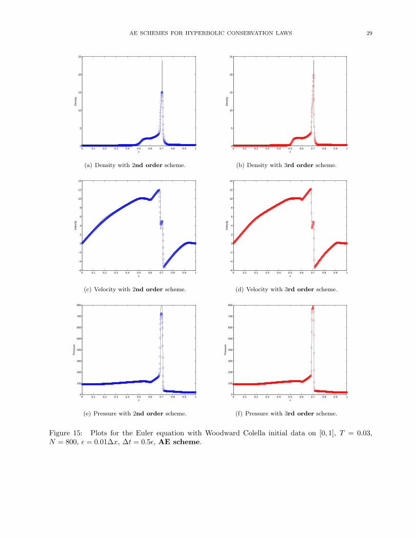
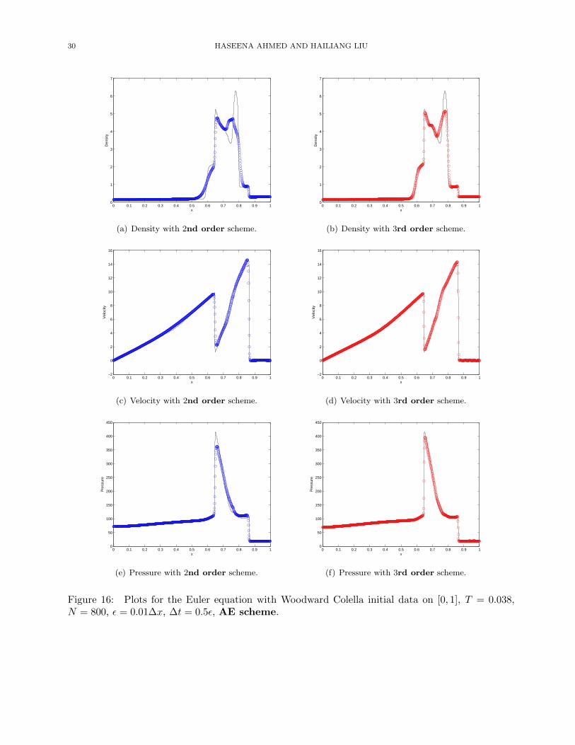
The final time T = 1.8.(4) Woodward-Colella problem: Here, x ∈ [0, 1] and

(ρ, ρv,E) (0) =

(1, 0, 2500) x ∈ [0, 0.1](1, 0, 0.025) x ∈ [0.1, 0.9](1, 0, 250) x ∈ [0.9, 1]

The final time T = 0.01, 0.03, 0.038.

We plot the density, velocity and pressure profiles for all the four types of initial data in the restof the paper.

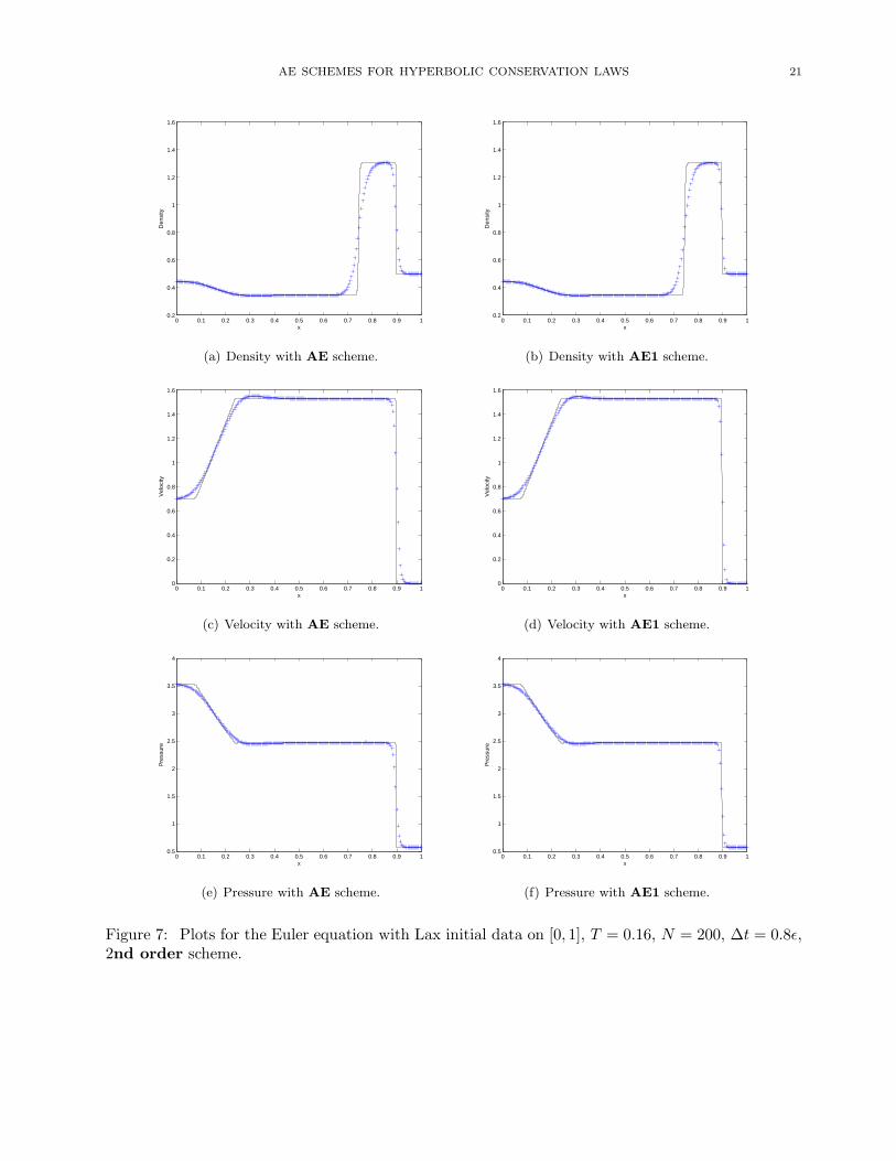
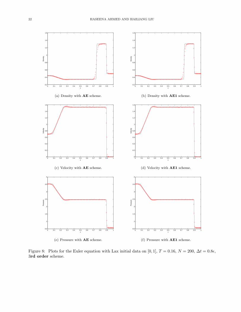
For Lax initial data, we choose CFL number 0.5 and ∆t = 0.8ǫ. The reference exact solution iscalculated using the ENO scheme with local LxF numerical flux, see [29, 30] with 5120 grid points


−1 −0.8 −0.6 −0.4 −0.2 0 0.2 0.4 0.6 0.8 10

0.1

0.2

0.3

0.4

0.5

0.6

0.7

0.8

0.9

1

(a) AE scheme.

−1 −0.8 −0.6 −0.4 −0.2 0 0.2 0.4 0.6 0.8 10

0.1

0.2

0.3

0.4

0.5

0.6

0.7

0.8

0.9

1

(b) AE1 scheme.

−1 −0.8 −0.6 −0.4 −0.2 0 0.2 0.4 0.6 0.8 10

0.1

0.2

0.3

0.4

0.5

0.6

0.7

0.8

0.9

1

(c) AE2 scheme.

−1 −0.8 −0.6 −0.4 −0.2 0 0.2 0.4 0.6 0.8 10

0.1

0.2

0.3

0.4

0.5

0.6

0.7

0.8

0.9

1

ExactAEAE1AE2


Figure 5: Comparison of plots for Buckley-Leverett problem 4.2 on [−1, 1], T = 0.4, N = 80,∆t = 0.8ǫ, 2nd order scheme.

with ǫ = 0.1∆x and ∆t = 0.95ǫ. Fig. 7 makes a comparison between second order global AE andlocal AE1 schemes and Fig. 8 makes a comparison between third order global AE and local AE1schemes. We can see that in general, AE1 captures the corners much better than the AE schemeand the resolution of discontinuities is much sharper in third order schemes as compared to secondorder.

For the Sod, Osher-Shu and Woodward-Colella initial data, the reference exact solution is calcu-lated using the third order ENO scheme with local LxF numerical flux and with 2560 grid points.

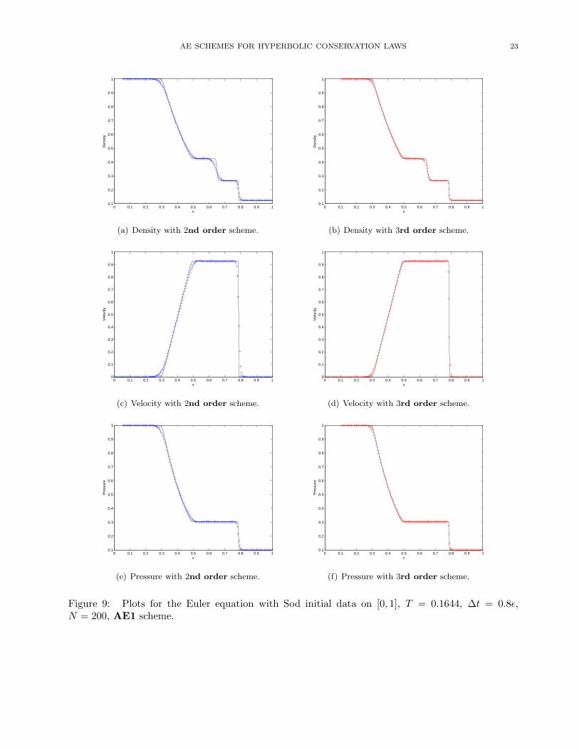
For Sod initial data, we choose CFL number 0.5 and ∆t = 0.8ǫ. Fig. 9 shows the density, velocityand pressure profiles for both second and third order AE1 schemes. As in the case of Lax initialdata, the resolution of third order scheme is better than that of the second order scheme.

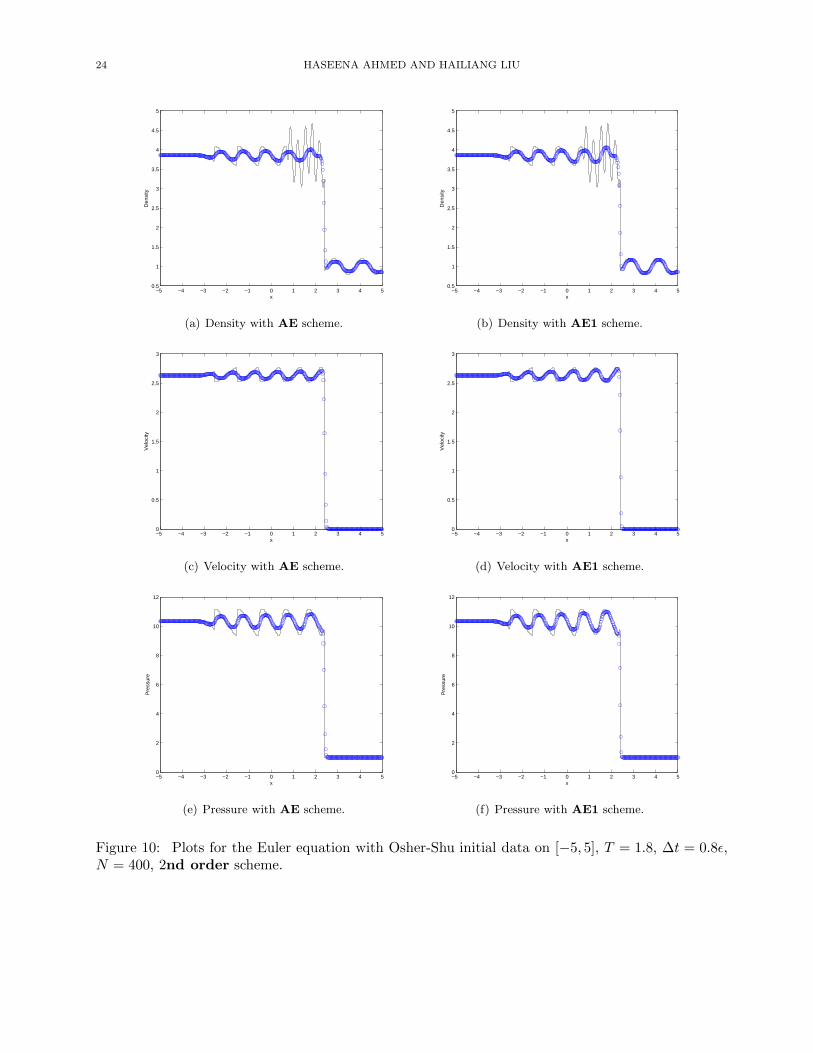
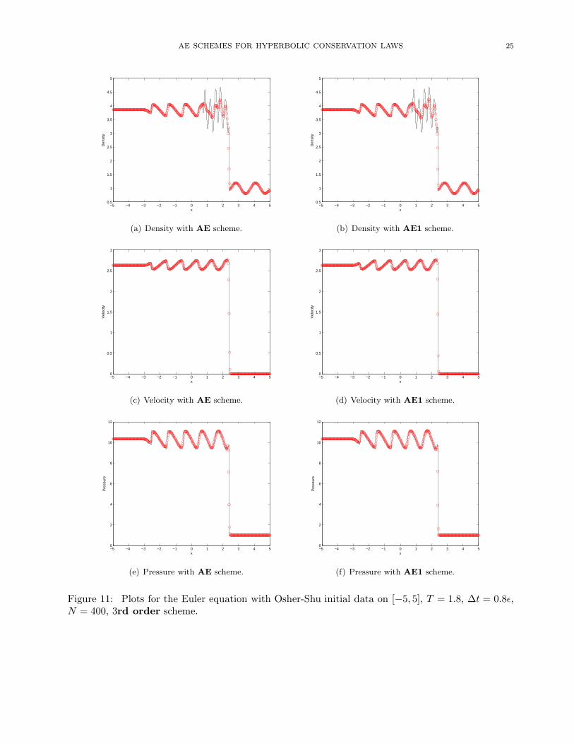
In the Osher-Shu problem, there are several extrema in the smooth regions which present a goodcase for examination of the accuracy of shock-capturing. In this case, we choose CFL number 0.6and ∆t = 0.8ǫ. The density, velocity and pressure profiles for second order AE, AE1 with 400 gridpoints are given in Fig. 10 and for third order AE, AE1 with 400 grid points in Fig. 11. The finaltime T = 1.8. If we look carefully, we can see that AE1 captures the corners much better than theAE scheme in second order schemes but we cannot see too much of a difference between local and


−1 −0.8 −0.6 −0.4 −0.2 0 0.2 0.4 0.6 0.8 10

0.1

0.2

0.3

0.4

0.5

0.6

0.7

0.8

0.9

1

(a) AE scheme.

−1 −0.8 −0.6 −0.4 −0.2 0 0.2 0.4 0.6 0.8 10

0.1

0.2

0.3

0.4

0.5

0.6

0.7

0.8

0.9

1

(b) AE1 scheme.

−1 −0.8 −0.6 −0.4 −0.2 0 0.2 0.4 0.6 0.8 10

0.1

0.2

0.3

0.4

0.5

0.6

0.7

0.8

0.9

1

(c) AE2 scheme.

−1 −0.8 −0.6 −0.4 −0.2 0 0.2 0.4 0.6 0.8 10

0.1

0.2

0.3

0.4

0.5

0.6

0.7

0.8

0.9

1

ExactAEAE1AE2


Figure 6: Comparison of plots for Buckley-Leverett problem 4.2 on [−1, 1], T = 0.4, N = 80,∆t = 0.8ǫ, 3rd order scheme.

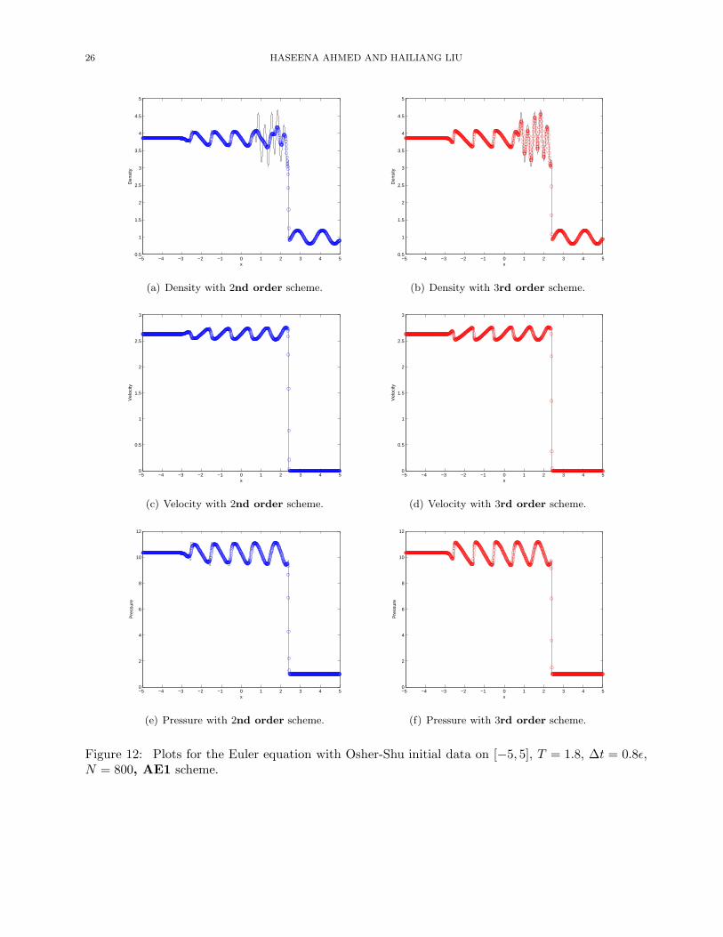
global schemes in third order. Fig. 12 gives plots for second and third order AE1 scheme with 800grid points. We can see that a lot of peaks are captured in the third order but not in the secondorder scheme.

The Woodward-Colella problem involves the interaction of two blast waves. The initial data givenpresents one shock at x = 0.1 and the other at x = 0.9. The boundaries at x = 0 and x = 1are solid walls with a reflective boundary condition. After a certain time, these two shocks collidewith each other. At the final time step of t = 0.038, the flow field involves two shocks and threecontact discontinuities. For numerical computations with Woodward Colella initial data, we chooseǫ = 0.01∆x and ∆t = 0.5ǫ. Fig. 13-16 show the density, velocity and pressure profiles for bothsecond and third order global scheme for final time T = 0.01, 0.024, 0.03, 0.038 respectively.

5. Concluding remarks

In this work we have developed several AE schemes based on the alternating evolution approxima-tion to nonlinear hyperbolic conservation laws proposed in [22]. The approximate system capturesthe exact entropy solution when initially both components are chosen as the initial data given for


0 0.1 0.2 0.3 0.4 0.5 0.6 0.7 0.8 0.9 10.2

0.4

0.6

0.8

1

1.2

1.4

1.6

x

Den

sity

(a) Density with AE scheme.

0 0.1 0.2 0.3 0.4 0.5 0.6 0.7 0.8 0.9 10.2

0.4

0.6

0.8

1

1.2

1.4

1.6

x

Den

sity

(b) Density with AE1 scheme.

0 0.1 0.2 0.3 0.4 0.5 0.6 0.7 0.8 0.9 10

0.2

0.4

0.6

0.8

1

1.2

1.4

1.6

x

Vel

ocity

(c) Velocity with AE scheme.

0 0.1 0.2 0.3 0.4 0.5 0.6 0.7 0.8 0.9 10

0.2

0.4

0.6

0.8

1

1.2

1.4

1.6

x

Vel

ocity

(d) Velocity with AE1 scheme.

0 0.1 0.2 0.3 0.4 0.5 0.6 0.7 0.8 0.9 10.5

1

1.5

2

2.5

3

3.5

4

x

Pre

ssur

e

(e) Pressure with AE scheme.

0 0.1 0.2 0.3 0.4 0.5 0.6 0.7 0.8 0.9 10.5

1

1.5

2

2.5

3

3.5

4

x

Pre

ssur

e

(f) Pressure with AE1 scheme.

Figure 7: Plots for the Euler equation with Lax initial data on [0, 1], T = 0.16, N = 200, ∆t = 0.8ǫ,2nd order scheme.


0 0.1 0.2 0.3 0.4 0.5 0.6 0.7 0.8 0.9 10.2

0.4

0.6

0.8

1

1.2

1.4

1.6

x

Den

sity


0 0.1 0.2 0.3 0.4 0.5 0.6 0.7 0.8 0.9 10.2

0.4

0.6

0.8

1

1.2

1.4

1.6

x

Den

sity


0 0.1 0.2 0.3 0.4 0.5 0.6 0.7 0.8 0.9 10

0.2

0.4

0.6

0.8

1

1.2

1.4

1.6

x

Vel

ocity


0 0.1 0.2 0.3 0.4 0.5 0.6 0.7 0.8 0.9 10

0.2

0.4

0.6

0.8

1

1.2

1.4

1.6

x

Vel

ocity


0 0.1 0.2 0.3 0.4 0.5 0.6 0.7 0.8 0.9 10.5

1

1.5

2

2.5

3

3.5

4

x

Pre

ssur

e


0 0.1 0.2 0.3 0.4 0.5 0.6 0.7 0.8 0.9 10.5

1

1.5

2

2.5

3

3.5

4

x

Pre

ssur

e


Figure 8: Plots for the Euler equation with Lax initial data on [0, 1], T = 0.16, N = 200, ∆t = 0.8ǫ,3rd order scheme.


0 0.1 0.2 0.3 0.4 0.5 0.6 0.7 0.8 0.9 10.1

0.2

0.3

0.4

0.5

0.6

0.7

0.8

0.9

1

x

Den

sity

(a) Density with 2nd order scheme.

0 0.1 0.2 0.3 0.4 0.5 0.6 0.7 0.8 0.9 10.1

0.2

0.3

0.4

0.5

0.6

0.7

0.8

0.9

1

x

Den

sity

(b) Density with 3rd order scheme.

0 0.1 0.2 0.3 0.4 0.5 0.6 0.7 0.8 0.9 10

0.1

0.2

0.3

0.4

0.5

0.6

0.7

0.8

0.9

1

x

Vel

ocity

(c) Velocity with 2nd order scheme.

0 0.1 0.2 0.3 0.4 0.5 0.6 0.7 0.8 0.9 10

0.1

0.2

0.3

0.4

0.5

0.6

0.7

0.8

0.9

1

x

Vel

ocity

(d) Velocity with 3rd order scheme.

0 0.1 0.2 0.3 0.4 0.5 0.6 0.7 0.8 0.9 10.1

0.2

0.3

0.4

0.5

0.6

0.7

0.8

0.9

1

x

Pre

ssur

e

(e) Pressure with 2nd order scheme.

0 0.1 0.2 0.3 0.4 0.5 0.6 0.7 0.8 0.9 10.1

0.2

0.3

0.4

0.5

0.6

0.7

0.8

0.9

1

x

Pre

ssur

e

(f) Pressure with 3rd order scheme.

Figure 9: Plots for the Euler equation with Sod initial data on [0, 1], T = 0.1644, ∆t = 0.8ǫ,N = 200, AE1 scheme.


−5 −4 −3 −2 −1 0 1 2 3 4 50.5

1

1.5

2

2.5

3

3.5

4

4.5

5

x

Den

sity


−5 −4 −3 −2 −1 0 1 2 3 4 50.5

1

1.5

2

2.5

3

3.5

4

4.5

5

x

Den

sity


−5 −4 −3 −2 −1 0 1 2 3 4 50

0.5

1

1.5

2

2.5

3

x

Vel

ocity


−5 −4 −3 −2 −1 0 1 2 3 4 50

0.5

1

1.5

2

2.5

3

x

Vel

ocity


−5 −4 −3 −2 −1 0 1 2 3 4 50

2

4

6

8

10

12

x

Pre

ssur

e


−5 −4 −3 −2 −1 0 1 2 3 4 50

2

4

6

8

10

12

x

Pre

ssur

e


Figure 10: Plots for the Euler equation with Osher-Shu initial data on [−5, 5], T = 1.8, ∆t = 0.8ǫ,N = 400, 2nd order scheme.


−5 −4 −3 −2 −1 0 1 2 3 4 50.5

1

1.5

2

2.5

3

3.5

4

4.5

5

x

Den

sity


−5 −4 −3 −2 −1 0 1 2 3 4 50.5

1

1.5

2

2.5

3

3.5

4

4.5

5

x

Den

sity


−5 −4 −3 −2 −1 0 1 2 3 4 50

0.5

1

1.5

2

2.5

3

x

Vel

ocity


−5 −4 −3 −2 −1 0 1 2 3 4 50

0.5

1

1.5

2

2.5

3

x

Vel

ocity


−5 −4 −3 −2 −1 0 1 2 3 4 50

2

4

6

8

10

12

x

Pre

ssur

e


−5 −4 −3 −2 −1 0 1 2 3 4 50

2

4

6

8

10

12

x

Pre

ssur

e


Figure 11: Plots for the Euler equation with Osher-Shu initial data on [−5, 5], T = 1.8, ∆t = 0.8ǫ,N = 400, 3rd order scheme.


−5 −4 −3 −2 −1 0 1 2 3 4 50.5

1

1.5

2

2.5

3

3.5

4

4.5

5

x

Den

sity


−5 −4 −3 −2 −1 0 1 2 3 4 50.5

1

1.5

2

2.5

3

3.5

4

4.5

5

x

Den

sity


−5 −4 −3 −2 −1 0 1 2 3 4 50

0.5

1

1.5

2

2.5

3

x

Vel

ocity


−5 −4 −3 −2 −1 0 1 2 3 4 50

0.5

1

1.5

2

2.5

3

x

Vel

ocity


−5 −4 −3 −2 −1 0 1 2 3 4 50

2

4

6

8

10

12

x

Pre

ssur

e


−5 −4 −3 −2 −1 0 1 2 3 4 50

2

4

6

8

10

12

x

Pre

ssur

e


Figure 12: Plots for the Euler equation with Osher-Shu initial data on [−5, 5], T = 1.8, ∆t = 0.8ǫ,N = 800, AE1 scheme.


0 0.1 0.2 0.3 0.4 0.5 0.6 0.7 0.8 0.9 10

1

2

3

4

5

6

x

Den

sity


0 0.1 0.2 0.3 0.4 0.5 0.6 0.7 0.8 0.9 10

1

2

3

4

5

6

x

Den

sity


0 0.1 0.2 0.3 0.4 0.5 0.6 0.7 0.8 0.9 1−10

−5

0

5

10

15

20

x

Vel

ocity


0 0.1 0.2 0.3 0.4 0.5 0.6 0.7 0.8 0.9 1−10

−5

0

5

10

15

20

x

Vel

ocity


0 0.1 0.2 0.3 0.4 0.5 0.6 0.7 0.8 0.9 10

50

100

150

200

250

300

350

400

450

500

x

Pre

ssur

e


0 0.1 0.2 0.3 0.4 0.5 0.6 0.7 0.8 0.9 10

50

100

150

200

250

300

350

400

450

500

x

Pre

ssur

e


Figure 13: Plots for the Euler equation with Woodward Colella initial data on [0, 1], T = 0.01,N = 800, ǫ = 0.01∆x, ∆t = 0.5ǫ, AE scheme.


0 0.1 0.2 0.3 0.4 0.5 0.6 0.7 0.8 0.9 10

1

2

3

4

5

6

7

x

Den

sity


0 0.1 0.2 0.3 0.4 0.5 0.6 0.7 0.8 0.9 10

1

2

3

4

5

6

7

x

Den

sity


0 0.1 0.2 0.3 0.4 0.5 0.6 0.7 0.8 0.9 1−10

−5

0

5

10

15

x

Vel

ocity


0 0.1 0.2 0.3 0.4 0.5 0.6 0.7 0.8 0.9 1−10

−5

0

5

10

15

x

Vel

ocity


0 0.1 0.2 0.3 0.4 0.5 0.6 0.7 0.8 0.9 10

50

100

150

200

250

300

x

Pre

ssur

e


0 0.1 0.2 0.3 0.4 0.5 0.6 0.7 0.8 0.9 10

50

100

150

200

250

300

x

Pre

ssur

e




0 0.1 0.2 0.3 0.4 0.5 0.6 0.7 0.8 0.9 10

5

10

15

20

25

x

Den

sity


0 0.1 0.2 0.3 0.4 0.5 0.6 0.7 0.8 0.9 10

5

10

15

20

25

x

Den

sity


0 0.1 0.2 0.3 0.4 0.5 0.6 0.7 0.8 0.9 1−6

−4

−2

0

2

4

6

8

10

12

14

x

Vel

ocity


0 0.1 0.2 0.3 0.4 0.5 0.6 0.7 0.8 0.9 1−6

−4

−2

0

2

4

6

8

10

12

14

x

Vel

ocity


0 0.1 0.2 0.3 0.4 0.5 0.6 0.7 0.8 0.9 10

100

200

300

400

500

600

700

800

x

Pre

ssur

e


0 0.1 0.2 0.3 0.4 0.5 0.6 0.7 0.8 0.9 10

100

200

300

400

500

600

700

800

x

Pre

ssur

e




0 0.1 0.2 0.3 0.4 0.5 0.6 0.7 0.8 0.9 10

1

2

3

4

5

6

7

x

Den

sity


0 0.1 0.2 0.3 0.4 0.5 0.6 0.7 0.8 0.9 10

1

2

3

4

5

6

7

x

Den

sity


0 0.1 0.2 0.3 0.4 0.5 0.6 0.7 0.8 0.9 1−2

0

2

4

6

8

10

12

14

16

x

Vel

ocity


0 0.1 0.2 0.3 0.4 0.5 0.6 0.7 0.8 0.9 1−2

0

2

4

6

8

10

12

14

16

x

Vel

ocity


0 0.1 0.2 0.3 0.4 0.5 0.6 0.7 0.8 0.9 10

50

100

150

200

250

300

350

400

450

x

Pre

ssur

e


0 0.1 0.2 0.3 0.4 0.5 0.6 0.7 0.8 0.9 10

50

100

150

200

250

300

350

400

450

x

Pre

ssur

e




the conservation laws. Such a feature allows for a sampling of two components over alternatinggrids. High order accuracy in space is further achieved by the piece-wise polynomial reconstructionfrom averages of two components, respectively. Time discretization is via the standard Runge-Kuttamethod. Local AE schemes are made possible by letting the scale parameter ǫ reflect the localdistribution of nonlinear waves. The AE schemes have the advantage of easier formulation and im-plementation, and efficient computation of the solution. For the first and second order local AEschemes applied to scalar laws, we have proved both the maximum principle and total variationdiminishing (TVD) property. Numerical tests for both scalar conservation laws and compressibleEuler equations presented in this work have demonstrated the high order accuracy and capacity ofthese AE schemes. Extension to multi-dimensional problems is straightforward.

Acknowledgments

This research was supported by the National Science Foundation under Grant DMS05-05975.

References

[1] R. Artebrant and H. J. Schroll. Conservative logarithmic reconstructions and finite volume methods. SIAM J. Sci.Comput., 27(1):294–314 (electronic), 2005.

[2] F. Bianco, G. Puppo, and G. Russo. High-order central schemes for hyperbolic systems of conservation laws. SIAMJ. Sci. Comput., 21(1):294–322 (electronic), 1999.

[3] B. Cockburn and C.-W. Shu. Runge-Kutta discontinuous Galerkin methods for convection-dominated problems.J. Sci. Comput., 16(3):173–261, 2001.

[4] P. Colella and P. R. Woodward. The piecewise parabolic method (ppm) for gas-dynamical simulations. J. Comput.Phys., 54(1):174–201, 1984.

[5] B. Engquist and S. Osher. One-sided difference approximations for nonlinear conservation laws. Math. Comp.,36(154):321–351, 1981.

[6] K. O. Friedrichs. Symmetric hyperbolic linear differential equations. Comm. Pure Appl. Math., 7:345–392, 1954.[7] S. K. Godunov. A difference method for numerical calculation of discontinuous solutions of the equations of

hydrodynamics. Mat. Sb. (N.S.), 47 (89):271–306, 1959.[8] A. Harten. High resolution schemes for hyperbolic conservation laws. J. Comput. Phys., 49(3):357–393, 1983.[9] A. Harten, B. Engquist, S. Osher, and S. R. Chakravarthy. Uniformly high-order accurate essentially nonoscillatory

schemes. III. J. Comput. Phys., 71(2):231–303, 1987.[10] A. Harten, P. D. Lax, and B. van Leer. On upstream differencing and Godunov-type schemes for hyperbolic

conservation laws. SIAM Rev., 25(1):35–61, 1983.[11] G.-S. Jiang and E. Tadmor. Nonoscillatory central schemes for multidimensional hyperbolic conservation laws.

SIAM J. Sci. Comput., 19(6):1892–1917 (electronic), 1998.[12] S. Jin and Z. P. Xin. The relaxation schemes for systems of conservation laws in arbitrary space dimensions.

Comm. Pure Appl. Math., 48(3):235–276, 1995.[13] M. A. Katsoulakis and A. E. Tzavaras. Contractive relaxation systems and the scalar multidimensional conservation

law. Comm. Partial Differential Equations, 22(1-2):195–233, 1997.[14] S. N. Kruzkov. First order quasilinear equations with several independent variables. Mat. Sb. (N.S.), 81 (123):228–

255, 1970.[15] A. Kurganov, S. Noelle, and G. Petrova. Semidiscrete central-upwind schemes for hyperbolic conservation laws

and Hamilton-Jacobi equations. SIAM J. Sci. Comput., 23(3):707–740 (electronic), 2001.[16] A. Kurganov and G. Petrova. A third-order semi-discrete genuinely multidimensional central scheme for hyperbolic

conservation laws and related problems. Numer. Math., 88(4):683–729, 2001.[17] A. Kurganov and E. Tadmor. New high-resolution central schemes for nonlinear conservation laws and convection-

diffusion equations. J. Comput. Phys., 160(1):241–282, 2000.[18] P. D. Lax. Weak solutions of nonlinear hyperbolic equations and their numerical computation. Comm. Pure Appl.

Math., 7:159–193, 1954.[19] R. J. LeVeque. Numerical methods for conservation laws. Lectures in Mathematics ETH Zurich. Birkhauser Verlag,

Basel, second edition, 1992.[20] D. Levy, G. Puppo, and G. Russo. Central WENO schemes for hyperbolic systems of conservation laws. M2AN

Math. Model. Numer. Anal., 33(3):547–571, 1999.


[21] P.-L. Lions, B. Perthame, and E. Tadmor. A kinetic formulation of multidimensional scalar conservation laws andrelated equations. J. Amer. Math. Soc., 7(1):169–191, 1994.

[22] H. Liu. An alternating evolution approximation to systems of hyperbolic conservation laws. J. Hyperbolic Differ.Equ. to appear.

[23] X.-D. Liu, S. Osher, and T. Chan. Weighted essentially non-oscillatory schemes. J. Comput. Phys., 115(1):200–212,1994.

[24] X.-D. Liu and E. Tadmor. Third order nonoscillatory central scheme for hyperbolic conservation laws. Numer.Math., 79(3):397–425, 1998.

[25] Y. Liu. Central schemes on overlapping cells. J. Comput. Phys., 209(1):82–104, 2005.[26] R. Natalini. A discrete kinetic approximation of entropy solutions to multidimensional scalar conservation laws.

J. Differential Equations, 148(2):292–317, 1998.[27] H. Nessyahu and E. Tadmor. Nonoscillatory central differencing for hyperbolic conservation laws. J. Comput.

Phys., 87(2):408–463, 1990.[28] B. Perthame and E. Tadmor. A kinetic equation with kinetic entropy functions for scalar conservation laws. Comm.

Math. Phys., 136(3):501–517, 1991.[29] C.-W. Shu and S. Osher. Efficient implementation of essentially nonoscillatory shock-capturing schemes. J. Comput.

Phys., 77(2):439–471, 1988.[30] C.-W. Shu and S. Osher. Efficient implementation of essentially nonoscillatory shock-capturing schemes. II. J.

Comput. Phys., 83(1):32–78, 1989.[31] E. F. Toro. Riemann solvers and numerical methods for fluid dynamics. Springer-Verlag, Berlin, second edition,

1999. A practical introduction.[32] B. van Leer. Upwind differencing for hyperbolic systems of conservation laws. In Numerical methods for engineering,

1 (Paris, 1980), pages 137–149. Dunod, Paris, 1980.[33] B. van Leer. Towards the ultimate conservative difference scheme. V. A second-order sequel to Godunov’s method

[J. Comput. Phys. 32 (1979), no. 1, 101–136]. J. Comput. Phys., 135(2):227–248, 1997. With an introduction byCh. Hirsch, Commemoration of the 30th anniversary {of J. Comput. Phys.}.

[34] Z. Wang. Spectral volume method for conservation laws on unstructured grids: basic formulation. J. Comp. Phys.,178:210–251, 2002.

Iowa State University, Mathematics Department, Ames, IA 50011

E-mail address: [email protected]; [email protected]

FORMULATION AND ANALYSIS OF ALTERNATING EVOLUTION (AE) SCHEMES

Documents

Transcript of FORMULATION AND ANALYSIS OF ALTERNATING EVOLUTION (AE) SCHEMES