1

Review of Probability (for Lossless Section)

For Details See:

Appendix A in text book

Ch. 10 in Lathi’s Book

2

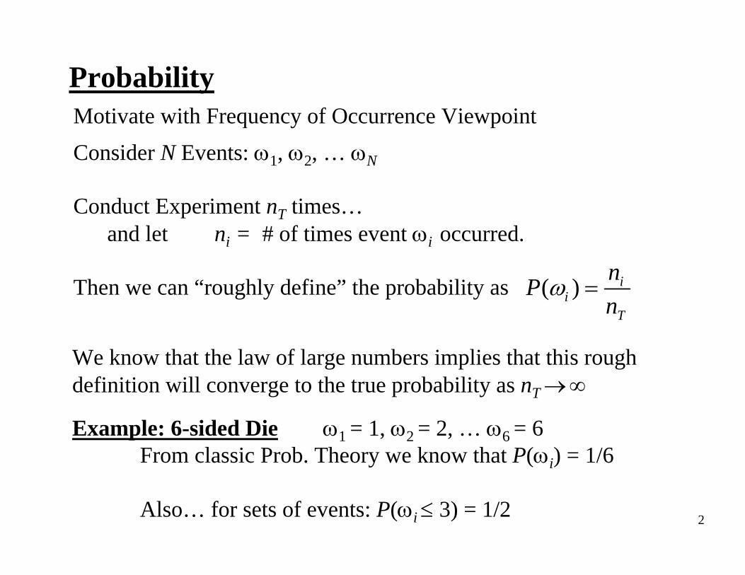
Motivate with Frequency of Occurrence ViewpointConsider N Events: ω1, ω2, … ωN

Conduct Experiment nT times…and let ni = # of times event ωi occurred.

Then we can “roughly define” the probability as

Probability

( ) ii

T

nPn

ω =

We know that the law of large numbers implies that this rough definition will converge to the true probability as nT→∞

Example: 6-sided Die ω1 = 1, ω2 = 2, … ω6 = 6From classic Prob. Theory we know that P(ωi) = 1/6

Also… for sets of events: P(ωi ≤ 3) = 1/2

3

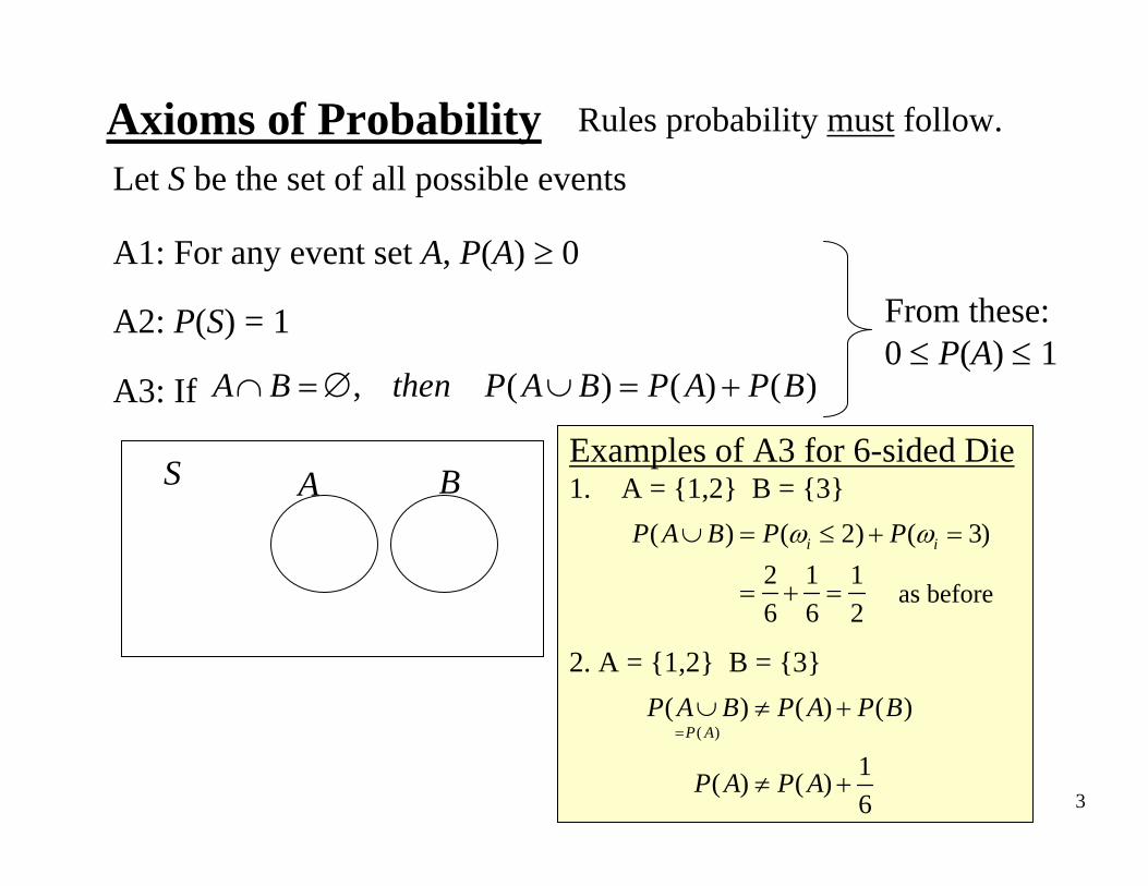
Let S be the set of all possible events

A1: For any event set A, P(A) ≥ 0

A2: P(S) = 1

A3: If

Axioms of Probability

, ( ) ( ) ( )A B then P A B P A P B∩ =∅ ∪ = +

S A B

From these: 0 ≤ P(A) ≤ 1

Rules probability must follow.

Examples of A3 for 6-sided Die1. A = {1,2} B = {3}

2. A = {1,2} B = {3}

( ) ( 2) ( 3)2 1 16 6 2

i iP A B P Pω ω∪ = ≤ + =

= + = as before

( )( ) ( ) ( )

1( ) ( )6

P AP A B P A P B

P A P A

=∪ ≠ +

≠ +

4

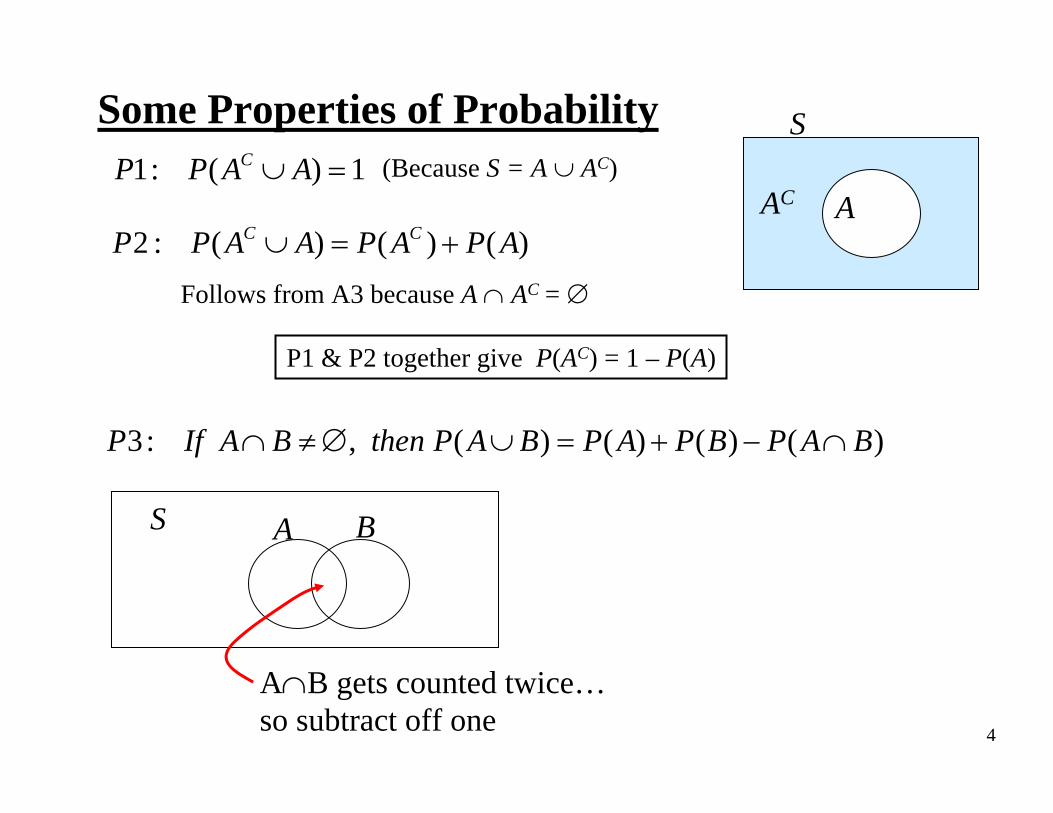
Some Properties of Probability1: ( ) 1CP P A A∪ =

2 : ( ) ( ) ( )C CP P A A P A P A∪ = +

3: , ( ) ( ) ( ) ( )P If A B then P A B P A P B P A B∩ ≠∅ ∪ = + − ∩

S A B

A∩B gets counted twice…so subtract off one

S

AAC(Because S = A ∪ AC)

Follows from A3 because A ∩ AC = ∅

P1 & P2 together give P(AC) = 1 – P(A)

5

Joint ProbabilityConsider two separate “experiments”: The probability that… the 1st experiment had outcome A

…AND… the 2nd experiment had outcome B

is denoted as P(A,B)

Often A & B come from a single experiment having multiple observations…

Experiment: Randomly choose a personObservations: Height & Weight of chosen person

P(H > 6’ , W > 170 lbs) = prob the selected person is taller than 6’AND weighs more than 170 lbs

6

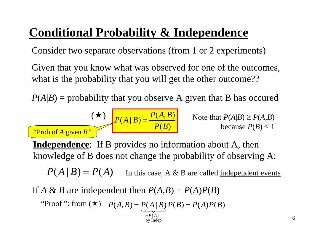
Conditional Probability & IndependenceConsider two separate observations (from 1 or 2 experiments)

Given that you know what was observed for one of the outcomes, what is the probability that you will get the other outcome??

P(A|B) = probability that you observe A given that B has occured

( , )( | )( )

P A BP A BP B

= Note that P(A|B) ≥ P(A,B) because P(B) ≤ 1

“Prob of A given B”

Independence: If B provides no information about A, then knowledge of B does not change the probability of observing A:

( | ) ( )P A B P A= In this case, A & B are called independent events

If A & B are independent then P(A,B) = P(A)P(B)“Proof ”: from ( )

( )by Indep

( , ) ( | ) ( ) ( ) ( )P A

P A B P A B P B P A P B=

= =

( )

7

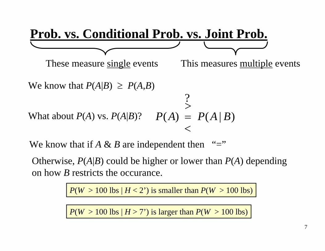
Prob. vs. Conditional Prob. vs. Joint Prob.

These measure single events This measures multiple events

We know that P(A|B) ≥ P(A,B)

What about P(A) vs. P(A|B)?

?( ) ( | )P A P A B

>=<

We know that if A & B are independent then “=”

Otherwise, P(A|B) could be higher or lower than P(A) depending on how B restricts the occurance.

P(W > 100 lbs | H < 2’) is smaller than P(W > 100 lbs)

P(W > 100 lbs | H > 7’) is larger than P(W > 100 lbs)

8

Example: Prob of Characters in English Text1. What is the prob. of getting a specific letter?

Most probable letter is e: P(e) ≈ 0.127

q and z are least probable: P(q) ≈ P(z) ≈ 0.001

2. If you know the current letter… What is the prob. of getting a specific letter in the next position?

Say current letter is q:

P(u|q) ≈ 0.99 P(e|q) ≈ 0.001

Just Guesses!Just Guesses!

Note: P(e|q) < P(e) prior info decreases probP(u|q) > P(u) prior info increases prob

Knowing the current letter completely redistributes the probability of the next letter (i.e., sequential letters are not independent)

9

Random Variables (RVs)Mathematical tool to assign #’s to events

Note: a problem may provide a natural assignment

To each outcome ωi assign a number X(ωi)

Examples: • ASCII code for symbols

• Letter grades get mapped to {0, 1, 2, 3, 4}

Purpose: to allow numerical analyses such as…• Plots…• Sums (means, variances)…• Sets define via inequalities…• Prob. Functions…• Etc.

10

Discrete RVsFor now we will limit ourselves to Discrete RVs

(Later for lossy compression we will need Continuous RVs)

A Discrete RV X can take on values only from• A finite set• A countably infinite set (e.g., the integers but not the reals)

The finite-set case is the more important one here

Examples• X can take only values in the set {0, 0.5, 1, 1.5, … , 9.5, 10}• X can take only values in the set {0, 1, 2, 3, … }• An RV X that can take any value in the interval [0, 1] is NOT discrete; it is continuous

11

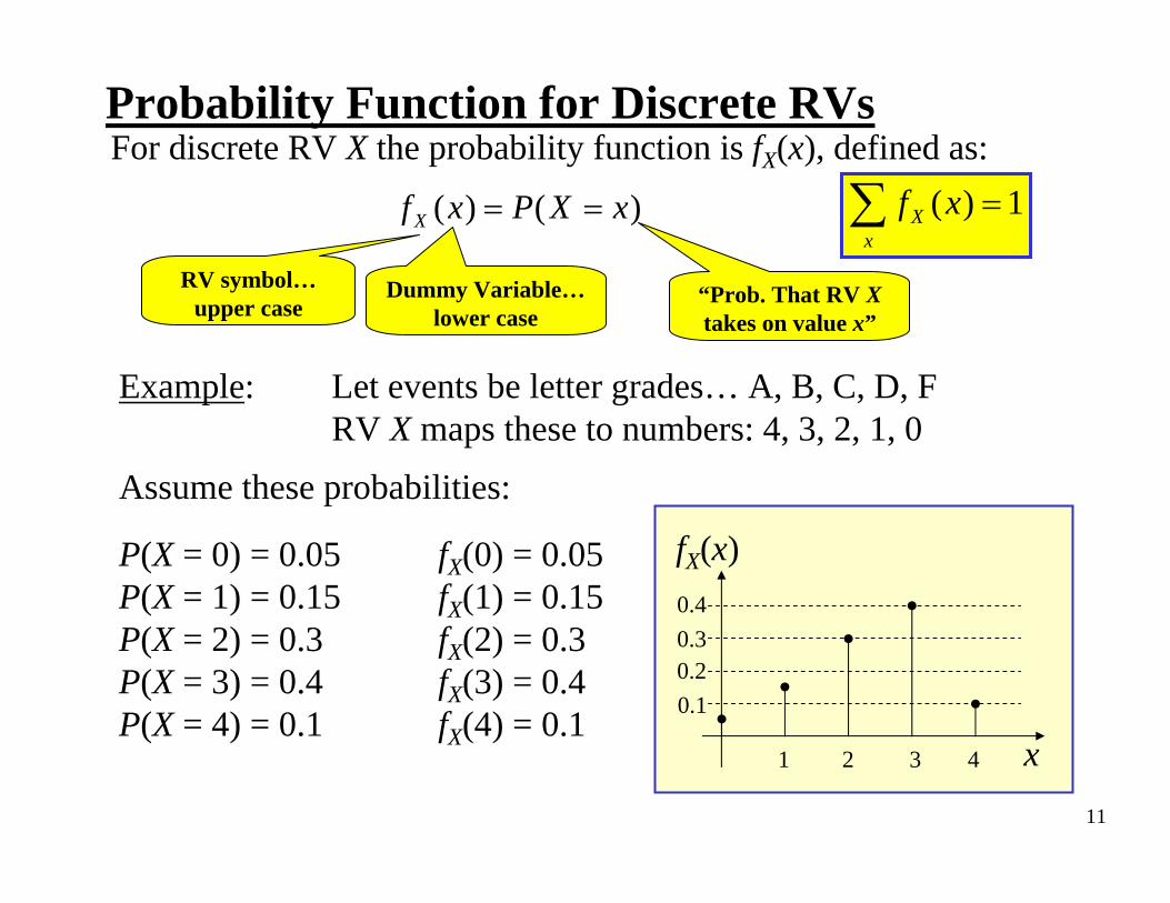
Probability Function for Discrete RVsFor discrete RV X the probability function is fX(x), defined as:

( ) ( )Xf x P X x= =

RV symbol…upper case

Dummy Variable…lower case

“Prob. That RV Xtakes on value x”

Example: Let events be letter grades… A, B, C, D, FRV X maps these to numbers: 4, 3, 2, 1, 0

Assume these probabilities:

P(X = 0) = 0.05 fX(0) = 0.05P(X = 1) = 0.15 fX(1) = 0.15P(X = 2) = 0.3 fX(2) = 0.3P(X = 3) = 0.4 fX(3) = 0.4P(X = 4) = 0.1 fX(4) = 0.1

( ) 1Xx

f x =∑

x

fX(x)

0.20.1

0.30.4

1 2 3 4

12

x

FX(x)

0.20.1

0.30.4

1 2 3 4

0.50.60.70.80.91.0

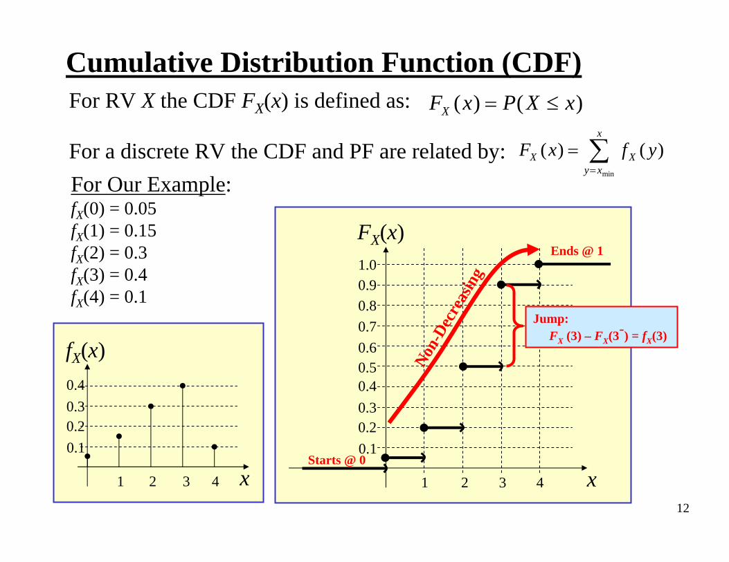
Cumulative Distribution Function (CDF)For RV X the CDF FX(x) is defined as: ( ) ( )XF x P X x= ≤

For Our Example: fX(0) = 0.05fX(1) = 0.15fX(2) = 0.3fX(3) = 0.4fX(4) = 0.1

min

( ) ( )x

X Xy x

F x f y=

= ∑For a discrete RV the CDF and PF are related by:

x

fX(x)

0.20.1

0.30.4

1 2 3 4

Non-D

ecre

asin

gStarts @ 0

Ends @ 1

Jump: FX (3) – FX(3-) = fX(3)

13

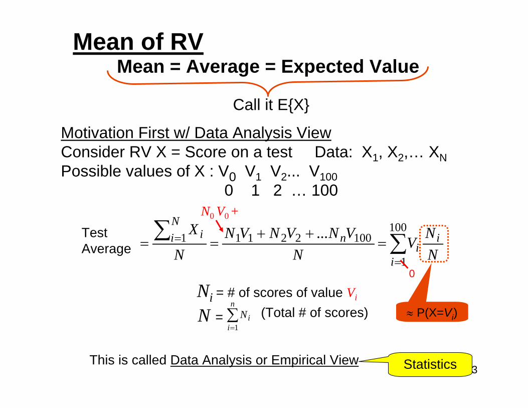
Motivation First w/ Data Analysis ViewConsider RV X = Score on a test Data: X1, X2,… XNPossible values of X : V0 V1 V2... V100

0 1 2 … 100

This is called Data Analysis or Empirical View

Mean of RVMean = Average = Expected Value

Call it E{X}

Test Average

≈ P(X=Vi)

∑∑=

= =++

==100

1

10022111 ...

i

ii

nNi i

NNV

NVNVNVN

N

X

Ni = # of scores of value Vi

N = (Total # of scores)∑=

n

iiN

1

Statistics

0

N0 V0 +

14

Theoretical View of Mean

For Discrete random Variables :

Data Analysis View leads to Probability Theory:

1

{ } ( )n

i X in

X x f x=

Ε = ∑Probability

Notation: { } XX X mΕ = =

{ } { }E aX b aE X b+ = +Property:

where X is an RV and a and b are just numbers

15

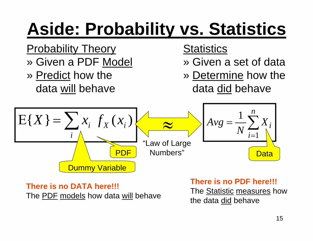
Aside: Probability vs. StatisticsProbability Theory» Given a PDF Model» Predict how the

data will behave

Statistics» Given a set of data» Determine how the

data did behave

∑=

=n

iiX

NAvg

1

1

Data

There is no DATA here!!!The PDF models how data will behave

There is no PDF here!!!The Statistic measures how the data did behave

{ } ( )i X ii

X x f xΕ =∑

Dummy Variable

PDF

≈“Law of Large

Numbers”

16

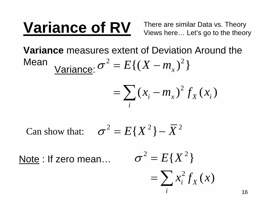
Variance of RVVariance measures extent of Deviation Around the Mean

There are similar Data vs. Theory Views here… Let’s go to the theory

Variance: 2 2

2

{( ) }

( ) ( )

x

i x X ii

E X m

x m f x

σ = −

= −∑

Note : If zero mean… 2 2

2

{ }( )i X

i

E Xx f x

σ =

=∑

2 2 2{ }E X Xσ = −Can show that:

17

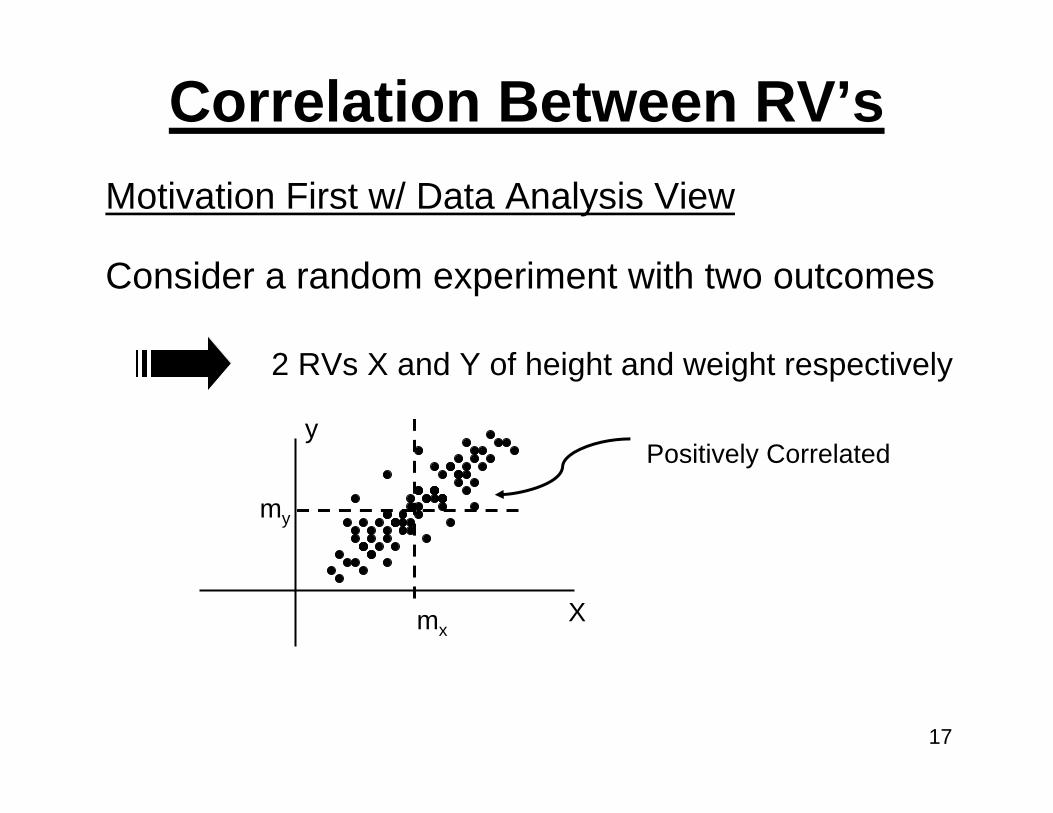
Correlation Between RV’s

Consider a random experiment with two outcomes

2 RVs X and Y of height and weight respectively

y

X

Positively Correlated

mx

my

Motivation First w/ Data Analysis View

18

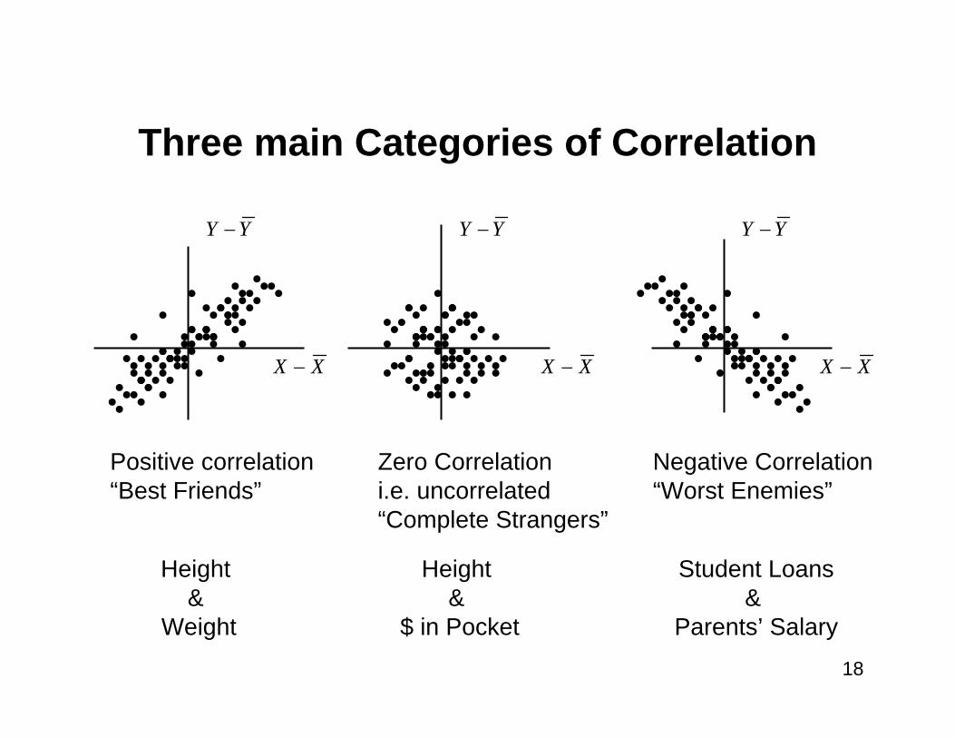
Three main Categories of Correlation

Positive correlation“Best Friends”

Negative Correlation“Worst Enemies”

Zero Correlationi.e. uncorrelated“Complete Strangers”

Height &

Weight

Height &

$ in Pocket

Student Loans&

Parents’ Salary

YY − YY − YY −

XX −XX −XX −

19

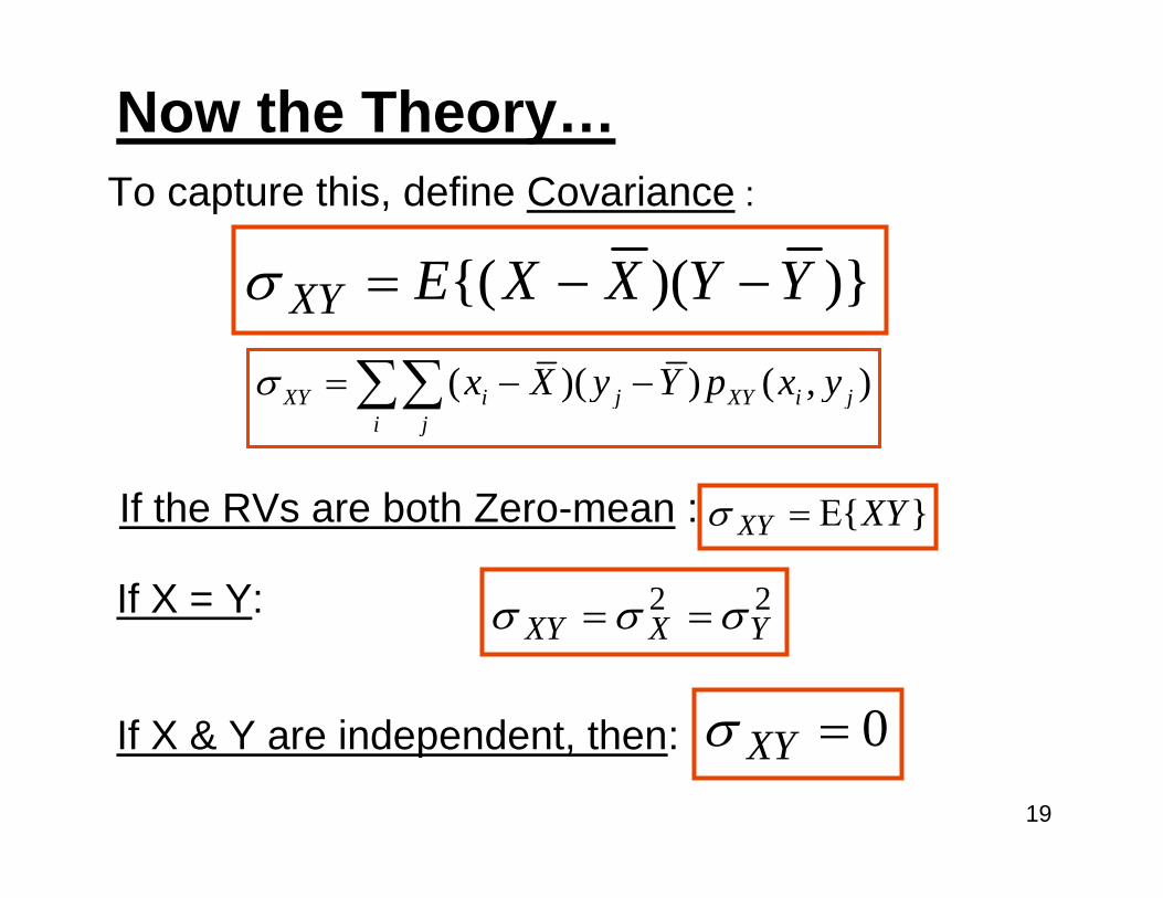
To capture this, define Covariance :

If the RVs are both Zero-mean :

)})({( YYXXEXY −−=σ

}{XYXY Ε=σ

If X = Y: 22YXXY σσσ ==

If X & Y are independent, then: 0=XYσ

Now the Theory…

( )( ) ( , )XY i j XY i ji j

x X y Y p x yσ = − −∑∑

20

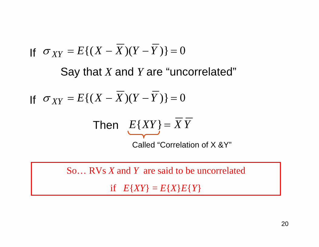
If 0)})({( =−−= YYXXEXYσ

Say that X and Y are “uncorrelated”

If 0)})({( =−−= YYXXEXYσ

Then YXXYE =}{

Called “Correlation of X &Y”

So… RVs X and Y are said to be uncorrelated

if E{XY} = E{X}E{Y}

21

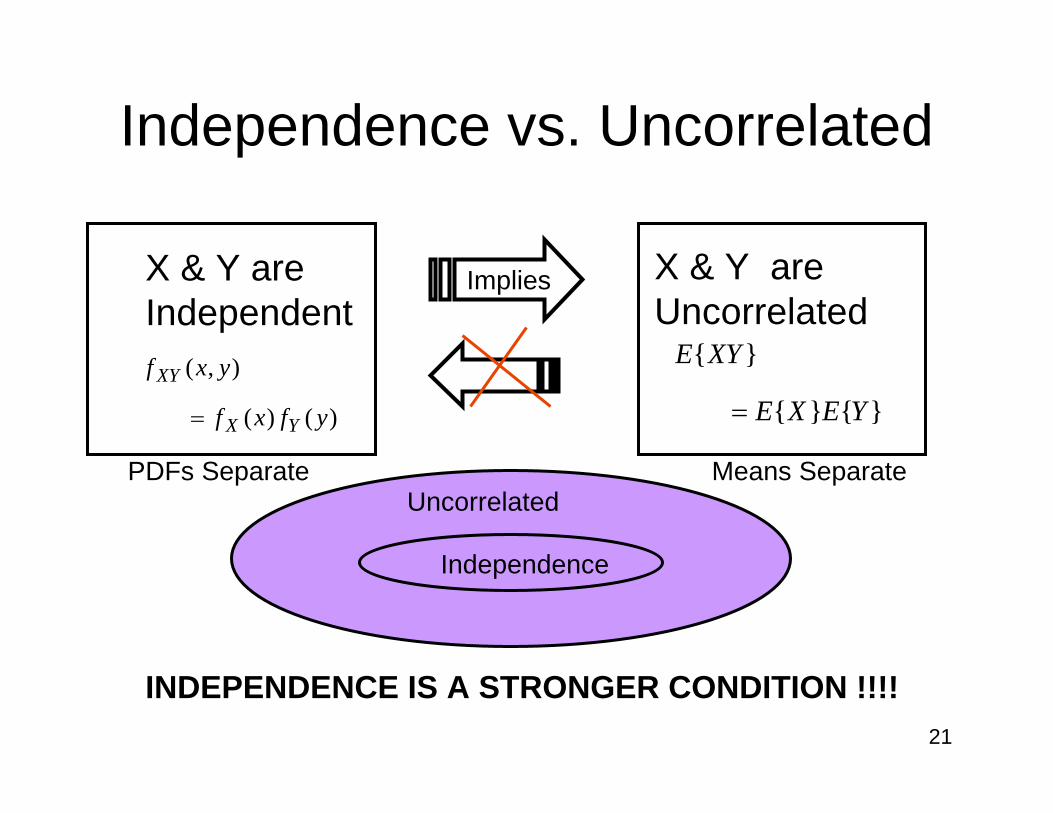
X & Y are Independent

Implies X & Y are Uncorrelated

Uncorrelated

Independence

INDEPENDENCE IS A STRONGER CONDITION !!!!

)()(

),(

yfxf

yxf

YX

XY

= }{}{

}{

YEXE

XYE

=

Independence vs. Uncorrelated

PDFs Separate Means Separate

22

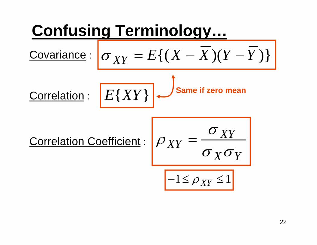
Covariance : )})({( YYXXEXY −−=σConfusing Terminology…

Correlation : }{XYE

Correlation Coefficient :YX

XYXY σσ

σρ =

11 ≤≤− XYρ

Same if zero mean

23

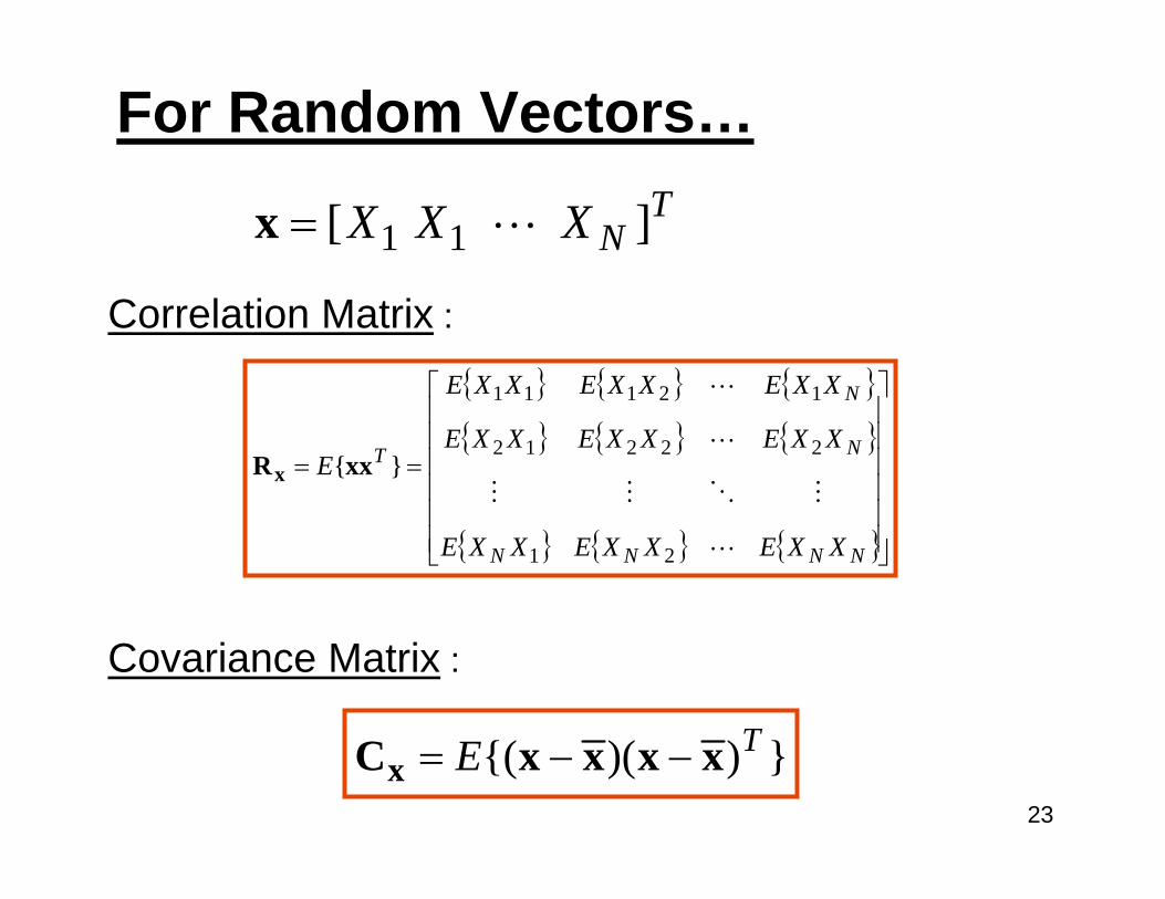
Correlation Matrix :

{ } { } { }{ } { } { }

{ } { } { }⎥⎥⎥⎥⎥⎥

⎦

⎤

⎢⎢⎢⎢⎢⎢

⎣

⎡

==

NNNN

N

N

T

XXEXXEXXE

XXEXXEXXE

XXEXXEXXE

E

21

22212

12111

}{xxRx

For Random Vectors…T

NXXX ][ 11=x

Covariance Matrix :

}))({( TE xxxxCx −−=