Focused fine-tuning of ridge regression

Kristoffer Hellton

Department of Mathematics, University of Oslo

May 9, 2016

K. Hellton (UiO) Focused tuning May 9, 2016 1 / 22

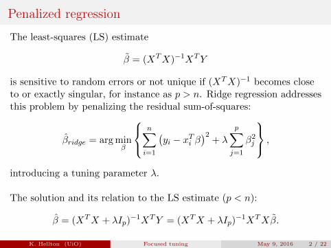
Penalized regression

The least-squares (LS) estimate

β = (XTX)−1XTY

is sensitive to random errors or not unique if (XTX)−1 becomes closeto or exactly singular, for instance as p > n. Ridge regression addressesthis problem by penalizing the residual sum-of-squares:

βridge = arg minβ

n∑i=1

(yi − xTi β

)2+ λ

p∑j=1

β2j

,

introducing a tuning parameter λ.

The solution and its relation to the LS estimate (p < n):

β = (XTX + λIp)−1XTY = (XTX + λIp)

−1XTXβ.

K. Hellton (UiO) Focused tuning May 9, 2016 2 / 22

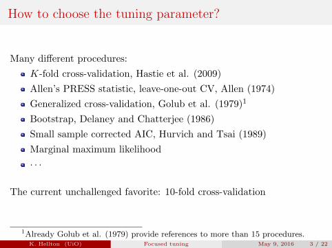
How to choose the tuning parameter?

Many different procedures:

K-fold cross-validation, Hastie et al. (2009)

Allen’s PRESS statistic, leave-one-out CV, Allen (1974)

Generalized cross-validation, Golub et al. (1979)1

Bootstrap, Delaney and Chatterjee (1986)

Small sample corrected AIC, Hurvich and Tsai (1989)

Marginal maximum likelihood

· · ·

The current unchallenged favorite: 10-fold cross-validation

1Already Golub et al. (1979) provide references to more than 15 procedures.K. Hellton (UiO) Focused tuning May 9, 2016 3 / 22

Thought experiment

A medical study has measured covariates and observed outcomes for agroup of patients. A new patient enters the doctors office, and we wishto predict the outcome for his/her specific set of covariates, x0, as bestas possible.

Cross-validation would select λ to be optimal for the overalldistribution of covariates, but not the specific x0.

Instead; frame the specific prediction µ = xT0 β as a focus parameter:

1 find the bias and variance of µ,

2 and minimize the estimated mean squared error (MSE) of µ as afunction of λ to find λ.

K. Hellton (UiO) Focused tuning May 9, 2016 4 / 22

Given the standard fixed designregression model

yi = xTi β + εi, εi ∼ N(0, σ2),

and the focus

µ0 = Ey0 = xT0 β,

the MSE(µ) is a function of λ andthe model parameters: 0 2 4 6 8 10

1.3

01.3

51.4

01.4

5

Tuning parameter

roo

t m

se

MSE(µ;λ, x0, β, σ2) =

{xT0 ((XTX + λIp)

−1XTX − Ip)β}2

+ σ2xT0 (XTX + λIp)−1XTX(XTX + λIp)

−1x0

For each covariate set x0 the MSE curves, as functions of λ, havedifferent minima.

K. Hellton (UiO) Focused tuning May 9, 2016 5 / 22

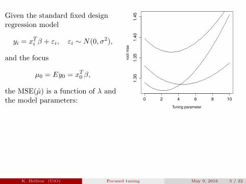
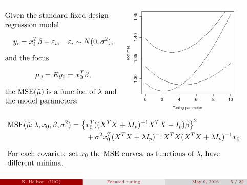
Given the standard fixed designregression model

yi = xTi β + εi, εi ∼ N(0, σ2),

and the focus

µ0 = Ey0 = xT0 β,

the MSE(µ) is a function of λ andthe model parameters: 0 2 4 6 8 10

1.3

01.3

51.4

01.4

5

Tuning parameter

roo

t m

se

MSE(µ;λ, x0, β, σ2) =

{xT0 ((XTX + λIp)

−1XTX − Ip)β}2

+ σ2xT0 (XTX + λIp)−1XTX(XTX + λIp)

−1x0

For each covariate set x0 the MSE curves, as functions of λ, havedifferent minima.

K. Hellton (UiO) Focused tuning May 9, 2016 5 / 22

The minimand of the theoretical MSE defines the oracle tuning

λbest = arg minλ

MSE(µ;λ, x0).

But an estimator of λbest requires pilot estimates of β and σ2.Our proposed estimator uses the LS estimates (for p < n):

λ∗best = arg minλ

MSE(µ;λ, x0),

= arg minλ

Var(µ;λ, x0) + bias2(µ;λ, x0)

= arg minλ

{Var + max{(bias)2 −Var bias, 0}

},

or a simplified version without bias correction, written out as:

λbest = arg minλ

{(xT0 ((XTX + λIp)

−1XTX − Ip)β)2

+σ2xT0 (XTX + λIp)−1XTX(XTX + λIp)

−1x0}

K. Hellton (UiO) Focused tuning May 9, 2016 6 / 22

The minimand of the theoretical MSE defines the oracle tuning

λbest = arg minλ

MSE(µ;λ, x0).

But an estimator of λbest requires pilot estimates of β and σ2.Our proposed estimator uses the LS estimates (for p < n):

λ∗best = arg minλ

MSE(µ;λ, x0),

= arg minλ

Var(µ;λ, x0) + bias2(µ;λ, x0)

= arg minλ

{Var + max{(bias)2 −Var bias, 0}

},

or a simplified version without bias correction, written out as:

λbest = arg minλ

{(xT0 ((XTX + λIp)

−1XTX − Ip)β)2

+σ2xT0 (XTX + λIp)−1XTX(XTX + λIp)

−1x0}

K. Hellton (UiO) Focused tuning May 9, 2016 6 / 22

The minimand of the theoretical MSE defines the oracle tuning

λbest = arg minλ

MSE(µ;λ, x0).

But an estimator of λbest requires pilot estimates of β and σ2.Our proposed estimator uses the LS estimates (for p < n):

λ∗best = arg minλ

MSE(µ;λ, x0),

= arg minλ

Var(µ;λ, x0) + bias2(µ;λ, x0)

= arg minλ

{Var + max{(bias)2 −Var bias, 0}

},

or a simplified version without bias correction, written out as:

λbest = arg minλ

{(xT0 ((XTX + λIp)

−1XTX − Ip)β)2

+σ2xT0 (XTX + λIp)−1XTX(XTX + λIp)

−1x0}

K. Hellton (UiO) Focused tuning May 9, 2016 6 / 22

In one dimension

Suppose p = 1, then

β =M

M + λβ, M =

n∑i=1

x2i ,

and the mean squared error is given

MSE(µ;λ) = x20M2β2

(λ

M + λ

)2

+ x20σ2M

(1

M + λ

)2

,

such that the minimand λbest does not depend on x0!

Our proposed estimator “loses its focus”, more interesting with p ≥ 2.

K. Hellton (UiO) Focused tuning May 9, 2016 7 / 22

Orthogonal case

For general p, assume σ2 to be known and the design matrix to beorthogonal with equal Mj :

XTX = diag(M1, . . . ,Mp) = M Ip.

Then the estimated bias based on the LS pilot estimate is

bias = − λ

M + λxT0 β ∼ Np

(− λ

M + λxT0 β,

σ2λ2xT0 x0M(M + λ)2

),

giving the estimated mean squared error as

MSE(µ;λ) =

(xT0 β −

σ2xT0 x0M

)+

(λ

M + λ

)2

+σ2xT0 x0M

(M

M + λ

)2

,

where (·)+ = max(·, 0).

K. Hellton (UiO) Focused tuning May 9, 2016 8 / 22

Orthogonal case

For general p, assume σ2 to be known and the design matrix to beorthogonal with equal Mj :

XTX = diag(M1, . . . ,Mp) = M Ip.

Then the estimated bias based on the LS pilot estimate is

bias = − λ

M + λxT0 β ∼ Np

(− λ

M + λxT0 β,

σ2λ2xT0 x0M(M + λ)2

),

giving the estimated mean squared error as

MSE(µ;λ) =

(xT0 β −

σ2xT0 x0M

)+

(λ

M + λ

)2

+σ2xT0 x0M

(M

M + λ

)2

,

where (·)+ = max(·, 0).

K. Hellton (UiO) Focused tuning May 9, 2016 8 / 22

Orthogonal case

For general p, assume σ2 to be known and the design matrix to beorthogonal with equal Mj :

XTX = diag(M1, . . . ,Mp) = M Ip.

Then the estimated bias based on the LS pilot estimate is

bias = − λ

M + λxT0 β ∼ Np

(− λ

M + λxT0 β,

σ2λ2xT0 x0M(M + λ)2

),

giving the estimated mean squared error as

MSE(µ;λ) =

(xT0 β −

σ2xT0 x0M

)+

(λ

M + λ

)2

+σ2xT0 x0M

(M

M + λ

)2

,

where (·)+ = max(·, 0).

K. Hellton (UiO) Focused tuning May 9, 2016 8 / 22

Focused tuning estimate

The minimand, our focused tuning estimator, is

λ∗best =σ2MxT0 x0(

M(xT0 β)2 − σ2xT0 x0)+

,

resulting in the focused prediction

y(λ∗best) =

0 if xT0 β ≤ σ‖x0‖/

√M,

M(xT0 β)2 − σ2xT0 x0M(xT0 β)2

xT0 β if xT0 β > σ‖x0‖/√M,

when σ2 known and XTX = diag(M1, . . . ,Mp) = M Ip.

K. Hellton (UiO) Focused tuning May 9, 2016 9 / 22

Simplified focused tuning estimate

In the orthogonal case, the simplified mean squared error without thebias correction is given

MSE(µ;λ) = (xT0 β)2(

λ

M + λ

)2

+ σ2xT0 x0

(M

M + λ

)2

,

with the minimand, the simplified focused tuning

λbest = σ2xT0 x0

(xT0 β)2.

The prediction has a geometric interpretation in terms of α, the anglebetween vectors x0 and β and R2 = ‖x0‖2/‖β‖2:

y(λbest) =M(xT0 β)2

M(xT0 β)2 + σ2xT0 x0xT0 β =

M cos2 α

M cos2 α+ σ2R2xT0 β.

K. Hellton (UiO) Focused tuning May 9, 2016 10 / 22

Simplified focused tuning estimate

In the orthogonal case, the simplified mean squared error without thebias correction is given

MSE(µ;λ) = (xT0 β)2(

λ

M + λ

)2

+ σ2xT0 x0

(M

M + λ

)2

,

with the minimand, the simplified focused tuning

λbest = σ2xT0 x0

(xT0 β)2.

The prediction has a geometric interpretation in terms of α, the anglebetween vectors x0 and β and R2 = ‖x0‖2/‖β‖2:

y(λbest) =M(xT0 β)2

M(xT0 β)2 + σ2xT0 x0xT0 β =

M cos2 α

M cos2 α+ σ2R2xT0 β.

K. Hellton (UiO) Focused tuning May 9, 2016 10 / 22

Prediction risk: p = 1

Risk as function of β with original and simplified focused tuning:

−3 −2 −1 0 1 2 3

0.4

0.6

0.8

1.0

1.2

1.4

Risk for original FIC (black) and adjusted FIC (red)

Regression parameter Beta

Ris

k

Both do better then least-squares (scaled to 1) for small β. Theoriginal is better then the simplified for β close to zero, but worse formedium β. NB: it does not depend on x0.

K. Hellton (UiO) Focused tuning May 9, 2016 11 / 22

Prediction risk: p = 2

For p ≥ 2, the prediction risk risk(xT0 β(λbest)) will vary with x0.

For the simplified tuning, the risk surface as function of β (for fixed x0)shows a trench orthogonal to x0:

−10 −5 0 5 10−10

−5

0

510

Ris

k

0.2

0.4

0.6

0.8

1.0

1.2

Risk surface

−10 −5 0 5 10−10

−5

0

5

10

Ris

k

0.2

0.4

0.6

0.8

1.0

1.2

Risk surface

K. Hellton (UiO) Focused tuning May 9, 2016 12 / 22

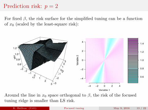
Prediction risk: p = 2

For fixed β, the risk surface for the simplified tuning can be a functionof x0 (scaled by the least-square risk):

x1

−3−2

−1

0

1

2

3

x2

−3

−2

−1

0

1

2

3

risk

0.6

0.8

1.0

1.2

Risk surface as function of x0

0.6

0.8

1.0

1.2

1.4

−4 −2 0 2 4

−4

−2

0

2

4

Risk surface for FIC

Variable 1

Vari

able

2

Around the line in x0 space orthogonal to β, the risk of the focusedtuning ridge is smaller than LS risk.

K. Hellton (UiO) Focused tuning May 9, 2016 13 / 22

Cross-validation

K-fold cross-validation has emerged as a standard for selecting tuningparameters. We will study n-fold or leave-one-out cross-validation

λCV = arg minλ

n∑i=1

(yi − xTi β−i,λ

)2where the ith observation is removed from the model fitting whenpredicting yi. For ridge regression, the leave-one-out cross-validationcriterion simplifies to weighted sum of squared residuals:

CV (λ) =

n∑i=1

(yi − xTi βλ1−Hii,λ

)2

,

where H = X(XTX + λ)−1XT , the weights, quantify the distance ofthe covariates from the centroid (Golub et al. 1979).

K. Hellton (UiO) Focused tuning May 9, 2016 14 / 22

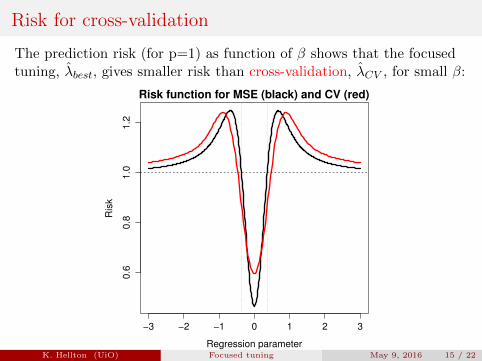
Risk for cross-validation

The prediction risk (for p=1) as function of β shows that the focusedtuning, λbest, gives smaller risk than cross-validation, λCV , for small β:

−3 −2 −1 0 1 2 3

0.6

0.8

1.0

1.2

Risk function for MSE (black) and CV (red)

Regression parameter

Ris

k

K. Hellton (UiO) Focused tuning May 9, 2016 15 / 22

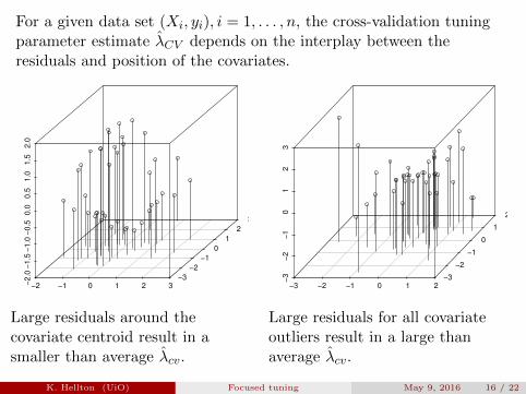
For a given data set (Xi, yi), i = 1, . . . , n, the cross-validation tuningparameter estimate λCV depends on the interplay between theresiduals and position of the covariates.

−2 −1 0 1 2 3−2.0

−1.5

−1.0

−0.5

0.0

0.5

1.0

1.5

2.0

−3

−2

−1

0

1

2

3

Large residuals around thecovariate centroid result in asmaller than average λcv.

−3 −2 −1 0 1 2−

3−

2−

1 0

1 2

3

−3

−2

−1

0

1

2

Large residuals for all covariateoutliers result in a large thanaverage λcv.

K. Hellton (UiO) Focused tuning May 9, 2016 16 / 22

To compare prediction error as function of x0: fix X, simulate fourdifferent {yi}, i = 1, . . . , 40 and color the difference as focused tuningbeing better and cross-validation being better. Thick line: xT0 β = 0.

−0.05

0.00

0.05

−0.3 −0.2 −0.1 0.0 0.1 0.2 0.3

−0.3

−0.2

−0.1

0.0

0.1

0.2

0.3

Difference minimal MSE and CV predition

Variable 1

Va

ria

ble

2

−0.10

−0.05

0.00

0.05

0.10

−0.3 −0.2 −0.1 0.0 0.1 0.2 0.3

−0.3

−0.2

−0.1

0.0

0.1

0.2

0.3

Difference minimal MSE and CV predition

Variable 1

Va

ria

ble

2

−0.2

−0.1

0.0

0.1

0.2

−0.3 −0.2 −0.1 0.0 0.1 0.2 0.3

−0.3

−0.2

−0.1

0.0

0.1

0.2

0.3

Difference minimal MSE and CV predition

Variable 1

Va

ria

ble

2

−0.3

−0.2

−0.1

0.0

0.1

0.2

0.3

−0.3 −0.2 −0.1 0.0 0.1 0.2 0.3

−0.3

−0.2

−0.1

0.0

0.1

0.2

0.3

Difference minimal MSE and CV predition

Variable 1

Va

ria

ble

2

K. Hellton (UiO) Focused tuning May 9, 2016 17 / 22

To compare prediction error as function of x0: fix X, simulate fourdifferent {yi}, i = 1, . . . , 40 and color the difference as focused tuningbeing better and cross-validation being better. Thick line: xT0 β = 0.

−0.05

0.00

0.05

−0.3 −0.2 −0.1 0.0 0.1 0.2 0.3

−0.3

−0.2

−0.1

0.0

0.1

0.2

0.3

Difference minimal MSE and CV predition

Variable 1

Va

ria

ble

2

−0.10

−0.05

0.00

0.05

0.10

−0.3 −0.2 −0.1 0.0 0.1 0.2 0.3

−0.3

−0.2

−0.1

0.0

0.1

0.2

0.3

Difference minimal MSE and CV predition

Variable 1

Va

ria

ble

2

−0.2

−0.1

0.0

0.1

0.2

−0.3 −0.2 −0.1 0.0 0.1 0.2 0.3

−0.3

−0.2

−0.1

0.0

0.1

0.2

0.3

Difference minimal MSE and CV predition

Variable 1

Va

ria

ble

2

−0.3

−0.2

−0.1

0.0

0.1

0.2

0.3

−0.3 −0.2 −0.1 0.0 0.1 0.2 0.3

−0.3

−0.2

−0.1

0.0

0.1

0.2

0.3

Difference minimal MSE and CV predition

Variable 1

Va

ria

ble

2

K. Hellton (UiO) Focused tuning May 9, 2016 17 / 22

To compare prediction error as function of x0: fix X, simulate fourdifferent {yi}, i = 1, . . . , 40 and color the difference as focused tuningbeing better and cross-validation being better. Thick line: xT0 β = 0.

−0.05

0.00

0.05

−0.3 −0.2 −0.1 0.0 0.1 0.2 0.3

−0.3

−0.2

−0.1

0.0

0.1

0.2

0.3

Difference minimal MSE and CV predition

Variable 1

Va

ria

ble

2

−0.10

−0.05

0.00

0.05

0.10

−0.3 −0.2 −0.1 0.0 0.1 0.2 0.3

−0.3

−0.2

−0.1

0.0

0.1

0.2

0.3

Difference minimal MSE and CV predition

Variable 1

Va

ria

ble

2

−0.2

−0.1

0.0

0.1

0.2

−0.3 −0.2 −0.1 0.0 0.1 0.2 0.3

−0.3

−0.2

−0.1

0.0

0.1

0.2

0.3

Difference minimal MSE and CV predition

Variable 1

Va

ria

ble

2

−0.3

−0.2

−0.1

0.0

0.1

0.2

0.3

−0.3 −0.2 −0.1 0.0 0.1 0.2 0.3

−0.3

−0.2

−0.1

0.0

0.1

0.2

0.3

Difference minimal MSE and CV predition

Variable 1

Va

ria

ble

2

K. Hellton (UiO) Focused tuning May 9, 2016 17 / 22

To compare prediction error as function of x0: fix X, simulate fourdifferent {yi}, i = 1, . . . , 40 and color the difference as focused tuningbeing better and cross-validation being better. Thick line: xT0 β = 0.

−0.05

0.00

0.05

−0.3 −0.2 −0.1 0.0 0.1 0.2 0.3

−0.3

−0.2

−0.1

0.0

0.1

0.2

0.3

Difference minimal MSE and CV predition

Variable 1

Va

ria

ble

2

−0.10

−0.05

0.00

0.05

0.10

−0.3 −0.2 −0.1 0.0 0.1 0.2 0.3

−0.3

−0.2

−0.1

0.0

0.1

0.2

0.3

Difference minimal MSE and CV predition

Variable 1

Va

ria

ble

2

−0.2

−0.1

0.0

0.1

0.2

−0.3 −0.2 −0.1 0.0 0.1 0.2 0.3

−0.3

−0.2

−0.1

0.0

0.1

0.2

0.3

Difference minimal MSE and CV predition

Variable 1

Va

ria

ble

2

−0.3

−0.2

−0.1

0.0

0.1

0.2

0.3

−0.3 −0.2 −0.1 0.0 0.1 0.2 0.3

−0.3

−0.2

−0.1

0.0

0.1

0.2

0.3

Difference minimal MSE and CV predition

Variable 1

Va

ria

ble

2

K. Hellton (UiO) Focused tuning May 9, 2016 17 / 22

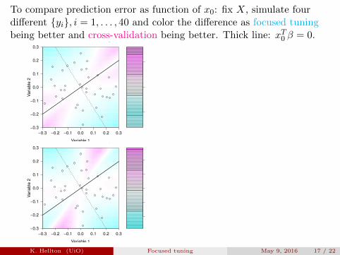
To compare prediction error as function of x0: fix X, simulate fourdifferent {yi}, i = 1, . . . , 40 and color the difference as focused tuningbeing better and cross-validation being better. Thick line: xT0 β = 0.

−0.05

0.00

0.05

−0.3 −0.2 −0.1 0.0 0.1 0.2 0.3

−0.3

−0.2

−0.1

0.0

0.1

0.2

0.3

Difference minimal MSE and CV predition

Variable 1

Va

ria

ble

2

−0.10

−0.05

0.00

0.05

0.10

−0.3 −0.2 −0.1 0.0 0.1 0.2 0.3

−0.3

−0.2

−0.1

0.0

0.1

0.2

0.3

Difference minimal MSE and CV predition

Variable 1

Va

ria

ble

2

−0.2

−0.1

0.0

0.1

0.2

−0.3 −0.2 −0.1 0.0 0.1 0.2 0.3

−0.3

−0.2

−0.1

0.0

0.1

0.2

0.3

Difference minimal MSE and CV predition

Variable 1

Va

ria

ble

2

−0.3

−0.2

−0.1

0.0

0.1

0.2

0.3

−0.3 −0.2 −0.1 0.0 0.1 0.2 0.3

−0.3

−0.2

−0.1

0.0

0.1

0.2

0.3

Difference minimal MSE and CV predition

Variable 1

Va

ria

ble

2

K. Hellton (UiO) Focused tuning May 9, 2016 17 / 22

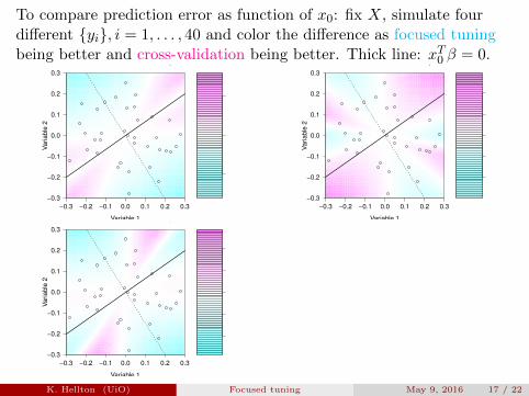
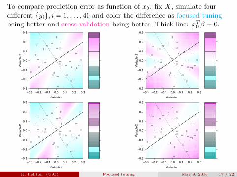
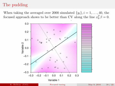
The pudding

When taking the averaged over 2000 simulated {yi}, i = 1, . . . , 40, thefocused approach shows to be better than CV along the line xT0 β = 0.

−0.04

−0.02

0.00

0.02

0.04

−0.3 −0.2 −0.1 0.0 0.1 0.2 0.3

−0.3

−0.2

−0.1

0.0

0.1

0.2

0.3

Difference minimal MSE and CV predition

Variable 1

Vari

able

2

K. Hellton (UiO) Focused tuning May 9, 2016 18 / 22

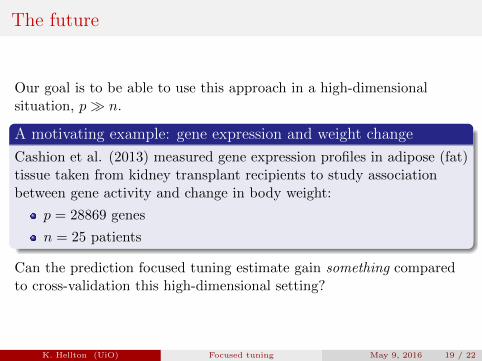
The future

Our goal is to be able to use this approach in a high-dimensionalsituation, p� n.

A motivating example: gene expression and weight change

Cashion et al. (2013) measured gene expression profiles in adipose (fat)tissue taken from kidney transplant recipients to study associationbetween gene activity and change in body weight:

p = 28869 genes

n = 25 patients

Can the prediction focused tuning estimate gain something comparedto cross-validation this high-dimensional setting?

K. Hellton (UiO) Focused tuning May 9, 2016 19 / 22

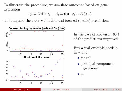
To illustrate the procedure, we simulate outcomes based on geneexpression

yi = Xβ + εi, βj = 0.01, εi ∼ N(0, 1),

and compare the cross-validation and focused (oracle) prediction:

5 10 15 20 25

02

00

05

00

0

Focused tuning parameter (red) and CV (blue)

5 10 15 20 25

01

23

45

6

Root prediction error

In the case of known β: 60%of the predictions improved.

But a real example needs anew pilot:

ridge?

principal componentregression?

...

K. Hellton (UiO) Focused tuning May 9, 2016 20 / 22

Concluding remarks

As shown, the focused tuning estimator gives lower prediction errorcompared to cross-validation for certain x0.

Future work:

controlling overfitting.

find the best pilot estimate in high-dimension. Two-step ridgeregression with cross-validation? PCR?

exploit the low-dimensionality of the projection xT0 β as p grows?

explore further foci; βTβ, individual βi, P [y0 > ythres] = α

K. Hellton (UiO) Focused tuning May 9, 2016 21 / 22

Thank you!

K. Hellton (UiO) Focused tuning May 9, 2016 22 / 22