Fock and Coherent

THE INTERACTION OF RADIATION AND MATTER: QUANTUM THEORY PAGE 19

R. Victor Jones, May 2, 200019

III. REPRESENTATIONS OF PHOTON STATES

1. Fock or “Number” States : .11

As we have seen, the Fock or number states

n r k { } ≡ ∏

s σn r

k s σ [ III-1 ]

are complete set eigenstates of an important group of commuting observables -- viz.H rad , N and

r M .

Reprise of Characteristics and Properties of Fock States:

a. The expectation value of the number operator and the fractional

uncertainty associated with a single Fock state:

n N n = n [ III-2a ]

∆n = "uncertainty" [ ] = n N 2 n − n N n2{ } = 0 [ III-2b ]

b. Expectation value of the fields associated with a single mode:

For one mode Equations [ II-24a ] and [ II-24b ] reduce to

r E

r r , t( ) = i ˆ e E a exp i

r k ⋅

r r − i ω t[ ] − a † exp −i

r k ⋅

r r − i ω t[ ]

[ III-3a ]

r H

r r , t( ) = i

ε0

µ 0

E ˆ k × ˆ e [ ] a t( ) exp ir k ⋅

r r − i ω t[ ] − a † t( ) exp − i

r k ⋅

r r − i ω t[ ]

[ III-3b ]

11 In what follows, for simplicity we drop the r k subscripts on the operators and state vectors with the obvious

meaning that n r k { } ⇒ n , a r

k ⇒ a , etc...



where E=hω

2ε0 V

nr E n = 0

nr H n = 0 [ III-4a ]

∆E = nr E ⋅

r E n − n

r E n

2{ } = hωε0 V

n + 12( )

12 = 2 E n + 1

2( )1

2

∆H = nr H ⋅

r H n − n

r H n

2{ } =hω

µ 0 Vn + 1

2( )1

2 =ε0

µ 0

2 E n + 12( )

12

∆E ∆H = chωV

n + 12( ) =

ε0

µ 0

2E2 n + 12( )

[ III-4b ]

c. Phase of field associated with single mode:

To obtain something analogous to the classical theory we would like to separate the

creation and destruction operators (and, thus, the electric and magnetic field

operators) into a product of amplitude and phase operators. Following Susskind

and Glogower,12 we define a phase operator , Φ such that

a ≡ N + 1( )12

exp i Φ( )

a† ≡ exp −i Φ( ) N +1( )1

2 [ III-5 ]

Defined in this way, the basic properties of the phase operator may be evaluated

from known properties of the creation, destruction and number operators.

Inverting, we obtain

12 Susskind, L. and Glogower, J., Physics, 1 , 49 (1964)



exp i Φ( ) ≡ N +1( )− 12 a

exp −i Φ( ) ≡ a† N +1( )− 12 [ III-6 ]

and since a a† =N + 1, it follows that

exp i Φ( ) exp −i Φ( ) = 1 [ III-7 ]

but only in this order! Operating on number states with the phase operators,

we obtain from Equation [ I-26 ]

exp i Φ( ) n = N +1( )−12 a n = N +1( )−1

2 n( ) 12 n −1 = n −1

exp − i Φ( ) n = a † N +1( )−12 n = a † n +1( )−1

2 n = n +1[ III-8 ]

Consequently, the only nonvanishing matrix elements of the phase operator

are

n −1 exp i Φ( ) n = 1

n + 1 exp −i Φ( ) n = 1[ III-9 ]

The phase operators defined by Equation [ III-36 ] do have the felicitous or

classically analogous property of revealing magnitude independent

information, but unfortunately they are nonHermitian operators -- i.e.

n −1 exp i Φ( ) n ≠ n exp i Φ( ) n − 1∗

-- and, hence, cannot represent observables. However, they may be paired

into operators that are observables -- viz.



cosΦ = 1

2exp i Φ( ) + exp −i Φ( ){ }

sinΦ = 1

2 iexp i Φ( ) − exp −i Φ( ){ }

[ III-10 ]

which have the following nonvanishing matrix elements:

n −1 cosΦ n = n cosΦ n −1 = 1

2

n −1 sin Φ n = − n sin Φ n −1 = 1

2 i

[ III-11 ]

These nearly commuting operators13 may be adopted as the quantum mechanical

operators which represent (as we will demonstrate anon) the observable phase

properties of the electromagnetic field.

For the Fock state:

n cos Φ n = n sinΦ n = 0 [ III-12a ]

∆ cos Φ = ∆sin Φ= n cos2 Φ n − n cosΦ n2{ } = 1

2 [ III-12b ]

∆ cosΦ ∆ sin Φ = 12

[ III-12c ]

c. The coordinate or Schrödinger representation of state:

Recall from Equations [ I-10a ] and [I-31] that

13 Also, it may be easily established that the matrix elements of their commutator are given by

n cos Φ,sinΦ[ ] ′ n =i

2δn ′ n δn0



q n =1

n !

m

2 hω

n

ω q−hm

d

dq

n

q 0

=1

2n n!

ωπ h

H n

m ωh

q

exp −

m ω2 h

q2

[ III-13 ]

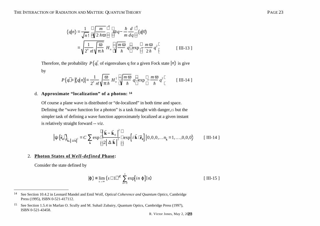
Therefore, the probability P q( ) of eigenvalues q for a given Fock state n is give

by

P q( ) = q n =1

2n n!

ωπ h

H n2 m ω

hq

exp −

m ωh

q2

[ III-14 ]

d. Approximate “localization” of a photon: 14

Of course a plane wave is distributed or “de-localized” in both time and space.

Defining the “wave function for a photon” is a task fraught with danger,15 but the

simpler task of defining a wave function approximately localized at a given instant

is relatively straight forward -- viz.

ψr r 0( ) r

k 0 ∆r k

2 = C exp

r k −

r k 0

2

2 ∆r k

2

exp ir k ⋅

r r 0[ ] 0,0,0,Knr

k =1,K ,0,0,0r k

∑ [ III-14 ]

2. Photon States of Well-defined Phase :

Consider the state defined by

ϕ ≡ lims →∞

s + 1( )− 12 exp in ϕ[ ] n

n= 0

s

∑ [ III-15 ]

14 See Section 10.4.2 in Leonard Mandel and Emil Wolf, Optical Coherence and Quantum Optics, Cambridge

Press (1995), ISBN 0-521-417112.

15 See Section 1.5.4 in Marlan O. Scully and M. Suhail Zubairy, Quantum Optics, Cambridge Press (1997),ISBN 0-521-43458.



Clearly, ϕ ϕ =1 given the orthonormal properties of the number states. Essential

question: Is this state an eigenstate of the phase operators? To answer the question we

need to consider the following potential eigenvalue equation:

cosΦ ϕ =1

2lims→∞

s+1( )−12 exp i n ϕ[ ] exp i Φ[ ] n + exp in ϕ[ ] exp − i Φ[ ] n

n=0

s

∑n=0

s

∑

[ III-16a ]

Using Equations [ III-10 ] and [ III-10 ], we obtain

cosΦ ϕ =1

2lims→∞

s +1( )− 12 exp in ϕ[ ] n − 1 + exp i n ϕ[ ] n +1

n= 0

s

∑n =1

s

∑

=1

2lims→∞

s +1( )− 12 exp iϕ( ) exp i ν ϕ[ ] ν + exp −i ϕ[ ] exp i ν ϕ[ ] ν

ν = 1

s +1

∑ν = 0

s− 1

∑

= cosϕ ϕ

+ 12

lims→∞

s +1( )− 12 exp i s ϕ[ ] s +1 − exp i s + 1( ) ϕ[ ] s − exp −i ϕ[ ] 0{ }

[ III-16b ]

so that the state ϕ fails to be a strict eigenket of cosΦ by terms that diminish faster

than s + 1( )− 12 as s →∞ . Similarly, we can see that diagonal matrix elements of cosΦ

and sinΦ are given by

ϕ cos Φ ϕ = cosϕ 1− lims →∞

s + 1( )−1{ } ⇒ cosϕ [ III-17a ]

ϕ sin Φ ϕ = sinϕ 1− lims→∞

s + 1( )−1{ } ⇒ sinϕ [ III-17b ]



Reprise of Characteristics and Properties of Phase States:

a. The expectation value of the number operator and the fractional

uncertainty associated with a state of well-defined phase:

ϕ N ϕ = lim

s →∞s + 1( )−1

nn = 0

s

∑ = lims→∞

s +1( )− 1 s s +1( )2

= lim

s→∞

s

2[ III-18a ]

fractional

uncertainty

=

ϕ N 2 ϕ − ϕ N ϕ 2{ }ϕ N ϕ

=

lims→∞

s+1( )−1n2

n=0

s

∑ − lims→∞

s+1( )−1n

n=0

s

∑

2

lims→∞

s+1( )−1n

n=0

s

∑

=lims→∞

1

62s2 + s( ) −

1

4s2

lims→∞

s2

= 1

3

[ III-18b ]

b. Expectation value of the fields associated with a single mode:

From Equation [ III-3a ]

ϕr E ϕ =− 2

h ω2 ε0 V

ˆ e sinr k ⋅

r r − ω t + ϕ( ) lim

s →∞s + 1( )−1 n + 1( )1

2

n= 0

s

∑⇒ diverges as s for large s !

[ III-19 ]



c. Phase of field associated with single mode:

ϕ cosΦ ϕ = cosϕ

ϕ sinΦ ϕ = sinϕ[ III-20a ]

∆ cos Φ = ∆sin Φ= ϕ cos2 Φ ϕ − ϕ cosΦ ϕ 2{ } = 0 [ III-20b ]

d. Probability of photon number:

Finally, we may easily deduce the probability of finding n photons (i.e. the photon

statistics) in a particular state of well defined phase -- viz.

Pn = n ϕ2

≡ lims →∞

s + 1( )−1[ III-50 ]

We see that there is a equal, but small probability of any number: this agrees with the

intuition that the magnitude of the field is completely undetermined if the phase is

precisely known!

3. Coherent Photon States: 16

It would, indeed, be useful to have eigenstates of the destruction operator (electric

or magnetic field) -- viz.

a r k α r

k = α r k α r

k [ III-51 ]

Reprise of Characteristics and Properties of Coherent States:

a. The Fock state representation of the coherent state:

16 The coherent state is a Harvard invention! See R. J. Glauber, Phys. Rev. 131 , 2766 (1963).



Since. a † n = n +1 n +1 and a a † = N +1 , then n a = n +1 n +1 and we

are able to write a representative of the sought state in the number state basis -- viz.

n a α = n +1 n +1 α = α n α [ III-52a ]

or n α =αn

n −1 α =αn

n!0 α [ III-52b ]

Using the expansion of the identity operator, the eigenket becomes

α = n n αn

∑ = 0 ααn

n!n

n

∑ . [ III-53 ]

To normalize the eigenket write

α α = α 0 0 αα∗n

αn

n!n

∑ = α 0 0 α exp α2[ ] = 1 [ III-54 ]

so that α 0 = 0 α = exp −1

2α

2

. Finally, we see that

α = exp −1

2α

2

αn

n!n

n

∑ [ III-55 ]

is a normalize representation of the eigenkets of the destruction operator.



b. The expectation value of the number operator and the fractional

uncertainty associated with a coherent state:

α N α = α 2[ III-56a ]

fractional

uncertainty

=

α N 2 α − α N α 2{ }α N α

= 1

α 2exp −α 2( ) α 2n

n!n2∑ − α 4

=1

α 2 exp −α 2( ) α2n

n!n n −1( ) + n[ ]∑ − α 4

= α −1

[ III-56b ]

Thus, we see that the fractional uncertainty diminishes with mean photon number!

c. Expectation value of the electric field associated with a single mode:

From Equation [ III-3a ]

α

r E α = −2

h ω2 ε0 V

ˆ e α sinr k ⋅

r r −ω t +ϑ( ) [ III-57a ]

where α= α exp i ϑ( ) .

∆E = αr E ⋅

r E α − α

r E α

2{ } =h ω

2ε0 V17 [ III-57b ]

17 Similarly

∆H=

1

c µ0

h ω2 ε0 V

for the coherent state, so that ∆E ∆H = c h ω 2 V .



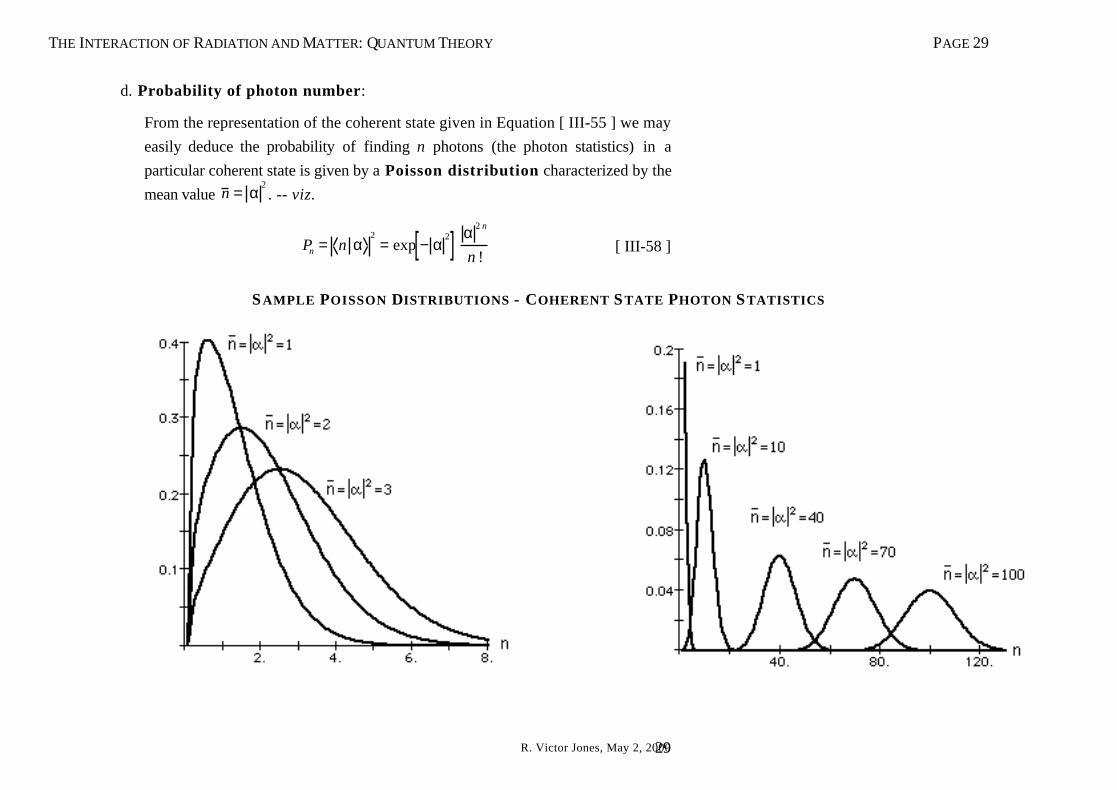
d. Probability of photon number:

From the representation of the coherent state given in Equation [ III-55 ] we may

easily deduce the probability of finding n photons (the photon statistics) in a

particular coherent state is given by a Poisson distribution characterized by the

mean value n = α2. -- viz.

Pn = n α2

= exp − α2[ ] α 2 n

n ![ III-58 ]

SAMPLE POISSON DISTRIBUTIONS - COHERENT STATE PHOTON STATISTICS



e. Phase of field associated with single mode:

α cos Φ α = 1

2exp − 1

2α 2

′ n

α∗ ′ n

′ n !N +1( )− 1

2 a +a† N + 1( )−12[ ] αn

n !n

n∑

′ n ∑

=1

2exp −

1

2α 2

α∗n +1α n + α∗n

αn +1

n + 1( )! n!{ }

n

∑

= α cosϑ exp − 1

2α 2

α 2n

n! n +1( )

n∑

[ III-59a]

Unfortunately, it is not possible to evaluate this summation analytically. However,

Carruthers18 has given an asymptotic expansion which is valid for a large mean

number of photons -- viz.

α cos Φ α = cosϑ 1 −

1

8 α 2 +K

α 2 >> 1 [ III-59b]

f. Coherent states as a basis:

As we will see presently, the coherent states are very useful in describing the

quantized electromagnetic field, but, alas, there is a complication -- the coherent

states are not truly orthogonal! From Equation [ III-6 ] we see that

β α = exp − 12

α 2 − 12

β 2

β∗nαn

n !n

∑

= exp − 12

α 2 − 12

β 2 +αβ∗

[ III-60 ]

so that

18 Carruthers, P. and Nieto, M. M., Phys. Rev. Lett. 14 , 387 (1965)



αβ β α = exp −α2− β

2+αβ∗ +α∗ β( )

= exp − α−β( ) α∗ −β∗( )( ) = exp − α−β2( ) [ III-61 ]

That is, the eigenkets are approximately orthogonal only when α−β is

large!

g. The “displacement operator:”

There are a growing and significant set of applications where it is useful to express

the coherent states directly in terms of the vacuum state 0 . If we use the number

state generating rule

n =a †

n

n !0

-- i.e. Equation [ I-27 ] -- the coherent state may be written in the form

α = exp −1

2α

2

α a †

n

n !0

n

∑ = exp α a † −1

2α

2

0 [ III-62 ]

If we make us of the Baker-Hausdorff theorem,19 we may easily show that

19 The Baker-Hausdorff theorem or identity may be stated as

exp A +B{ } = exp A{ } exp B{ } exp − 12 A ,B[ ]{ }

when A , A ,B[ ][ ] = B , A ,B[ ][ ] = 0 . For a proof, see, for example, Charles P. Slichter’s Principles of

Magnetic Resonance, Appendix A or William Louisell’s Radiation and Noise in Quantum Electronics.



α = A † α( ) 0 = exp α a † − α∗ a

0 [ III-63 ]

so that A † α( ) may be interpreted as a creation operator which generates a

coherent state from the vacuum. (Its adjoint operator A α( ) = A † −α( ) is a

destruction operator which destroys a state). In some treatments A † α( ) is

described as the “displacement operator” (written D α( ) )20 and the coherent states

are called the “displaced states of the vacuum.” 21

To explore this point of view (and to give some meaning to the phase of thecoherent state eigenvalue), we may express α in a two-dimensional,

dimensionless “phase space” representation. To that end, following Equation

[ I-16 ], we write the dimensionless coordinate as

θ =2 mω

h

12

q = a † exp i γ[ ] +a exp − i γ[ ] [ III-64a ]

and the dimensionless momentum as

π = 2

m hω

12

p = a † exp i γ + π 2( )[ ] +a exp − i γ + π 2( )[ ] [ III-64b ]

so that θ , π[ ] = 2 i a ,a †

= 2 i [ III-64c ]

20 We can (or rather you will) show that D † α( ) a D α( ) = a + α and D † α( ) a † D α( ) = a † + α∗

21 See Elements of Quantum Optics, Pierre Meystre and Murray Sargent III, Spinger-Verlag (1991), ISBN 0-387-54190-X.



and since these variables are canonical 22

∆ θ( )2∆ π( )2

≥ 1 [ III-64d ]

Since

a † = 1

2θ− i π( ) exp − i γ[ ]

a =12

θ + i π( ) exp i γ[ ][ III-65 ]

the mode field (see Equation [II-24a]) b

r E

r r , t( ) = i ˆ e E a exp i

r k ⋅

r r − i ω t[ ] − a † exp − i

r k ⋅

r r + i ω t[ ]

[ III-66a ]

becomes

r E

r r , t( ) = − ˆ e E π cos

r k ⋅

r r −ω t +γ( ) +θ sin

r k ⋅

r r −ω t +γ( ){ } [ III-66b ]

Since p has a coordinate space representation −i h d dq = − i h ω 2( ) 12 d d θ

and q has a momentum representation i h d d p = i h 2 ω( ) 12 d d π , 23

αa † − α∗ a = αr a † − a

+ i αi a † +a

=− αr d d θ +α i d d π[ ] [ III-67a ]

22 Of course, in general ∆ A( )2∆ B( )2

≥1

2A ,B[ ]

2

where ∆ A( )2= A 2 − A

2

23 If this unfamiliar, see Equations [ I-20 ] and [ I-22 ] in the lecture notes entitled The Interaction of Radiationand Matter: Semiclassical Theory.



and

A † α( ) = exp αa † − α∗ a

= exp − αr d d θ +α i d d π( )[ ] [ III-67b ]

Thus, A† α( ) defines or generates a two-dimensional Taylor expansion when it

acts on a function of θ and π . In particular, if we take the “phase space”representation of the ground or vacuum state θπ as the product of two Gaussians

(see Equations [ I-10a ] and [ I-29 ]), then A † α( ) θπ represents a shift or

displacement of this “phase space” representation -- i.e.

θπ α = θπ A † α( ) 0 = uG θ− αr( ) uG π − αi( ) [ III-68 ]

In light of Equation [ II-23b ], α t( ) = α exp − i ω t( ) we can write

θπ α t( ) = uG θ− α cos ω t +φ( )( ) uG π − α cos ω t +φ( )( ) [ III-69 ]

where α= α exp i φ( ) .

h. The diagonal coherent-state representation of the density operator

(Glauber-Sudarshan P-representation):

It may be easily established that

1 =1

πβ β d2 β∫∫ = β β d Re β( ) d Im β( )∫∫ [ III-70 ]

so that it seems quite reseasonable to look for a representation of the density matrix

is the form

ρ = P β( ) β β d2 β∫∫ [ III-71 ]

For a pure coherent state, P is clearly a two-dimensional delta function



Example 1 -- Coherent state

P β( ) = δ 2( ) β− α( ) =δ 1( ) Re β( ) − Re α( )( ) δ 1( ) Im β( ) − Im α( )( ) [ III-72 ]

In general, using Equation [ III-60 ] -- i.e.

β α = exp −1

2α

2−

1

2β

2+αβ∗

[ III-60 ]

we may find a simple procedure for finding the P-representation by writing

−α ρ α = P β( ) −α β β α d2 β∫∫= exp − α

2( ) P β( ) exp −β2( )

exp αβ∗ −β α∗[ ] d2 β∫∫[III-73 ]

Thus, −α ρ α exp − α2( ) is the two-dimensional Fourier transform 0f the

function P β( ) exp −β2( ) and we may write

P β( ) =1

π 2 exp β2( ) −α ρ α exp α

2( )∫∫ exp −αβ∗ +β α∗[ ] d2 α [ III-74 ]

As a second example, consider a thermal radiation field described by a canonical

ensemble

ρ =exp − H kB T( )

Tr exp − H kB T( )[ ] [III-75 ]

where H = hω a † a +1

2

. Thus,

ρ = 1− exph ωkB T

exp −n hωkB T

n

∑ n n [III-76 ]



and n = Tr ρ a † a

= exp

hωkB T

−1

−1

n

∑ [III-77 ]

so that ρ =n

n

1+ n( )n+1n

∑ n n [III-78 ]

Thus, we can write n ρ n =n

n

1+ n( )n+1 [III-79 ]

and

−α ρ α =n

n

1+ n( )n+1n

∑ −α n n α

=exp −α 2( )

1+ n

−α 2( )n

n!n

∑ n

1+ n( )

n

=exp −α 2( )

1+ nexp −α 2

1+ 1n

[III-80 ]

Finally, we see that

Example 2 -- Thermal radiation - a chaotic state

P α( ) =exp α 2( )π 2 1+ n( ) exp −β 2

1+ 1n

exp −βα * + α β *( )∫∫ d2 β

=1

π nexp − α 2

n( )[III-81 ]

As a third example, consider Fock or number state. From Equation [ III-55 ] we

see that



−α ρ α = −α n n α =exp − α 2( )

n !−α

2( )n

[III-82a ]

and

P β( ) = 1

n!

1

π 2exp β 2( ) −α 2( )n

∫∫ exp −αβ∗ +β α∗[ ] d2 α

=exp β 2( )

n !

∂ 2 n

∂β *n∂β

n

1

π 2exp −αβ∗ +βα∗[ ] d2 α∫∫

[ III-82b ]

so that

Example 3 -- Pure Fock or number state

P β( ) =exp β 2( )

n!

∂ 2 n

∂β *n∂β

n δ 2( ) β( ) [ III-82b ]

i. The Glauber-Sudarshan-Klauder “optical equivalence” theorem:

Suppose we have some “normally ordered” function

f N( ) a ,a †

= c n m a †n a m

m

∑n

∑ [III-83 ]

The expectation value is given by

f N( ) a ,a †

= Tr ρ f N( ) a ,a †

[III-84 ]



Using Equation [ III-71 ] we see that

f N( ) a ,a †

= Tr P α( ) c n m α α a †n a m

m

∑n

∑ d2 α∫∫

= P α( ) c n m α a †n a m αm

∑n

∑ d2 α∫∫= P α( ) c n m α*n

αm d2 αm

∑n

∑∫∫

[III-85a ]

or, finally, the “optical equivalence” theorem

f N( ) a ,a †

= P α( ) f N( ) α, α*( )∫∫ [III-85b ]

j. The Uncertainty Relationship for θ , π{ } :

Since a ,a †

=1 we see from Equation [ III-64a ] that

∆ θ 2 = θ 2 − θ 2

= a † a † exp 2 i γ[ ] + a a exp −2 i γ[ ] + a † a + a a †

− a †2

exp 2 i γ[ ] − a 2exp 2 i γ[ ] − 2 a † a

= : ∆ θ 2 : +1

[ III-86 ]

where : A : symbollizes the normally ordered expectation value of the operator

A . From Equation [III-85b ]

: ∆ θ 2 a ,a †

: = P α( ) ∆ θ 2 α, α*( )∫∫ d2 α [ III-87 ]



: ∆ θ 2 a ,a †

: = P α( ) ∆ α* exp i γ( ) + ∆ α exp − i γ( )[ ]2

d2 α∫∫ [ III-88 ]

If we choose γ (and P α( ) ) such that : ∆ θ 2 a ,a †

: < 0, then ∆ θ 2 >1 and

∆ π 2 >1(squeezed states)!

Fock and Coherent

Documents

Transcript of Fock and Coherent