Fluttuazioni nella radiazione

di fondo cosmicoLezione 21-24

A. Marconi Cosmologia (2012/2013))

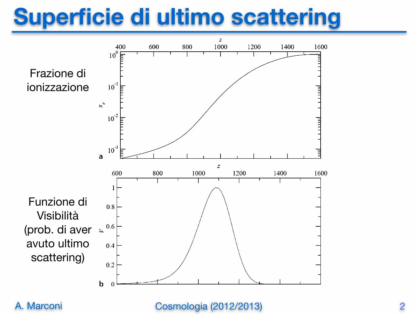
Superficie di ultimo scattering

2

424 15 Fluctuations in the Cosmic Microwave Background Radiation

Fig. 15.1. a Ionisation fraction xe = Ne/NH as a function of redshift z for the WMAPconcordance values for cosmological parameters. b Visibility function v(z) = e!! d!/dznormalised to unity at maximum (Chluba and Sunyaev, 2006)

15.2 The Physical and Angular Scales of the Fluctuations

It is helpful to begin by listing the various scales and dimensions which will appearin the analysis which follows. For the sake of definiteness, we continue to use ourreference set of parameters: "0 = 0.3, "# = 0.7, "B = 0.05, h = 0.7. Wherenecessary, we will use the spectral index n = 1 for the initial power spectrum.The element of comoving radial distance coordinate at redshift z during the matter-dominated era is given by (7.73):

dr = c dz

H0!(1 + z)2("0z + 1) ! "#z(z + 2)

"1/2 , (15.3)

which can be written

dr = c dz

H0!"0(1 + z)3 + "#

"1/2 , (15.4)

if "0 + "# = 1. Strictly speaking, we should also include in this formula thecontribution of the energy density of photons and neutrinos at this redshift, z = 1090,

Frazione di ionizzazione

Funzione di Visibilità

(prob. di aver avuto ultimo scattering)

A. Marconi Cosmologia (2012/2013))

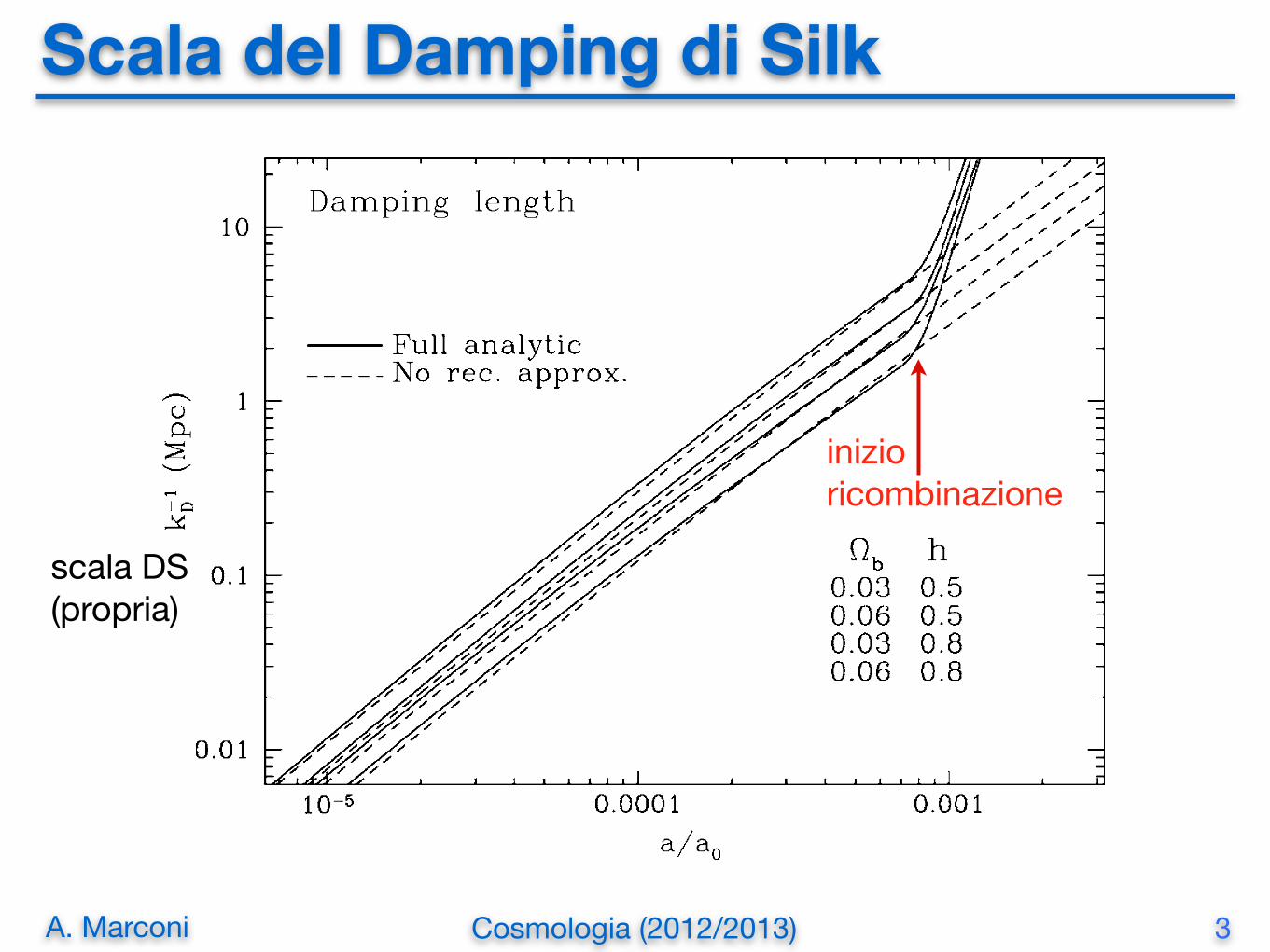
Scala del Damping di Silk

3

426 15 Fluctuations in the Cosmic Microwave Background Radiation

of sight through the last scattering layer. Consequently, the random superposition ofthese perturbations leads to a statistical reduction in the amplitude of the observedintensity fluctuations by a factor of roughly N!1/2, where N is the number offluctuations along the line of sight.

We have already obtained the important result that, for primordial structures onscales greater than those of clusters of galaxies, we observe ‘slices’ through theseon the last scattering layer.

15.2.2 The Silk Damping Scale

Next, we evaluate the comoving damping scale for baryonic perturbations at theepoch of recombination using (12.52) and (12.56) for the case in which the dynamicsof the expansion were determined by the dark matter, t = (2/3H0)!

!1/20 z!1.5,

"S =! 1

3"ct"1/2 = 0.867

!!Bh2

"1/2 !!0h2

"1/4 = 9.0 Mpc . (15.9)

This is a significant underestimate of the damping scale at recombination since ithas not taken account of the dramatic increase in the mean free path of the photonsas the recombination process gets under way. Hu and Sugiyama present a helpfuldiagram showing the impact of reionisation upon the Silk damping length (Fig. 15.2)(Hu and Sugiyama, 1995). Formally the damping scale becomes infinite, but Hu andSugiyama convolve the damping scale with the visibility function so that the dampingscale appropriate for baryonic density perturbations remains finite.

Fig. 15.2. Evolution of the Silk damping scale for primordial density perturbations. Dashedlines: the silk damping length without taking account of recombination. Solid lines: increasein the silk damping length as the process of recombination takes place at z " 1090 (Hu andSugiyama, 1995)

inizioricombinazione

scala DS(propria)

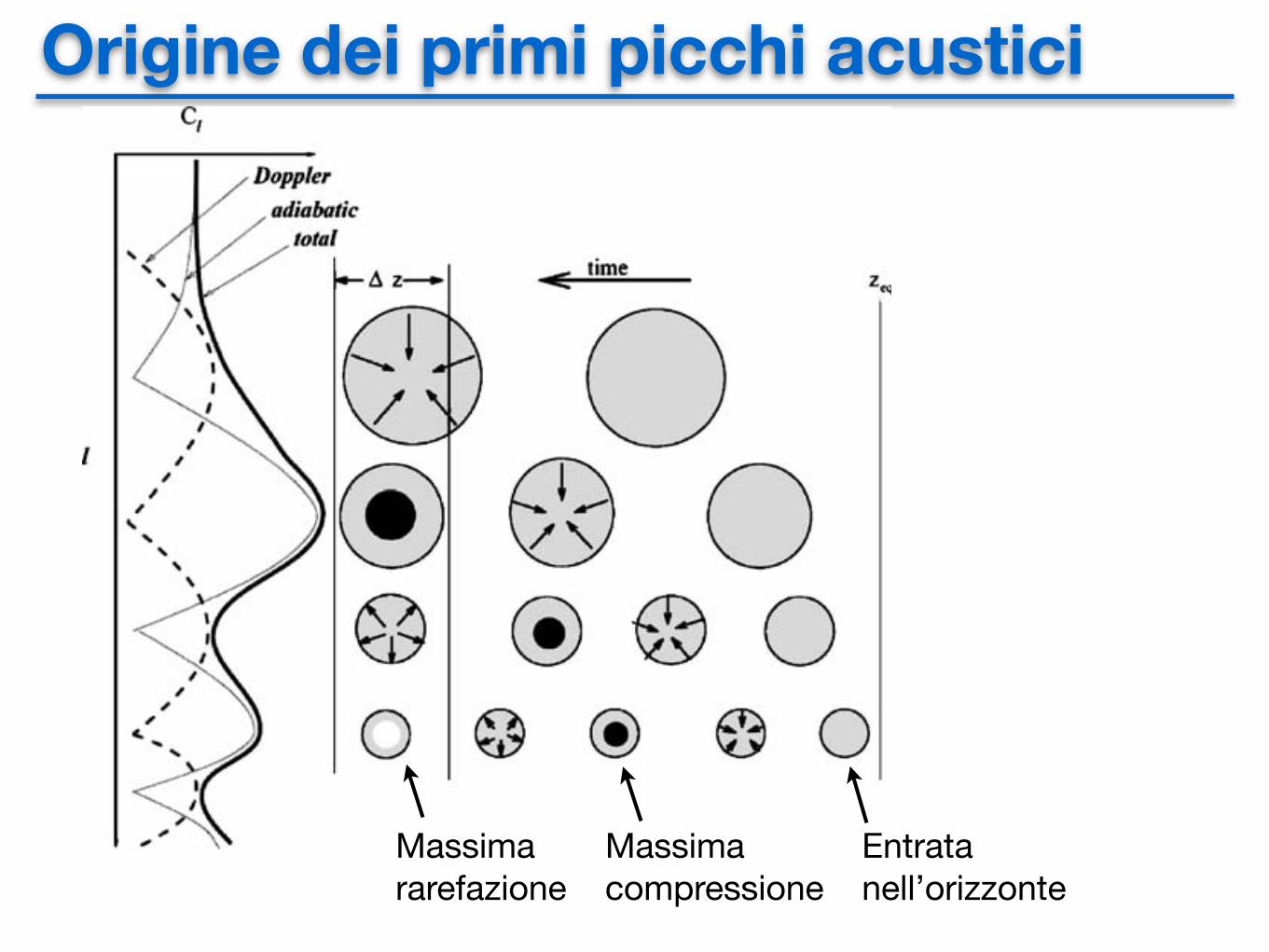
Origine dei primi picchi acustici428 15 Fluctuations in the Cosmic Microwave Background Radiation

Fig. 15.3. Origin of the first few acoustic peaks in the power spectrum of the cosmic mi-crowave background radiation. Circles: the response of the photon-baryon plasma to growingperturbations in cold dark matter potential wells (Lineweaver, 2005). Dark filled circles:maximum compression of the perturbations; white filled circles: maximum of rarefaction ofthe oscillations. zeq is the epoch of equality and !z is the thickness in redshift of the lastscattering layer. Many more details of this diagram are discussed in Sects. 15.4 and 15.5

The second way of thinking about the sound horizon is that it is the maximumcoherence length on the last scattering layer, and so we can work out the expectedangular scale of this acoustic peak in the perturbation spectrum,

!s ! cst(1 + z)D

. (15.14)

For our reference set of cosmological parameters, this angular scale is 0.23". In termsof the angular multipole l on the sky, which is introduced in the next section, thereshould be a maximum in the power spectrum at multipoles of l ! 250, adoptingthe relation l ! !#1

s . Indeed, there is a very pronounced maximum in the powerspectrum at this multipole (Fig. 15.4), but in view of the approximations made inthis derivation, the agreement should be regarded as fortuitous.

The sound horizon is more important than the Jeans length in these studies,but the dispersion relation for baryonic perturbations during the period from theepoch of equality to the epoch of recombination is important. The interpretationof the Jeans length given in Sect. 11.3 was that it is the distance which soundwaves can travel in the free-fall collapse time of the perturbation which is of order" $ (G#)#1/2. The difference between the sound horizon and the Jeans length in

Massima rarefazione

Massima compressione

Entrata nell’orizzonte

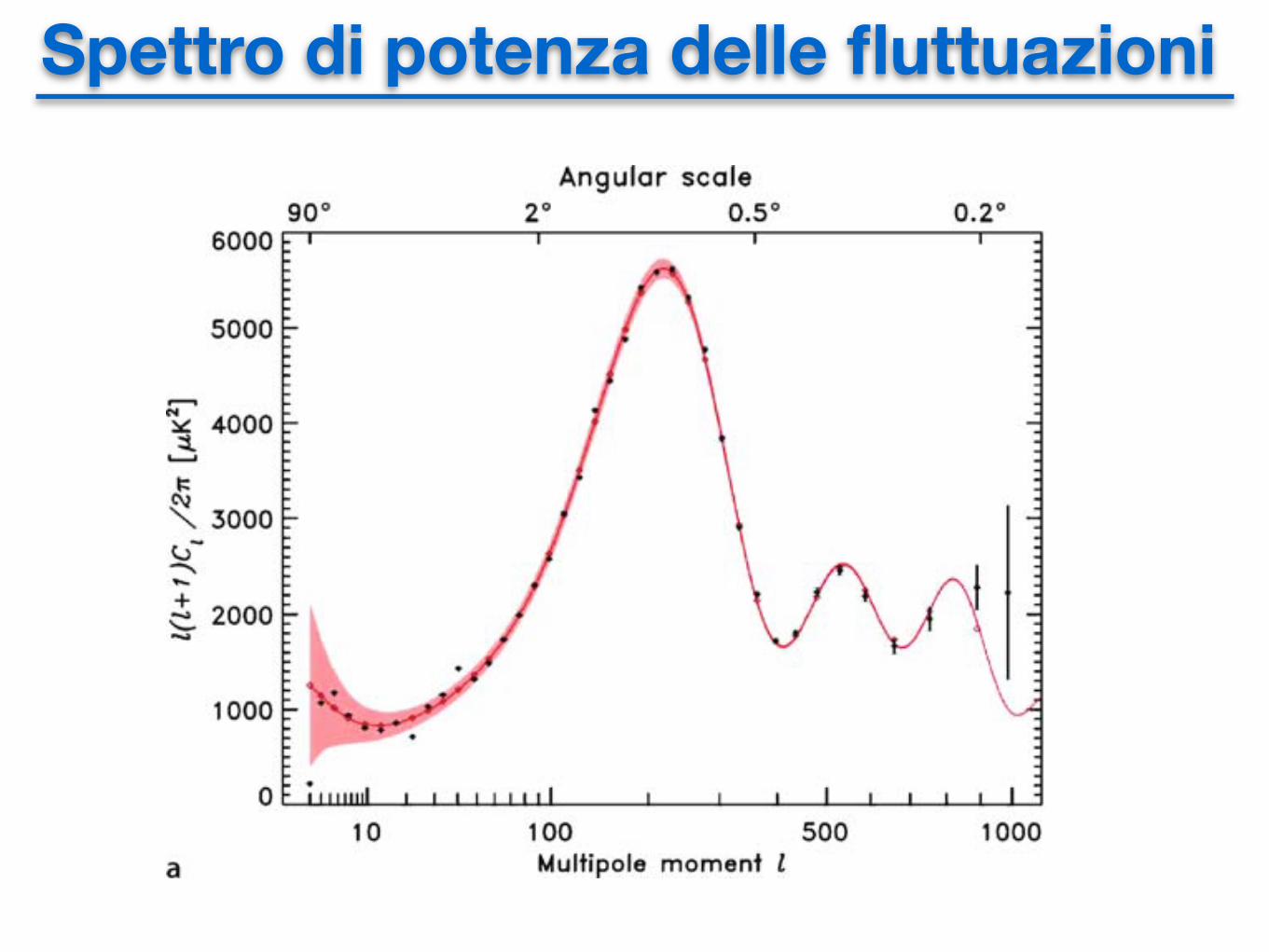
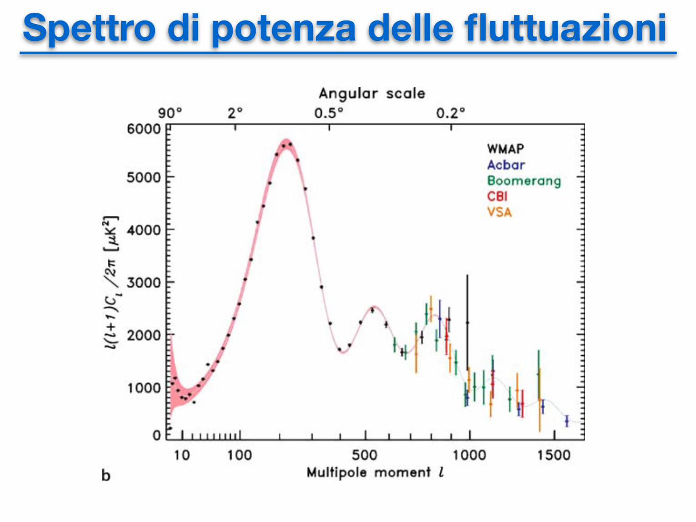
Spettro di potenza delle fluttuazioni15.3 The Power Spectrum of Temperature Fluctuations 435

Fig. 15.4. a The binned 3-year angular power spectrum from the WMAP experiment (blacksymbols with 1 ! ! noise error bars for 2 " l " 1000). The grey band is the binned 1 ! !

cosmic-variance uncertainty (Hinshaw et al., 2007). The curve is the best-fit "CDM model forthe WMAP data alone (Spergel et al., 2007). The diamonds show the model points when binnedin the same way as the data. b The WMAP 3-year power spectrum and other measurementsof the angular power spectrum extending to larger multipole moments (Hinshaw et al., 2007).The additional data, which have been restricted to those at large multipoles, are from theBoomerang (Jones et al., 2006), Acbar (Kuo et al., 2004), CBI (Readhead et al., 2004) andVSA (Dickinson et al., 2004) experiments. In both diagrams, note the variable logarithmicscale in multipole moment along the abscissa

Spettro di potenza delle fluttuazioni

15.3 The Power Spectrum of Temperature Fluctuations 435

Fig. 15.4. a The binned 3-year angular power spectrum from the WMAP experiment (blacksymbols with 1 ! ! noise error bars for 2 " l " 1000). The grey band is the binned 1 ! !

cosmic-variance uncertainty (Hinshaw et al., 2007). The curve is the best-fit "CDM model forthe WMAP data alone (Spergel et al., 2007). The diamonds show the model points when binnedin the same way as the data. b The WMAP 3-year power spectrum and other measurementsof the angular power spectrum extending to larger multipole moments (Hinshaw et al., 2007).The additional data, which have been restricted to those at large multipoles, are from theBoomerang (Jones et al., 2006), Acbar (Kuo et al., 2004), CBI (Readhead et al., 2004) andVSA (Dickinson et al., 2004) experiments. In both diagrams, note the variable logarithmicscale in multipole moment along the abscissa

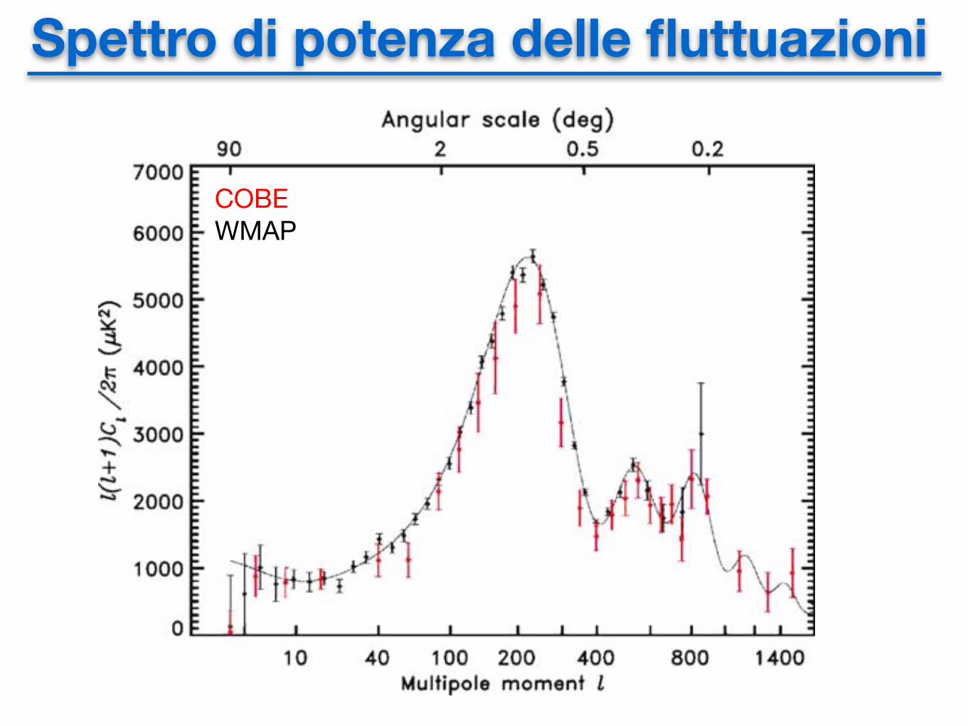
Spettro di potenza delle fluttuazioni15.4 Large Angular Scales 437

Fig. 15.5. The WMAP power spectrum from the first year of observation, compared withdata published prior to WMAP, including COBE. The WMAP data are plotted with cosmicvariance plus measurement uncertainties. The COBE and WMAP power spectra are in goodagreement (Hinshaw et al., 2003)

The most straightforward way of approaching the problem is to use (13.9), whichrelates the curvature perturbations on superhorizon scales to the density contrasts inthe baryonic matter, the cold dark matter and the radiation,

13

!"B

"B= 1

3!"D

"D= 1

4!"rad

"rad. (15.31)

Since "rad = aT 4, it follows that

!TT

= 13

!"D

"D. (15.32)

We can illustrate the origin of this relation by a simple Newtonian argument whichalso shows how the issue of the choice of gauge enters the problem. According tothe ‘Newtonian’ argument which led to (6.8), for small gravitational perturbationsthe frequency shift and the corresponding change in the thermodynamic temperatureof the background radiation can be related to the gravitational redshift zgrav

!#

#= !T

T= zgrav = !$

c2. (15.33)

This result is different from that found in a general relativistic treatment becausewe also need to take account of the time dilation of the radiation as it climbs out of

COBEWMAP

Spettro di PlanckPlanck collaboration: CMB power spectra & likelihood

2 10 500

1000

2000

3000

4000

5000

6000

D�[µK

2 ]

90� 18�

500 1000 1500 2000 2500

Multipole moment, �

1� 0.2� 0.1� 0.07�Angular scale

Figure 37. The 2013 Planck CMB temperature angular power spectrum. The error bars include cosmic variance, whose magnitudeis indicated by the green shaded area around the best fit model. The low-` values are plotted at 2, 3, 4, 5, 6, 7, 8, 9.5, 11.5, 13.5, 16,19, 22.5, 27, 34.5, and 44.5.

Table 8. Constraints on the basic six-parameter ⇤CDM model using Planck data. The top section contains constraints on the sixprimary parameters included directly in the estimation process, and the bottom section contains constraints on derived parameters.

Planck Planck+WP

Parameter Best fit 68% limits Best fit 68% limits

⌦bh2 . . . . . . . . . 0.022068 0.02207 ± 0.00033 0.022032 0.02205 ± 0.00028

⌦ch2 . . . . . . . . . 0.12029 0.1196 ± 0.0031 0.12038 0.1199 ± 0.0027100✓MC . . . . . . . 1.04122 1.04132 ± 0.00068 1.04119 1.04131 ± 0.00063

⌧ . . . . . . . . . . . . 0.0925 0.097 ± 0.038 0.0925 0.089+0.012�0.014

ns . . . . . . . . . . . 0.9624 0.9616 ± 0.0094 0.9619 0.9603 ± 0.0073

ln(1010As) . . . . . 3.098 3.103 ± 0.072 3.0980 3.089+0.024�0.027

⌦⇤ . . . . . . . . . . 0.6825 0.686 ± 0.020 0.6817 0.685+0.018�0.016

⌦m . . . . . . . . . . 0.3175 0.314 ± 0.020 0.3183 0.315+0.016�0.018

�8 . . . . . . . . . . . 0.8344 0.834 ± 0.027 0.8347 0.829 ± 0.012

zre . . . . . . . . . . . 11.35 11.4+4.0�2.8 11.37 11.1 ± 1.1

H0 . . . . . . . . . . 67.11 67.4 ± 1.4 67.04 67.3 ± 1.2

109As . . . . . . . . 2.215 2.23 ± 0.16 2.215 2.196+0.051�0.060

⌦mh2 . . . . . . . . . 0.14300 0.1423 ± 0.0029 0.14305 0.1426 ± 0.0025Age/Gyr . . . . . . 13.819 13.813 ± 0.058 13.8242 13.817 ± 0.048z⇤ . . . . . . . . . . . 1090.43 1090.37 ± 0.65 1090.48 1090.43 ± 0.54100✓⇤ . . . . . . . . 1.04139 1.04148 ± 0.00066 1.04136 1.04147 ± 0.00062zeq . . . . . . . . . . . 3402 3386 ± 69 3403 3391 ± 60

33

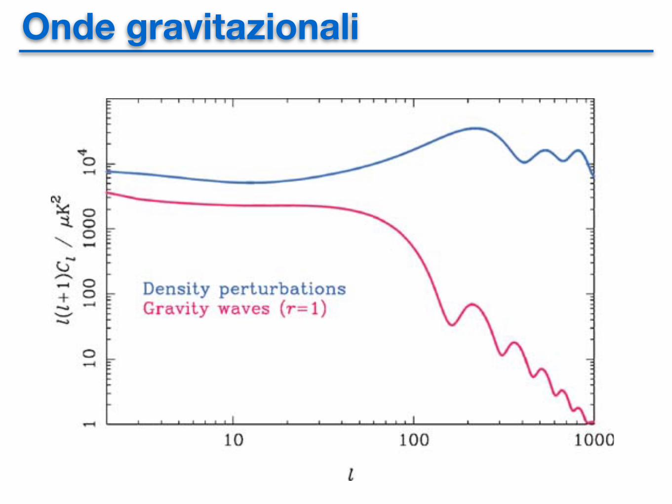
Onde gravitazionali442 15 Fluctuations in the Cosmic Microwave Background Radiation

Fig. 15.6. The predicted power spectra of fluctuations in the cosmic microwave backgroundradiation due to scalar perturbations (density perturbations; top) and tensor perturbations(gravity waves; bottom) for a tensor-to-scalar ratio r = 1 (Challinor, 2005)

upon the form of the inflationary potential (Starobinsky, 1985; Davis et al., 1992b;Crittenden et al., 1993). According to these theories, the ratio of the power spectradepends upon the spectral index of the scalar perturbations as

!2T

!2s

! 6(1 " n) , (15.41)

where !2T and !2

s are the density perturbations in the tensor and scalar modesrespectively. Peacock provides an accessible introduction to this topic (Peacock,2000). Thus, an important test of inflation is to measure the spectral index n ofthe scalar power spectrum with high precision, and this is now possible with theavailability of the 3-year WMAP data set. To summarise the findings, which aredealt with in more detail in Sect. 15.9, the best-fit value of n to all the observationaldata is n = 0.951+0.015

"0.019 , suggesting that the predicted ‘tilt’ of the power spectrummay have been observed (Spergel et al., 2007).

We can set limits to the energy density of primordial gravitational waves at thepresent epoch from the observed power spectrum of the COBE fluctuations. Aspointed out by Padmanabhan, gravitational waves at the present epoch with wave-length " # c/H0 would produce a quadrupole anisotropy in the cosmic microwavebackground radiation through the Sachs–Wolfe effect, and so the upper limit to theamplitude of these waves is the quadrupole anisotropy h # !T/T ! 10"5 (Padman-abhan, 1993). Therefore, the upper limit to the energy density of these gravitationalwaves is

#G = $Gc2 # (32%G)"1 !&2h2c2" , (15.42)

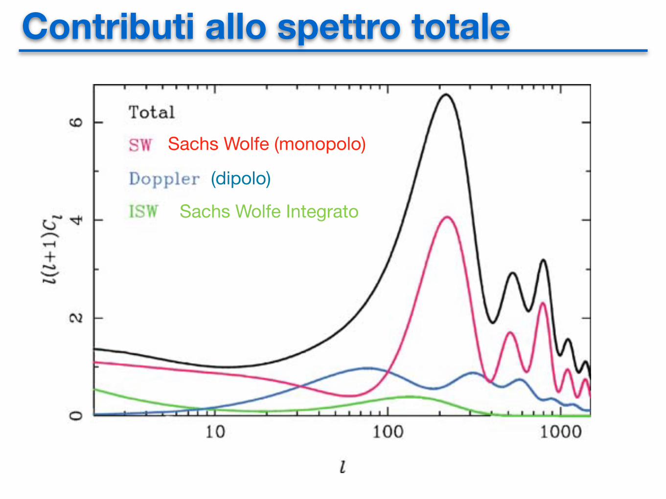
Contributi allo spettro totale456 15 Fluctuations in the Cosmic Microwave Background Radiation

Fig. 15.9. Contributions of various terms to the temperature anisotropy power spectrum foradiabatic initial density perturbations. At large values of l, the contributions are, (top tobottom): total power; SW, the Sachs–Wolfe effect including the monopole anisotropy; theDoppler or dipole term; the integrated Sachs–Wolfe effect (Challinor, 2005)

As a result, the polarisation signal is expected to be much weaker than theintensity fluctuations. It is therefore a very considerable challenge to measure thepolarisation signal experimentally, but this was first achieved by the ground-basedDegree Angular Scale Interferometer (DASI) in 2002 (Leitch et al., 2002; Kovacet al., 2002). Subsequent ground-based experiments including the CBI (Readheadet al., 2004), the CAPMAP (Barkats et al., 2005) and Boomerang (Montroy et al.,2006) projects reported convincing detections of the polarised background signal.5

From space, the WMAP experiment detected a positive polarisation signal in the1-year data (Bennett et al., 2003) and this was confirmed with improved signal-to-noise ratio in the 3-year data release (Page et al., 2007). It is simplest to summarisethe results of these efforts using the 3-year WMAP polarisation data. It is againappropriate to pay tribute to the outstanding experimental and data analysis skillswhich have gone into these extremely demanding experiments. The extraction ofthe polarisation signal is particularly challenging because it has to be detected in thepresence of the polarised Galactic radio emission, which has to be removed from thesky maps to reveal the polarisation associated with the primordial perturbations.

The total intensity fluctuations which were shown in Fig. 15.3 are displayedas filled dots at the top of Fig. 15.10 and are labelled TT. The polarisation powerspectrum is labelled EE. The oscillating curve, which decreases towards small mul-

5 The reader by now will be aware of my preference to avoid acronyms but I have par-tially capitulated here: the translations are as follows: CBI = Cosmic Background Imager;CAPMAP = Cosmic Anisotropy Polarization Mapper; BOOMERanG = Balloon Observa-tions Of Millimetric Extragalactic Radiation ANisotropy and Geophysics.

Sachs Wolfe (monopolo)

Sachs Wolfe Integrato

(dipolo)

Spettro di potenza CMB

15.5 Intermediate Angular Scales – the Acoustic Peaks 449

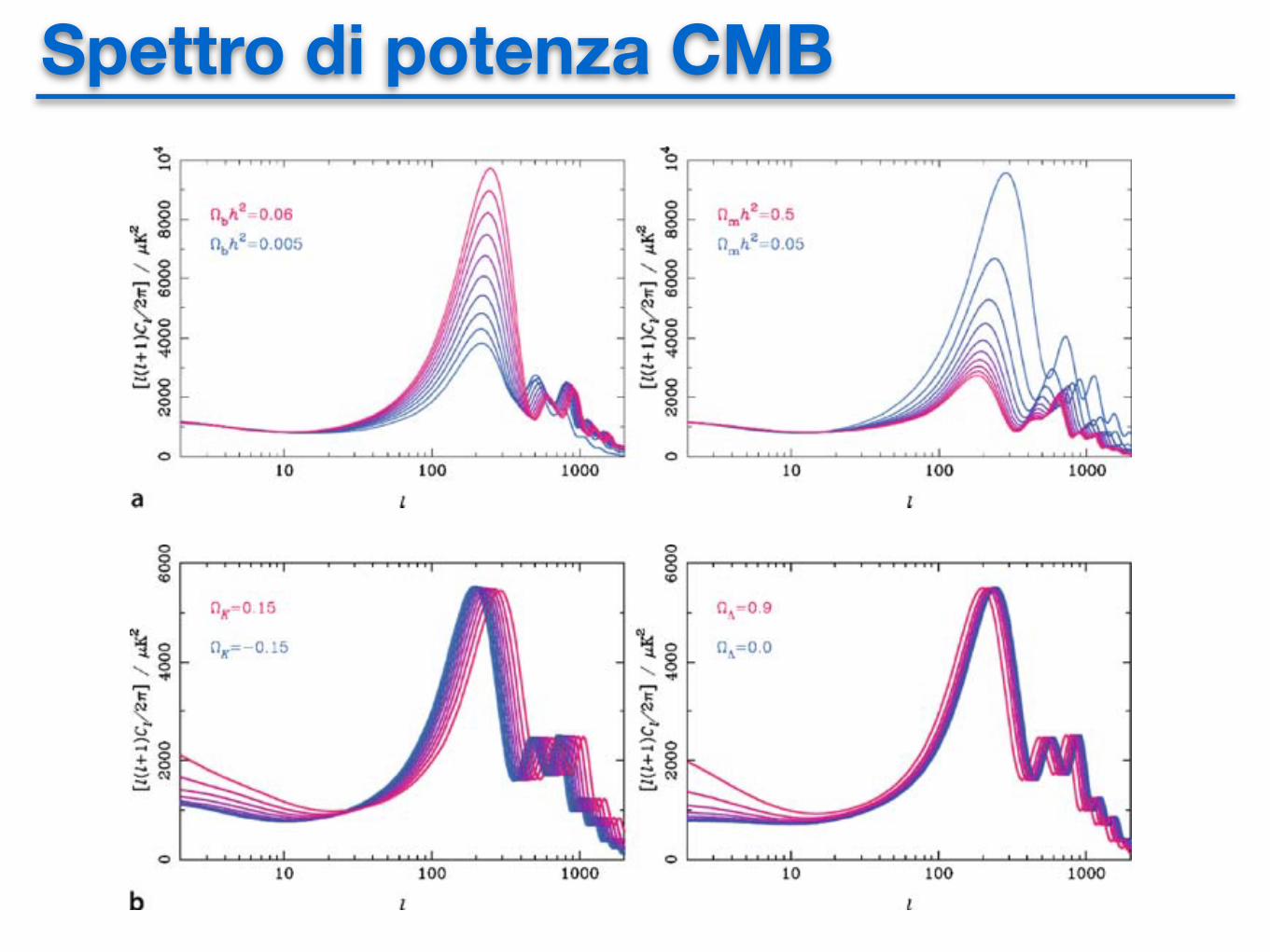
Some examples of the results of detailed predictions by Challinor are shown inFig. 15.7, indicating how different features of the temperature anisotropy powerspectrum are sensitive to variations of the cosmological parameters (Challinor, 2005).It is a useful exercise to study the power spectra in Fig. 15.7 in some detail and touse the results we have established in this section to understand the dependencesupon cosmological parameters. For example, the left-hand plot of Fig. 15.7a showsclearly the strong enhancement of the first acoustic peak as the baryon densityincreases.

Fig. 15.7a,b. The dependence of the temperature-anisotropy power spectrum on differentcosmological parameters (Challinor, 2005). In these examples, scale-invariant adiabatic initialperturbations are assumed. a Top pair of diagrams: dependence on the density parameter inbaryons (left) and total matter density parameter !0 (right). Top to bottom at first peak: thebaryon density parameter varies linearly in the range 0.06 ! !Bh2 ! 0.005 (left) and thematter density parameter in the range 0.05 " !Bh2 " 0.5 (right). b Bottom pair of diagrams:The dependence on the curvature density parameter !" (left) and the dark energy densityparameter !# (right). In both cases, the density parameters in baryons and matter were heldconstant, thus preserving the conditions on the last scattering layer. The curvature densityparameter varies (left to right) in the range #0.15 " !" " 0.15 and the dark matter densityparameter in the range 0.9 ! !# ! 0.0

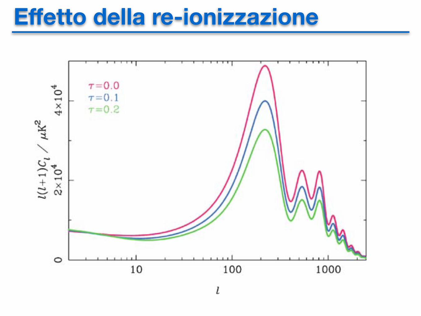
Effetto della re-ionizzazione15.7 The Reionised Intergalactic Gas 453

Fig. 15.8. The effect of reionisation on the temperature anisotropy power spectrum. Thespectra are (top to bottom) for no reionisation, ! = 0.1 and 0.2. (Challinor, 2005)

reionised, presumably by the earliest generations of massive stars. These redshiftsare not unreasonable values, as we will discuss in more detail in Chap. 18. Theoptical depth for Thomson scattering is one of the key cosmological parameters tobe found from detailed analysis of the observed power spectrum of fluctuations inthe cosmic microwave background radiation.

The formation of early generations of objects would necessarily give rise tosignificant velocity perturbations during the reionisation epoch, resulting in Dopplershifts of the background radiation, in exactly the same way that the dipole temperatureperturbations were generated at the last scattering layer. The problem is that theseeffects are expected to be small, partly because the optical depth of the perturbationsis small, and also because the random superposition of these perturbations leads toa statistical decrease of their amplitude. There is, however, a second-order effectdiscussed by Vishniac which does not lead to the statistical cancellation of thevelocity perturbations (Vishniac, 1987). These perturbations are associated withsecond-order terms in "nev, where "ne is the perturbation in the electron density andv the peculiar velocity associated with the motion of the perturbation. This effectonly becomes significant on small angular scales at which the density perturbationsare large. According to Vishniac’s calculations, in the standard cold dark matterpicture, these temperature fluctuations might amount to !T/T ! 10"5 on the scale of1 arcmin. Similar calculations have been carried out by Efstathiou with essentially thesame result (Efstathiou, 1988). These are important conclusions since it is expectedthat all primordial perturbations on these scales would have been damped out by theprocesses discussed in Sect. 15.6.1.

Contributi allo spettro totale456 15 Fluctuations in the Cosmic Microwave Background Radiation

Fig. 15.9. Contributions of various terms to the temperature anisotropy power spectrum foradiabatic initial density perturbations. At large values of l, the contributions are, (top tobottom): total power; SW, the Sachs–Wolfe effect including the monopole anisotropy; theDoppler or dipole term; the integrated Sachs–Wolfe effect (Challinor, 2005)

As a result, the polarisation signal is expected to be much weaker than theintensity fluctuations. It is therefore a very considerable challenge to measure thepolarisation signal experimentally, but this was first achieved by the ground-basedDegree Angular Scale Interferometer (DASI) in 2002 (Leitch et al., 2002; Kovacet al., 2002). Subsequent ground-based experiments including the CBI (Readheadet al., 2004), the CAPMAP (Barkats et al., 2005) and Boomerang (Montroy et al.,2006) projects reported convincing detections of the polarised background signal.5

From space, the WMAP experiment detected a positive polarisation signal in the1-year data (Bennett et al., 2003) and this was confirmed with improved signal-to-noise ratio in the 3-year data release (Page et al., 2007). It is simplest to summarisethe results of these efforts using the 3-year WMAP polarisation data. It is againappropriate to pay tribute to the outstanding experimental and data analysis skillswhich have gone into these extremely demanding experiments. The extraction ofthe polarisation signal is particularly challenging because it has to be detected in thepresence of the polarised Galactic radio emission, which has to be removed from thesky maps to reveal the polarisation associated with the primordial perturbations.

The total intensity fluctuations which were shown in Fig. 15.3 are displayedas filled dots at the top of Fig. 15.10 and are labelled TT. The polarisation powerspectrum is labelled EE. The oscillating curve, which decreases towards small mul-

5 The reader by now will be aware of my preference to avoid acronyms but I have par-tially capitulated here: the translations are as follows: CBI = Cosmic Background Imager;CAPMAP = Cosmic Anisotropy Polarization Mapper; BOOMERanG = Balloon Observa-tions Of Millimetric Extragalactic Radiation ANisotropy and Geophysics.

Sachs Wolfe (monopolo)

Sachs Wolfe Integrato

(dipolo)

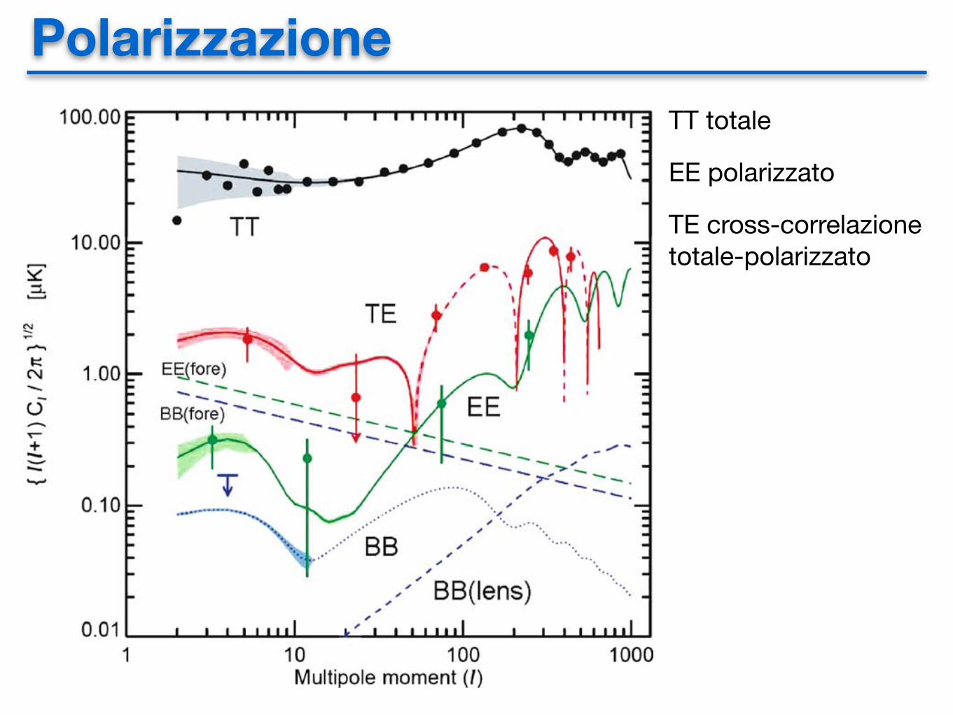
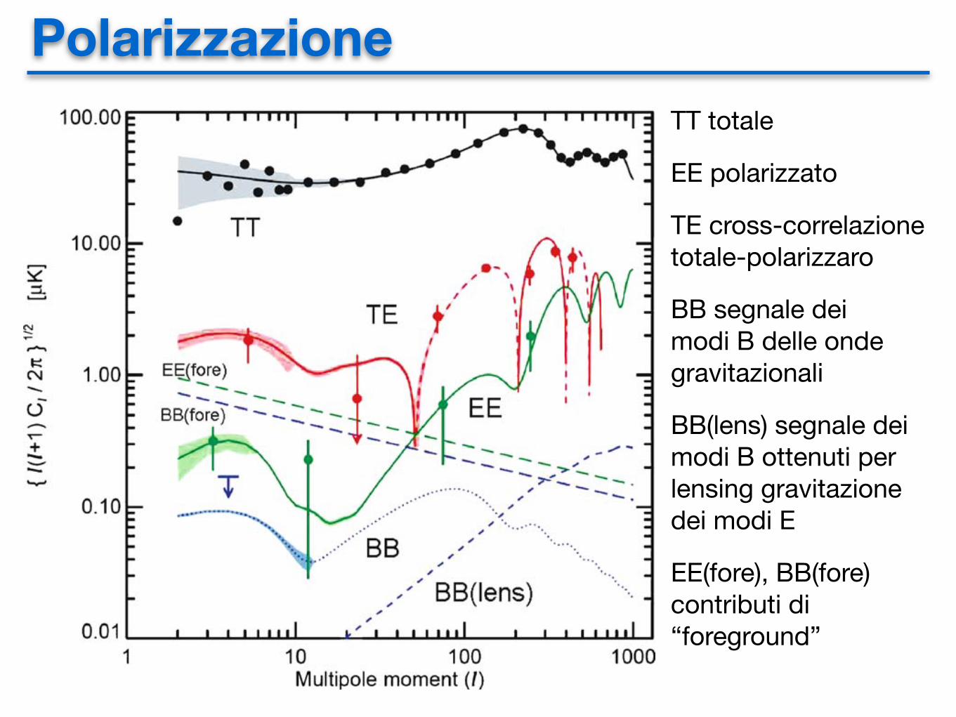
Polarizzazione15.8 The Polarisation of the Cosmic Microwave Background Radiation 457

Fig. 15.10. The measured power spectrum of fluctuations in the intensity and polarisationof the cosmic microwave background radiation. Plots for the total intensity, the polarisedintensity and the cross-correlation between the total intensity and the polarised intensity arelabelled TT, EE and TE respectively. The best fitting model is shown by the correspondinglines. The dashed sections of the TE curve indicates multipoles in which the polarisationsignal is anticorrelated with the total intensity. The model predictions are binned in l in thesame way as the data. The binned EE polarisation data are divided into bins of 2 ! l ! 5,6 ! l ! 49, 50 ! l ! 199, and 200 ! l ! 799. The dotted line labelled BB shows theexpected power spectrum of B-mode gravitational waves if the primordial ratio of tensorto scalar perturbations was r = !2

t /!2s = 0.3. The WMAP experiment found only upper

limits to this signal, the 1" upper limit corresponding to 0.17 µK for the weighted average ofmultipoles l = 2–10. The B-mode signal due to gravitational lensing of the E-modes is shownas a dashed line labelled BB(lens). The upturn in the polarised signal at l ! 10 is associatedwith polarisation originating during the reionisation era. The foreground model for galacticsynchrotron radiation plus dust emission is shown as straight dashed lines labelled EE(fore)and BB(fore) for the scalar and tensor modes respectively, both being evaluated at # = 65GHz (Page et al., 2007)

TT totale

EE polarizzato

TE cross-correlazione totale-polarizzato

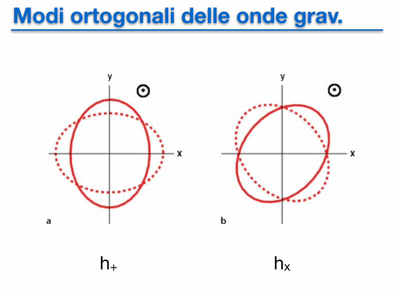
Modi ortogonali delle onde grav.

15.8 The Polarisation of the Cosmic Microwave Background Radiation 459

by differentiation and this is the cause of the quadrupole component responsible forthe generation of the linearly polarised signal. This procedure is repeated for the latereionisation phases and accounts for the predicted linear polarisation ‘bump’ seenin the EE and TE power spectra in Fig. 15.10. Page and his colleagues point outthat these polarisation observations provide entirely independent information aboutthe optical depth for reionisation and consequently about the epoch at which it tookplace (Page et al., 2007).

15.8.4 Primordial Gravitational Waves

The considerations of Sect. 15.8.1 make it clear that gravitational waves can resultin polarisation of the cosmic microwave background radiation. Because the force ofgravity is always attractive, there are no dipole gravitational waves, only quadrupolewaves.6 As a result, gravitational waves stretch and squeeze the geometry of spacein orthogonal directions, the two independent modes of oscillation, h+ and h!,being shown in Fig. 15.11 – they are oriented at 45" with respect to one another.There is, however, an important difference between the two modes in that theyhave opposite parity on making the translation r # $r. The net result is that thepolarisation signal can be uniquely decomposed into what are known as the electricE, or gradient, component associated with h+ and a magnetic B, or curl, componentwith h!. These result in corresponding orthogonal patterns of polarisation on thesky. The importance of this decomposition is that, whereas the E components couldbe generated by either scalar or tensor perturbations, the B component is a signatureof the presence of a pure curl component.

The importance of these considerations is that they provide another potentialmeans of investigating physical processes in the very early Universe. Just as thespectrum of scalar perturbations can be associated with quantum fluctuations of the

Fig. 15.11a,b. The two orthogonal polarisation modes, h+ and h!, of gravitational radiation(Will, 2006)

6 For a simple introduction to gravitational radiation, see the review by Schutz (Schutz,2001).

h+ hx

Polarizzazione15.8 The Polarisation of the Cosmic Microwave Background Radiation 457

Fig. 15.10. The measured power spectrum of fluctuations in the intensity and polarisationof the cosmic microwave background radiation. Plots for the total intensity, the polarisedintensity and the cross-correlation between the total intensity and the polarised intensity arelabelled TT, EE and TE respectively. The best fitting model is shown by the correspondinglines. The dashed sections of the TE curve indicates multipoles in which the polarisationsignal is anticorrelated with the total intensity. The model predictions are binned in l in thesame way as the data. The binned EE polarisation data are divided into bins of 2 ! l ! 5,6 ! l ! 49, 50 ! l ! 199, and 200 ! l ! 799. The dotted line labelled BB shows theexpected power spectrum of B-mode gravitational waves if the primordial ratio of tensorto scalar perturbations was r = !2

t /!2s = 0.3. The WMAP experiment found only upper

limits to this signal, the 1" upper limit corresponding to 0.17 µK for the weighted average ofmultipoles l = 2–10. The B-mode signal due to gravitational lensing of the E-modes is shownas a dashed line labelled BB(lens). The upturn in the polarised signal at l ! 10 is associatedwith polarisation originating during the reionisation era. The foreground model for galacticsynchrotron radiation plus dust emission is shown as straight dashed lines labelled EE(fore)and BB(fore) for the scalar and tensor modes respectively, both being evaluated at # = 65GHz (Page et al., 2007)

TT totale

EE polarizzato

TE cross-correlazione totale-polarizzaro

BB segnale dei modi B delle onde gravitazionali

BB(lens) segnale dei modi B ottenuti per lensing gravitazione dei modi E

EE(fore), BB(fore) contributi di “foreground”

Parametri cosmologici• h = (H0/100 km s!1 Mpc!1)

• !b = !bh2, the baryon density parameter

• !d = !dh2 dark matter density parameter

• !" = dark energy density parameter

• w = dark energy equation of state, p = w"c2 (w = !1 ”prefered”)

• # = reionisation optical depth

• !K = space curvature, recalling that !m + !" + !K = 1

• As = amplitude of scalar power-spectrum

• ns = scalar spectral index; ns = 1 preferred

• a = running of scalar spectral index

• r = tensor-scalar ratio

• nt = tensor spectral index

• b = bias factor

• fn = neutrino fraction Show simulations

36

Spettro di potenza CMB

15.5 Intermediate Angular Scales – the Acoustic Peaks 449

Some examples of the results of detailed predictions by Challinor are shown inFig. 15.7, indicating how different features of the temperature anisotropy powerspectrum are sensitive to variations of the cosmological parameters (Challinor, 2005).It is a useful exercise to study the power spectra in Fig. 15.7 in some detail and touse the results we have established in this section to understand the dependencesupon cosmological parameters. For example, the left-hand plot of Fig. 15.7a showsclearly the strong enhancement of the first acoustic peak as the baryon densityincreases.

Fig. 15.7a,b. The dependence of the temperature-anisotropy power spectrum on differentcosmological parameters (Challinor, 2005). In these examples, scale-invariant adiabatic initialperturbations are assumed. a Top pair of diagrams: dependence on the density parameter inbaryons (left) and total matter density parameter !0 (right). Top to bottom at first peak: thebaryon density parameter varies linearly in the range 0.06 ! !Bh2 ! 0.005 (left) and thematter density parameter in the range 0.05 " !Bh2 " 0.5 (right). b Bottom pair of diagrams:The dependence on the curvature density parameter !" (left) and the dark energy densityparameter !# (right). In both cases, the density parameters in baryons and matter were heldconstant, thus preserving the conditions on the last scattering layer. The curvature densityparameter varies (left to right) in the range #0.15 " !" " 0.15 and the dark matter densityparameter in the range 0.9 ! !# ! 0.0

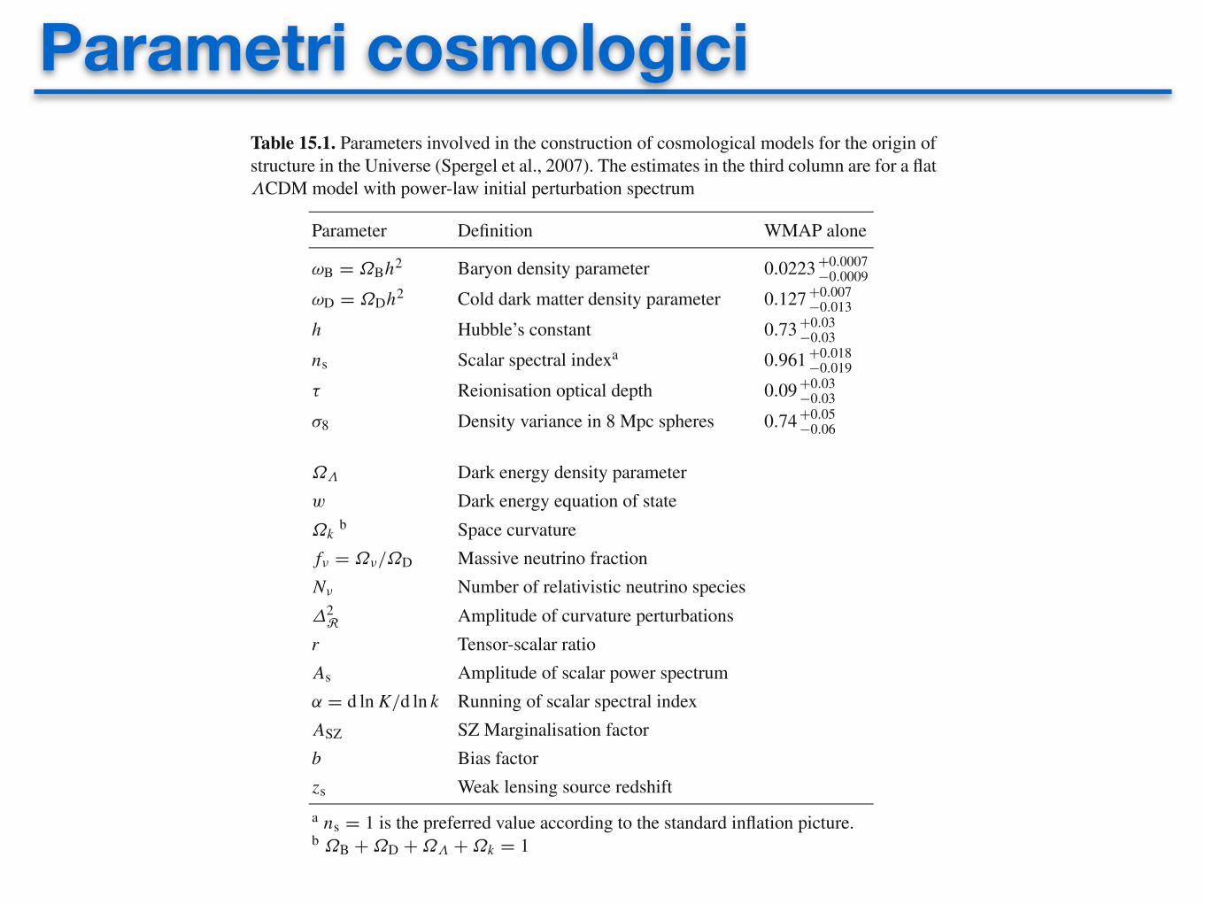
Parametri cosmologici464 15 Fluctuations in the Cosmic Microwave Background Radiation

Table 15.1. Parameters involved in the construction of cosmological models for the origin ofstructure in the Universe (Spergel et al., 2007). The estimates in the third column are for a flat!CDM model with power-law initial perturbation spectrum

Parameter Definition WMAP alone

"B = #Bh2 Baryon density parameter 0.0223 +0.0007!0.0009

"D = #Dh2 Cold dark matter density parameter 0.127 +0.007!0.013

h Hubble’s constant 0.73 +0.03!0.03

ns Scalar spectral indexa 0.961 +0.018!0.019

$ Reionisation optical depth 0.09 +0.03!0.03

%8 Density variance in 8 Mpc spheres 0.74 +0.05!0.06

#! Dark energy density parameter

w Dark energy equation of state

#kb Space curvature

f& = #&/#D Massive neutrino fraction

N& Number of relativistic neutrino species

'2R Amplitude of curvature perturbations

r Tensor-scalar ratio

As Amplitude of scalar power spectrum

( = d ln K/d ln k Running of scalar spectral index

ASZ SZ Marginalisation factor

b Bias factor

zs Weak lensing source redshift

a ns = 1 is the preferred value according to the standard inflation picture.b #B + #D + #! + #k = 1

spectrum. Blank entries in the table mean that they were set to zero or their valuescould be deduced from the first six quantities and the assumption of a flat !CDMmodel.

It is remarkable how closely these values agree with the completely independentestimates of these parameters which were discussed in Chap. 8. Particularly strikingresults are:

– The dark energy density parameter #! " 0.7 while the dark matter has densityparameter #Dh2 " 0.127, both in excellent agreement with the estimates fromType 1A supernovae (Sect. 8.5.3) and from large-scale galaxy surveys (Sect. 8.7).

– The baryonic matter has density parameter #Bh2 " 0.0223, in excellent agree-ment with the results of primordial nucleosynthesis (Sect. 10.4.2).

– The inferred value of Hubble’s constant is in excellent agreement with the resultsof the Hubble Space Telescope Key Project (Sect. 8.3).

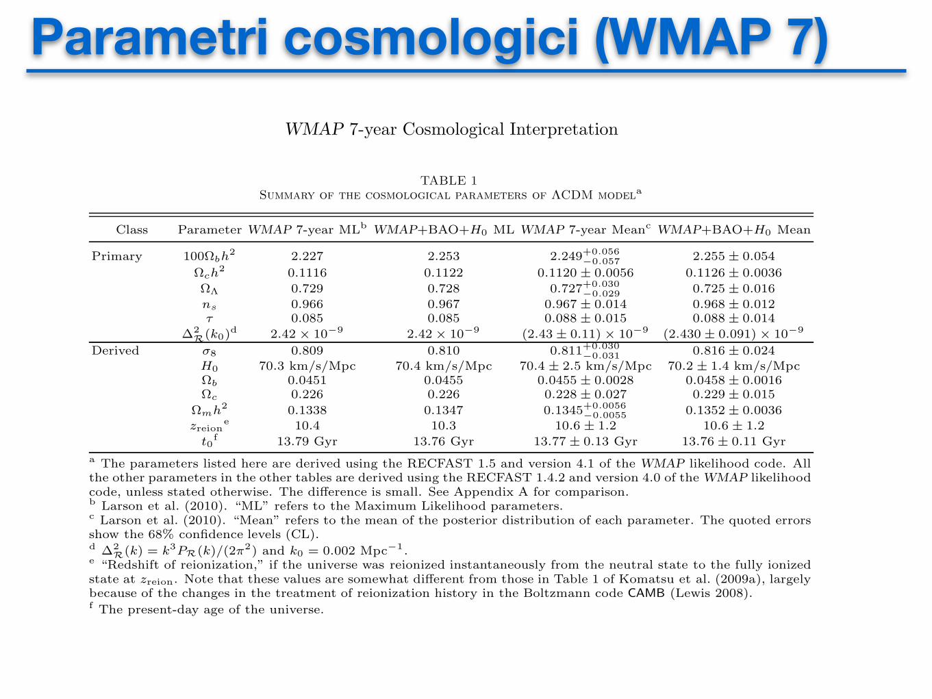
Parametri cosmologici (WMAP 7)WMAP 7-year Cosmological Interpretation 3

TABLE 1Summary of the cosmological parameters of !CDM modela

Class Parameter WMAP 7-year MLbWMAP+BAO+H0 ML WMAP 7-year Meanc

WMAP+BAO+H0 Mean

Primary 100"bh2 2.227 2.253 2.249+0.056

!0.057 2.255 ± 0.054

"ch2 0.1116 0.1122 0.1120 ± 0.0056 0.1126 ± 0.0036

"! 0.729 0.728 0.727+0.030!0.029 0.725 ± 0.016

ns 0.966 0.967 0.967 ± 0.014 0.968 ± 0.012! 0.085 0.085 0.088 ± 0.015 0.088 ± 0.014

#2R(k0)

d 2.42 ! 10!9 2.42 ! 10!9 (2.43 ± 0.11) ! 10!9 (2.430 ± 0.091) ! 10!9

Derived "8 0.809 0.810 0.811+0.030!0.031 0.816 ± 0.024

H0 70.3 km/s/Mpc 70.4 km/s/Mpc 70.4 ± 2.5 km/s/Mpc 70.2 ± 1.4 km/s/Mpc"b 0.0451 0.0455 0.0455 ± 0.0028 0.0458 ± 0.0016"c 0.226 0.226 0.228 ± 0.027 0.229 ± 0.015

"mh2 0.1338 0.1347 0.1345+0.0056!0.0055 0.1352 ± 0.0036

zreione 10.4 10.3 10.6 ± 1.2 10.6 ± 1.2

t0f 13.79 Gyr 13.76 Gyr 13.77 ± 0.13 Gyr 13.76 ± 0.11 Gyr

a The parameters listed here are derived using the RECFAST 1.5 and version 4.1 of the WMAP likelihood code. Allthe other parameters in the other tables are derived using the RECFAST 1.4.2 and version 4.0 of the WMAP likelihoodcode, unless stated otherwise. The di$erence is small. See Appendix A for comparison.b Larson et al. (2010). “ML” refers to the Maximum Likelihood parameters.c Larson et al. (2010). “Mean” refers to the mean of the posterior distribution of each parameter. The quoted errorsshow the 68% confidence levels (CL).d #2

R(k) = k3PR(k)/(2#2) and k0 = 0.002 Mpc!1.e “Redshift of reionization,” if the universe was reionized instantaneously from the neutral state to the fully ionizedstate at zreion. Note that these values are somewhat di$erent from those in Table 1 of Komatsu et al. (2009a), largelybecause of the changes in the treatment of reionization history in the Boltzmann code CAMB (Lewis 2008).f The present-day age of the universe.

TABLE 2Summary of the 95% confidence limits on deviations from the simple (flat, Gaussian, adiabatic, power-law) !CDM model except for dark energy

parameters

Section Name Case WMAP 7-year WMAP+BAO+SNaWMAP+BAO+H0

Section 4.1 Grav. Waveb No Running Ind. r < 0.36c r < 0.20 r < 0.24Section 4.2 Running Index No Grav. Wave "0.084 < dns/d ln k < 0.020c "0.065 < dns/d ln k < 0.010 "0.061 < dns/d lnk < 0.017Section 4.3 Curvature w = "1 N/A "0.0178 < "k < 0.0063 "0.0133 < "k < 0.0084Section 4.4 Adiabaticity Axion $0 < 0.13c $0 < 0.064 $0 < 0.077

Curvaton $!1 < 0.011c $!1 < 0.0037 $!1 < 0.0047Section 4.5 Parity Violation Chern-Simonsd "5.0" < #$ < 2.8"e N/A N/ASection 4.6 Neutrino Massf w = "1

!

m! < 1.3 eVc !

m! < 0.71 eV!

m! < 0.58 eVg

w #= "1!

m! < 1.4 eVc !

m! < 0.91 eV!

m! < 1.3 eVh

Section 4.7 Relativistic Species w = "1 Neff > 2.7c N/A 4.34+0.86!0.88 (68% CL)i

Section 6 Gaussianityj Local "10 < f localNL < 74k N/A N/A

Equilateral "214 < fequilNL < 266 N/A N/A

Orthogonal "410 < forthogNL < 6 N/A N/A

a “SN” denotes the “Constitution” sample of Type Ia supernovae compiled by Hicken et al. (2009b), which is an extension of the “Union” sample(Kowalski et al. 2008) that we used for the 5-year “WMAP+BAO+SN” parameters presented in Komatsu et al. (2009a). Systematic errors in thesupernova data are not included. While the parameters in this column can be compared directly to the 5-year WMAP+BAO+SN parameters, they maynot be as robust as the “WMAP+BAO+H0” parameters, as the other compilations of the supernova data do not give the same answers (Hicken et al.2009b; Kessler et al. 2009). See Section 3.2.4 for more discussion. The SN data will be used to put limits on dark energy properties. See Section 5 andTable 4.b In the form of the tensor-to-scalar ratio, r, at k = 0.002 Mpc!1.c Larson et al. (2010).d For an interaction of the form given by [%(t)/M ]F"#F̃

"# , the polarization rotation angle is #$ = M!1 "

dta %̇.e The 68% CL limit is #$ = "1.1" ± 1.4" (stat.) ± 1.5" (syst.), where the first error is statistical and the second error is systematic.

f !

m! = 94("!h2) eV.

g For WMAP+LRG+H0 ,!

m! < 0.44 eV.h For WMAP+LRG+H0 ,

!

m! < 0.71 eV.i The 95% limit is 2.7 < Neff < 6.2. For WMAP+LRG+H0 , Neff = 4.25 ± 0.80 (68%) and 2.8 < Neff < 5.9 (95%).j V+W map masked by the KQ75y7 mask. The Galactic foreground templates are marginalized over.k When combined with the limit on f local

NL from SDSS, "29 < f localNL < 70 (Slosar et al. 2008), we find "5 < f local

NL < 59.

Di!erent mechanisms for generating fluctuations pro-duce distinctive correlated patterns in temperature andpolarization:

1. Adiabatic scalar fluctuations predict a radial po-larization pattern around temperature cold spotsand a tangential pattern around temperature hotspots on angular scales greater than the horizonsize at the decoupling epoch, ! 2$. On angular

scales smaller than the sound horizon size at thedecoupling epoch, both radial and tangential pat-terns are formed around both hot and cold spots,as the acoustic oscillation of the CMB modulatesthe polarization pattern (Coulson et al. 1994). Aswe have not seen any evidence for non-adiabaticfluctuations (Komatsu et al. 2009a, see Section 4.4for the 7-year limits), in this section we shall as-

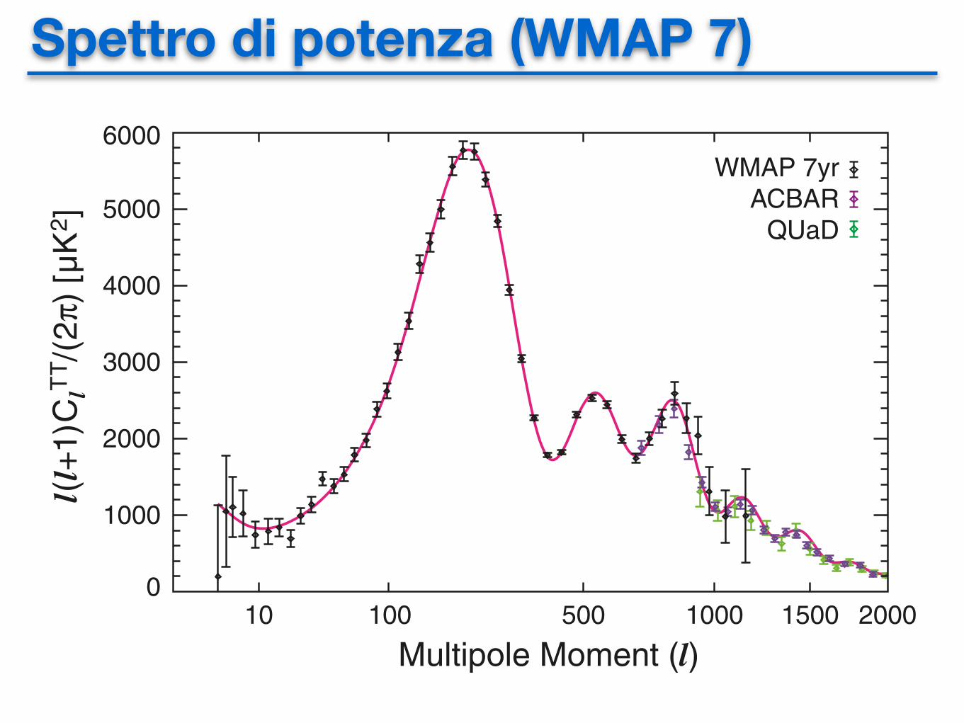
Spettro di potenza (WMAP 7)14 Komatsu et al.

Fig. 7.— The WMAP 7-year temperature power spectrum (Larson et al. 2010), along with the temperature power spectra from theACBAR (Reichardt et al. 2009) and QUaD (Brown et al. 2009) experiments. We show the ACBAR and QUaD data only at l ! 690, wherethe errors in the WMAP power spectrum are dominated by noise. We do not use the power spectrum at l > 2000 because of a potentialcontribution from the SZ e!ect and point sources. The solid line shows the best-fitting 6-parameter flat "CDM model to the WMAP dataalone (see the 3rd column of Table 1 for the maximum likelihood parameters).

also found that the parameters of the minimal 6-parameter !CDM model derived from two compilationsof Kessler et al. (2009) are di"erent: one compilationuses the light curve fitter called SALT-II (Guy et al. 2007)while the other uses the light curve fitter calledMLCS2K2(Jha et al. 2007). For example, #! derived fromWMAP+BAO+SALT-II and WMAP+BAO+MLCS2K2are di"erent by nearly 2!, despite being derived from thesame data sets (but processed with two di"erent lightcurve fitters). If we allow the dark energy equation ofstate parameter, w, to vary, we find that w derived fromWMAP+BAO+SALT-II and WMAP+BAO+MLCS2K2are di"erent by ! 2.5!.At the moment it is not obvious how to estimate sys-

tematic errors and properly incorporate them in the like-lihood analysis, in order to reconcile di"erent methodsand data sets.In this paper, we shall use one compilation of

the supernova data called the “Constitution” samples(Hicken et al. 2009b). The reason for this choice overthe others, such as the compilation by Kessler et al.(2009) that includes the latest data from the SDSS-IIsupernova survey, is that the Constitution samples arean extension of the “Union” samples (Kowalski et al.2008) that we used for the 5-year analysis (see Sec-tion 2.3 of Komatsu et al. 2009a). More specifically,the Constitution samples are the Union samples plusthe latest samples of nearby Type Ia supernovae opti-cal photometry from the Center for Astrophysics (CfA)supernova group (CfA3 sample; Hicken et al. 2009a).

Therefore, the parameter constraints from a combina-tion of the WMAP 7-year data, the latest BAO datadescribed above (Percival et al. 2009), and the Consti-tution supernova data may be directly compared to the“WMAP+BAO+SN” parameters given in Table 1 and2 of Komatsu et al. (2009a). This is a useful compari-son, as it shows how much the limits on parameters haveimproved by adding two more years of data.However, given the scatter of results among di"erent

compilations of the supernova data, we have decided tochoose the “WMAP+BAO+H0” (see Section 3.2.2) asour best data combination to constrain the cosmologi-cal parameters, except for dark energy parameters. Fordark energy parameters, we compare the results fromWMAP+BAO+H0 and WMAP+BAO+SN in Section 5.Note that we always marginalize over the absolute mag-nitudes of Type Ia supernovae with a uniform prior.

3.2.5. Time-delay Distance

Can we measure angular diameter distances out tohigher redshifts? Measurements of gravitational lensingtime delays o"er a way to determine absolute distancescales (Refsdal 1964). When a foreground galaxy lenses abackground variable source (e.g., quasars) and producesmultiple images of the source, changes of the source lu-minosity due to variability appear on multiple images atdi"erent times.The time delay at a given image position ! for a given

source position ", t(!,"), depends on the angular diam-eter distances as (see, e.g., Schneider et al. 2006, for a

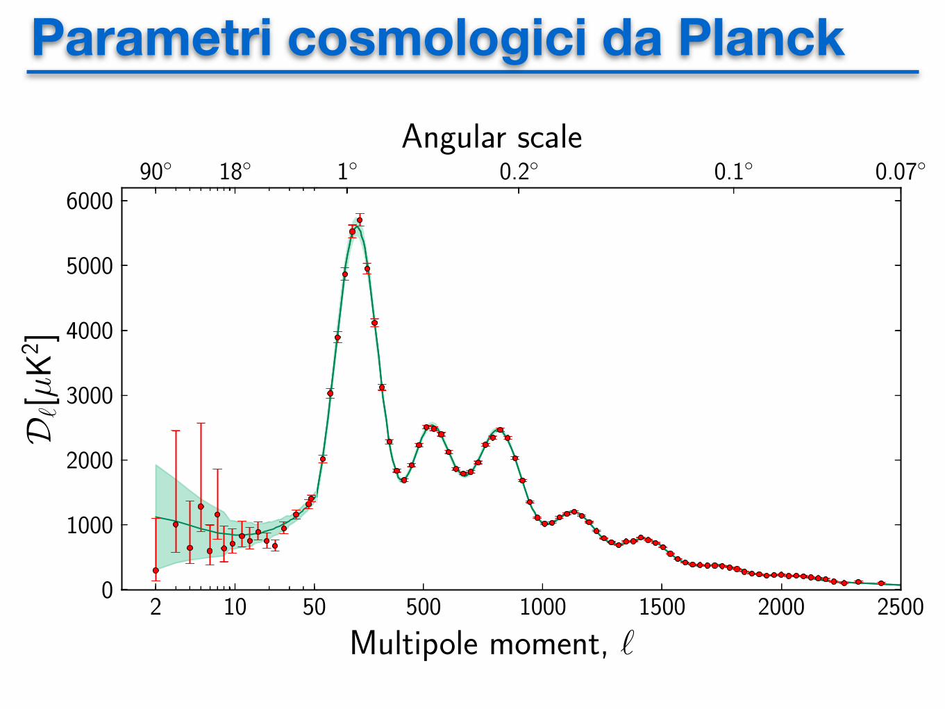
Parametri cosmologici da PlanckPlanck collaboration: CMB power spectra & likelihood

2 10 500

1000

2000

3000

4000

5000

6000

D�[µK

2 ]

90� 18�

500 1000 1500 2000 2500

Multipole moment, �

1� 0.2� 0.1� 0.07�Angular scale

Figure 37. The 2013 Planck CMB temperature angular power spectrum. The error bars include cosmic variance, whose magnitudeis indicated by the green shaded area around the best fit model. The low-` values are plotted at 2, 3, 4, 5, 6, 7, 8, 9.5, 11.5, 13.5, 16,19, 22.5, 27, 34.5, and 44.5.

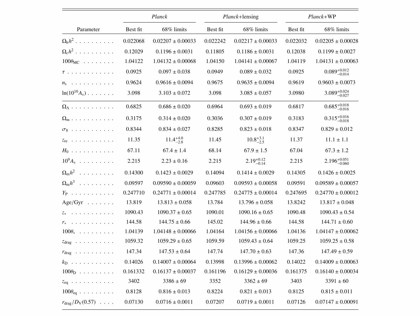
Table 8. Constraints on the basic six-parameter ⇤CDM model using Planck data. The top section contains constraints on the sixprimary parameters included directly in the estimation process, and the bottom section contains constraints on derived parameters.

Planck Planck+WP

Parameter Best fit 68% limits Best fit 68% limits

⌦bh2 . . . . . . . . . 0.022068 0.02207 ± 0.00033 0.022032 0.02205 ± 0.00028

⌦ch2 . . . . . . . . . 0.12029 0.1196 ± 0.0031 0.12038 0.1199 ± 0.0027100✓MC . . . . . . . 1.04122 1.04132 ± 0.00068 1.04119 1.04131 ± 0.00063

⌧ . . . . . . . . . . . . 0.0925 0.097 ± 0.038 0.0925 0.089+0.012�0.014

ns . . . . . . . . . . . 0.9624 0.9616 ± 0.0094 0.9619 0.9603 ± 0.0073

ln(1010As) . . . . . 3.098 3.103 ± 0.072 3.0980 3.089+0.024�0.027

⌦⇤ . . . . . . . . . . 0.6825 0.686 ± 0.020 0.6817 0.685+0.018�0.016

⌦m . . . . . . . . . . 0.3175 0.314 ± 0.020 0.3183 0.315+0.016�0.018

�8 . . . . . . . . . . . 0.8344 0.834 ± 0.027 0.8347 0.829 ± 0.012

zre . . . . . . . . . . . 11.35 11.4+4.0�2.8 11.37 11.1 ± 1.1

H0 . . . . . . . . . . 67.11 67.4 ± 1.4 67.04 67.3 ± 1.2

109As . . . . . . . . 2.215 2.23 ± 0.16 2.215 2.196+0.051�0.060

⌦mh2 . . . . . . . . . 0.14300 0.1423 ± 0.0029 0.14305 0.1426 ± 0.0025Age/Gyr . . . . . . 13.819 13.813 ± 0.058 13.8242 13.817 ± 0.048z⇤ . . . . . . . . . . . 1090.43 1090.37 ± 0.65 1090.48 1090.43 ± 0.54100✓⇤ . . . . . . . . 1.04139 1.04148 ± 0.00066 1.04136 1.04147 ± 0.00062zeq . . . . . . . . . . . 3402 3386 ± 69 3403 3391 ± 60

33

Planck Collaboration: Cosmological parameters

Planck Planck+lensing Planck+WP

Parameter Best fit 68% limits Best fit 68% limits Best fit 68% limits

⌦bh2 . . . . . . . . . . 0.022068 0.02207 ± 0.00033 0.022242 0.02217 ± 0.00033 0.022032 0.02205 ± 0.00028

⌦ch2 . . . . . . . . . . 0.12029 0.1196 ± 0.0031 0.11805 0.1186 ± 0.0031 0.12038 0.1199 ± 0.0027

100✓MC . . . . . . . . 1.04122 1.04132 ± 0.00068 1.04150 1.04141 ± 0.00067 1.04119 1.04131 ± 0.00063

⌧ . . . . . . . . . . . . 0.0925 0.097 ± 0.038 0.0949 0.089 ± 0.032 0.0925 0.089+0.012�0.014

ns . . . . . . . . . . . 0.9624 0.9616 ± 0.0094 0.9675 0.9635 ± 0.0094 0.9619 0.9603 ± 0.0073

ln(1010As) . . . . . . . 3.098 3.103 ± 0.072 3.098 3.085 ± 0.057 3.0980 3.089+0.024�0.027

⌦⇤ . . . . . . . . . . . 0.6825 0.686 ± 0.020 0.6964 0.693 ± 0.019 0.6817 0.685+0.018�0.016

⌦m . . . . . . . . . . . 0.3175 0.314 ± 0.020 0.3036 0.307 ± 0.019 0.3183 0.315+0.016�0.018

�8 . . . . . . . . . . . 0.8344 0.834 ± 0.027 0.8285 0.823 ± 0.018 0.8347 0.829 ± 0.012

zre . . . . . . . . . . . 11.35 11.4+4.0�2.8 11.45 10.8+3.1

�2.5 11.37 11.1 ± 1.1

H0 . . . . . . . . . . . 67.11 67.4 ± 1.4 68.14 67.9 ± 1.5 67.04 67.3 ± 1.2

109As . . . . . . . . . 2.215 2.23 ± 0.16 2.215 2.19+0.12�0.14 2.215 2.196+0.051

�0.060

⌦mh2 . . . . . . . . . 0.14300 0.1423 ± 0.0029 0.14094 0.1414 ± 0.0029 0.14305 0.1426 ± 0.0025

⌦mh3 . . . . . . . . . 0.09597 0.09590 ± 0.00059 0.09603 0.09593 ± 0.00058 0.09591 0.09589 ± 0.00057

YP . . . . . . . . . . . 0.247710 0.24771 ± 0.00014 0.247785 0.24775 ± 0.00014 0.247695 0.24770 ± 0.00012

Age/Gyr . . . . . . . 13.819 13.813 ± 0.058 13.784 13.796 ± 0.058 13.8242 13.817 ± 0.048

z⇤ . . . . . . . . . . . 1090.43 1090.37 ± 0.65 1090.01 1090.16 ± 0.65 1090.48 1090.43 ± 0.54

r⇤ . . . . . . . . . . . 144.58 144.75 ± 0.66 145.02 144.96 ± 0.66 144.58 144.71 ± 0.60

100✓⇤ . . . . . . . . . 1.04139 1.04148 ± 0.00066 1.04164 1.04156 ± 0.00066 1.04136 1.04147 ± 0.00062

zdrag . . . . . . . . . . 1059.32 1059.29 ± 0.65 1059.59 1059.43 ± 0.64 1059.25 1059.25 ± 0.58

rdrag . . . . . . . . . . 147.34 147.53 ± 0.64 147.74 147.70 ± 0.63 147.36 147.49 ± 0.59

kD . . . . . . . . . . . 0.14026 0.14007 ± 0.00064 0.13998 0.13996 ± 0.00062 0.14022 0.14009 ± 0.00063

100✓D . . . . . . . . . 0.161332 0.16137 ± 0.00037 0.161196 0.16129 ± 0.00036 0.161375 0.16140 ± 0.00034

zeq . . . . . . . . . . . 3402 3386 ± 69 3352 3362 ± 69 3403 3391 ± 60

100✓eq . . . . . . . . . 0.8128 0.816 ± 0.013 0.8224 0.821 ± 0.013 0.8125 0.815 ± 0.011

rdrag/DV(0.57) . . . . 0.07130 0.0716 ± 0.0011 0.07207 0.0719 ± 0.0011 0.07126 0.07147 ± 0.00091

Table 2. Cosmological parameter values for the six-parameter base ⇤CDM model. Columns 2 and 3 give results for the Plancktemperature power spectrum data alone. Columns 4 and 5 combine the Planck temperature data with Planck lensing, and columns6 and 7 include WMAP polarization at low multipoles. We give best fit parameters as well as 68% confidence limits for constrainedparameters. The first six parameters have flat priors. The remainder are derived parameters as discussed in Sect. 2. Beam, calibrationparameters, and foreground parameters (see Sect. 4) are not listed for brevity. Constraints on foreground parameters for Planck+WPare given later in Table 5.

3.2. Hubble parameter and dark energy density

The Hubble constant, H0, and matter density parameter, ⌦m,are only tightly constrained in the combination ⌦mh3 discussedabove, but the extent of the degeneracy is limited by the e↵ectof ⌦mh2 on the relative heights of the acoustic peaks. The pro-jection of the constraint ellipse shown in Fig. 3 onto the axestherefore yields useful marginalized constraints on H0 and ⌦m(or equivalently ⌦⇤) separately. We find the 2% constraint onH0:

H0 = (67.4 ± 1.4) km s�1 Mpc�1 (68%; Planck). (13)

The corresponding constraint on the dark energy density param-eter is

⌦⇤ = 0.686 ± 0.020 (68%; Planck), (14)

and for the physical matter density we find

⌦mh2 = 0.1423 ± 0.0029 (68%; Planck). (15)

Note that these indirect constraints are highly model depen-dent. The data only measure accurately the acoustic scale, and

the relation to underlying expansion parameters (e.g., via theangular-diameter distance) depends on the assumed cosmology,including the shape of the primordial fluctuation spectrum. Evensmall changes in model assumptions can change H0 noticeably;for example, if we neglect the 0.06 eV neutrino mass expectedin the minimal hierarchy, and instead take

Pm⌫ = 0, the Hubble

parameter constraint shifts to

H0 = (68.0 ± 1.4) km s�1 Mpc�1 (68%; Planck,P

m⌫ = 0). (16)

3.3. Matter densities

Planck can measure the matter densities in baryons and darkmatter from the relative heights of the acoustic peaks. However,as discussed above, there is a partial degeneracy with the spec-tral index and other parameters that limits the precision of thedetermination. With Planck there are now enough well measuredpeaks that the extent of the degeneracy is limited, giving ⌦bh2 toan accuracy of 1.5% without any additional data:

⌦bh2 = 0.02207 ± 0.00033 (68%; Planck). (17)

11

CAMBProgramma che risolve eq. Einstein, eq. Boltzmann, eq. fluide per determinare lo spettro delle fluttuazioni di temperatura (e della polarizzazione).

Disponibile liberamente: http://camb.info/ (sorgente F90)

Interfaccia web:http://lambda.gsfc.nasa.gov/toolbox/tb_camb_form.cfm

Altri toolshttp://lambda.gsfc.nasa.gov/toolbox/