FINITE STRAIN AND INFINITESIMAL STRAIN · mathematical treatment than finite strain (e.g.,...

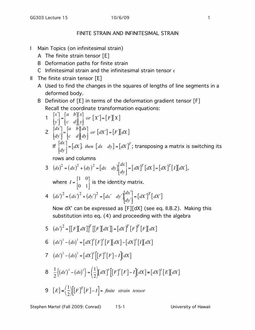
GG303 Lecture 15 10/6/09 1

Stephen Martel (Fall 2009: Conrad) 15-1 University of Hawaii

FINITE STRAIN AND INFINITESIMAL STRAIN I Main Topics (on infinitesimal strain)

A The finite strain tensor [E] B Deformation paths for finite strain C Infinitesimal strain and the infinitesimal strain tensor ε

II The finite strain tensor [E] A Used to find the changes in the squares of lengths of line segments in a

deformed body. B Definition of [E] in terms of the deformation gradient tensor [F]

Recall the coordinate transformation equations: 1

!

" x

" y

#

$ % &

' ( =

a b

c d

#

$ % &

' ( x

y

#

$ % &

' ( or " X [ ] = F[ ] X[ ]

2

!

d " x

d " y

#

$ % &

' ( =

a b

c d

#

$ % &

' ( dx

dy

#

$ % &

' ( or d " X [ ] = F[ ] dX[ ]

If

!

dx

dy

"

# $ %

& ' = dX[ ], then dx dy[ ] = dX[ ]

T ; transposing a matrix is switching its

rows and columns 3

!

ds( )2

= dx( )2

+ dy( )2

= dx dy[ ]dx

dy

"

# $ %

& ' = dX[ ]

TdX[ ] = dX[ ]

TI[ ] dX[ ],

where

!

I =1 0

0 1

"

# $ %

& ' is the identity matrix.

4

!

d " s ( )2

= d " x ( )2

+ d " y ( )2

= d " x d " y [ ]d " x

d " y

#

$ % &

' ( = d " X [ ]

Td " X [ ]

Now dX’ can be expressed as [F][dX] (see eq. II.B.2). Making this substitution into eq. (4) and proceeding with the algebra

5

!

d " s ( )2

= F[ ] dX[ ][ ]T

F[ ] dX[ ][ ] = dX[ ]T

F[ ]T

F[ ] dX[ ]

6

!

d " s ( )2

# ds( )2

= dX[ ]T

F[ ]T

F[ ] dX[ ] # dX[ ]T

I[ ] dX[ ]

7

!

d " s ( )2

# ds( )2

= dX[ ]T

F[ ]T

F[ ] # I[ ] dX[ ]

8

!

1

2d " s ( )

2

# ds( )2{ } =

1

2

$

% & '

( ) dX[ ]

T

F[ ]T

F[ ] # I[ ] dX[ ] * dX[ ]T

E[ ] dX[ ]

9

!

E[ ] "1

2

# $ % & F[ ]

TF[ ] ' I[ ] = finite strain tensor

GG303 Lecture 15 10/6/09 2


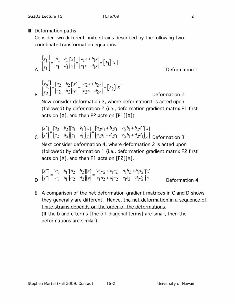
III Deformation paths Consider two different finite strains described by the following two coordinate transformation equations:

A

!

x1"

y1"

#

$ %

&

' ( =

a1 b1

c1 d1

#

$ %

&

' (

x

y

#

$ % &

' ( =a1x + b1y

c1x + d1y

#

$ %

&

' ( = F1[ ] X[ ]

Deformation 1

B

!

x2"

y2"

#

$ %

&

' ( =

a2 b2

c2 d2

#

$ %

&

' (

x

y

#

$ % &

' ( =a2x + b2y

c2x + d2y

#

$ %

&

' ( = F2[ ] X[ ]

Deformation 2 Now consider deformation 3, where deformation1 is acted upon (followed) by deformation 2 (i.e., deformation gradient matrix F1 first acts on [X], and then F2 acts on [F1][X])

C

!

" " x

" " y

#

$ % &

' ( =

a2 b2

c2 d2

#

$ %

&

' (

a1 b1

c1 d1

#

$ %

&

' (

x

y

#

$ % &

' ( =

a2a1 + b2c1 a2b1 + b2d1

c2a1 + d2c1 c2b1 + d2d1

#

$ %

&

' (

x

y

#

$ % &

' ( Deformation 3 Next consider deformation 4, where deformation 2 is acted upon (followed) by deformation 1 (i.e., deformation gradient matrix F2 first acts on [X], and then F1 acts on [F2][X].

D

!

" " " x

" " " y

#

$ % &

' ( =

a1 b1

c1 d1

#

$ %

&

' (

a2 b2

c2 d2

#

$ %

&

' (

x

y

#

$ % &

' ( =

a1a2 + b1c2 a1b2 + b1d2

c1a2 + d1c2 c1b2 + d1d2

#

$ %

&

' (

x

y

#

$ % &

' ( Deformation 4

E A comparison of the net deformation gradient matrices in C and D shows

they generally are different. Hence, the net deformation in a sequence of finite strains depends on the order of the deformations.

(If the b and c terms [the off-diagonal terms] are small, then the deformations are similar)

GG303 Lecture 15 10/6/09 3


GG303 Lecture 15 10/6/09 4


IV Infinitesimal strain and the infinitesimal strain tensor [ε]

A What is infinitesimal strain?

Deformation where the displacement derivatives are small relative to one (i.e., the terms in the corresponding displacement gradient matrix

!

Ju[ ] are

very small), so that the products of the derivatives are very small and can

be ignored.

B Why consider infinitesimal strain if it is an approximation?

1 Many important geologic deformations are small (and largely elastic)

over short time frames (e.g., fracture earthquake deformation, volcano

deformation).

2 The terms of the infinitesimal strain tensor [ε] have clear geometric

meaning (clearer than those for finite strain) 3 Infinitesimal strain is much more amenable to sophisticated

mathematical treatment than finite strain (e.g., elasticity theory). 4 The net deformation for infinitesimal strain is independent of the

deformation sequence. 5 Example

!

F5 =1.02 0.01

0 1.01

"

# $ %

& '

!

F6 =1.01 0

0 1.02

"

# $ %

& '

!

Ju5 =

0.02 0.01

0 0.01

"

# $ %

& '

!

Ju6 =

0.01 0

0 0.02

"

# $ %

& '

Deformation 5 followed by deformation 6 gives deformation 7:

!

" x

" y

#

$ % &

' ( =1.01 0.00

0.00 1.02

#

$ % &

' ( 1.02 0.01

0.00 1.01

#

$ % &

' ( x

y

#

$ % &

' ( =1.0302 0.0100

0.0000 1.0302

#

$ % &

' ( x

y

#

$ % &

' (

Deformation 6 followed by deformation 5 gives deformation “7a”:

!

" x

" y

#

$ % &

' ( =1.02 0.01

0.00 1.01

#

$ % &

' ( 1.01 0.00

0.00 1.02

#

$ % &

' ( x

y

#

$ % &

' ( =1.0302 0.0101

0.0000 1.0302

#

$ % &

' ( x

y

#

$ % &

' (

The net deformation is essentially the same in the two cases.

GG303 Lecture 15 10/6/09 5


C The infinitesimal strain tensor (Taylor series derivation)

Consider the displacement of two neighboring points, where the distance

from point 0 to point 1 initially is given by dx and dy. Point 0 is displaced

by an amount

!

u0, and we wish to find

!

u1. We use a truncated Taylor

series; it is linear in dx and dy (dx and dy are only raised to the first

power).

1

!

ux1 = u

x0 +

"ux

"xdx +

"ux

"ydy + ...

2

!

uy1 = u

y0 +

"uy

"xdx +

"uy

"ydy + ...

These can be rearranged into a matrix format:

3

!

ux1

uy1

"

#

$ $

%

&

' '

=ux0

uy0

"

#

$ $

%

&

' '

+

(ux

(x

(ux

(y(uy

(x

(uy

(y

"

#

$

$

$

%

&

'

'

'

dx

dy

"

# $ %

& ' = U

0" #

% &

+ Ju[ ] dX[ ]

Now split

!

Ju[ ] into two matrices: the symmetric infinitesimal strain matrix

[ε], and the anti-symmetric rotation matrix [ω] by using

!

Ju[ ]T

,

!

Ju[ ] =

e f

g h

"

# $ %

& ' ,

!

Ju[ ]T

=e g

f h

"

# $ %

& ' ,

!

Ju

+ JuT[ ] =

e + e f + g

g + f h + h

"

# $ %

& ' ,

!

Ju" J

uT[ ] =

0 f " g

g " f 0

#

$ % &

' (

4

!

Ju[ ] =

1

2Ju

+ Ju[ ] +

1

2Ju

T

" Ju

T[ ] =1

2Ju

+ Ju

T[ ] +1

2Ju" J

u

T[ ] = #[ ] + $[ ]

Now the displacement expression can be expanded using [ε] and [ω]

5

!

"[ ] =1

2

#ux

#x+#ux

#x

$

% &

'

( )

#ux

#y+#uy

#x

$

% &

'

( )

#uy

#x+#ux

#y

$

% &

'

( )

#uy

#y+

#uy

#y

$

% &

'

( )

*

+

,

,

,

,

-

.

/

/

/

/

, 0[ ] =1

2

0 1#ux

#y1#uy

#x

$

% &

'

( )

1#uy

#x1#ux

#y

$

% &

'

( ) 0

*

+

,

,

,

,

-

.

/

/

/

/

Equations (3) and (5) show that the deformation can be decomposed into

a translation, a strain, and a rotation.

D Geometric interpretation of the infinitesimal strain components

GG303 Lecture 15 10/6/09 6


GG303 Lecture 15 10/6/09 7


GG303 Lecture 15 10/6/09 8


E Relationship between [ε] and [E]

From eq. II.B.9, [E] is defined in terms of deformation gradients:

1

!

E[ ] "1

2

# $ % & F[ ]

TF[ ] ' I[ ] = finite strain tensor

The tensor [E] also can be solved for in terms of displacement gradients because

!

F = Ju

+ I .

2

!

E[ ] =1

2

" # $ % Ju + I[ ]

TJu + I[ ] & I[ ]

3

!

E[ ] =1

2

" # $ %

&uxdx

&uxdy

&uydx

&uydy

'

(

)

) )

*

+

,

, ,

+1 0

0 1

'

( ) *

+ ,

'

(

)

) )

*

+

,

, ,

T

&uxdx

&uxdy

&uydx

&uydy

'

(

)

) )

*

+

,

, ,

+1 0

0 1

'

( ) *

+ ,

'

(

)

) )

*

+

,

, ,

-1 0

0 1

'

( ) *

+ ,

'

(

)

)

)

*

+

,

,

,

4

!

E[ ] =1

2

" # $ %

&uxdx

+1&uydx

&uxdy

&uy

dy+1

'

(

)

) )

*

+

,

, ,

&uxdx

+1&uxdy

&uydx

&uydy

+1

'

(

)

) )

*

+

,

, ,

-1 0

0 1

'

( ) *

+ ,

'

(

)

) )

*

+

,

, ,

5

!

E[ ] =1

2

" # $ %

&uxdx

+1" #

$ % &uxdx

+1" #

$ %

+&uy

dx

"

# ' $

% ( &uy

dx

"

# ' $

% ( )1

&uxdx

+1" #

$ % &uxdy

"

# ' $

% +&uy

dx

"

# ' $

% ( &uy

dy+1

"

# ' $

% (

&uxdy

"

# ' $

%

&uxdx

+1" #

$ %

+&uy

dy+1

"

# ' $

% ( &uy

dx

"

# ' $

% ( &ux

dy

"

# ' $

%

&uxdy

"

# ' $

% +&uy

dy+1

"

# ' $

% ( &uy

dy+1

"

# ' $

% ( )1

*

+

,

,

,

-

.

/

/

/

If the displacement gradients are small relative to 1, then the products of the displacements are very small relative to 1, and in infinitesimal strain theory they can be dropped, yielding [ε]:

6

!

"[ ] #1

2

$ % & '

(uxdx

$ %

& '

+(uxdx

$ %

& '

(uxdy

$

% ) &

' +(uydx

$

% ) &

'

(uxdy

$

% ) &

' +(uydx

$

% ) &

'

(uydy

$

% ) &

' +(uydy

$

% ) &

'

*

+

,

,

,

-

.

/

/

/

=1

2Ju[ ] + J

u[ ]T*

+ - .

This suggests that for multiple deformations, infinitesimal strains might be obtained by matrix addition (i.e., linear superposition) rather than by matrix multiplication; the former is simpler. Also see equation IV.C.5.

GG303 Lecture 15 10/6/09 9


7 Example of IV.B.5: [ε] from superposed vs. sequenced deformations

!

F5 =1.02 0.01

0 1.01

"

# $ %

& '

!

Ju5 =

0.02 0.01

0 0.01

"

# $ %

& '

!

F6 =1.01 0

0 1.02

"

# $ %

& '

!

Ju6 =

0.01 0

0 0.02

"

# $ %

& '

a Linear superposition, assuming infinitesimal strain (approx.) »F5 = [1.02 0.01;0.00 1.01] F5 = 1.0200 0.0100 0 1.0100

»F6 = [1.01 0.00;0.00 1.02] F6 = 1.0100 0 0 1.0200

!

E5 =1

2F5[ ]

T

F5[ ] " I[ ]

!

E6 =1

2F6[ ]

T

F6[ ] " I[ ]

»E5 = 0.5*(F5'*F5-eye(2))

E5 = 0.0202 0.0051 0.0051 0.0101

» E6 = 0.5*(F6'*F6-eye(2))

E6 = 0.0101 0 0 0.0202

!

"1

2Ju5[ ] + J

u5[ ]

T# $

% &

' (

) *

!

"1

2Ju6[ ] + J

u6[ ]

T# $

% &

' (

) *

»E7 = E5 + E6 Linear superposition of strains E7 = (Infinitesimal approximation) 0.0302 0.0051 0.0051 0.0303

b Sequenced deformation (exact)

!

E7[ ] " 1

2

# $ % & F7[ ]T

F7[ ] ' I

(

) * +

, -

»F7 = F6*F5 See eq. IV.B.5 F7 = 1.0302 0.0101 0 1.0302 »E7 = 0.5*(F7'*F7-eye(2)) Convert def. gradients to strain E7 = Good match with approximation 0.0307 0.0052 0.0052 0.0307

GG303 Lecture 15 10/6/09 10


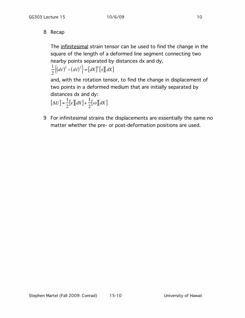
8 Recap

The infinitesimal strain tensor can be used to find the change in the square of the length of a deformed line segment connecting two nearby points separated by distances dx and dy,

!

1

2ds'( )2 " ds'( )2{ } = dX[ ]T #[ ] dX[ ]

and, with the rotation tensor, to find the change in displacement of two points in a deformed medium that are initially separated by distances dx and dy:

!

"U[ ] =1

2#[ ] dX[ ] +

1

2$[ ] dX[ ]

9 For infinitesimal strains the displacements are essentially the same no matter whether the pre- or post-deformation positions are used.

FINITE STRAIN AND INFINITESIMAL STRAIN · mathematical treatment than finite strain (e.g.,...

Documents

Transcript of FINITE STRAIN AND INFINITESIMAL STRAIN · mathematical treatment than finite strain (e.g.,...