Finite element method - TU Dortmundkuzmin/cfdintro/lecture6.pdf · Finite element method Origins:...
22
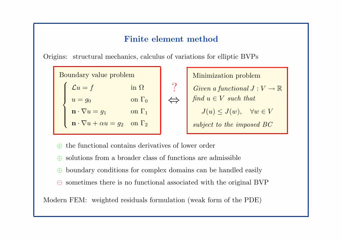
Finite element method Origins: structural mechanics, calculus of variations for elliptic BVPs Boundary value problem Lu = f in Ω u = g 0 on Γ 0 n ·∇u = g 1 on Γ 1 n ·∇u + αu = g 2 on Γ 2 ? ⇔ Minimization problem Given a functional J : V → R find u ∈ V such that J (u) ≤ J (w), ∀w ∈ V subject to the imposed BC ⊕ the functional contains derivatives of lower order ⊕ solutions from a broader class of functions are admissible ⊕ boundary conditions for complex domains can be handled easily ⊖ sometimes there is no functional associated with the original BVP Modern FEM: weighted residuals formulation (weak form of the PDE)
-
Upload
nguyenhanh -
Category
Documents
-
view
266 -
download
0
Transcript of Finite element method - TU Dortmundkuzmin/cfdintro/lecture6.pdf · Finite element method Origins:...
Finite element method
Origins: structural mechanics, calculus of variations for elliptic BVPs
Boundary value problem
Lu = f in Ω
u = g0 on Γ0
n · ∇u = g1 on Γ1
n · ∇u+ αu = g2 on Γ2
?
⇔
Minimization problem
Given a functional J : V → R
find u ∈ V such that
J(u) ≤ J(w), ∀w ∈ V
subject to the imposed BC
⊕ the functional contains derivatives of lower order
⊕ solutions from a broader class of functions are admissible
⊕ boundary conditions for complex domains can be handled easily
⊖ sometimes there is no functional associated with the original BVP
Modern FEM: weighted residuals formulation (weak form of the PDE)
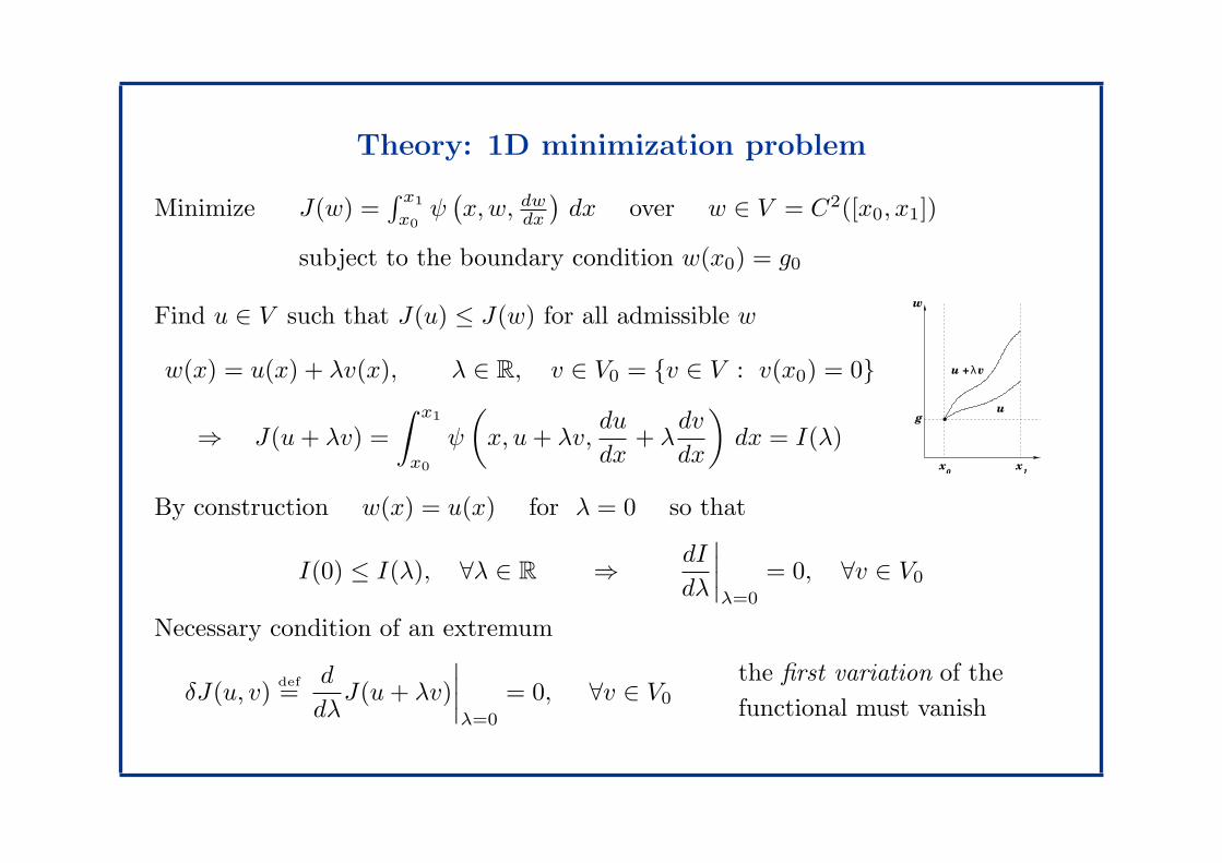
Theory: 1D minimization problem
Minimize J(w) =∫ x1
x0
ψ(x,w, dw
dx
)dx over w ∈ V = C2([x0, x1])
subject to the boundary condition w(x0) = g0
Find u ∈ V such that J(u) ≤ J(w) for all admissible w
w(x) = u(x) + λv(x), λ ∈ R, v ∈ V0 = v ∈ V : v(x0) = 0
⇒ J(u+ λv) =
∫ x1
x0
ψ
(
x, u+ λv,du
dx+ λ
dv
dx
)
dx = I(λ)
vλu +
x 0
x 1
w
gu
By construction w(x) = u(x) for λ = 0 so that
I(0) ≤ I(λ), ∀λ ∈ R ⇒dI
dλ
∣∣∣∣λ=0
= 0, ∀v ∈ V0
Necessary condition of an extremum
δJ(u, v)def
=d
dλJ(u+ λv)
∣∣∣∣λ=0
= 0, ∀v ∈ V0
the first variation of the
functional must vanish
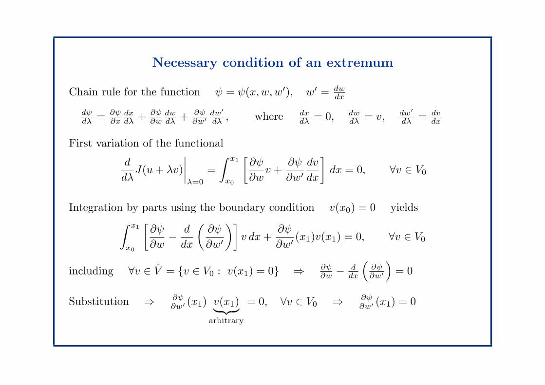
Necessary condition of an extremum
Chain rule for the function ψ = ψ(x,w,w′), w′ = dwdx
dψdλ
= ∂ψ∂x
dxdλ
+ ∂ψ∂w
dwdλ
+ ∂ψ∂w′
dw′
dλ, where dx
dλ= 0, dw
dλ= v, dw′
dλ= dv
dx
First variation of the functional
d
dλJ(u+ λv)
∣∣∣∣λ=0
=
∫ x1
x0
[∂ψ
∂wv +
∂ψ
∂w′
dv
dx
]
dx = 0, ∀v ∈ V0
Integration by parts using the boundary condition v(x0) = 0 yields
∫ x1
x0
[∂ψ
∂w−
d
dx
(∂ψ
∂w′
)]
v dx+∂ψ
∂w′(x1)v(x1) = 0, ∀v ∈ V0
including ∀v ∈ V = v ∈ V0 : v(x1) = 0 ⇒ ∂ψ∂w
− ddx
(∂ψ∂w′
)
= 0
Substitution ⇒ ∂ψ∂w′
(x1) v(x1)︸ ︷︷ ︸
arbitrary
= 0, ∀v ∈ V0 ⇒ ∂ψ∂w′
(x1) = 0
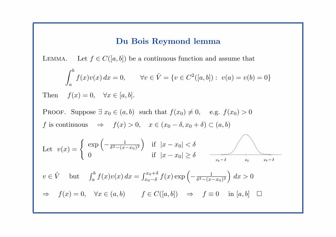
Du Bois Reymond lemma
Lemma. Let f ∈ C([a, b]) be a continuous function and assume that
∫ b
a
f(x)v(x) dx = 0, ∀v ∈ V = v ∈ C2([a, b]) : v(a) = v(b) = 0
Then f(x) = 0, ∀x ∈ [a, b].
Proof. Suppose ∃ x0 ∈ (a, b) such that f(x0) 6= 0, e.g. f(x0) > 0
f is continuous ⇒ f(x) > 0, x ∈ (x0 − δ, x0 + δ) ⊂ (a, b)
Let v(x) =
exp(
− 1δ2−(x−x0)2
)
if |x− x0| < δ
0 if |x− x0| ≥ δ x0x0 Æ x0 + Æ
v ∈ V but∫ b
af(x)v(x) dx =
∫ x0+δ
x0−δf(x) exp
(
− 1δ2−(x−x0)2
)
dx > 0
⇒ f(x) = 0, ∀x ∈ (a, b) f ∈ C([a, b]) ⇒ f ≡ 0 in [a, b]
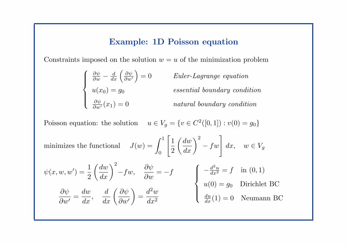
Example: 1D Poisson equation
Constraints imposed on the solution w = u of the minimization problem
∂ψ∂w
− ddx
(∂ψ∂w′
)
= 0 Euler-Lagrange equation
u(x0) = g0 essential boundary condition
∂ψ∂w′
(x1) = 0 natural boundary condition
Poisson equation: the solution u ∈ Vg = v ∈ C2([0, 1]) : v(0) = g0
minimizes the functional J(w) =
∫ 1
0
[
1
2
(dw
dx
)2
− fw
]
dx, w ∈ Vg
ψ(x,w,w′) =1
2
(dw
dx
)2
−fw,∂ψ
∂w= −f
∂ψ
∂w′=dw
dx,
d
dx
(∂ψ
∂w′
)
=d2w
dx2
−d2udx2 = f in (0, 1)
u(0) = g0 Dirichlet BC
dudx
(1) = 0 Neumann BC
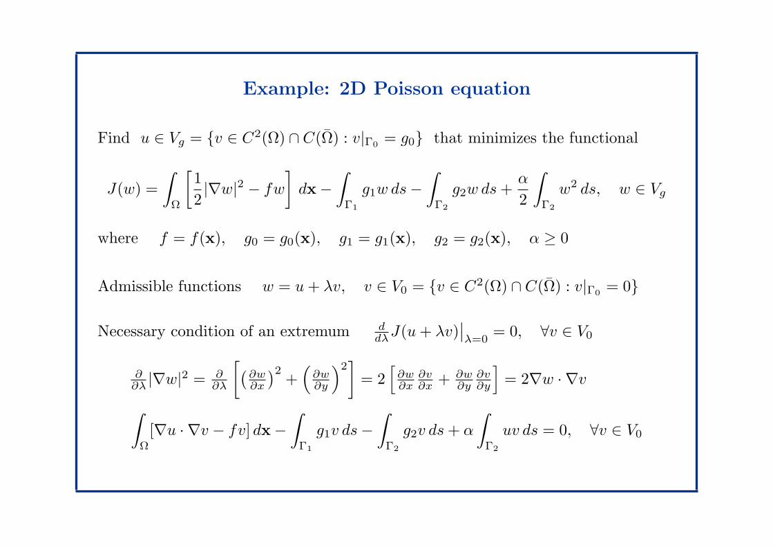
Example: 2D Poisson equation
Find u ∈ Vg = v ∈ C2(Ω) ∩ C(Ω) : v|Γ0= g0 that minimizes the functional
J(w) =
∫
Ω
[1
2|∇w|2 − fw
]
dx −
∫
Γ1
g1w ds−
∫
Γ2
g2w ds+α
2
∫
Γ2
w2 ds, w ∈ Vg
where f = f(x), g0 = g0(x), g1 = g1(x), g2 = g2(x), α ≥ 0
Admissible functions w = u+ λv, v ∈ V0 = v ∈ C2(Ω) ∩ C(Ω) : v|Γ0= 0
Necessary condition of an extremum ddλJ(u+ λv)
∣∣λ=0
= 0, ∀v ∈ V0
∂∂λ
|∇w|2 = ∂∂λ
[(∂w∂x
)2+
(∂w∂y
)2]
= 2[∂w∂x
∂v∂x
+ ∂w∂y
∂v∂y
]
= 2∇w · ∇v
∫
Ω
[∇u · ∇v − fv] dx −
∫
Γ1
g1v ds−
∫
Γ2
g2v ds+ α
∫
Γ2
uv ds = 0, ∀v ∈ V0
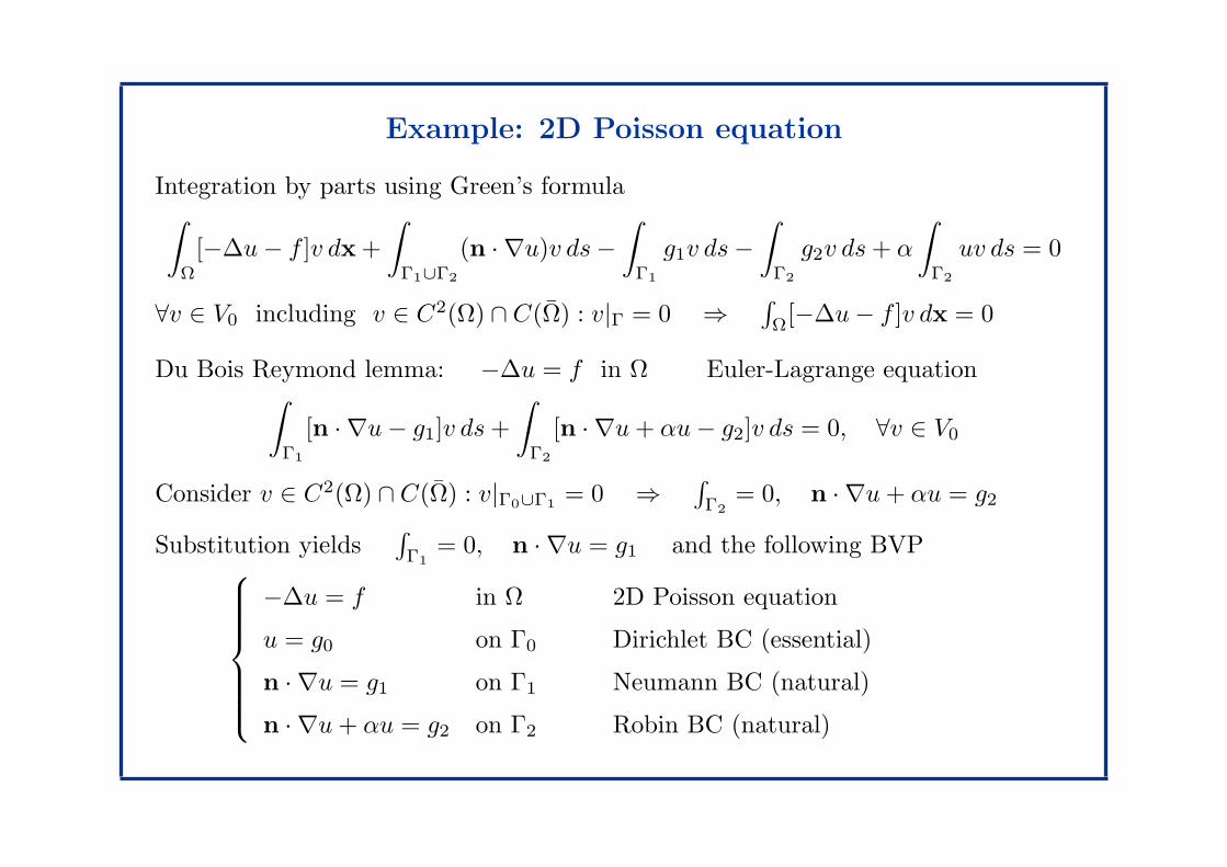
Example: 2D Poisson equation
Integration by parts using Green’s formula∫
Ω
[−∆u− f ]v dx +
∫
Γ1∪Γ2
(n · ∇u)v ds−
∫
Γ1
g1v ds−
∫
Γ2
g2v ds+ α
∫
Γ2
uv ds = 0
∀v ∈ V0 including v ∈ C2(Ω) ∩ C(Ω) : v|Γ = 0 ⇒∫
Ω[−∆u− f ]v dx = 0
Du Bois Reymond lemma: −∆u = f in Ω Euler-Lagrange equation∫
Γ1
[n · ∇u− g1]v ds+
∫
Γ2
[n · ∇u+ αu− g2]v ds = 0, ∀v ∈ V0
Consider v ∈ C2(Ω) ∩ C(Ω) : v|Γ0∪Γ1= 0 ⇒
∫
Γ2
= 0, n · ∇u+ αu = g2
Substitution yields∫
Γ1
= 0, n · ∇u = g1 and the following BVP
−∆u = f in Ω 2D Poisson equation
u = g0 on Γ0 Dirichlet BC (essential)
n · ∇u = g1 on Γ1 Neumann BC (natural)
n · ∇u+ αu = g2 on Γ2 Robin BC (natural)
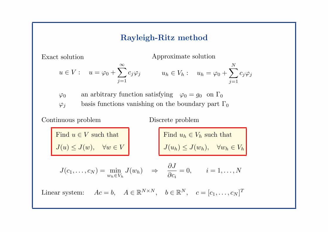
Rayleigh-Ritz method
Exact solution
u ∈ V : u = ϕ0 +
∞∑
j=1
cjϕj
Approximate solution
uh ∈ Vh : uh = ϕ0 +N∑
j=1
cjϕj
ϕ0 an arbitrary function satisfying ϕ0 = g0 on Γ0
ϕj basis functions vanishing on the boundary part Γ0
Continuous problem
Find u ∈ V such that
J(u) ≤ J(w), ∀w ∈ V
Discrete problem
Find uh ∈ Vh such that
J(uh) ≤ J(wh), ∀wh ∈ Vh
J(c1, . . . , cN ) = minwh∈Vh
J(wh) ⇒∂J
∂ci= 0, i = 1, . . . , N
Linear system: Ac = b, A ∈ RN×N , b ∈ R
N , c = [c1, . . . , cN ]T
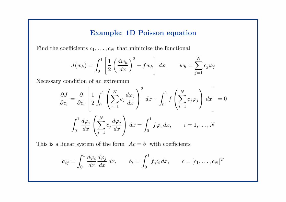
Example: 1D Poisson equation
Find the coefficients c1, . . . , cN that minimize the functional
J(wh) =
∫ 1
0
[
1
2
(dwhdx
)2
− fwh
]
dx, wh =
N∑
j=1
cjϕj
Necessary condition of an extremum
∂J
∂ci=
∂
∂ci
1
2
∫ 1
0
N∑
j=1
cjdϕjdx
2
dx−
∫ 1
0
f
N∑
j=1
cjϕj
dx
= 0
∫ 1
0
dϕidx
N∑
j=1
cjdϕjdx
dx =
∫ 1
0
fϕi dx, i = 1, . . . , N
This is a linear system of the form Ac = b with coefficients
aij =
∫ 1
0
dϕidx
dϕjdx
dx, bi =
∫ 1
0
fϕi dx, c = [c1, . . . , cN ]T
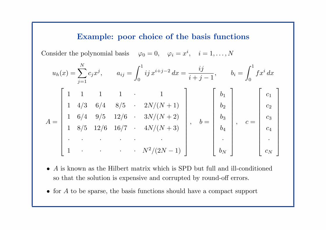
Example: poor choice of the basis functions
Consider the polynomial basis ϕ0 = 0, ϕi = xi, i = 1, . . . , N
uh(x) =
N∑
j=1
cjxj , aij =
∫ 1
0
ij xi+j−2 dx =ij
i+ j − 1, bi =
∫ 1
0
fxi dx
A =
1 1 1 1 · 1
1 4/3 6/4 8/5 · 2N/(N + 1)
1 6/4 9/5 12/6 · 3N/(N + 2)
1 8/5 12/6 16/7 · 4N/(N + 3)
· · · · · ·
1 · · · · N2/(2N − 1)
, b =
b1
b2
b3
b4
·
bN
, c =
c1
c2
c3
c4
·
cN
• A is known as the Hilbert matrix which is SPD but full and ill-conditioned
so that the solution is expensive and corrupted by round-off errors.
• for A to be sparse, the basis functions should have a compact support
Fundamentals of the FEM
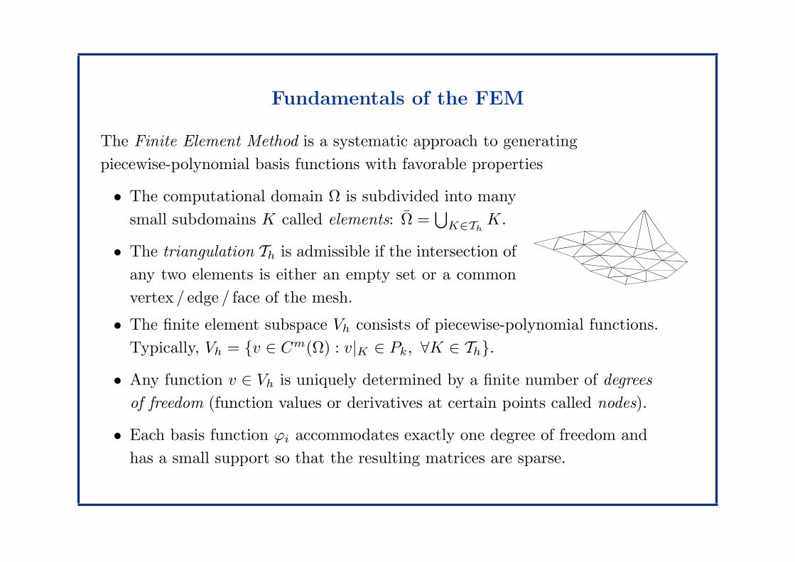
The Finite Element Method is a systematic approach to generating
piecewise-polynomial basis functions with favorable properties
• The computational domain Ω is subdivided into many
small subdomains K called elements: Ω =⋃
K∈ThK.
• The triangulation Th is admissible if the intersection of
any two elements is either an empty set or a common
vertex / edge / face of the mesh.Figure 4: Two nodal basis functions for the polygonal domain examplecomprising the right hand side as well as the entriesai;j = a(j; i) = Zri rj dx; i; j = 1; : : : N; (12)of the nite element system matrix A. This is where the advantage of the nodal basisfunction becomes apparent: the above integrals reduce to integrals over supp(i) in therst case and supp(i)\supp(j) in the second. The supports of two nodal basis functionsfor linear triangles consists of all those triangles of which the corresponding node is avertex. The supports of two basis functions in our example are shown in Figure 5.
Figure 5: Supports of 22 (left) and 27 (middle) and their common support (right)Thus, whenever basis functions with small support are used, all integrations need onlybe performed over a small number of elements. Rather than computing the integrals (11)and (12) successively, it is common practice in nite element software to traverse the gridelement by element and, for each element, to compute the partial sums of all integralsinvolving this element. These partial sums are then added to the appropriate componentsof A and f .The basis functions whose supports lie in a given element are termed the local basisfunctions belonging to this element. In our example using linear triangles, there are threelocal basis functions on each triangle K, say p; q and r, and we denote their restrictionto K by 'K1 = (p)jK; 'K2 = (q)jK and 'K3 = (r)jK:This introduces a local numbering of these basis functions on each element, i.e. on el-ement K, the (global) basis functions p; q and r are assigned the local numbers 1,2 and 3, respectively. We denote the mapping assigning local indices to p on elementK by i = GL(p;K) and the local to global mapping by p = LG(i; K). The quantities
• The finite element subspace Vh consists of piecewise-polynomial functions.
Typically, Vh = v ∈ Cm(Ω) : v|K ∈ Pk, ∀K ∈ Th.
• Any function v ∈ Vh is uniquely determined by a finite number of degrees
of freedom (function values or derivatives at certain points called nodes).
• Each basis function ϕi accommodates exactly one degree of freedom and
has a small support so that the resulting matrices are sparse.
Finite element approximation
The finite element is a triple (K,P,Σ), where
• K is a closed subset of Ω
• P is the polynomial space for the shape functions
• Σ is the set of local degrees of freedom
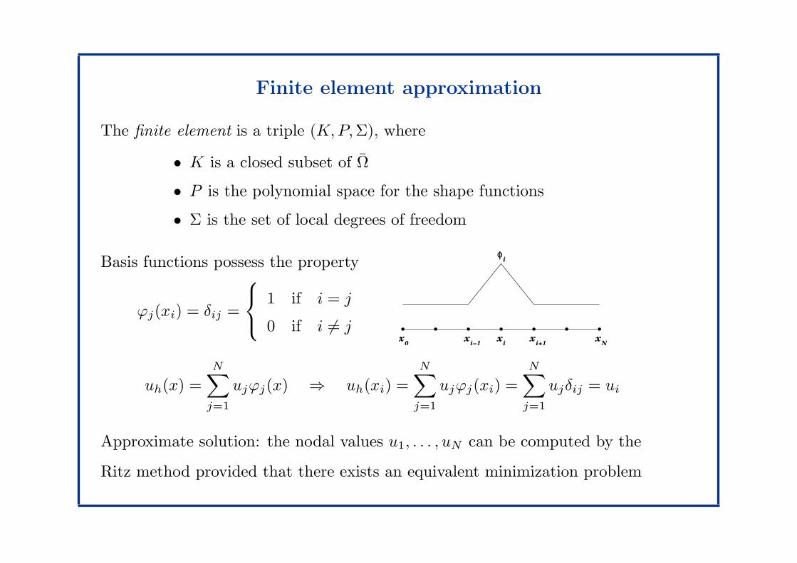
Basis functions possess the property
ϕj(xi) = δij =
1 if i = j
0 if i 6= j
ϕ i
ix x
i+1x
i−1x x
0 N
uh(x) =
N∑
j=1
ujϕj(x) ⇒ uh(xi) =
N∑
j=1
ujϕj(xi) =
N∑
j=1
ujδij = ui
Approximate solution: the nodal values u1, . . . , uN can be computed by the
Ritz method provided that there exists an equivalent minimization problem
Example: 1D Poisson equation
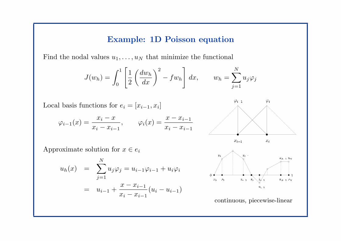
Find the nodal values u1, . . . , uN that minimize the functional
J(wh) =
∫ 1
0
[
1
2
(dwhdx
)2
− fwh
]
dx, wh =
N∑
j=1
ujϕj
Local basis functions for ei = [xi−1, xi]
ϕi−1(x) =xi − x
xi − xi−1, ϕi(x) =
x− xi−1
xi − xi−1
Approximate solution for x ∈ ei
uh(x) =
N∑
j=1
ujϕj = ui−1ϕi−1 + uiϕi
= ui−1 +x− xi−1
xi − xi−1(ui − ui−1)
xi1 xi'i1 'i
xNx1x0 xixi1 xN10 1
u1ui+1
uN1 uNui1xi+1
continuous, piecewise-linear
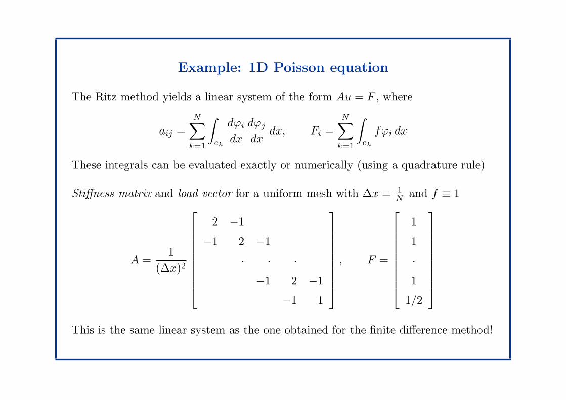
Example: 1D Poisson equation
The Ritz method yields a linear system of the form Au = F , where
aij =
N∑
k=1
∫
ek
dϕidx
dϕjdx
dx, Fi =
N∑
k=1
∫
ek
fϕi dx
These integrals can be evaluated exactly or numerically (using a quadrature rule)
Stiffness matrix and load vector for a uniform mesh with ∆x = 1N
and f ≡ 1
A =1
(∆x)2
2 −1
−1 2 −1
· · ·
−1 2 −1
−1 1
, F =
1
1
·
1
1/2
This is the same linear system as the one obtained for the finite difference method!
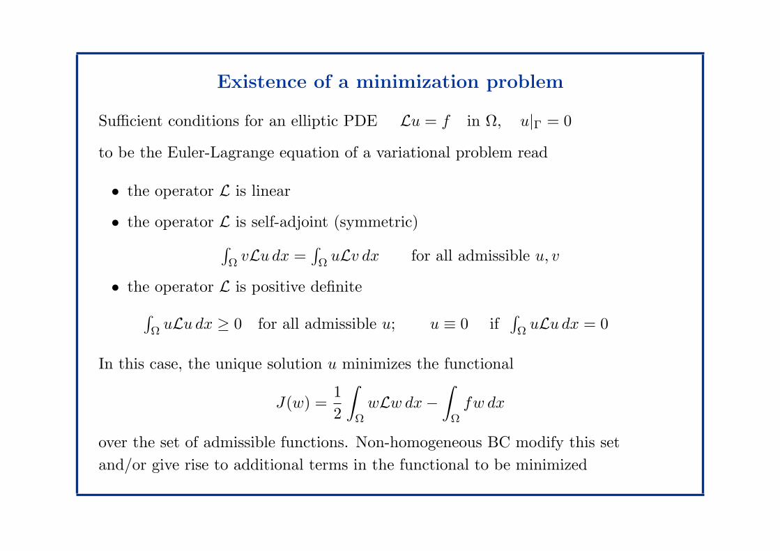
Existence of a minimization problem
Sufficient conditions for an elliptic PDE Lu = f in Ω, u|Γ = 0
to be the Euler-Lagrange equation of a variational problem read
• the operator L is linear
• the operator L is self-adjoint (symmetric)
∫
ΩvLu dx =
∫
ΩuLv dx for all admissible u, v
• the operator L is positive definite
∫
ΩuLu dx ≥ 0 for all admissible u; u ≡ 0 if
∫
ΩuLu dx = 0
In this case, the unique solution u minimizes the functional
J(w) =1
2
∫
Ω
wLw dx−
∫
Ω
fw dx
over the set of admissible functions. Non-homogeneous BC modify this set
and/or give rise to additional terms in the functional to be minimized
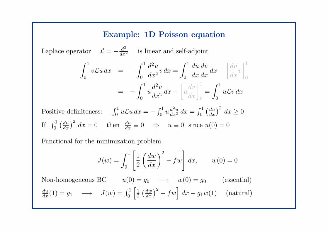
Example: 1D Poisson equation
Laplace operator L = − d2
dx2 is linear and self-adjoint
∫ 1
0
vLu dx = −
∫ 1
0
d2u
dx2v dx =
∫ 1
0
du
dx
dv
dxdx−
[du
dxv
]1
0
= −
∫ 1
0
ud2v
dx2dx+
[
udv
dx
]1
0
=
∫ 1
0
uLv dx
Positive-definiteness:∫ 1
0uLu dx = −
∫ 1
0ud
2udx2 dx =
∫ 1
0
(dudx
)2dx ≥ 0
If∫ 1
0
(dudx
)2dx = 0 then du
dx≡ 0 ⇒ u ≡ 0 since u(0) = 0
Functional for the minimization problem
J(w) =
∫ 1
0
[
1
2
(dw
dx
)2
− fw
]
dx, w(0) = 0
Non-homogeneous BC u(0) = g0 −→ w(0) = g0 (essential)
dudx
(1) = g1 −→ J(w) =∫ 1
0
[12
(dwdx
)2− fw
]
dx− g1w(1) (natural)
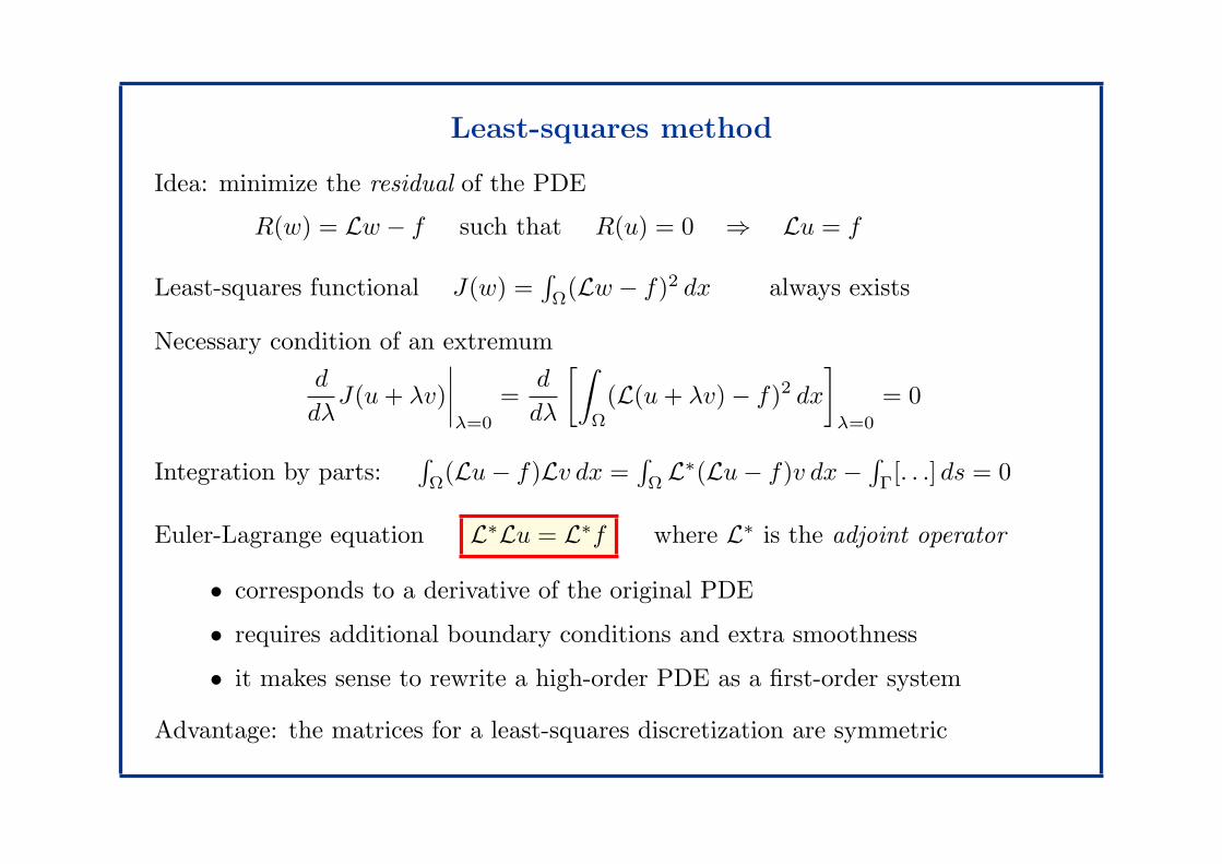
Least-squares method
Idea: minimize the residual of the PDE
R(w) = Lw − f such that R(u) = 0 ⇒ Lu = f
Least-squares functional J(w) =∫
Ω(Lw − f)2 dx always exists
Necessary condition of an extremum
d
dλJ(u+ λv)
∣∣∣∣λ=0
=d
dλ
[∫
Ω
(L(u+ λv) − f)2 dx
]
λ=0
= 0
Integration by parts:∫
Ω(Lu− f)Lv dx =
∫
ΩL∗(Lu− f)v dx−
∫
Γ[. . .] ds = 0
Euler-Lagrange equation L∗Lu = L∗f where L∗ is the adjoint operator
• corresponds to a derivative of the original PDE
• requires additional boundary conditions and extra smoothness
• it makes sense to rewrite a high-order PDE as a first-order system
Advantage: the matrices for a least-squares discretization are symmetric
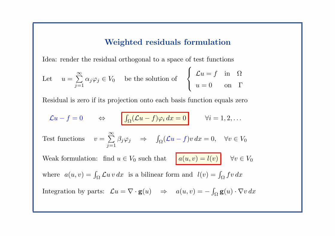
Weighted residuals formulation
Idea: render the residual orthogonal to a space of test functions
Let u =∞∑
j=1
αjϕj ∈ V0 be the solution of
Lu = f in Ω
u = 0 on Γ
Residual is zero if its projection onto each basis function equals zero
Lu− f = 0 ⇔∫
Ω(Lu− f)ϕi dx = 0 ∀i = 1, 2, . . .
Test functions v =∞∑
j=1
βjϕj ⇒∫
Ω(Lu− f)v dx = 0, ∀v ∈ V0
Weak formulation: find u ∈ V0 such that a(u, v) = l(v) ∀v ∈ V0
where a(u, v) =∫
ΩLu v dx is a bilinear form and l(v) =
∫
Ωfv dx
Integration by parts: Lu = ∇ · g(u) ⇒ a(u, v) = −∫
Ωg(u) · ∇v dx
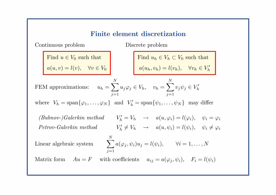
Finite element discretization
Continuous problem
Find u ∈ V0 such that
a(u, v) = l(v), ∀v ∈ V0
Discrete problem
Find uh ∈ Vh ⊂ V0 such that
a(uh, vh) = l(vh), ∀vh ∈ V ′h
FEM approximations: uh =
N∑
j=1
ujϕj ∈ Vh, vh =
N∑
j=1
vjψj ∈ V ′h
where Vh = spanϕ1, . . . , ϕN and V ′h = spanψ1, . . . , ψN may differ
(Bubnov-)Galerkin method V ′h = Vh → a(u, ϕi) = l(ϕi), ψi = ϕi
Petrov-Galerkin method V ′h 6= Vh → a(u, ψi) = l(ψi), ψi 6= ϕi
Linear algebraic system
N∑
j=1
a(ϕj , ψi)uj = l(ψi), ∀i = 1, . . . , N
Matrix form Au = F with coefficients aij = a(ϕj , ψi), Fi = l(ψi)
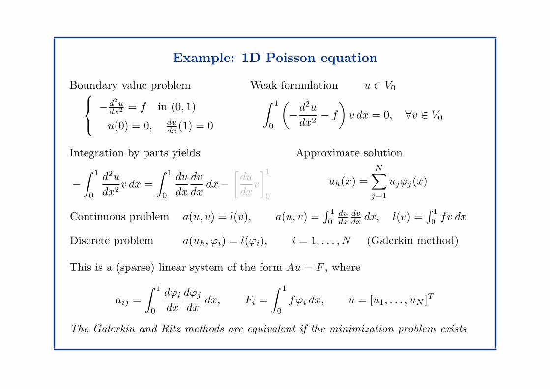
Example: 1D Poisson equation
Boundary value problem
−d2udx2 = f in (0, 1)
u(0) = 0, dudx
(1) = 0
Weak formulation u ∈ V0
∫ 1
0
(
−d2u
dx2− f
)
v dx = 0, ∀v ∈ V0
Integration by parts yields
−
∫ 1
0
d2u
dx2v dx =
∫ 1
0
du
dx
dv
dxdx−
[du
dxv
]1
0
Approximate solution
uh(x) =
N∑
j=1
ujϕj(x)
Continuous problem a(u, v) = l(v), a(u, v) =∫ 1
0dudx
dvdxdx, l(v) =
∫ 1
0fv dx
Discrete problem a(uh, ϕi) = l(ϕi), i = 1, . . . , N (Galerkin method)
This is a (sparse) linear system of the form Au = F , where
aij =
∫ 1
0
dϕidx
dϕjdx
dx, Fi =
∫ 1
0
fϕi dx, u = [u1, . . . , uN ]T
The Galerkin and Ritz methods are equivalent if the minimization problem exists
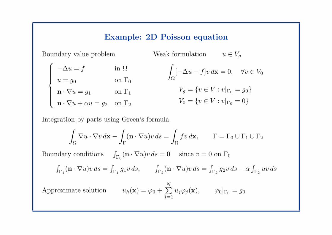
Example: 2D Poisson equation
Boundary value problem
−∆u = f in Ω
u = g0 on Γ0
n · ∇u = g1 on Γ1
n · ∇u+ αu = g2 on Γ2
Weak formulation u ∈ Vg∫
Ω
[−∆u− f ]v dx = 0, ∀v ∈ V0
Vg = v ∈ V : v|Γ0= g0
V0 = v ∈ V : v|Γ0= 0
Integration by parts using Green’s formula∫
Ω
∇u · ∇v dx −
∫
Γ
(n · ∇u)v ds =
∫
Ω
fv dx, Γ = Γ0 ∪ Γ1 ∪ Γ2
Boundary conditions∫
Γ0
(n · ∇u)v ds = 0 since v = 0 on Γ0
∫
Γ1
(n · ∇u)v ds =∫
Γ1
g1v ds,∫
Γ2
(n · ∇u)v ds =∫
Γ2
g2v ds− α∫
Γ2
uv ds
Approximate solution uh(x) = ϕ0 +N∑
j=1
ujϕj(x), ϕ0|Γ0= g0
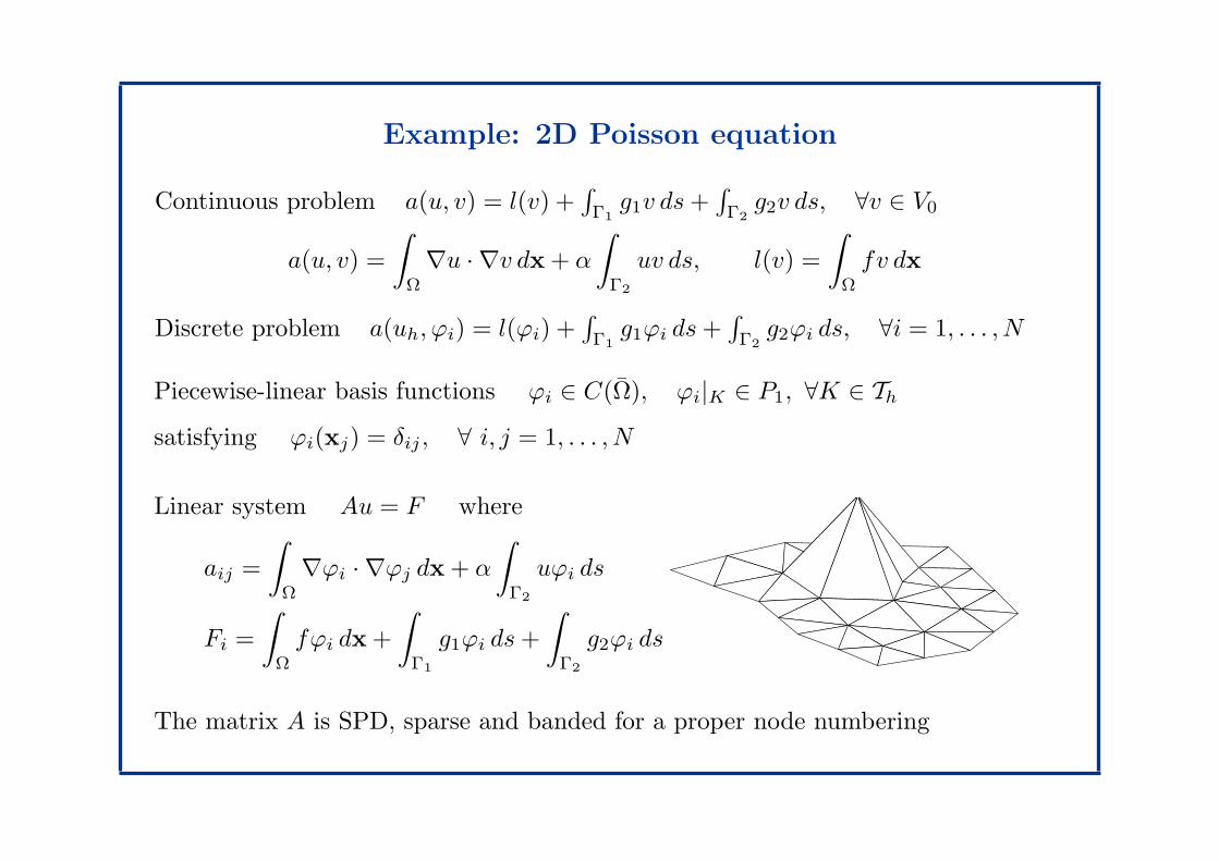
Example: 2D Poisson equation
Continuous problem a(u, v) = l(v) +∫
Γ1
g1v ds+∫
Γ2
g2v ds, ∀v ∈ V0
a(u, v) =
∫
Ω
∇u · ∇v dx + α
∫
Γ2
uv ds, l(v) =
∫
Ω
fv dx
Discrete problem a(uh, ϕi) = l(ϕi) +∫
Γ1
g1ϕi ds+∫
Γ2
g2ϕi ds, ∀i = 1, . . . , N
Piecewise-linear basis functions ϕi ∈ C(Ω), ϕi|K ∈ P1, ∀K ∈ Th
satisfying ϕi(xj) = δij , ∀ i, j = 1, . . . , N
Linear system Au = F where
aij =
∫
Ω
∇ϕi · ∇ϕj dx + α
∫
Γ2
uϕi ds
Fi =
∫
Ω
fϕi dx +
∫
Γ1
g1ϕi ds+
∫
Γ2
g2ϕi dsFigure 4: Two nodal basis functions for the polygonal domain examplecomprising the right hand side as well as the entriesai;j = a(j; i) = Zri rj dx; i; j = 1; : : : N; (12)of the nite element system matrix A. This is where the advantage of the nodal basisfunction becomes apparent: the above integrals reduce to integrals over supp(i) in therst case and supp(i)\supp(j) in the second. The supports of two nodal basis functionsfor linear triangles consists of all those triangles of which the corresponding node is avertex. The supports of two basis functions in our example are shown in Figure 5.
Figure 5: Supports of 22 (left) and 27 (middle) and their common support (right)Thus, whenever basis functions with small support are used, all integrations need onlybe performed over a small number of elements. Rather than computing the integrals (11)and (12) successively, it is common practice in nite element software to traverse the gridelement by element and, for each element, to compute the partial sums of all integralsinvolving this element. These partial sums are then added to the appropriate componentsof A and f .The basis functions whose supports lie in a given element are termed the local basisfunctions belonging to this element. In our example using linear triangles, there are threelocal basis functions on each triangle K, say p; q and r, and we denote their restrictionto K by 'K1 = (p)jK; 'K2 = (q)jK and 'K3 = (r)jK:This introduces a local numbering of these basis functions on each element, i.e. on el-ement K, the (global) basis functions p; q and r are assigned the local numbers 1,2 and 3, respectively. We denote the mapping assigning local indices to p on elementK by i = GL(p;K) and the local to global mapping by p = LG(i; K). The quantities
The matrix A is SPD, sparse and banded for a proper node numbering