FEC (Forward Error Correction) Performance Evaluation Method and Poisson Error Generator

By Kuroda Masahiro

Furuya Takashi

TABLE OF CONTENTS;

1. Introduction

2. Principle of Random Error Insertion

2.1 Binomial and Poisson Distributions

2.2 Poisson Distribution and Error Rate

3. Applicability of χ2 Test to Poisson Distribution Goodness of Fit

4. Principle of χ2 Test

4.1 Estimating Poisson Distribution Parameter

5. Examples of Poisson Distribution Goodness of Fit

5.1 Good Poisson Distribution Fit

5.2 No Poisson Distribution Fit

6. Summary

1

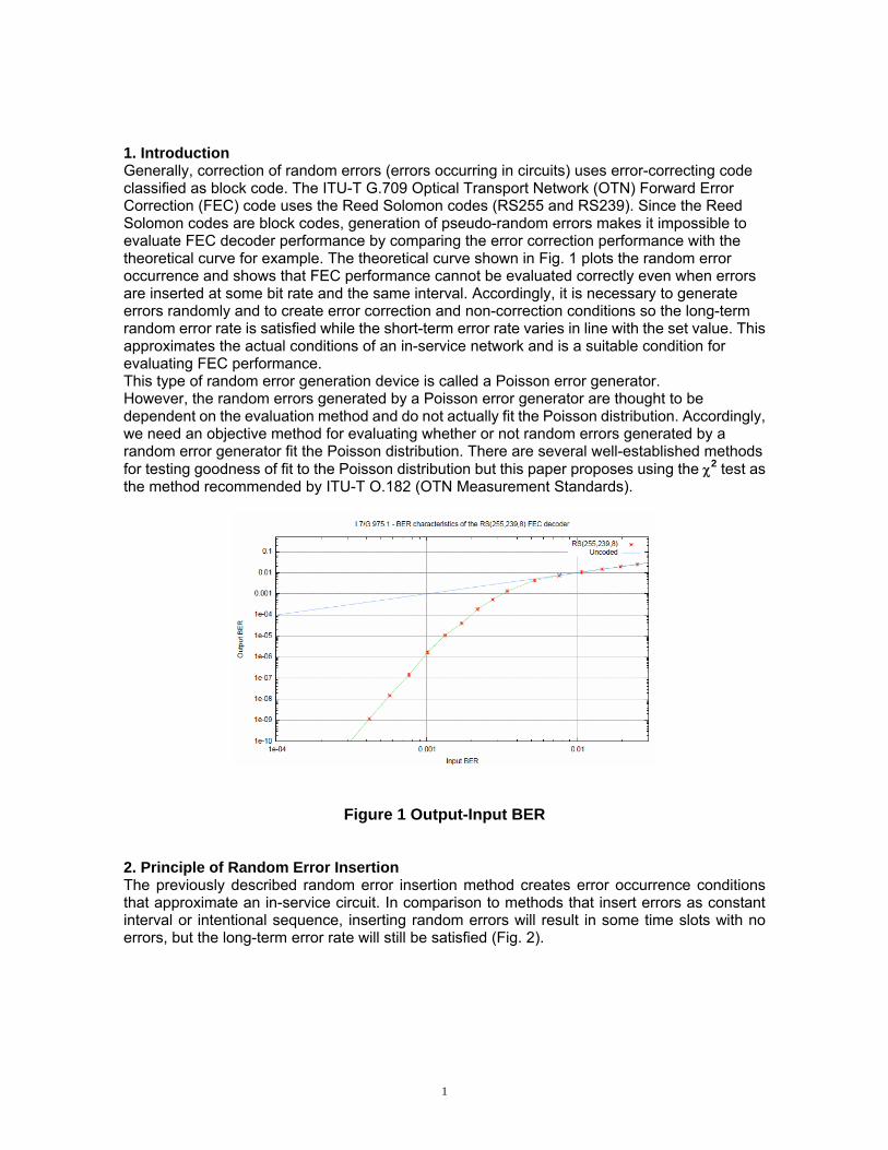
1. Introduction Generally, correction of random errors (errors occurring in circuits) uses error-correcting code classified as block code. The ITU-T G.709 Optical Transport Network (OTN) Forward Error Correction (FEC) code uses the Reed Solomon codes (RS255 and RS239). Since the Reed Solomon codes are block codes, generation of pseudo-random errors makes it impossible to evaluate FEC decoder performance by comparing the error correction performance with the theoretical curve for example. The theoretical curve shown in Fig. 1 plots the random error occurrence and shows that FEC performance cannot be evaluated correctly even when errors are inserted at some bit rate and the same interval. Accordingly, it is necessary to generate errors randomly and to create error correction and non-correction conditions so the long-term random error rate is satisfied while the short-term error rate varies in line with the set value. This approximates the actual conditions of an in-service network and is a suitable condition for evaluating FEC performance. This type of random error generation device is called a Poisson error generator. However, the random errors generated by a Poisson error generator are thought to be dependent on the evaluation method and do not actually fit the Poisson distribution. Accordingly, we need an objective method for evaluating whether or not random errors generated by a random error generator fit the Poisson distribution. There are several well-established methods for testing goodness of fit to the Poisson distribution but this paper proposes using the χ2 test as the method recommended by ITU-T O.182 (OTN Measurement Standards).

Figure 1 Output-Input BER

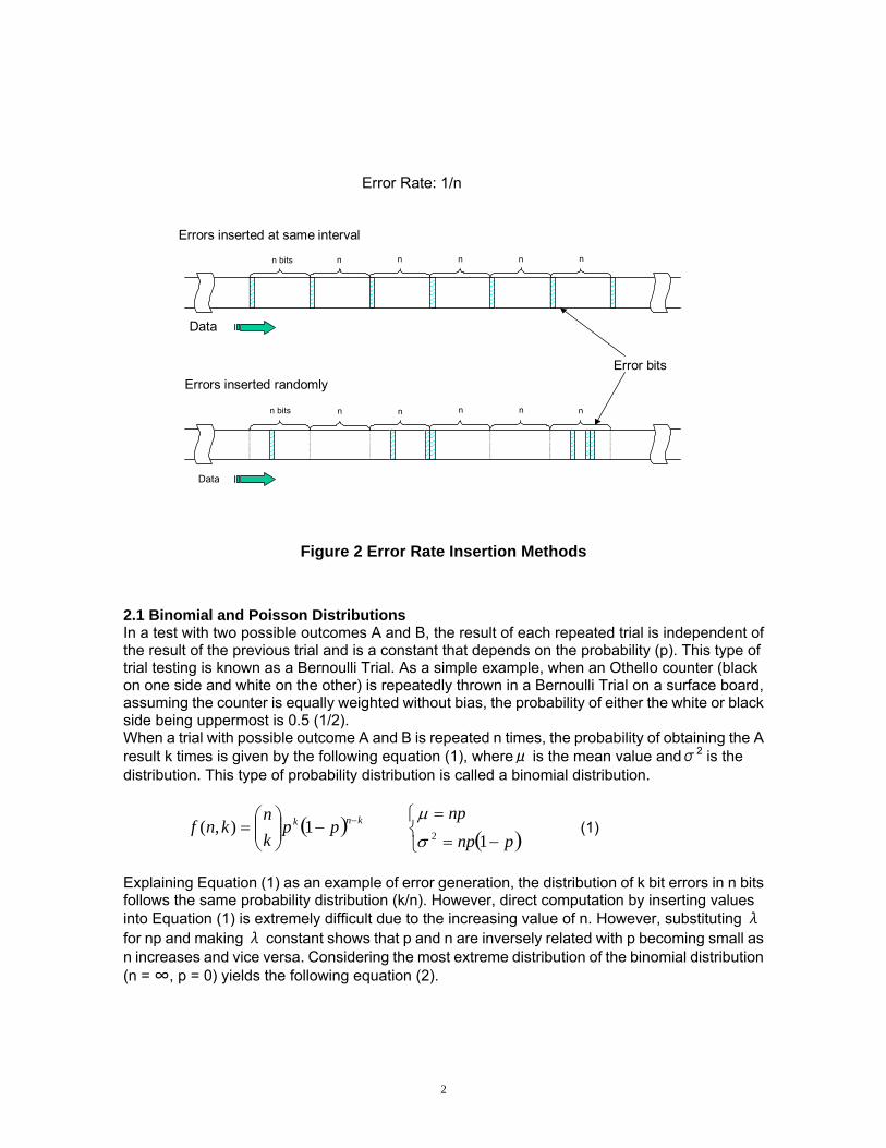
2. Principle of Random Error Insertion The previously described random error insertion method creates error occurrence conditions that approximate an in-service circuit. In comparison to methods that insert errors as constant interval or intentional sequence, inserting random errors will result in some time slots with no errors, but the long-term error rate will still be satisfied (Fig. 2).

2

Errors inserted at same interval Errors

inserted at same intervalError Rate: 1/n

n bits

Errors inserted at same interval

Errors inserted randomly Error bits

Error Rate: 1/n

Data

Data

n n n n n

n bits n n n n n

Figure 2 Error Rate Insertion Methods

2.1 Binomial and Poisson Distributions In a test with two possible outcomes A and B, the result of each repeated trial is independent of the result of the previous trial and is a constant that depends on the probability (p). This type of trial testing is known as a Bernoulli Trial. As a simple example, when an Othello counter (black on one side and white on the other) is repeatedly thrown in a Bernoulli Trial on a surface board, assuming the counter is equally weighted without bias, the probability of either the white or black side being uppermost is 0.5 (1/2). When a trial with possible outcome A and B is repeated n times, the probability of obtaining the A result k times is given by the following equation (1), whereμ is the mean value andσ2 is the distribution. This type of probability distribution is called a binomial distribution.

( ) knk ppkn

knf −−⎟⎟⎠

⎞⎜⎜⎝

⎛= 1),(

( )⎩⎨⎧

−=

=

pnpnp

12σ

μ (1)

Explaining Equation (1) as an example of error generation, the distribution of k bit errors in n bits follows the same probability distribution (k/n). However, direct computation by inserting values into Equation (1) is extremely difficult due to the increasing value of n. However, substituting λfor np and making λ constant shows that p and n are inversely related with p becoming small as n increases and vice versa. Considering the most extreme distribution of the binomial distribution (n = ∞, p = 0) yields the following equation (2).

3

( )!

;k

ekfkλλ λ−=

⎩⎨⎧

=

=

λσ

λμ2 (2)

The probability distribution given by Equation (2) is called the Poisson distribution. Since λ is a fixed value, the distribution is expressed by the variable k. Due to the relationship between the Poisson and binomial distributions, substituting np for λ yields

( )!)(; )(

knpenpkf

knp−= (3)

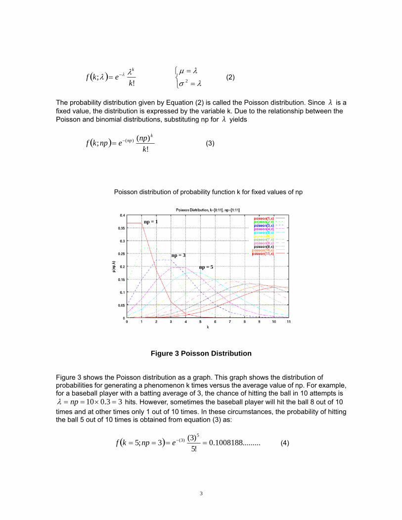
Figure 3 Poisson Distribution

Figure 3 shows the Poisson distribution as a graph. This graph shows the distribution of probabilities for generating a phenomenon k times versus the average value of np. For example, for a baseball player with a batting average of 3, the chance of hitting the ball in 10 attempts is

33.010 =×== npλ hits. However, sometimes the baseball player will hit the ball 8 out of 10 times and at other times only 1 out of 10 times. In these circumstances, the probability of hitting the ball 5 out of 10 times is obtained from equation (3) as:

( ) .........1008188.0!5)3(3;5

5)3( ==== −enpkf (4)

Poisson distribution of probability function k for fixed values of np

np = 3

np = 1

np = 5

4

In other words, there is about a 10% chance of hitting the ball 5 out of 10 times. This result is the probability distribution expressed by “poisson(3,x)” in Figure 3. Using the “poisson(3,x)” plot, since this player hits with an average of 3, the peak of the plot is at k = 3 and the probability of getting 3 out of 10 hits is 22.4%. In addition, we can see that the probability drops whether the hit count rises or falls. 2.2 Poisson Distribution and Error Rate

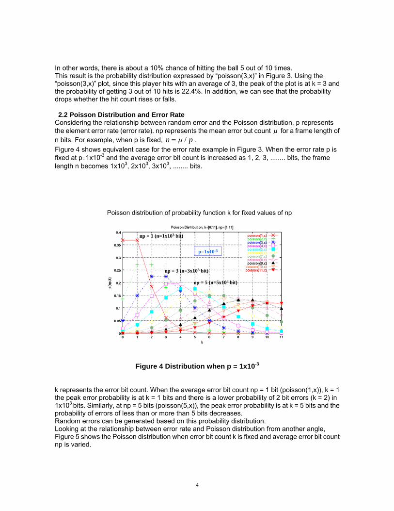
Considering the relationship between random error and the Poisson distribution, p represents the element error rate (error rate). np represents the mean error but count μ for a frame length of n bits. For example, when p is fixed, pn /μ= . Figure 4 shows equivalent case for the error rate example in Figure 3. When the error rate p is fixed at p：1x10-3 and the average error bit count is increased as 1, 2, 3, ........ bits, the frame length n becomes 1x103, 2x103, 3x103, ........ bits.

Figure 4 Distribution when p = 1x10-3

k represents the error bit count. When the average error bit count np = 1 bit (poisson(1,x)), k = 1 the peak error probability is at k = 1 bits and there is a lower probability of 2 bit errors (k = 2) in 1x103 bits. Similarly, at np = 5 bits (poisson(5,x)), the peak error probability is at k = 5 bits and the probability of errors of less than or more than 5 bits decreases. Random errors can be generated based on this probability distribution. Looking at the relationship between error rate and Poisson distribution from another angle, Figure 5 shows the Poisson distribution when error bit count k is fixed and average error bit count np is varied.

Poisson distribution of probability function k for fixed values of np

np = 1 (n=1x103 bit)

np = 3 (n=3x103 bit)

np = 5 (n=5x103 bit)

p=1x10-3

5

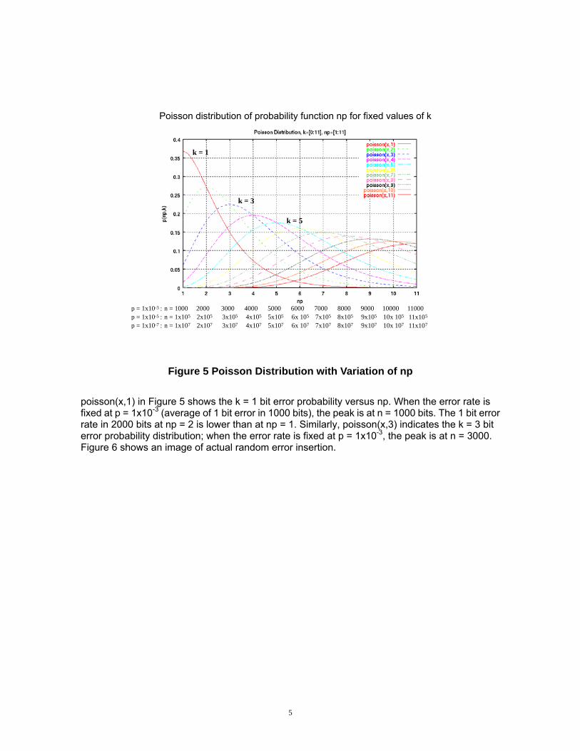
Figure 5 Poisson Distribution with Variation of np

poisson(x,1) in Figure 5 shows the k = 1 bit error probability versus np. When the error rate is fixed at p = 1x10-3 (average of 1 bit error in 1000 bits), the peak is at n = 1000 bits. The 1 bit error rate in 2000 bits at np = 2 is lower than at np = 1. Similarly, poisson(x,3) indicates the k = 3 bit error probability distribution; when the error rate is fixed at p = 1x10-3, the peak is at n = 3000. Figure 6 shows an image of actual random error insertion.

Poisson distribution of probability function np for fixed values of k

p = 1x10-3 : n = 1000 2000 3000 4000 5000 6000 7000 8000 9000 10000 11000 p = 1x10-5 : n = 1x105 2x105 3x105 4x105 5x105 6x 105 7x105

8x105 9x105 10x 105 11x105 p = 1x10-7 : n = 1x107 2x107 3x107 4x107 5x107 6x 107 7x107 8x107 9x107 10x 107 11x107

k = 1

k = 3

k = 5

6

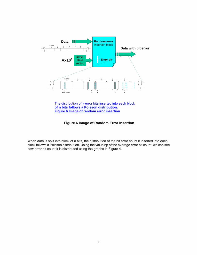
Figure 6 Image of Random Error Insertion

When data is split into block of n bits, the distribution of the bit error count k inserted into each block follows a Poisson distribution. Using the value np of the average error bit count, we can see how error bit count k is distributed using the graphs in Figure 4.

Random errorinsertion block

Data n n n n nn bits

ErrorRate

settingAx10 -B

Data with bit error

n n bits n n n n

k Bit Error kkk k

=

Error bit

The distribution of k error bits inserted into each blockof n bits follows a Poisson distribution. Figure 6 Image of random error insertion

7

3． Applicability of χ2 Test to Poisson Distribution Goodness of Fit Sometimes, the random error generator called a Poisson Error Generator does not generate errors fitting the Poisson distribution. Consequently, we require an objective method for evaluating the distribution of random errors generated by the random error generator. The methods for evaluating probability distributions are called tests of goodness of fit and objectively evaluate whether the obtained probability distribution matches the hypothesis. There are several goodness of fit test methods but this White Paper explains the χ2 Test of Goodness of Fit used by ITU-T O.182 (OTN Measurement Standards). The χ2 test is described as a hypothesis test because it tests whether or not the sample of finite observed data accurately describes the hypothesis. The χ2 test is one of many hypothesis methods for testing goodness of fit but it is a typical method. Like other test methods, the χ2 test is not a universal test for goodness of fit and it be used for all distributions. Fortunately, however, it is one of the best methods for testing the goodness of fit for Poisson distribution and is frequently used when the assumed distribution is a Poisson distribution. As already mentioned, λ, the only parameter of the Poisson distribution can be chosen freely by determining any value for the observation time n. Actually, when testing goodness of fit to the Poisson distribution, the optimum value for λ is given by the following relationship.

5 ≤ λ ≤ 20 (5) It is especially important to satisfy the lower limit of the formula. On the other hand, the upper limit does not always need to be satisfied because it is obtained from the observation time limit. If the situation permits, λ does not necessarily need to be restricted by the upper limit of (5) if no problems are caused by increasing the observation time. When the value of λ is small, the Poisson distribution is skewed to the left and the number of observations is reduced as a result. Here, the observed frequency k is the error occurrence frequency (including 0) for observation time n. The details of the observed frequency are explained later. When testing goodness of fit, the number of observed items should be at least 5. Although this value is based on empirical evidence, it is necessary to maintain the reliability of the result of the hypothesis test at a fixed level. In fact, since the χ2 test is based on large sample theory, small sample sizes reduce the test reliability. On the other hand, if the value of λ is larger than necessary, the number of observations increases as a result while the frequency of each item becomes small. Of course, although the frequency of each item can be increased by increasing the number of observations, the observation time also increases as a result. When testing goodness of fit using the χ2 test, the frequency of each item should be at least 5. This is another limitation on using the χ2 test that is required to maintain the reliability of the goodness of fit test result at a fixed level.

8

4. Principle of χ2 Test Letting jfff ,,, 21 L and jeee ,,, 21 L be the observed frequency and expected frequency for N experiments where j is the number of possible outcomes, the value given by the equation

∑=

−=

j

i i

ii

eef

1

22 )(χ (6)

approaches the χ2 distribution for ν = j − 1− t degrees of freedom as N increases where t is the number of estimated parameters. Generally, when testing goodness of fit for the Poisson distribution, the parameter λ is estimated from the sample, so degrees of freedom ν = j – 2. From equation (6), it is clear that χ2 becomes smaller as the observed sample fits the proposed hypothesis. Normally, this never happens but if the value of χ2 のfound by the above equation became 0, it would indicate a perfect match between the distribution of the observed sample and the hypothetical distribution. The test of goodness of fit using the χ2 test is a method for testing the hypothesis based on the value of χ2 found by the above equation. Furthermore, since the χ2 distribution is equivalent to when α = ν/2, andβ = 2 in the gamma distribution, therefore,

⎪⎩

⎪⎨⎧

<

≥Γ==

−−

0,0

0,)2/(2)()( 2/

2/12/

2

x

xexxGax

x

νχ ν

ν

（7）

where ν is the degrees of freedom of the χ2 distribution. Moreover, )(αΓ is the gamma function given by the following equation.

dxex x−∞ −∫=Γ0

1)( αα (8)

Since Γ(α+ 1) = αΓ(α), when α is an integer value, Γ(α +1) = α! And the value of the gamma functions can be factoring, explaining why the gamma function is sometimes called a factorial function. Moreover, since the χ2 distribution function is also a probability density function, the function area approaches 1, meaning

1)(0

2 =∫∞

dxxχ (9)

Calculating the area of the right tail from some point χα

of the χ2 distribution (representing the incomplete integration as α), then

dxx)(2

2∫∞

=αχχα (10)

Because the entire area of the χ2 distribution function is 1, the value of α given by the above equation represents the area ratio and α is called the significance level. Generally, significance is expressed as a percentage obtained by multiplying α by 100 and this White Paper follows the same convention. Since the χ2 distribution is a monotonous and continuous function, χ2

α can be found from the significance level 100 x α and is called the significance point, critical point, or percent point.

9

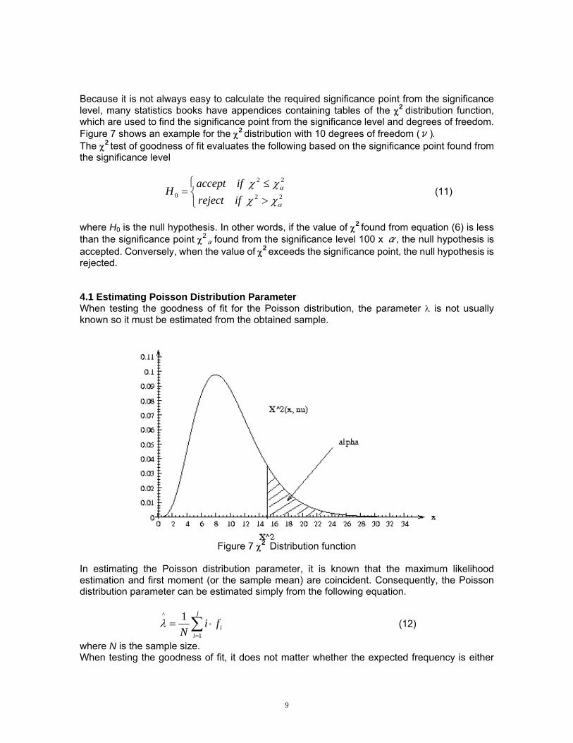
Because it is not always easy to calculate the required significance point from the significance level, many statistics books have appendices containing tables of the χ2 distribution function, which are used to find the significance point from the significance level and degrees of freedom. Figure 7 shows an example for the χ2 distribution with 10 degrees of freedom (ν). The χ2 test of goodness of fit evaluates the following based on the significance point found from the significance level

⎩⎨⎧

>≤

= 22

22

0α

α

χχχχ

ifrejectifaccept

H (11)

where H0 is the null hypothesis. In other words, if the value of χ2 found from equation (6) is less than the significance point χ2

α found from the significance level 100 x α, the null hypothesis is accepted. Conversely, when the value of χ2 exceeds the significance point, the null hypothesis is rejected. 4.1 Estimating Poisson Distribution Parameter When testing the goodness of fit for the Poisson distribution, the parameter λ is not usually known so it must be estimated from the obtained sample.

Figure 7 χ2 Distribution function

In estimating the Poisson distribution parameter, it is known that the maximum likelihood estimation and first moment (or the sample mean) are coincident. Consequently, the Poisson distribution parameter can be estimated simply from the following equation.

∑=

⋅=j

iifi

N 1

^ 1λ (12)

where N is the sample size. When testing the goodness of fit, it does not matter whether the expected frequency is either

10

calculated from this parameter, or estimated from the observed sample. The k-th probability pk for the Poisson distribution calculated based on the determined value of λ is found from the following equation.

!

^^

kep

k

kλλ−= (13)

And the k-th expected frequency is given by

kk pNe ⋅= (14)

5. Examples of Poisson Distribution Goodness of Fit This section explains two examples of Poisson distribution goodness of fit. The first example shows a fit at the 5% significance level while the second shows an example that does not a fit at the 5% significance level.

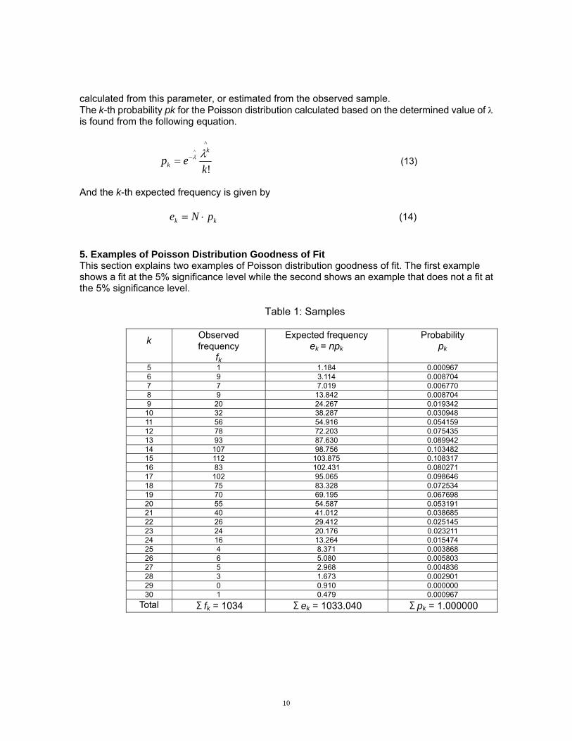
Table 1: Samples

k Observed frequency

fk

Expected frequency ek = npk

Probability pk

5 1 1.184 0.000967 6 9 3.114 0.008704 7 7 7.019 0.006770 8 9 13.842 0.008704 9 20 24.267 0.019342

10 32 38.287 0.030948 11 56 54.916 0.054159 12 78 72.203 0.075435 13 93 87.630 0.089942 14 107 98.756 0.103482 15 112 103.875 0.108317 16 83 102.431 0.080271 17 102 95.065 0.098646 18 75 83.328 0.072534 19 70 69.195 0.067698 20 55 54.587 0.053191 21 40 41.012 0.038685 22 26 29.412 0.025145 23 24 20.176 0.023211 24 16 13.264 0.015474 25 4 8.371 0.003868 26 6 5.080 0.005803 27 5 2.968 0.004836 28 3 1.673 0.002901 29 0 0.910 0.000000 30 1 0.479 0.000967

Total Σfk = 1034 Σek = 1033.040 Σpk = 1.000000

11

Both examples are obtained from an actual Poisson error generator under the same conditions with an element error rate pe = 10-8 and sample size N > 1000. Furthermore, in both examples, the number of average errors occurring in the observation time n was chosen so that λ = 16. In other words, the experiment was executed with observation time n = λ/ pe. Incidentally, observation time means discrete time (number of actual clocks).

12

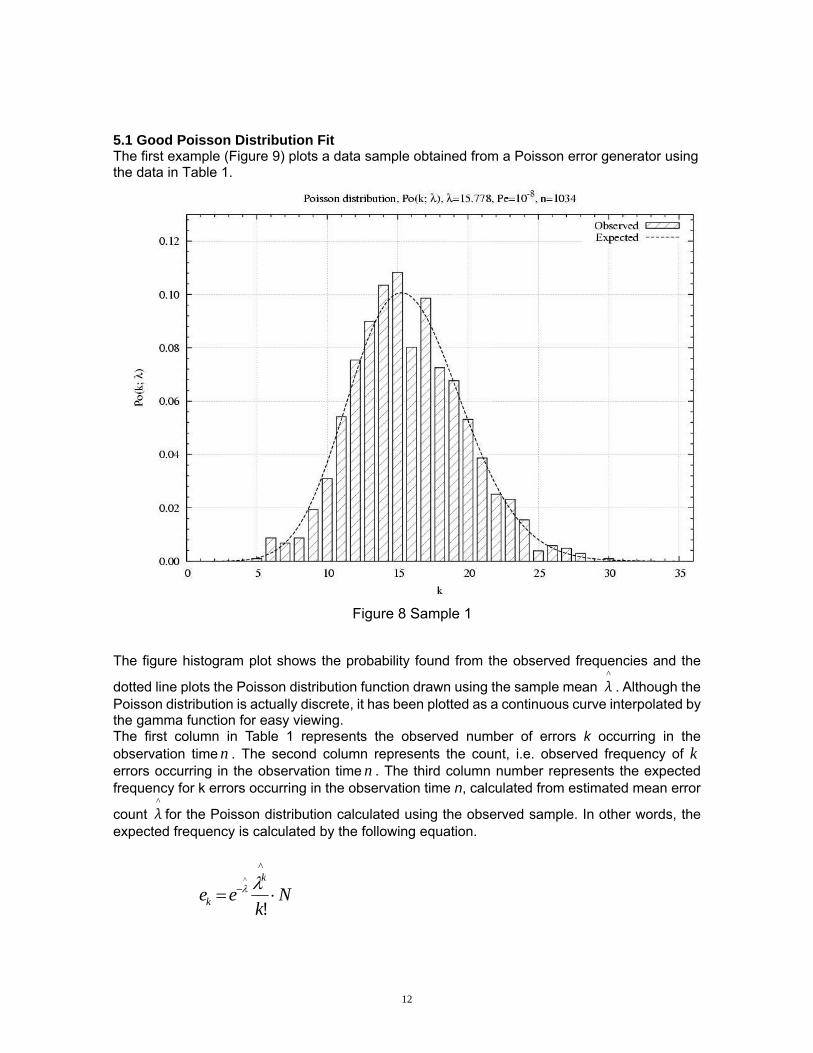
5.1 Good Poisson Distribution Fit The first example (Figure 9) plots a data sample obtained from a Poisson error generator using the data in Table 1.

Figure 8 Sample 1

The figure histogram plot shows the probability found from the observed frequencies and the

dotted line plots the Poisson distribution function drawn using the sample mean λ^

. Although the Poisson distribution is actually discrete, it has been plotted as a continuous curve interpolated by the gamma function for easy viewing. The first column in Table 1 represents the observed number of errors k occurring in the observation time n . The second column represents the count, i.e. observed frequency of k errors occurring in the observation time n . The third column number represents the expected frequency for k errors occurring in the observation time n, calculated from estimated mean error

count λ^

for the Poisson distribution calculated using the observed sample. In other words, the expected frequency is calculated by the following equation.

Nk

eek

k ⋅= −

!

^^ λλ

13

where N is the sample size. The fourth column represents the probability of k errors occurring in the observation time n. This probability is found easily from the following equation.

Nfp kk /= The bottom row shows the sum for each column. The sum of the second column is sum of the observed frequency, and is also the sample size N. The sum of the third column is the sum of the expected frequency.

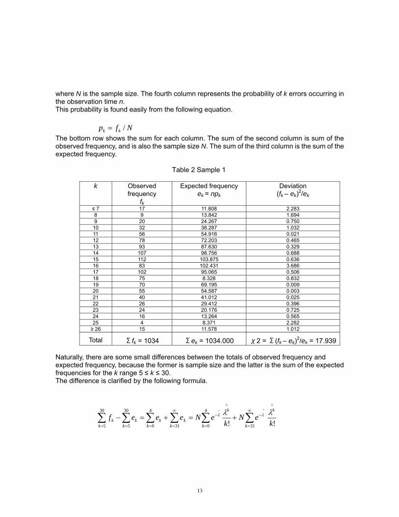
Table 2 Sample 1

k Observed frequency

fk

Expected frequency ek = npk

Deviation (fk – ek)2/ek

≤ 7 17 11.808 2.283 8 9 13.842 1.694 9 20 24.267 0.750

10 32 38.287 1.032 11 56 54.916 0.021 12 78 72.203 0.465 13 93 87.630 0.329 14 107 98.756 0.688 15 112 103.875 0.636 16 83 102.431 3.686 17 102 95.065 0.506 18 75 8.328 0.832 19 70 69.195 0.009 20 55 54.587 0.003 21 40 41.012 0.025 22 26 29.412 0.396 23 24 20.176 0.725 24 16 13.264 0.565 25 4 8.371 2.282 ≥ 26 15 11.578 1.012

Total Σfk = 1034 Σek = 1034.000 χ2 = Σ(fk – ek)2/ek = 17.939 Naturally, there are some small differences between the totals of observed frequency and expected frequency, because the former is sample size and the latter is the sum of the expected frequencies for the k range 5 ≤ k ≤ 30. The difference is clarified by the following formula.

!!

^

31

^4

031

4

0

30

5

30

5

^^

keN

keNeeef

k

k

k

kkk

kk

k kkk

λλ λλ ∑∑∑∑∑ ∑∞

=

−

=

−∞

=== =

+=+=−

14

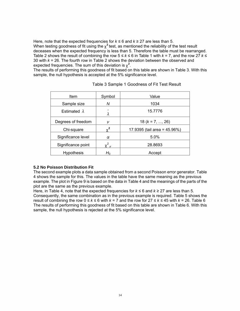
Here, note that the expected frequencies for k ≤ 6 and k ≥ 27 are less than 5. When testing goodness of fit using the χ2 test, as mentioned the reliability of the test result deceases when the expected frequency is less than 5. Therefore the table must be rearranged. Table 2 shows the result of combining the row 5 ≤ k ≤ 6 in Table 1 with k = 7, and the row 27 k ≤ 30 with k = 26. The fourth row in Table 2 shows the deviation between the observed and expected frequencies. The sum of this deviation is χ2. The results of performing this goodness of fit based on this table are shown in Table 3. With this sample, the null hypothesis is accepted at the 5% significance level.

Table 3 Sample 1 Goodness of Fit Test Result

Item Symbol Value

Sample size N 1034

Estimated λ λ

^

15.7776

Degrees of freedom ν 18 (k = 7, ..., 26)

Chi-square χ2 17.9395 (tail area = 45.96%)

Significance level α 5.0%

Significance point χ2α 28.8693

Hypothesis H0 Accept

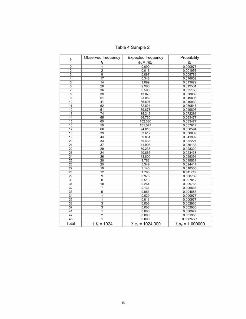
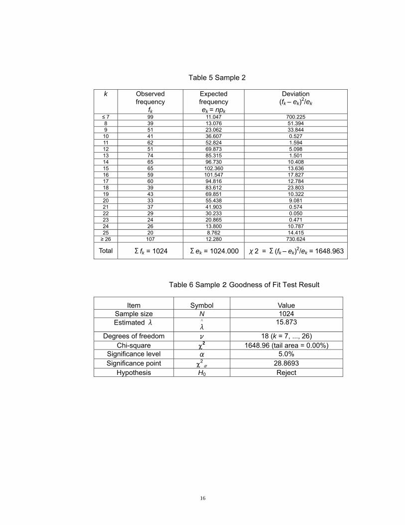
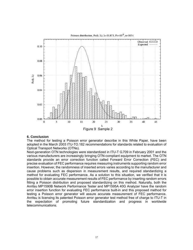
5.2 No Poisson Distribution Fit The second example plots a data sample obtained from a second Poisson error generator. Table 4 shows the sample for this. The values in the table have the same meaning as the previous example. The plot in Figure 9 is based on the data in Table 4 and the meanings of the parts of the plot are the same as the previous example. Here, in Table 4, note that the expected frequencies for k ≤ 6 and k ≥ 27 are less than 5. Consequently, the same combination as in the previous example is required. Table 5 shows the result of combining the row 0 ≤ k ≤ 6 with k = 7 and the row for 27 ≤ k ≤ 45 with k = 26. Table 6 The results of performing this goodness of fit based on this table are shown in Table 6. With this sample, the null hypothesis is rejected at the 5% significance level.

15

Table 4 Sample 2

k Observed frequencyfk

Expected frequency ek = npk

Probability pk

0 1 0.000 0.000977 2 2 0.016 0.001953 3 9 0.087 0.008789 4 17 0.346 0.016602 5 14 1.099 0.013672 6 20 2.906 0.019531 7 36 6.590 0.035156 8 39 13.076 0.038089 9 51 23.062 0.049805

10 41 36.607 0.040039 11 62 52.824 0.060547 12 51 69.873 0.049805 13 74 85.315 0.072266 14 65 96.730 0.063477 15 65 102.360 0.063477 16 59 101.547 0.057617 17 60 94.816 0.058594 18 39 83.612 0.038089 19 43 69.851 0.041992 20 33 55.438 0.032227 21 37 41.903 0.036133 22 29 30.233 0.028320 23 24 20.865 0.023438 24 26 13.800 0.025391 25 20 8.762 0.019531 26 25 5.349 0.024414 27 19 3.145 0.018555 28 12 1.783 0.011719 29 9 0.976 0.008789 30 8 0.516 0.007812 31 10 0.264 0.009766 32 7 0.131 0.006836 33 5 0.063 0.004883 34 1 0.029 0.000977 35 1 0.013 0.000977 36 3 0.006 0.002930 37 3 0.003 0.002930 41 1 0.000 0.000977 42 2 0.000 0.001953 45 1 0.000 0.0009777

Total Σfk = 1024 Σek = 1024.000 Σpk = 1.000000

16

Table 5 Sample 2

k Observed

frequency fk

Expected frequency ek = npk

Deviation (fk – ek)2/ek

≤ 7 99 11.047 700.225 8 39 13.076 51.394 9 51 23.062 33.844

10 41 36.607 0.527 11 62 52.824 1.594 12 51 69.873 5.098 13 74 85.315 1.501 14 65 96.730 10.408 15 65 102.360 13.636 16 59 101.547 17.827 17 60 94.816 12.784 18 39 83.612 23.803 19 43 69.851 10.322 20 33 55.438 9.081 21 37 41.903 0.574 22 29 30.233 0.050 23 24 20.865 0.471 24 26 13.800 10.787 25 20 8.762 14.415 ≥ 26 107 12.280 730.624

Total Σfk = 1024 Σek = 1024.000 χ2 = Σ(fk – ek)2/ek = 1648.963

Table 6 Sample ２ Goodness of Fit Test Result

Item Symbol Value Sample size N 1024 Estimated λ

λ^

15.873

Degrees of freedom ν 18 (k = 7, ..., 26) Chi-square χ2 1648.96 (tail area = 0.00%)

Significance level α 5.0% Significance point χ2

α 28.8693 Hypothesis H0 Reject

17

Figure 9 Sample 2

6. Conclusion The method for testing a Poisson error generator describe in this White Paper, have been adopted in the March 2003 ITU-TO.182 recommendations for standards related to evaluation of Optical Transport Networks (OTNs). Next-generation OTN technologies were standardized in ITU-T G.709 in February 2001 and the various manufacturers are increasingly bringing OTN-compliant equipment to market. The OTN standards provide an error correction function called Forward Error Correction (FEC) and precise evaluation of FEC performance requires measuring instruments supporting random error insertion. However, the randomness of inserted errors varies according to the manufacturer and cause problems such as dispersion in measurement results, and required standardizing a method for evaluating FEC performance. As a solution to this situation, we verified that it is possible to obtain accurate measurement results of FEC performance by inserting random errors fitting a Poisson distribution and proposed standardizing on this method. Naturally, both the Anritsu MP1590B Network Performance Tester and MP1595A 40G Analyzer have the random error insertion function for evaluating FEC performance built-in and this proposed method for testing a Poisson error generator will assure accurate measurement of FEC performance. Anritsu is licensing its patented Poisson error generator test method free of charge to ITU-T in the expectation of promoting future standardization and progress in worldwide telecommunications.

18

References [1] Paul G. Hoel, “Introduction to Mathematical Statistics,” John Wiley & Sons, 1984. [2] George P. Wadsworth and Joseph G. Bryan, “Applications of Probability and Random Variables,” McGraw-Hill, Inc., 1974. [3] Harald Cram´er, “Mathematical Methods of Statistics,” Princeton University Press, Princeton, New Jersey, 1974. [4] Abramowitz and Stegun, “Handbook of Mathematical Functions,” National Bureau of Standards, 1970. [5] William H. Press, Saul A. Teukolsky, William T. Vetterling, and Brian P. Flannery. “Numerical Recipes in C,” Cambridge University Press, 1992.

Anritsu Corporation5-1-1 Onna, Atsugi-shi, Kanagawa, 243-8555 JapanPhone: +81-46-223-1111Fax: +81-46-296-1264

• U.S.A.Anritsu Company1155 East Collins Blvd., Suite 100, Richardson, TX 75081, U.S.A.Toll Free: 1-800-267-4878Phone: +1-972-644-1777Fax: +1-972-671-1877

• CanadaAnritsu Electronics Ltd.700 Silver Seven Road, Suite 120, Kanata, Ontario K2V 1C3, CanadaPhone: +1-613-591-2003 Fax: +1-613-591-1006

• Brazil Anritsu Eletrônica Ltda.Praca Amadeu Amaral, 27 - 1 Andar01327-010-Paraiso-São Paulo-BrazilPhone: +55-11-3283-2511Fax: +55-11-3288-6940

• U.K.Anritsu EMEA Ltd.200 Capability Green, Luton, Bedfordshire, LU1 3LU, U.K.Phone: +44-1582-433200 Fax: +44-1582-731303

• FranceAnritsu S.A.9 Avenue du Québec, Z.A. de Courtabœuf 91951 Les Ulis Cedex, France Phone: +33-1-60-92-15-50Fax: +33-1-64-46-10-65

• GermanyAnritsu GmbHNemetschek Haus, Konrad-Zuse-Platz 1 81829 München, Germany Phone: +49-89-442308-0 Fax: +49-89-442308-55

• ItalyAnritsu S.p.A.Via Elio Vittorini 129, 00144 Roma, ItalyPhone: +39-6-509-9711 Fax: +39-6-502-2425

• SwedenAnritsu ABBorgafjordsgatan 13, 164 40 KISTA, SwedenPhone: +46-8-534-707-00 Fax: +46-8-534-707-30

• FinlandAnritsu ABTeknobulevardi 3-5, FI-01530 VANTAA, FinlandPhone: +358-20-741-8100Fax: +358-20-741-8111

• DenmarkAnritsu A/SKirkebjerg Allé 90, DK-2605 Brøndby, DenmarkPhone: +45-72112200Fax: +45-72112210

• SpainAnritsu EMEA Ltd. Oficina de Representación en EspañaEdificio VeganovaAvda de la Vega, n˚ 1 (edf 8, pl 1, of 8)28108 ALCOBENDAS - Madrid, SpainPhone: +34-914905761Fax: +34-914905762

• United Arab EmiratesAnritsu EMEA Ltd.Dubai Liaison OfficeP O Box 500413 - Dubai Internet CityAl Thuraya Building, Tower 1, Suit 701, 7th FloorDubai, United Arab EmiratesPhone: +971-4-3670352Fax: +971-4-3688460

• SingaporeAnritsu Pte. Ltd.10, Hoe Chiang Road, #07-01/02, Keppel Towers,Singapore 089315 Phone: +65-6282-2400 Fax: +65-6282-2533

• IndiaAnritsu Pte. Ltd. India Branch OfficeUnit No. S-3, Second Floor, Esteem Red Cross Bhavan,No. 26, Race Course Road, Bangalore 560 001, IndiaPhone: +91-80-32944707Fax: +91-80-22356648

• P.R. China (Hong Kong)Anritsu Company Ltd.Units 4 & 5, 28th Floor, Greenfield Tower, Concordia Plaza, No. 1 Science Museum Road, Tsim Sha Tsui East,Kowloon, Hong KongPhone: +852-2301-4980Fax: +852-2301-3545

• P.R. China (Beijing)Anritsu Company Ltd.Beijing Representative OfficeRoom 1515, Beijing Fortune Building, No. 5, Dong-San-Huan Bei Road, Chao-Yang District, Beijing 10004, P.R. ChinaPhone: +86-10-6590-9230Fax: +86-10-6590-9235

• KoreaAnritsu Corporation, Ltd.8F Hyunjuk Building, 832-41, Yeoksam Dong, Kangnam-ku, Seoul, 135-080, KoreaPhone: +82-2-553-6603Fax: +82-2-553-6604

• AustraliaAnritsu Pty. Ltd.Unit 21/270 Ferntree Gully Road, Notting Hill, Victoria 3168, AustraliaPhone: +61-3-9558-8177Fax: +61-3-9558-8255

• TaiwanAnritsu Company Inc.7F, No. 316, Sec. 1, Neihu Rd., Taipei 114, TaiwanPhone: +886-2-8751-1816Fax: +886-2-8751-1817

Specifications are subject to change without notice.

No. MP1591A_FEC-E-R-1-(1.00） Printed in Japan 2007-4 AKD

Please Contact:

070207

Printed on 70% Recycled Paper