Effect of Material Texture on fatigue crack growth and fracture toughness
Fatigue design of steel and
composite bridges
MOHAMMAD AL-EMRANI MUSTAFA AYGÜL Department of Civil and Environmental Engineering Division of Structural Engineering Steel and Timber Structures CHALMERS UNIVERSITY OF TECHNOLOGY Göteborg, Sweden 2014 Report 2014:10
Dσ∆
Lσ∆
in
σ∆

REPORT 2014:10
Error! Reference source not found.
MOHAMMAD AL-EMRANI
Department of Civil and Environmental Engineering Division of Structural Engineering
Steel and Timber Structures
CHALMERS UNIVERSITY OF TECHNOLOGY
Göteborg, Sweden 2014

Fatigue design of steel and composite bridges
MOHAMMAD AL-EMRANI
© MOHAMMAD AL-EMRANI AND MUSTAFA AYGÜL, 2014
Chalmers tekniska högskola 2014: ISSN 1652-9162 Department of Civil and Environmental Engineering Division of Structural Engineering STEEL AND TIMBER STRUCTURES Chalmers University of Technology SE-412 96 Göteborg Sweden Telephone: + 46 (0)31-772 1000 Chalmers Reproservice, Göteborg, Sweden 2014
CHALMERS Civil and Environmental Engineering, Report 2014:10 V
Preface
This report has been produced within the research project “Methods for the fatigue design of steel and composite bridges” which was funded by the Swedish Road Administration, Trafikverket. The authors would like to express their gratitude to the following persons who have followed up and supported the work in the project and contributed with valuable comments and suggestions to this report:
Lahja Rydberg-Forssbeck Trafikverket
Robert Hällmark Trafikverket
Kurt Palmqvist Trafikverket
In addition, parts of the recommendations and guidelines presented in this report where based on previous extensive research in the field of fatigue of welded connections conducted within other research projects and in various master’s thesis projects. The authors are most thankful for the contributions of the following colleagues to the work:
Mohsen Heshmati Chalmers
Farshid Zamiri Chalmers / EPFL-Switzerland
Göteborg, November 2014
Mohammad Al-Emrani & Mustafa Aygul

CHALMERS, Civil and Environmental Engineering, Report 2014:10 VI

CONTENTS
1 INTRODUCTION 1
1.1 Eurocodes for bridge design 1
1.2 Application areas and limitations 3
1.2.1 Material 3
1.2.2 Temperature 3
1.2.3 Corrosion 3
1.2.4 General procedure for using the methodsError! Bookmark not
defined.
2 FATIGUE LOAD MODELS IN EUROCODE 4
2.1 Fatigue load models for road bridges 6
2.1.1 Fatigue load model 1, FLM1 7
2.1.2 Fatigue load model 2, FLM2 8
2.1.3 Fatigue load model 3, FLM 3 9
2.1.4 Fatigue load model 4, FLM 4 11
2.1.5 Fatigue load model 5, FLM 5 15
2.1.6 Summary 16
2.2 Fatigue load models for railway bridges 16
2.2.1 Fatigue load models for the λ-coefficient method 17
2.2.2 Fatigue load models for the cumulative damage method 18
2.2.3 Summary 21
3 FATIGUE DESIGN METHODS 23
3.1 The concept of Equivalent Stress Range 23
3.2 Fatigue design with the λ-coefficient method 24
3.2.1 Factor λ1 27
3.2.2 Factor λ2 29
3.2.3 Factor λ3 31
3.2.4 Factor λ4 32
3.2.5 Factor λmax 33
3.3 Fatigue design with the Damage Accumulation Method 35
3.4 Palmgren-Miner damage accumulation 36
3.5 The application of Equivalent Stress Range 37
3.6 The application of the damage accumulation method 40
3.7 Application to road bridges 40
3.8 Application for railway bridges 45
4 WORKED EXAMPLES 48
4.1 Fatigue design of a road Bridge 48
4.1.1 General description 48
4.1.2 Concrete deck 49
CHALMERS, Civil and Environmental Engineering, Report 2014:10 II
4.1.3 Fatigue verification using the simplified λ-method 53
4.1.4 Fatigue verification using the Damage Accumulation method 58
4.2 Worked example – fatigue design of a railway bridge 66
4.2.1 Description of the bridge 66
4.2.2 Bridge specific traffic data 67
4.2.3 Fatigue verification using the simplified λ-method 67
4.3 Fatigue verification using the Damage Accumulation method 72
4.3.1 Traffic load models 73
4.3.2 Bridge response to train load models 73
5 FATIGUE DESIGN USING THE STRUCTURAL HOT-SPOT STRESS
METHOD 81
5.1 Introduction 81
5.2 Principals of the structural hot-spot stress method 84
5.3 Structural hot-spot stress determination in welded details 85
5.3.1 The determination of the structural hot-spot stress using FEM 86
5.3.2 Determination of the structural hot-spot stress from measurements 90
5.3.3 Determination of the structural hot-spot stress in biaxial stress state 91
5.4 Fatigue verification with the structural hot-spot stress method 92
5.4.1 Thickness correlation factor 96
5.4.2 Misalignment correlation factor 96
5.5 Alternative structural stress approaches 97
5.5.1 Through-thickness structural stress approach 97
5.5.2 Battelle structural stress approach 98
5.5.3 1mm structural stress method 99
5.5.4 Structural stress for evaluating weld root cracking 100
5.6 Recommendations for finite element modelling 102
5.6.1 General recommendations for finite element modelling 102
5.6.2 Modelling of welds 104
5.6.3 Modelling of some common fatigue-prone details 110
5.6.4 Modelling of complex fatigue details 121
6 FATIGUE DESIGN USING THE EFFECTIVE NOTCH STRESS METHOD
131
6.1 Background and concept 131
6.2 Principals of the method and determination of the effective notch stress 132
6.2.1 Determination of effective notch stress 133
6.2.2 Fatigue life evaluation using the effective notch stress 134
6.3 Recommendations for finite element modelling 136
6.3.1 Sub-modelling 137
6.3.2 Modelling of common fatigue details 139
6.3.3 Modelling of complex fatigue details 144
7 REFERENCES 153
List of notations
∆σ direct stress range
∆σm mean stress range
∆σC, ∆τC reference stress value of the fatigue strength at 2 million cycles
∆σD reference stress value of the fatigue strength at 5 million cycles
∆σL, ∆τD reference stress value of the fatigue strength at cut-off limit
∆σLM stress range calculated from load model
∆σFLM stress range calculated from fatigue load model
∆σE, ∆τE equivalent constant amplitude stress range related to cycles
∆σE,2, ∆τE,2 equivalent constant stress range at 2 million stress cycles
σhss structural hot spot stress
σ⊥ stress perpendicular to the weld toe
σ1 first principal stress
σ2 second principal stress
σstr structural/geometric stress
σens effective notch stress
σmax maximum applied stress
σmin minimum applied stress
σnom nominal stress
σstr structural stress
σm membrane stress
σb bending stress
σnlp non-linear peak stress
τxy shear stress in x-y direction
γFf partial factor for equivalent constant amplitude stress ranges
γMf partial factor for fatigue strength
Φ2 dynamic factor
λi damage equivalent factors
ks thickness correlation factor
km misalignment correlation factor
F normal force
M bending moment
∆Μ bending moment range

CHALMERS, Civil and Environmental Engineering, Report 2014:10 IV
m slope of fatigue strength curve
N number of stress cycles
R stress ratio
t plate thickness
D Damage accumulation factor
LM Load Model
FLM Fatigue Load Model
AADT Annual Average Daily Traffic
UDL Uniformly Distributed Load
CEN the European Committee for Standardization
ULS Ultimate Limit State
SLS Serviceability Limit State
FLS Fatigue Limit State
ALS Accidental Limit State
CAFL Constant Amplitude Fatigue Loading
VAFL Variable Amplitude Fatigue Loading
LDF Load Distribution Factor

CHALMERS, Civil and Environmental Engineering, Report 2014: 1
1 Introduction
This document is essentially meant to cover aspects related to the fatigue design and analysis of welded steel and steel-concrete composite bridges. It has been the intention of the authors to – wherever is judged necessary and feasible – present and highlight the background of various aspects in the fatigue design.
Fatigue load models are treated in Chapter 2 for both road and railway bridges. Focus has been on the fatigue load models which are to be used with the simplified λ-method as well as the damage accumulation method. Both methods are covered in more details in Chapter 3. Worked examples on the application of these two methods in conjunction with the nominal-stress approach are given in Chapter 4.
Recommendations and guidelines for the fatigue design and analysis with local approaches are given in Chapter 5 for the hot-spot stress method and Chapter 6 for the effective notch-stress method.
Even if the hot-spot stress method is included in the Eurocode as an alternative to the conventional nominal stress method, no rules, recommendations or guidelines are today provided as to how this method should be applied. Chapters 4 & 5 are aimed at giving basic and general background information on the application of local approaches that often are suitable to use in conjunction with Finite Element Analysis.
1.1 Eurocodes for bridge design
The recommendations and guidelines given in this document for the fatigue design and analysis of steel and composite bridges are primarily based on the current rules and regulations in relevant parts of the Eurocodes.
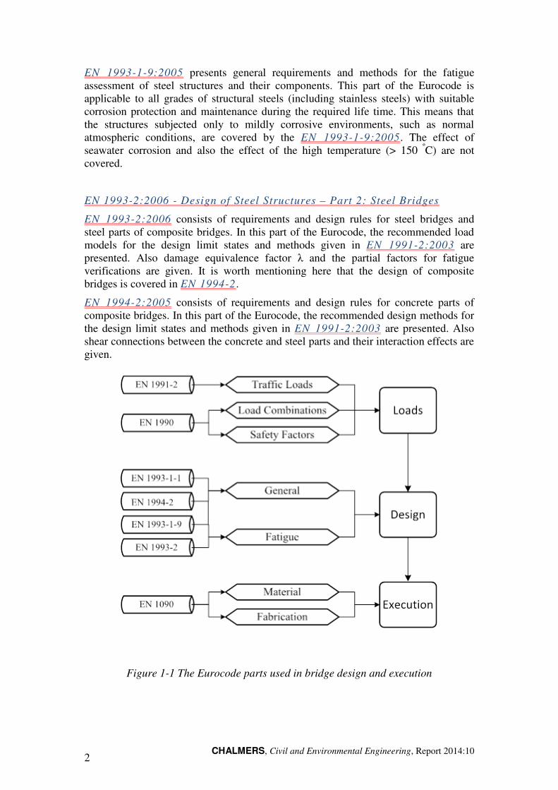
The different parts of the Eurocodes dealing with the design of steel bridges and steel parts of composite bridges are listed in Figure 1-1 and describe below.
EN 1090 - Execution of steel structures
EN 1090 includes the general conditions and requirements for the execution of steel structures. The execution of steel structures is covered to the quality of the construction materials and products that should be used. Special requirements of seismic design are not covered by EN 1090.
EN 1990:2002 – Basis of structural design
The general principles and rules for the design and production works of structures, structural safety, serviceability and durability are presented in EN 1990:2002, which is intended to be used together with the other Eurocode parts. During bridge design stage when calculating the loads on structures, the partial factors to be used for load combinations are presented in this part of the Eurocode.
EN 1991-2:2003 - Actions on structures – Part 2: Traffic loads on bridges
Traffic loads on bridges to be used for different design limit states are defined in EN 1991 in part 2. The code provides imposed loads for different proportions of the various types of standardised vehicles/trains according to the type of bridges and traffics. EN 1991-2:2003 is also intended to be used together with EN 1990 and EN 1991 to EN 1999.
EN 1993-1-9:2005 - Design of Steel Structures – Part 1 – 9: Fatigue
CHALMERS, Civil and Environmental Engineering, Report 2014:10 2
EN 1993-1-9:2005 presents general requirements and methods for the fatigue assessment of steel structures and their components. This part of the Eurocode is applicable to all grades of structural steels (including stainless steels) with suitable corrosion protection and maintenance during the required life time. This means that the structures subjected only to mildly corrosive environments, such as normal atmospheric conditions, are covered by the EN 1993-1-9:2005. The effect of seawater corrosion and also the effect of the high temperature (> 150 ºC) are not covered.
EN 1993-2:2006 - Design of Steel Structures – Part 2: Steel Bridges
EN 1993-2:2006 consists of requirements and design rules for steel bridges and steel parts of composite bridges. In this part of the Eurocode, the recommended load models for the design limit states and methods given in EN 1991-2:2003 are presented. Also damage equivalence factor λ and the partial factors for fatigue verifications are given. It is worth mentioning here that the design of composite bridges is covered in EN 1994-2.
EN 1994-2:2005 consists of requirements and design rules for concrete parts of composite bridges. In this part of the Eurocode, the recommended design methods for the design limit states and methods given in EN 1991-2:2003 are presented. Also shear connections between the concrete and steel parts and their interaction effects are given.
Figure 1-1 The Eurocode parts used in bridge design and execution
CHALMERS, Civil and Environmental Engineering, Report 2014: 3
1.2 Application areas and limitations
The applicability of the fatigue design recommendations and guidelines given in this document is limited by the scopes and limitations of the various relevant parts in the Eurocode.
1.2.1 Material
The range of structural steel grades used in steel bridges is given in Table 3.1 in EN 1993-1-1:2005. The code also recommends that for material properties and geometrical data to be used in design of steel bridges the relevant ENs, ETA or ETA product standard should be complied. Higher structural steel grades (> S700) are however listed in EN 1993-1-12:2007.
1.2.2 Temperature
It is well-known that material properties are dependent on the temperature. The effect of temperature on the fatigue strength of a detail should be checked due to fact that the temperature effect for example with a very low temperature can change the crack growth rate which can in turn change the fatigue strength of structural steels.
With a high temperature, the fatigue strength of structural steel might be reduced because of the increased plastic deformation which can lead to increased fatigue damage accumulation [1]. However, temperatures above 150 ºC are not considered in EN 1993-1-1:2005 when computing the fatigue strength of structural steels. Instead, high temperature above 150 ºC should be considered as the temperature induced damage or additional load in form of temperature following recommendations given in EN 1991-1-1:2005 when computing the reduced fatigue strength.
1.2.3 Corrosion
Fatigue strength of materials can be affected by the environment which can influence both the crack initiation and crack growth phase of fatigue cracks. Corrosion can reduce the fatigue life of a structure by introducing surface flaws which can be considered as local stress raisers that may cause high stress concentrations. Therefore, structural steels should be protected against corrosion.
CHALMERS, Civil and Environmental Engineering, Report 2014:10 4
2 Fatigue load models in Eurocode
Load effects generated by traffic loads on bridges are generally very complex. Not only are the stress ranges generated by these loads of variable amplitudes, but also other parameters that might affect the fatigue performance of bridge details such as the mean stress values and the sequence of loading cycles are rather stochastic.
In order to treat such complex loading situations there is a need to represent the “real” traffic loads in term of one or more equivalent load models. Expressed in term of load effects (i.e. stresses and deformation) the variable amplitude stress ranges generated by real traffic loads on bridges should be represented as one or more equivalent constant amplitude stress ranges, which are easier to treat in a design situation. In doing so, the fatigue damage generated by these equivalent load models should be equivalent to that caused by the real traffic load on bridges. The fatigue load models in EN 1990 and EN 1991-2 were derived on the basis of these principles.
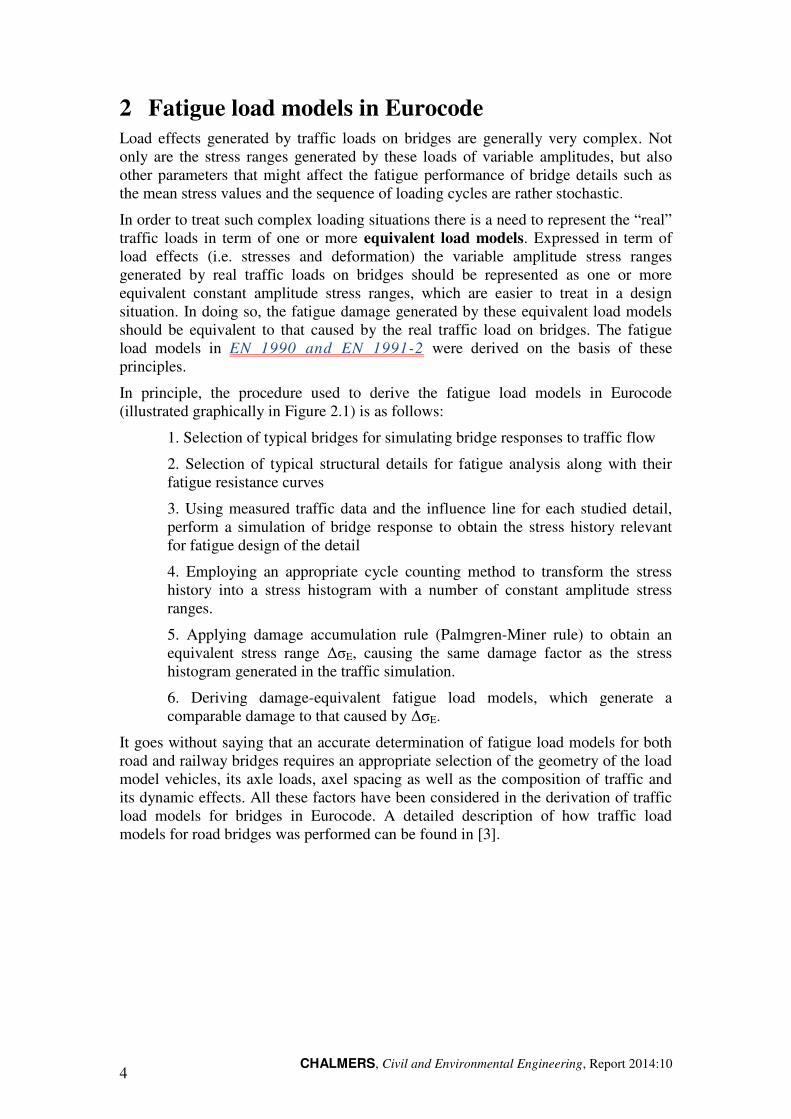
In principle, the procedure used to derive the fatigue load models in Eurocode (illustrated graphically in Figure 2.1) is as follows:
1. Selection of typical bridges for simulating bridge responses to traffic flow
2. Selection of typical structural details for fatigue analysis along with their fatigue resistance curves
3. Using measured traffic data and the influence line for each studied detail, perform a simulation of bridge response to obtain the stress history relevant for fatigue design of the detail
4. Employing an appropriate cycle counting method to transform the stress history into a stress histogram with a number of constant amplitude stress ranges.
5. Applying damage accumulation rule (Palmgren-Miner rule) to obtain an equivalent stress range ∆σE, causing the same damage factor as the stress histogram generated in the traffic simulation.
6. Deriving damage-equivalent fatigue load models, which generate a comparable damage to that caused by ∆σE.
It goes without saying that an accurate determination of fatigue load models for both road and railway bridges requires an appropriate selection of the geometry of the load model vehicles, its axle loads, axel spacing as well as the composition of traffic and its dynamic effects. All these factors have been considered in the derivation of traffic load models for bridges in Eurocode. A detailed description of how traffic load models for road bridges was performed can be found in [3].
CHALMERS, Civil and Environmental Engineering, Report 2014: 5
σ∆
Figure 2-1 The principles for the derivation of fatigue load models in the Eurocode

CHALMERS, Civil and Environmental Engineering, Report 2014:10 6
2.1 Fatigue load models for road bridges
The fatigue load models for road bridges recommended in EN 1991-2:2003 were derived according to the procedure presented in the previous section. In EN 1991-2:2003, there are totally five recommended fatigue load models to reflect the actual load conditions accurately when designing road bridges against fatigue. These fatigue load models have been defined and calibrated based on a wide range of European traffic data measurements in which the traffic measured during the two measurement periods, the years 1977 – 1982 and 1984 – 1988. These measurements recorded on various types of roads and bridges in different European countries [3]. Figure 2-2 shows an example from these traffic measurements presented as percentage of vehicle type.
Figure 2-2 Percentage of the types of vehicles [3]
CHALMERS, Civil and Environmental Engineering, Report 2014: 7
The Auxerre traffic has been chosen as the basis for the derivation of the load models for road bridges in EN 1991-2:2003. The Auxerre traffic displays neither the largest axle loads nor the longest measurement. However, it has the largest frequency of large axle loads which is an essential factor to derive a characteristic design load for fatigue design of bridges. Another reason for choosing the Auxerre traffic as a common “European traffic” is that the extrapolation method used to determine characteristic values needed a sample of uniform traffic, which was provided by this traffic composition.
All in all, five different load models are proposed in EN 1991-2:2003 for road traffic. The choice of appropriate load model depends on the fatigue verification method used in design. In addition, the use of a specific load model might lead to conservative results in a specific case, while another load model might be more appropriate in a specific situation. In the following sections, a more detailed description of each load model is presented and comments are made on the application of these load models when appropriate.
2.1.1 Fatigue load model 1, FLM1
Fatigue load model 1 (FLM 1) is intended to be used to check an “infinite fatigue design” situation, i.e. to check whether the fatigue life of the bridge may be considered infinite. This load model generates a “constant amplitude” stress range which is the algebraic difference between the minimum and maximum stress obtained from positioning the load model in the corresponding tow positions.
FLM 1 is directly derived from the characteristic load model 1 (LM 1) used in the ULS design by multiplying the concentrated axle loads (Qik) by 0.7 and the weight density of the uniformly distributed loads (qik, qrk) by 0.3. Thus, FLM 1 is composed of both concentrated and uniformly distributed loads. Fatigue verification with FLM 1 is performed by comparing the stress range generated by this model to the Constant Amplitude Fatigue limit (CAFL). Therefore fatigue design using FLM 1 will yield a very heavy structure.
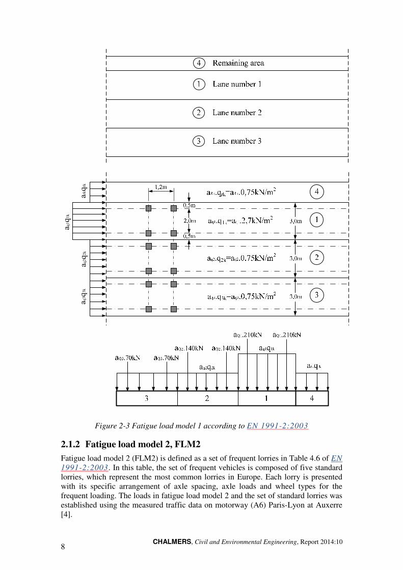
The characteristic LM 1 is composed of double-axle concentrated loads (called the Tandem System) applied in conjunction with a uniformly distributed load (UDL). This load model was developed using measured traffic data on the motorway (A6) Paris-Lyon near Auxerre. The vehicle geometry and the axle loads are specified in EN 1991-2:2003 and reproduced in Figure 2-3 which is recommended for bridges with span length less than 200m. As shown in this figure, the amount of uniformly distributed load applied on bridge lanes including remaining area is the same except for lane number 1, in which a higher fatigue load is recommended. Recommendations for load models for bridges with larger span (≥ 200m) are given in TRVK Bro 11:085.
CHALMERS, Civil and Environmental Engineering, Report 2014:10 8
aq1q
1k
aq2q
2k
arkq
rkaq
3q
3k
Figure 2-3 Fatigue load model 1 according to EN 1991-2:2003
2.1.2 Fatigue load model 2, FLM2
Fatigue load model 2 (FLM2) is defined as a set of frequent lorries in Table 4.6 of EN 1991-2:2003. In this table, the set of frequent vehicles is composed of five standard lorries, which represent the most common lorries in Europe. Each lorry is presented with its specific arrangement of axle spacing, axle loads and wheel types for the frequent loading. The loads in fatigue load model 2 and the set of standard lorries was established using the measured traffic data on motorway (A6) Paris-Lyon at Auxerre [4].
CHALMERS, Civil and Environmental Engineering, Report 2014: 9
Notes on the application of FLM1 and FLM2
• Similar to FLM 1, Fatigue load model 2 is intended to be used of determining
the maximum and minimum stresses when designing for an unlimited fatigue
life. The stress range generated by each lorry should be compared to the
CAFL in the fatigue verification.
• FLM 2 is intended to be used in situations where the presence of more than
one vehicle over the bridge can be neglected. This is the situation for bridge
details with short influence lines, e.g. local bending effects in orthotropic steel
bridge decks. The fatigue verification should therefore be performed for each
vehicle in the traffic set as – dependent on the length of influence line for the
particular detail – an axle load, a bogie axle or an entire vehicle may cause a
loading cycle. Thus for such situations, FLM 2 deliver more accurate results
than FLM 1.
• Fatigue verification applying FLM 1 and FLM 2 is performed by checking that
the stress range (the algebraic difference between the maximum and minimum
stress) for the detail and load effect under consideration does not exceed the
CAFL. This exerts a limitation on the application of these two load models as
for some details, such as welded details loaded in shear, a constant
amplitude fatigue limit is not defined in the code.
2.1.3 Fatigue load model 3, FLM 3
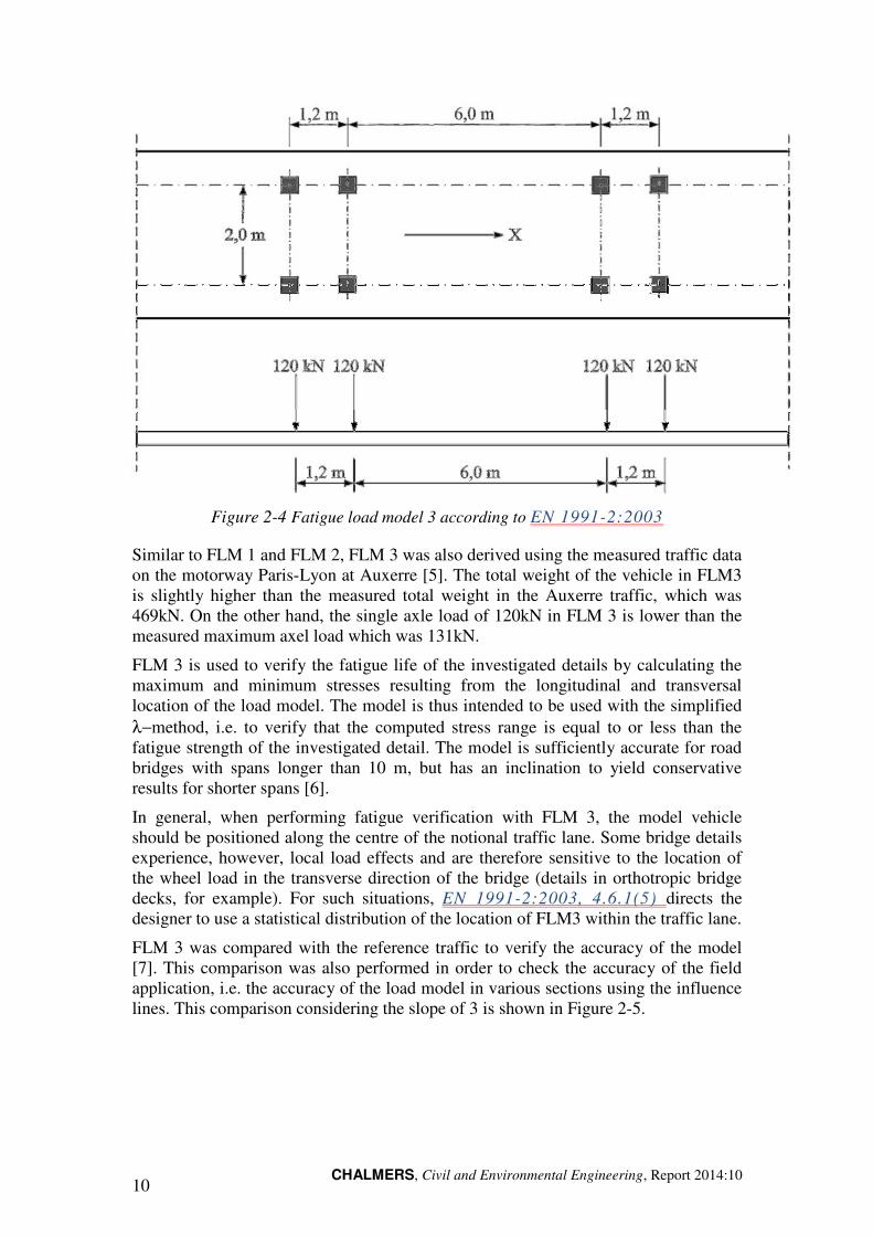
Fatigue Load Model 3 (FLM 3) is composed of a single vehicle with four axles of 120kN each (the total weight of the vehicle is thus 480kN). The vehicle geometry and the axle loads are specified in EN 1991-2:2003 and reproduced in Figure 2-4.
CHALMERS, Civil and Environmental Engineering, Report 2014:10 10
Figure 2-4 Fatigue load model 3 according to EN 1991-2:2003
Similar to FLM 1 and FLM 2, FLM 3 was also derived using the measured traffic data on the motorway Paris-Lyon at Auxerre [5]. The total weight of the vehicle in FLM3 is slightly higher than the measured total weight in the Auxerre traffic, which was 469kN. On the other hand, the single axle load of 120kN in FLM 3 is lower than the measured maximum axel load which was 131kN.
FLM 3 is used to verify the fatigue life of the investigated details by calculating the maximum and minimum stresses resulting from the longitudinal and transversal location of the load model. The model is thus intended to be used with the simplified λ−method, i.e. to verify that the computed stress range is equal to or less than the fatigue strength of the investigated detail. The model is sufficiently accurate for road bridges with spans longer than 10 m, but has an inclination to yield conservative results for shorter spans [6].
In general, when performing fatigue verification with FLM 3, the model vehicle should be positioned along the centre of the notional traffic lane. Some bridge details experience, however, local load effects and are therefore sensitive to the location of the wheel load in the transverse direction of the bridge (details in orthotropic bridge decks, for example). For such situations, EN 1991-2:2003, 4.6.1(5) directs the designer to use a statistical distribution of the location of FLM3 within the traffic lane.
FLM 3 was compared with the reference traffic to verify the accuracy of the model [7]. This comparison was also performed in order to check the accuracy of the field application, i.e. the accuracy of the load model in various sections using the influence lines. This comparison considering the slope of 3 is shown in Figure 2-5.
CHALMERS, Civil and Environmental Engineering, Report 2014: 11
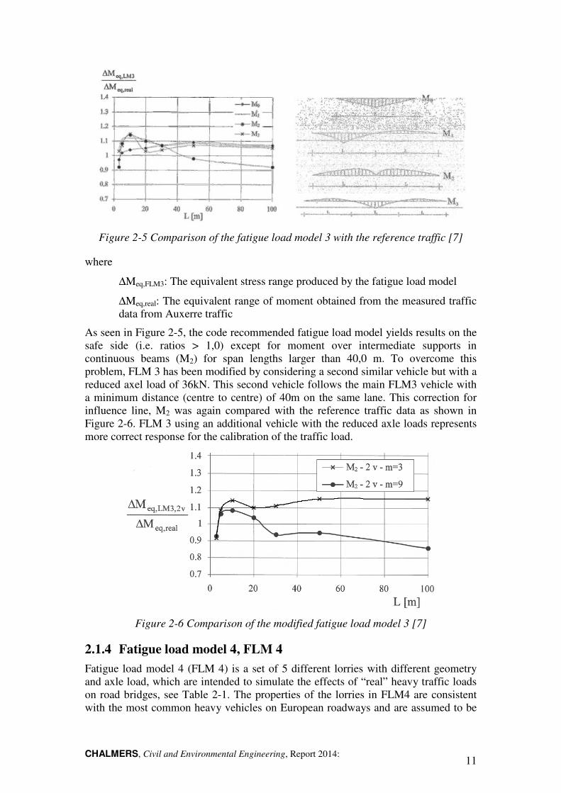
Figure 2-5 Comparison of the fatigue load model 3 with the reference traffic [7]
where
∆Meq,FLM3: The equivalent stress range produced by the fatigue load model
∆Meq,real: The equivalent range of moment obtained from the measured traffic data from Auxerre traffic
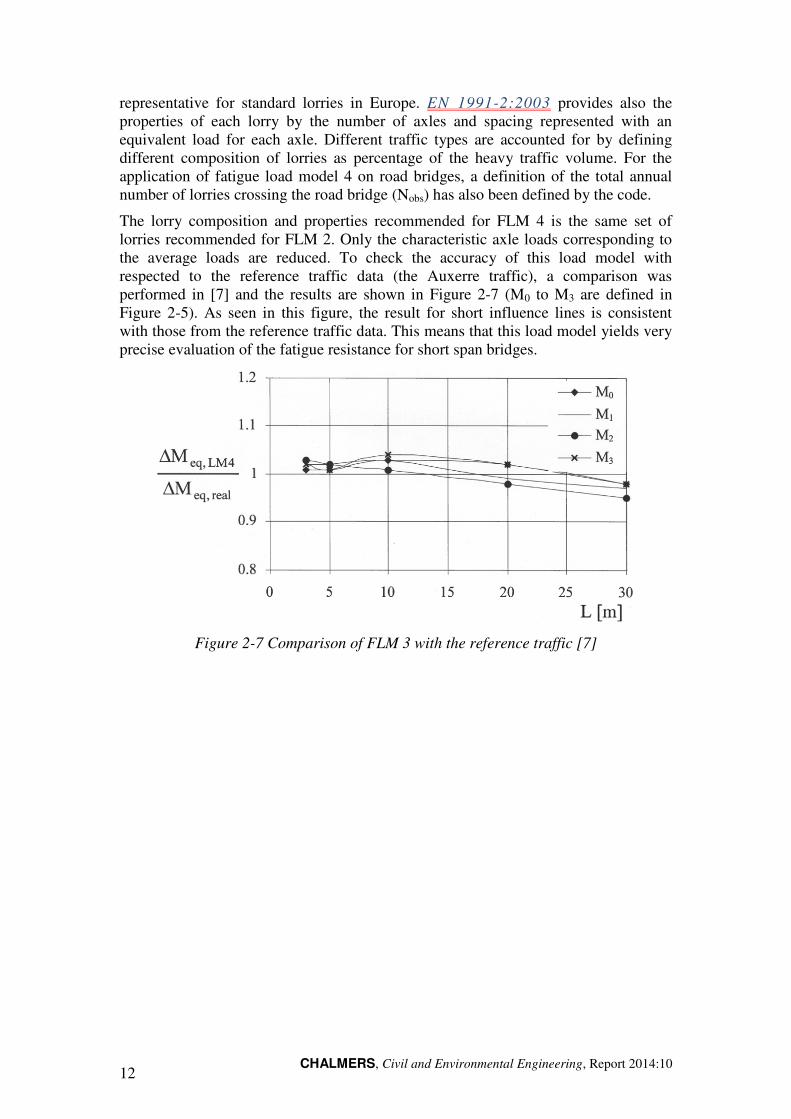
As seen in Figure 2-5, the code recommended fatigue load model yields results on the safe side (i.e. ratios > 1,0) except for moment over intermediate supports in continuous beams (M2) for span lengths larger than 40,0 m. To overcome this problem, FLM 3 has been modified by considering a second similar vehicle but with a reduced axel load of 36kN. This second vehicle follows the main FLM3 vehicle with a minimum distance (centre to centre) of 40m on the same lane. This correction for influence line, M2 was again compared with the reference traffic data as shown in Figure 2-6. FLM 3 using an additional vehicle with the reduced axle loads represents more correct response for the calibration of the traffic load.
Figure 2-6 Comparison of the modified fatigue load model 3 [7]
2.1.4 Fatigue load model 4, FLM 4
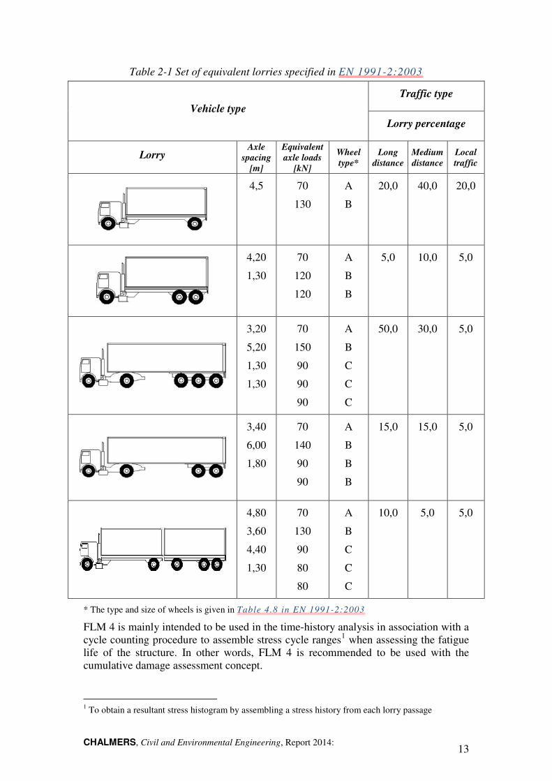
Fatigue load model 4 (FLM 4) is a set of 5 different lorries with different geometry and axle load, which are intended to simulate the effects of “real” heavy traffic loads on road bridges, see Table 2-1. The properties of the lorries in FLM4 are consistent with the most common heavy vehicles on European roadways and are assumed to be
CHALMERS, Civil and Environmental Engineering, Report 2014:10 12
representative for standard lorries in Europe. EN 1991-2:2003 provides also the properties of each lorry by the number of axles and spacing represented with an equivalent load for each axle. Different traffic types are accounted for by defining different composition of lorries as percentage of the heavy traffic volume. For the application of fatigue load model 4 on road bridges, a definition of the total annual number of lorries crossing the road bridge (Nobs) has also been defined by the code.
The lorry composition and properties recommended for FLM 4 is the same set of lorries recommended for FLM 2. Only the characteristic axle loads corresponding to the average loads are reduced. To check the accuracy of this load model with respected to the reference traffic data (the Auxerre traffic), a comparison was performed in [7] and the results are shown in Figure 2-7 (M0 to M3 are defined in Figure 2-5). As seen in this figure, the result for short influence lines is consistent with those from the reference traffic data. This means that this load model yields very precise evaluation of the fatigue resistance for short span bridges.
Figure 2-7 Comparison of FLM 3 with the reference traffic [7]
CHALMERS, Civil and Environmental Engineering, Report 2014: 13
Table 2-1 Set of equivalent lorries specified in EN 1991-2:2003
Vehicle type Traffic type
Lorry percentage
Lorry Axle
spacing [m]
Equivalent axle loads
[kN]
Wheel type*
Long distance
Medium distance
Local traffic
4,5 70
130
A
B
20,0 40,0 20,0
4,20
1,30
70
120
120
A
B
B
5,0 10,0 5,0
3,20
5,20
1,30
1,30
70
150
90
90
90
A
B
C
C
C
50,0 30,0 5,0
3,40
6,00
1,80
70
140
90
90
A
B
B
B
15,0 15,0 5,0
4,80
3,60
4,40
1,30
70
130
90
80
80
A
B
C
C
C
10,0 5,0 5,0
* The type and size of wheels is given in Table 4.8 in EN 1991-2:2003
FLM 4 is mainly intended to be used in the time-history analysis in association with a cycle counting procedure to assemble stress cycle ranges1 when assessing the fatigue life of the structure. In other words, FLM 4 is recommended to be used with the cumulative damage assessment concept.
1 To obtain a resultant stress histogram by assembling a stress history from each lorry passage
CHALMERS, Civil and Environmental Engineering, Report 2014:10 14
Notes to the use of FLM3 and FLM4
• Since both FLM 3 and FLM 4 are meant to be used for fatigue verification
with finite fatigue life (i.e. for a specific design life), the number of cycles
needs to be specified somehow (observe that this was not needed for FLM 1 &
FLM 2 as they are meant to verify that the fatigue life of the bridge is infinite).
For road bridges, the number of cycles is expressed in EN 1991-2:2003 as a
“traffic category”. Four traffic categories are proposed in EN 1991-2:2003,
each with information about the number of slow lanes and the number of
heavy vehicles – observed or estimated – per year and per slow lane, Nobs.
• With slow lane it is meant traffic lanes used predominantly by heavy vehicles
- With heavy vehicles it is meant lorries with a gross weight higher than
100kN
- Nobs for each traffic category are a nationally determined parameter. The
indicative figures for Nobs in EN 1991-2:2003, 4.6.1(3) for different
traffic categories are replaced in TRVK Bro 11:085 by the values given
in B.3.2.1.3 which is reproduced in the Table below (observe that the
values in the Table below should be doubled for road bridges with single
lane). Annual average daily traffic, abbreviated AADT (ÅDT in Swedish),
is a mean value that refers to the daily traffic volume of a highway for a
year.
- For AADT bigger than 24000 (Category X in the table), a certain
investigation of the prerequisites for the fatigue design should be
performed.
CHALMERS, Civil and Environmental Engineering, Report 2014: 15
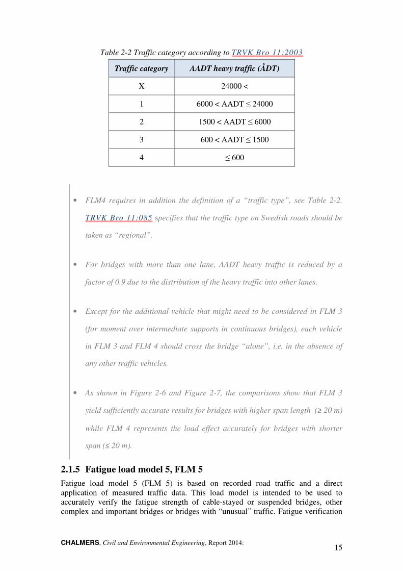
Table 2-2 Traffic category according to TRVK Bro 11:2003
Traffic category AADT heavy traffic (ÅDT)
X 24000 <
1 6000 < AADT ≤ 24000
2 1500 < AADT ≤ 6000
3 600 < AADT ≤ 1500
4 ≤ 600
• FLM4 requires in addition the definition of a “traffic type”, see Table 2-2.
TRVK Bro 11:085 specifies that the traffic type on Swedish roads should be
taken as “regional”.
• For bridges with more than one lane, AADT heavy traffic is reduced by a
factor of 0.9 due to the distribution of the heavy traffic into other lanes.
• Except for the additional vehicle that might need to be considered in FLM 3
(for moment over intermediate supports in continuous bridges), each vehicle
in FLM 3 and FLM 4 should cross the bridge “alone”, i.e. in the absence of
any other traffic vehicles.
• As shown in Figure 2-6 and Figure 2-7, the comparisons show that FLM 3
yield sufficiently accurate results for bridges with higher span length (≥ 20 m)
while FLM 4 represents the load effect accurately for bridges with shorter
span (≤ 20 m).
2.1.5 Fatigue load model 5, FLM 5
Fatigue load model 5 (FLM 5) is based on recorded road traffic and a direct application of measured traffic data. This load model is intended to be used to accurately verify the fatigue strength of cable-stayed or suspended bridges, other complex and important bridges or bridges with “unusual” traffic. Fatigue verification
CHALMERS, Civil and Environmental Engineering, Report 2014:10 16
with FLM 5 requires traffic measurement data, an extrapolation of this data in time and a rather sophisticated statistical analysis. EN 1991-2:2003 provides additional information in this respect in its Annex B.
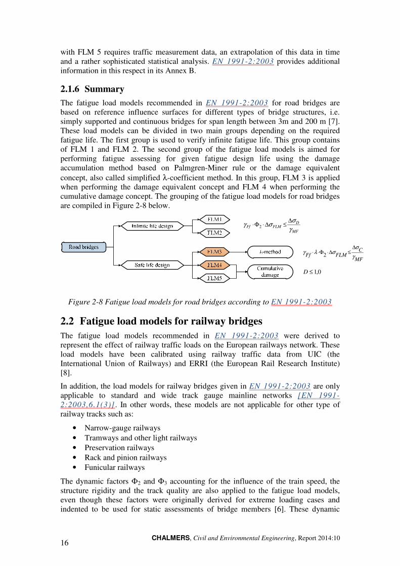
2.1.6 Summary
The fatigue load models recommended in EN 1991-2:2003 for road bridges are based on reference influence surfaces for different types of bridge structures, i.e. simply supported and continuous bridges for span length between 3m and 200 m [7]. These load models can be divided in two main groups depending on the required fatigue life. The first group is used to verify infinite fatigue life. This group contains of FLM 1 and FLM 2. The second group of the fatigue load models is aimed for performing fatigue assessing for given fatigue design life using the damage accumulation method based on Palmgren-Miner rule or the damage equivalent concept, also called simplified λ-coefficient method. In this group, FLM 3 is applied when performing the damage equivalent concept and FLM 4 when performing the cumulative damage concept. The grouping of the fatigue load models for road bridges are compiled in Figure 2-8 below.
MF
DFLMFf
γ
σσγ
∆≤∆⋅Φ⋅ 2
MF
CFLMFf γ
σσλγ
∆≤∆⋅Φ⋅⋅ 2
0,1≤D
Figure 2-8 Fatigue load models for road bridges according to EN 1991-2:2003
2.2 Fatigue load models for railway bridges
The fatigue load models recommended in EN 1991-2:2003 were derived to represent the effect of railway traffic loads on the European railways network. These load models have been calibrated using railway traffic data from UIC (the International Union of Railways) and ERRI (the European Rail Research Institute) [8].
In addition, the load models for railway bridges given in EN 1991-2:2003 are only applicable to standard and wide track gauge mainline networks [EN 1991-2:2003,6.1(3)] . In other words, these models are not applicable for other type of railway tracks such as:
• Narrow-gauge railways • Tramways and other light railways • Preservation railways • Rack and pinion railways • Funicular railways
The dynamic factors Φ2 and Φ3 accounting for the influence of the train speed, the structure rigidity and the track quality are also applied to the fatigue load models, even though these factors were originally derived for extreme loading cases and indented to be used for static assessments of bridge members [6]. These dynamic
CHALMERS, Civil and Environmental Engineering, Report 2014: 17
factors are only valid for train speeds up to 200 km/h. For higher train speeds, special dynamic analysis is required for the fatigue verification in order to more accurately account for additional load effects generated by dynamic effects, such as vibration and resonance.
Unlike the situation for road bridges, fatigue assessment of railway bridges has to be performed according to the “safe life design” principle. Fatigue usually governs the design of railway bridges, and an “infinite life design” approach would result in an extreme and uneconomic design. The λ-coefficient method as well as the cumulative damage method can be used in fatigue verification of railway bridges. Different load models are assigned in EN 1991-2 to be applied in conjunction with each of these methods. These load models are described below.
2.2.1 Fatigue load models for the λλλλ-coefficient method
The fatigue load model to be used for the verification of the fatigue strength of railway bridges when using the damage equivalent concept is derived from load model 71 excluding the ultimate strength design adjustment factor, (α=1.0). In addition to FLM71, load models SW/0 and SW/2 should be used in conjuction with fatigue design of continuous railway bridges with standard and heavy rail traffic respectively. In railway bridges with multiple tracks, fatigue loads should be applied to a maximum of two tracks in the most unfavourable positions for the investigated detail.
2.2.1.1 Fatigue load model 71, FLM 71
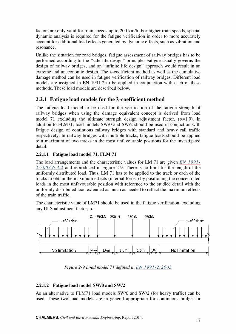
The load arrangements and the characteristic values for LM 71 are given EN 1991-2:2003,6.3.2 and reproduced in Figure 2-9. There is no limit for the length of the uniformly distributed load. Thus, LM 71 has to be applied to the track or each of the tracks to obtain the maximum effects (internal forces) by positioning the concentrated loads in the most unfavourable position with reference to the studied detail with the uniformly distributed load extended as much as needed to reflect the maximum effects of the train traffic.
The characteristic value of LM71 should be used in the fatigue verification, excluding any ULS adjustment factor, α.
Figure 2-9 Load model 71 defined in EN 1991-2:2003
2.2.1.2 Fatigue load model SW/0 and SW/2
As an alternative to FLM71 load models SW/0 and SW/2 (for heavy traffic) can be used. These two load models are in general appropriate for continuous bridges or
CHALMERS, Civil and Environmental Engineering, Report 2014:10 18
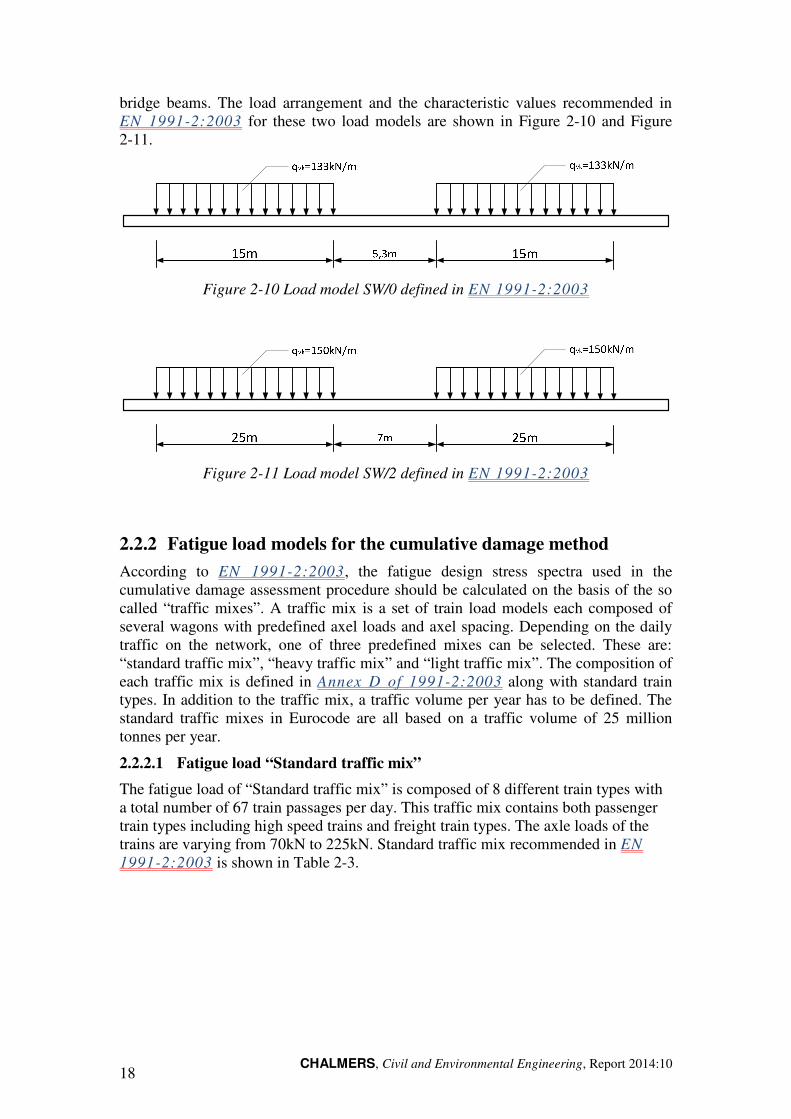
bridge beams. The load arrangement and the characteristic values recommended in EN 1991-2:2003 for these two load models are shown in Figure 2-10 and Figure 2-11.
Figure 2-10 Load model SW/0 defined in EN 1991-2:2003
Figure 2-11 Load model SW/2 defined in EN 1991-2:2003
2.2.2 Fatigue load models for the cumulative damage method
According to EN 1991-2:2003, the fatigue design stress spectra used in the cumulative damage assessment procedure should be calculated on the basis of the so called “traffic mixes”. A traffic mix is a set of train load models each composed of several wagons with predefined axel loads and axel spacing. Depending on the daily traffic on the network, one of three predefined mixes can be selected. These are: “standard traffic mix”, “heavy traffic mix” and “light traffic mix”. The composition of each traffic mix is defined in Annex D of 1991-2:2003 along with standard train types. In addition to the traffic mix, a traffic volume per year has to be defined. The standard traffic mixes in Eurocode are all based on a traffic volume of 25 million tonnes per year.
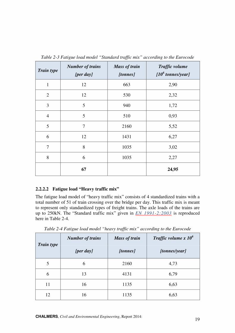
2.2.2.1 Fatigue load “Standard traffic mix”
The fatigue load of “Standard traffic mix” is composed of 8 different train types with a total number of 67 train passages per day. This traffic mix contains both passenger train types including high speed trains and freight train types. The axle loads of the trains are varying from 70kN to 225kN. Standard traffic mix recommended in EN 1991-2:2003 is shown in Table 2-3.
CHALMERS, Civil and Environmental Engineering, Report 2014: 19
Table 2-3 Fatigue load model “Standard traffic mix” according to the Eurocode
Train type Number of trains
[per day]
Mass of train
[tonnes]
Traffic volume
[106 tonnes/year]
1 12 663 2,90
2 12 530 2,32
3 5 940 1,72
4 5 510 0,93
5 7 2160 5,52
6 12 1431 6,27
7 8 1035 3,02
8 6 1035 2,27
67 24,95
2.2.2.2 Fatigue load “Heavy traffic mix”
The fatigue load model of “heavy traffic mix” consists of 4 standardized trains with a total number of 51 of train crossing over the bridge per day. This traffic mix is meant to represent only standardized types of freight trains. The axle loads of the trains are up to 250kN. The “Standard traffic mix” given in EN 1991-2:2003 is reproduced here in Table 2-4.
Table 2-4 Fatigue load model “heavy traffic mix” according to the Eurocode
Train type Number of trains Mass of train Traffic volume x 106
[per day] [tonnes] [tonnes/year]
5 6 2160 4,73
6 13 4131 6,79
11 16 1135 6,63
12 16 1135 6,63
CHALMERS, Civil and Environmental Engineering, Report 2014:10 20
51 24,78
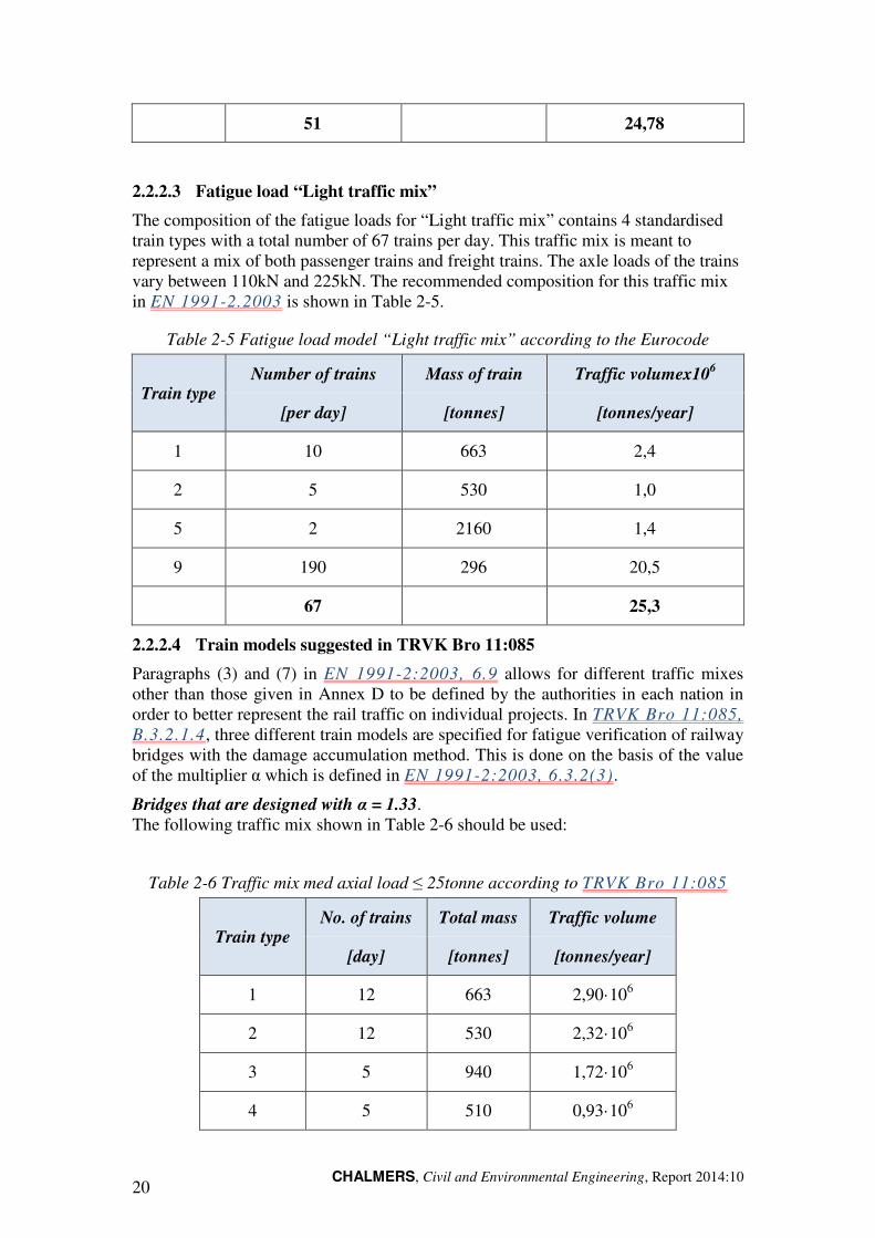
2.2.2.3 Fatigue load “Light traffic mix”
The composition of the fatigue loads for “Light traffic mix” contains 4 standardised train types with a total number of 67 trains per day. This traffic mix is meant to represent a mix of both passenger trains and freight trains. The axle loads of the trains vary between 110kN and 225kN. The recommended composition for this traffic mix in EN 1991-2.2003 is shown in Table 2-5.
Table 2-5 Fatigue load model “Light traffic mix” according to the Eurocode
Train type Number of trains Mass of train Traffic volumex106
[per day] [tonnes] [tonnes/year]
1 10 663 2,4
2 5 530 1,0
5 2 2160 1,4
9 190 296 20,5
67 25,3
2.2.2.4 Train models suggested in TRVK Bro 11:085
Paragraphs (3) and (7) in EN 1991-2:2003, 6.9 allows for different traffic mixes other than those given in Annex D to be defined by the authorities in each nation in order to better represent the rail traffic on individual projects. In TRVK Bro 11:085, B.3.2.1.4, three different train models are specified for fatigue verification of railway bridges with the damage accumulation method. This is done on the basis of the value of the multiplier α which is defined in EN 1991-2:2003, 6.3.2(3).
Bridges that are designed with α = 1.33. The following traffic mix shown in Table 2-6 should be used:
Table 2-6 Traffic mix med axial load ≤ 25tonne according to TRVK Bro 11:085
Train type No. of trains Total mass Traffic volume
[day] [tonnes] [tonnes/year]
1 12 663 2,90·106
2 12 530 2,32·106
3 5 940 1,72·106
4 5 510 0,93·106
CHALMERS, Civil and Environmental Engineering, Report 2014: 21
5 7 2160 5,52·106
6 12 1431 6,27·106
11 7 1135 2,91·106
12 6 1135 2,49·106
66 25,06·106
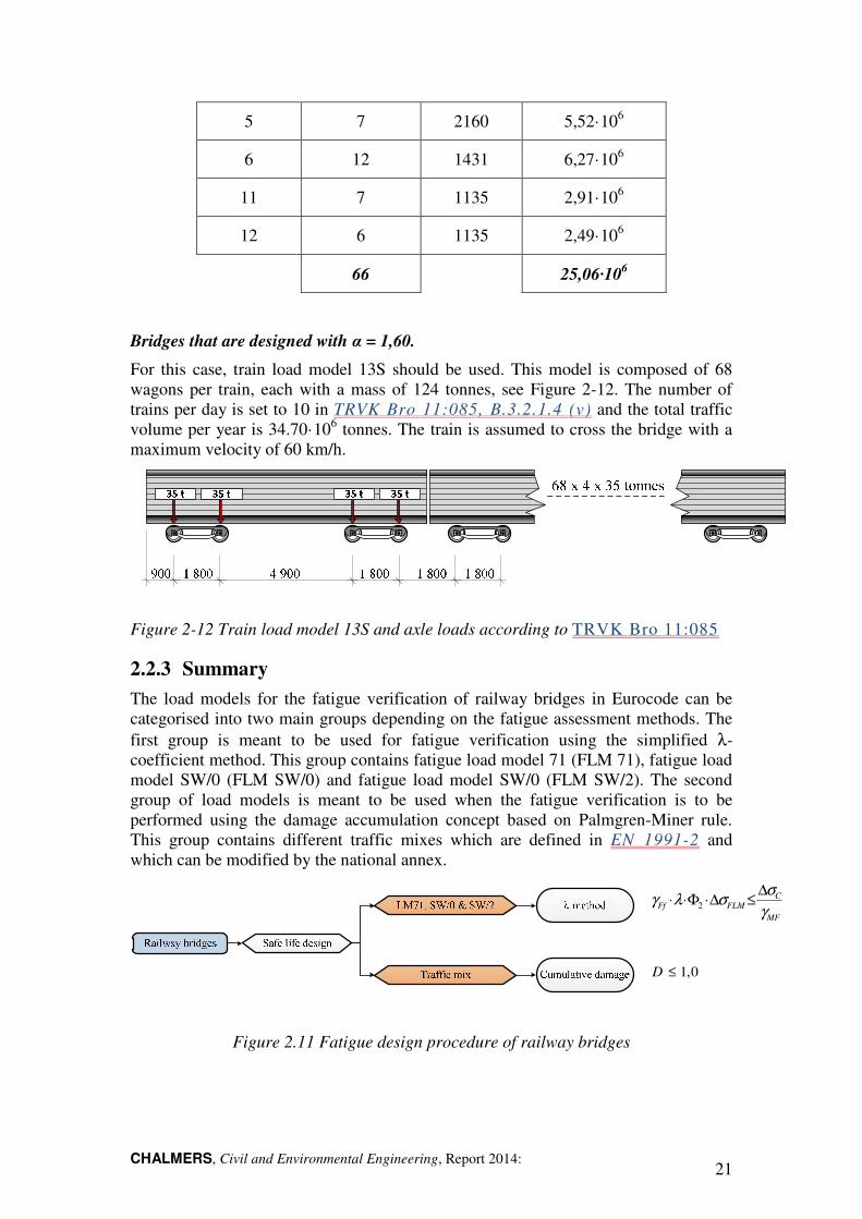
Bridges that are designed with α = 1,60.
For this case, train load model 13S should be used. This model is composed of 68 wagons per train, each with a mass of 124 tonnes, see Figure 2-12. The number of trains per day is set to 10 in TRVK Bro 11:085, B.3.2.1.4 (v) and the total traffic volume per year is 34.70·106 tonnes. The train is assumed to cross the bridge with a maximum velocity of 60 km/h.
Figure 2-12 Train load model 13S and axle loads according to TRVK Bro 11:085
2.2.3 Summary
The load models for the fatigue verification of railway bridges in Eurocode can be categorised into two main groups depending on the fatigue assessment methods. The first group is meant to be used for fatigue verification using the simplified λ-coefficient method. This group contains fatigue load model 71 (FLM 71), fatigue load model SW/0 (FLM SW/0) and fatigue load model SW/0 (FLM SW/2). The second group of load models is meant to be used when the fatigue verification is to be performed using the damage accumulation concept based on Palmgren-Miner rule. This group contains different traffic mixes which are defined in EN 1991-2 and which can be modified by the national annex.
0,1≤D
MF
CFLMFf
γ
σσλγ
∆≤∆⋅Φ⋅⋅ 2
Figure 2.11 Fatigue design procedure of railway bridges

CHALMERS, Civil and Environmental Engineering, Report 2014:10 22

CHALMERS, Civil and Environmental Engineering, Report 2014: 23
3 Fatigue design methods
Eurocode allows for the application of two principal methods for the fatigue design of bridges: The equivalent damage method, also known as the λλλλ-coefficient method, and the more general cumulative damage method. The background and the application of these two methods are presented in this chapter. The two methods are also demonstrated (and to some degree compared) in two worked examples in Chapter 4.
3.1 The concept of Equivalent Stress Range
As was mentioned in the previous Chapter, load effects generated by traffic loads on bridges are generally very complex. The stress ranges generated by these loads are usually of variable amplitudes which are relatively difficult to treat in design situations. There is, therefore, a need to represent the fatigue load effects caused by the “actual” variable amplitude loading in term of an equivalent constant amplitude
load effects.
The treatment of such complex fatigue loading situation is usually treated in the following principle steps:
1. Transformation of the variable amplitude loading into a representative constant amplitude loading. This is usually done by some kind of cyclic
counting method. 2. Using the new set of representative constant amplitude loading to perform the
fatigue design or analysis. This is done either: - directly, by applying the Palmgren-Miner damage accumulation rule, or - by using the equivalent stress range concept.
The rules concerned with the fatigue design of bridges in Eurocode allow for the application of any of these two methods. The simplified λ-method in Eurocode is an adaption of the general equivalent stress range concept corrected by various λ-factors, while a direct application of the Palmgren-Miner rule can alternatively be used. As was discussed in the previous chapter, Specific fatigue load models have been derived and implemented in Eurocode for each of these two methods.
The principles of the damage accumulation rule (Palmgren-Miner) are presented in more details in Section 3.3 of this Chapter. In principle, a structural steel detail subjected to a given stress histogram will fail in fatigue when the damage factor D reaches a specific value. In EN 1993-1-9, the value of the damage factor, D was set to unity. Thus:
∑=∑=i i
i
ii N
nDD Eq. 3-1
with
m
iFf
Mf
C
Ci NN
∆⋅
∆
⋅=σγ
γσ
Eq. 3-2
and ni being the total number of loading cycles in the stress histogram.
CHALMERS, Civil and Environmental Engineering, Report 2014:10 24
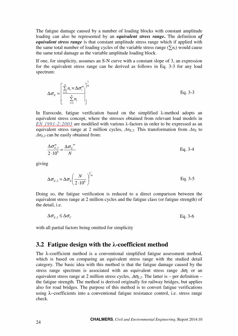
The fatigue damage caused by a number of loading blocks with constant amplitude loading can also be represented by an equivalent stress range. The definition of equivalent stress range is that constant amplitude stress range which if applied with the same total number of loading cycles of the variable stress range (∑ni) would cause the same total damage as the variable amplitude loading block.
If one, for simplicity, assumes an S-N curve with a constant slope of 3, an expression for the equivalent stress range can be derived as follows in Eq. 3-3 for any load spectrum:
m
n
ii
n
i
mii
E
n
n
1
1
1
∑
∑ ∆×=∆
=
=
σσ Eq. 3-3
In Eurocode, fatigue verification based on the simplified λ-method adopts an equivalent stress concept, where the stresses obtained from relevant load models in EN 1991-2:2003 are modified with various λ-factors in order to be expressed as an equivalent stress range at 2 million cycles, ∆σE,2. This transformation from ∆σE to ∆σE,2 can be easily obtained from:
N
m
EmE σσ ∆
=⋅
∆62,
102 Eq. 3-4
giving
m
EE
N1
62, 102
⋅∆=∆ σσ Eq. 3-5
Doing so, the fatigue verification is reduced to a direct comparison between the equivalent stress range at 2 million cycles and the fatigue class (or fatigue strength) of the detail, i.e.
CE σσ ∆≤∆ 2, Eq. 3-6
with all partial factors being omitted for simplicity
3.2 Fatigue design with the λ-coefficient method
The λ-coefficient method is a conventional simplified fatigue assessment method, which is based on comparing an equivalent stress range with the studied detail category. The basic idea with this method is that the fatigue damage caused by the stress range spectrum is associated with an equivalent stress range ∆σE or an equivalent stress range at 2 million stress cycles, ∆σE,2. The latter is – per definition – the fatigue strength. The method is derived originally for railway bridges, but applies also for road bridges. The purpose of this method is to convert fatigue verifications using λ−coefficients into a conventional fatigue resistance control, i.e. stress range check.
CHALMERS, Civil and Environmental Engineering, Report 2014: 25
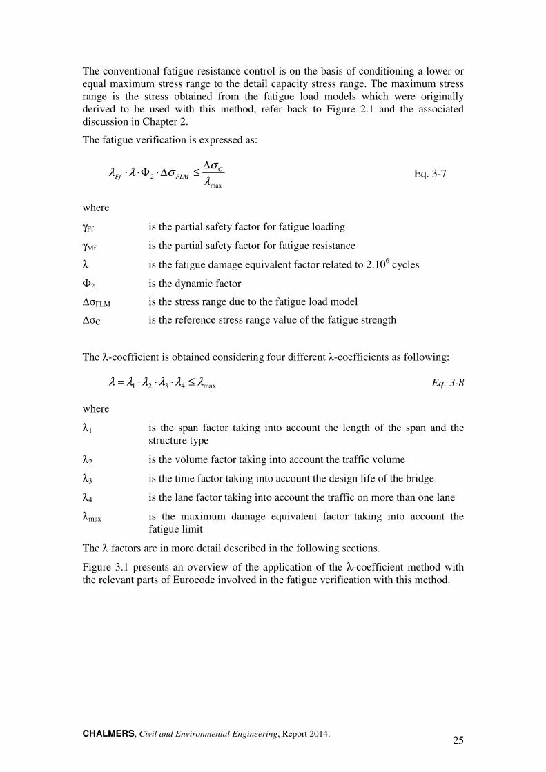
The conventional fatigue resistance control is on the basis of conditioning a lower or equal maximum stress range to the detail capacity stress range. The maximum stress range is the stress obtained from the fatigue load models which were originally derived to be used with this method, refer back to Figure 2.1 and the associated discussion in Chapter 2.
The fatigue verification is expressed as:
max2
λ
σσλλ C
FLMFf
∆≤∆⋅Φ⋅⋅ Eq. 3-7
where
γFf is the partial safety factor for fatigue loading
γMf is the partial safety factor for fatigue resistance
λ is the fatigue damage equivalent factor related to 2.106 cycles
Φ2 is the dynamic factor
∆σFLM is the stress range due to the fatigue load model
∆σC is the reference stress range value of the fatigue strength
The λ-coefficient is obtained considering four different λ-coefficients as following:
max4321 λλλλλλ ≤⋅⋅⋅= Eq. 3-8
where
λ1 is the span factor taking into account the length of the span and the structure type
λ2 is the volume factor taking into account the traffic volume
λ3 is the time factor taking into account the design life of the bridge
λ4 is the lane factor taking into account the traffic on more than one lane
λmax is the maximum damage equivalent factor taking into account the fatigue limit
The λ factors are in more detail described in the following sections.
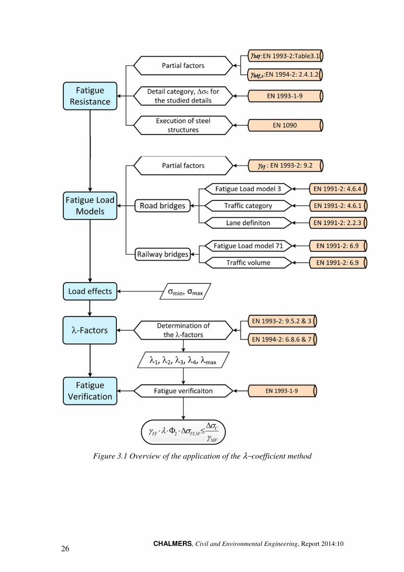
Figure 3.1 presents an overview of the application of the λ-coefficient method with the relevant parts of Eurocode involved in the fatigue verification with this method.
CHALMERS, Civil and Environmental Engineering, Report 2014:10 26
Figure 3.1 Overview of the application of the λ−coefficient method
CHALMERS, Civil and Environmental Engineering, Report 2014: 27
3.2.1 Factor λ1111
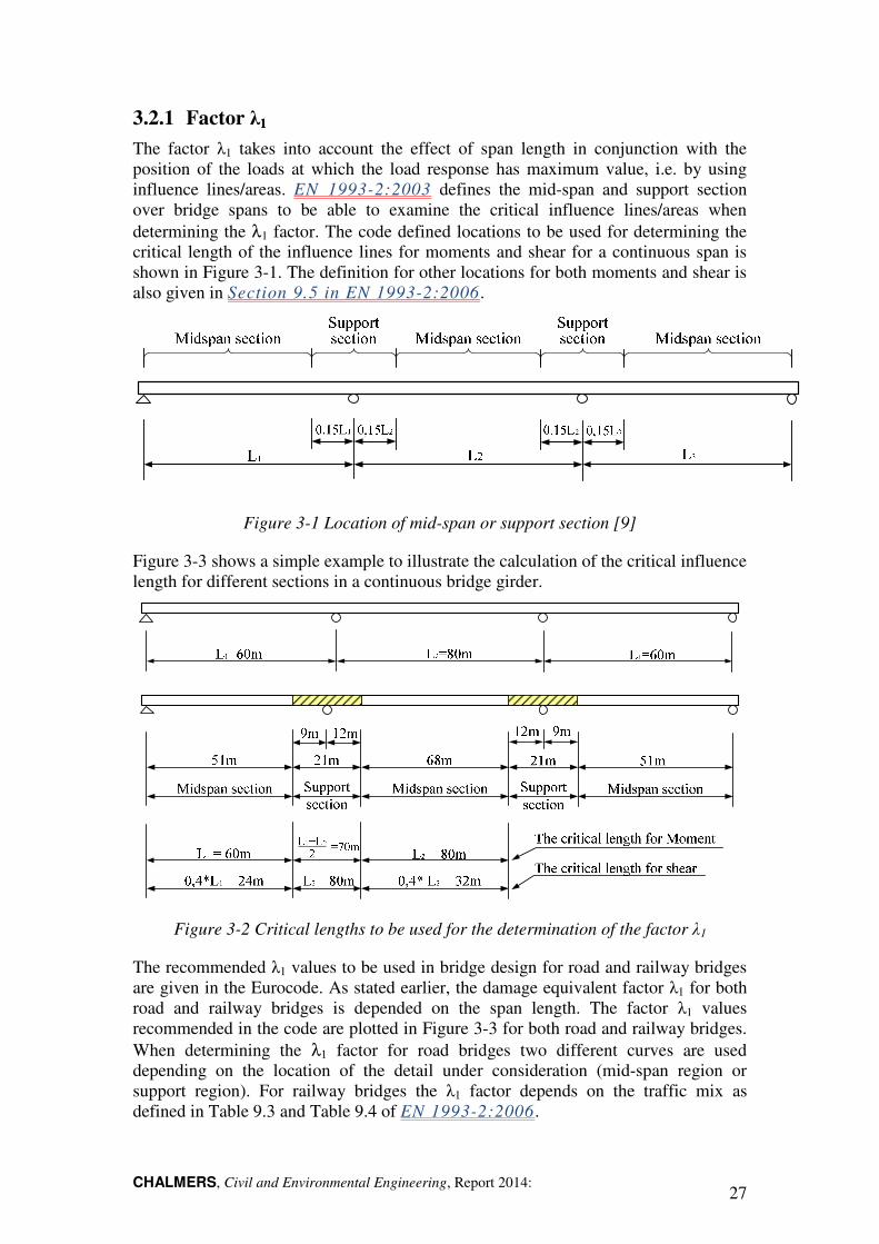
The factor λ1 takes into account the effect of span length in conjunction with the position of the loads at which the load response has maximum value, i.e. by using influence lines/areas. EN 1993-2:2003 defines the mid-span and support section over bridge spans to be able to examine the critical influence lines/areas when determining the λ1 factor. The code defined locations to be used for determining the critical length of the influence lines for moments and shear for a continuous span is shown in Figure 3-1. The definition for other locations for both moments and shear is also given in Section 9.5 in EN 1993-2:2006.
Figure 3-1 Location of mid-span or support section [9]
Figure 3-3 shows a simple example to illustrate the calculation of the critical influence length for different sections in a continuous bridge girder.
Figure 3-2 Critical lengths to be used for the determination of the factor λ1
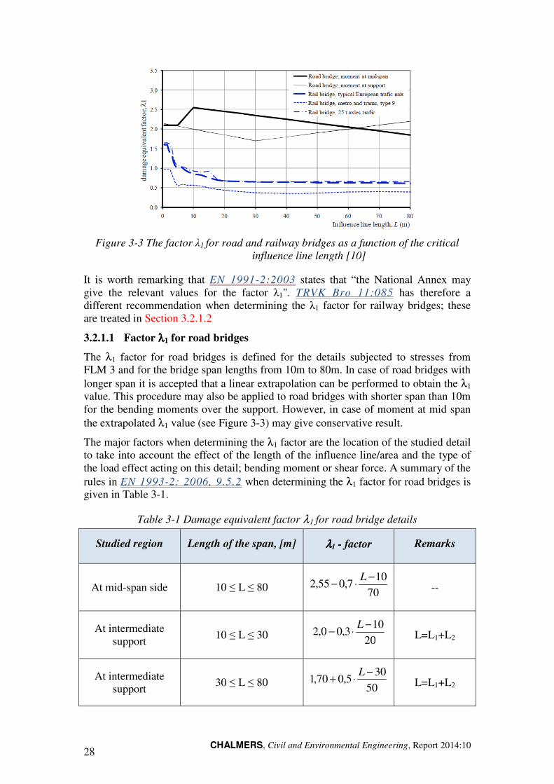
The recommended λ1 values to be used in bridge design for road and railway bridges are given in the Eurocode. As stated earlier, the damage equivalent factor λ1 for both road and railway bridges is depended on the span length. The factor λ1 values recommended in the code are plotted in Figure 3-3 for both road and railway bridges. When determining the λ1 factor for road bridges two different curves are used depending on the location of the detail under consideration (mid-span region or support region). For railway bridges the λ1 factor depends on the traffic mix as defined in Table 9.3 and Table 9.4 of EN 1993-2:2006.
CHALMERS, Civil and Environmental Engineering, Report 2014:10 28
Figure 3-3 The factor λ1 for road and railway bridges as a function of the critical influence line length [10]
It is worth remarking that EN 1991-2:2003 states that “the National Annex may give the relevant values for the factor λ1". TRVK Bro 11:085 has therefore a different recommendation when determining the λ1 factor for railway bridges; these are treated in Section 3.2.1.2
3.2.1.1 Factor λλλλ1111 for road bridges
The λ1 factor for road bridges is defined for the details subjected to stresses from FLM 3 and for the bridge span lengths from 10m to 80m. In case of road bridges with longer span it is accepted that a linear extrapolation can be performed to obtain the λ1 value. This procedure may also be applied to road bridges with shorter span than 10m for the bending moments over the support. However, in case of moment at mid span the extrapolated λ1 value (see Figure 3-3) may give conservative result.
The major factors when determining the λ1 factor are the location of the studied detail to take into account the effect of the length of the influence line/area and the type of the load effect acting on this detail; bending moment or shear force. A summary of the rules in EN 1993-2: 2006, 9.5.2 when determining the λ1 factor for road bridges is given in Table 3-1.
Table 3-1 Damage equivalent factor λ1 for road bridge details
Studied region Length of the span, [m] λλλλ1 - factor Remarks
At mid-span side 10 ≤ L ≤ 80 7010
7,055,2−
⋅−L
--
At intermediate support
10 ≤ L ≤ 30 2010
3,00,2−
⋅−L
L=L1+L2
At intermediate support
30 ≤ L ≤ 80 5030
5,070,1−
⋅+L
L=L1+L2
CHALMERS, Civil and Environmental Engineering, Report 2014: 29
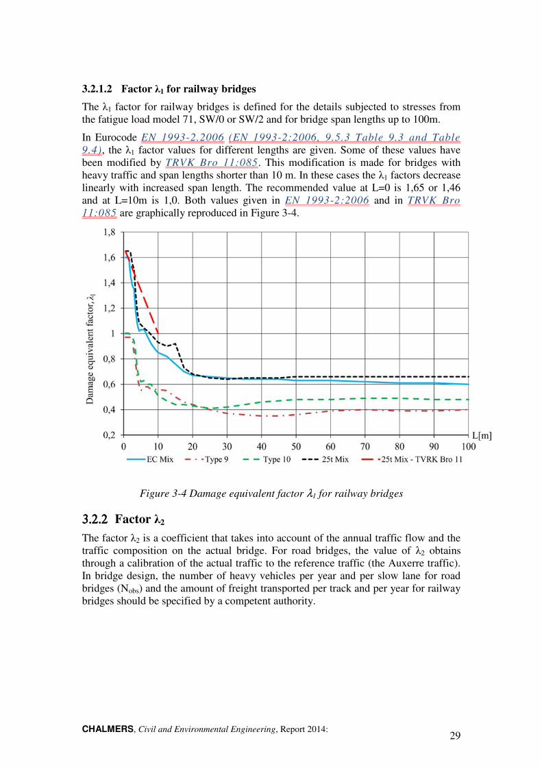
3.2.1.2 Factor λ1 for railway bridges
The λ1 factor for railway bridges is defined for the details subjected to stresses from the fatigue load model 71, SW/0 or SW/2 and for bridge span lengths up to 100m.
In Eurocode EN 1993-2.2006 (EN 1993-2:2006, 9.5.3 Table 9.3 and Table 9.4), the λ1 factor values for different lengths are given. Some of these values have been modified by TRVK Bro 11:085. This modification is made for bridges with heavy traffic and span lengths shorter than 10 m. In these cases the λ1 factors decrease linearly with increased span length. The recommended value at L=0 is 1,65 or 1,46 and at L=10m is 1,0. Both values given in EN 1993-2:2006 and in TRVK Bro 11:085 are graphically reproduced in Figure 3-4.
Figure 3-4 Damage equivalent factor λ1 for railway bridges
3.2.23.2.23.2.23.2.2 Factor λ2
The factor λ2 is a coefficient that takes into account of the annual traffic flow and the traffic composition on the actual bridge. For road bridges, the value of λ2 obtains through a calibration of the actual traffic to the reference traffic (the Auxerre traffic). In bridge design, the number of heavy vehicles per year and per slow lane for road bridges (Nobs) and the amount of freight transported per track and per year for railway bridges should be specified by a competent authority.
CHALMERS, Civil and Environmental Engineering, Report 2014:10 30
3.2.2.1 Factor λ2 for road bridges
According to EN 1993-2:2006, the factor λ2 considering the actual bridge traffic flow and composition should be calculated as following:
m
Obsml
N
N
Q
Q/1
002
⋅=λ Eq. 3-9
where
Qml is the average gross weight (kN) of the lorries in the slow lane
Q0 is the equivalent weight (kN) of the reference traffic
N0 is the annual number of lorries for the reference traffic
NObs is the annual number of lorries in the slow lane
m is the slope of S-N curve; the largest m value in case of bilinear curve
The average gross weight of the lorries in the slow lane can be calculated by the following formula:
m
i
mii
ml n
QnQ
/1
⋅=
∑∑
Eq. 3-10
where
ni is the number of lorries of gross weight Qi in the slow lane
Qi is the gross weight of the lorry “i” in the slow lane
m is the slope of S-N curve; the largest m value in case of bilinear curve
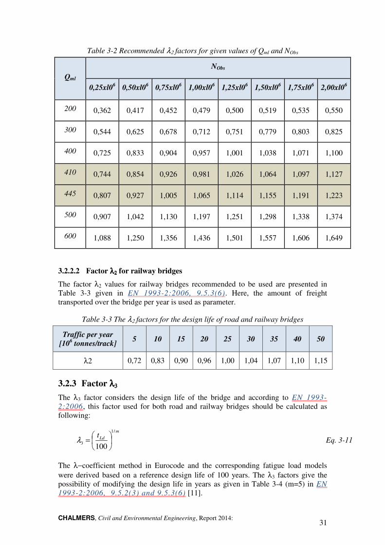
As stated earlier EN 1993-2:2006 is using the Auxerre traffic as the reference traffic data and recommends therefore using N0=0.5x10⁶ and Q0=480kN when calculating the λ2 factor (for this specific case the factor λ2 is equal to 1.0). Based on these two reference values, the factor λ2 for any Qml and NObs can be obtained from Table 9.1 of EN 1993-2:2006, which is reproduced in Table 3-2 (m=5). TRVK Bro 11:085 recommends using Qm1=410kN for regional traffic and Qm1=445kN for long distance traffic. The λ2 factors for these recommended values are also added in Table 3-2 below.
CHALMERS, Civil and Environmental Engineering, Report 2014: 31
Table 3-2 Recommended λ2 factors for given values of Qml and NObs
Qml NObs
0,25xl06 0,50xl06 0,75xl06 1,00xl06 1,25xl06 1,50xl06 1,75xl06 2,00xl06
200 0,362 0,417 0,452 0,479 0,500 0,519 0,535 0,550
300 0,544 0,625 0,678 0,712 0,751 0,779 0,803 0,825
400 0,725 0,833 0,904 0,957 1,001 1,038 1,071 1,100
410 0,744 0,854 0,926 0,981 1,026 1,064 1,097 1,127
445 0,807 0,927 1,005 1,065 1,114 1,155 1,191 1,223
500 0,907 1,042 1,130 1,197 1,251 1,298 1,338 1,374
600 1,088 1,250 1,356 1,436 1,501 1,557 1,606 1,649
3.2.2.2 Factor λλλλ2222 for railway bridges
The factor λ2 values for railway bridges recommended to be used are presented in Table 3-3 given in EN 1993-2:2006, 9.5.3(6). Here, the amount of freight transported over the bridge per year is used as parameter.
Table 3-3 The λ2 factors for the design life of road and railway bridges
Traffic per year [106 tonnes/track] 5 10 15 20 25 30 35 40 50
λ2 0,72 0,83 0,90 0,96 1,00 1,04 1,07 1,10 1,15
3.2.3 Factor λλλλ3333
The λ3 factor considers the design life of the bridge and according to EN 1993-2:2006, this factor used for both road and railway bridges should be calculated as following:
m
Ldt/1
3 100
=λ Eq. 3-11
The λ−coefficient method in Eurocode and the corresponding fatigue load models were derived based on a reference design life of 100 years. The λ3 factors give the possibility of modifying the design life in years as given in Table 3-4 (m=5) in EN 1993-2:2006, 9.5.2(3) and 9.5.3(6) [11].
CHALMERS, Civil and Environmental Engineering, Report 2014:10 32
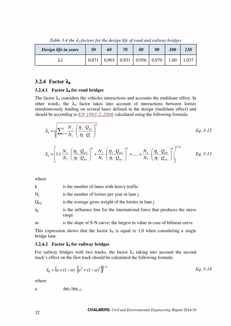
Table 3-4 the λ3 factors for the design life of road and railway bridges
Design life in years 50 60 70 80 90 100 120
λ3 0,871 0,903 0,931 0,956 0,979 1,00 1,037
3.2.4 Factor λλλλ4444
3.2.4.1 Factor λλλλ4444 for road bridges
The factor λ4 considers the vehicles interactions and accounts the multilane effect. In other words, the λ4 factor takes into account of interactions between lorries simultaneously loading on several lanes defined in the design (multilane effect) and should be according to EN 1993-2:2006 calculated using the following formula:
mk
j
m
mjjj
Q
Q
N
N∑ =
⋅
⋅⋅=
1111
4η
ηλ
Eq. 3-12
mm
m
mkkk
m
m
m
m
m
m
Q
Q
N
N
Q
Q
N
N
Q
Q
N
N/1
11111
23
1
3
11
22
1
24 .....1
⋅
⋅⋅++
⋅
⋅⋅+
⋅
⋅⋅+=
η
η
η
η
η
ηλ
Eq. 3-13
where
k is the number of lanes with heavy traffic
Nj is the number of lorries per year in lane j
Qmj is the average gross weight of the lorries in lane j
ηj is the influence line for the international force that produces the stress range
m is the slope of S-N curve; the largest m value in case of bilinear curve
This expression shows that the factor λ4 is equal to 1,0 when considering a single bridge lane.
3.2.4.2 Factor λλλλ4 for railway bridges
For railway bridges with two tracks, the factor λ4 taking into account the second track’s effect on the first track should be calculated the following formula:
[ ]( ) 5/1554 )1()1( aann −+⋅−+=λ
Eq. 3-14
where
a ∆σ1/∆σ1+2
CHALMERS, Civil and Environmental Engineering, Report 2014: 33
∆σ1 is the stress range at the section in interest produced by FLM 71 on the first track
∆σ1+2 is the stress range at the same section produced by FLM 71 on both tracks
n is the percentage of traffic
As seen in this expression, the stress range obtained from the first track will be divided by the stress range which is obtained by adding the stress from both tracks. This means that the factor λ4 will always be smaller than 1,0. This is the major difference between the factor λ4 for railway bridges and the factor λ4 for road bridges.
3.2.5 Factor λλλλmax
The final λ factor is obtained by multiplying the above mentioned individual λ−factors. An upper limit value has also to be considered defined. This is made through the factor λmax which mainly takes into account the fatigue limit of the detail under consideration. The limitation of the damage equivalent factor value for railway bridges is based on the load model which gives an upper bound value while this factor for road bridges is on the same basis as the simulations for the λ1 factor.
3.2.5.1 Factor λλλλmax for road bridges
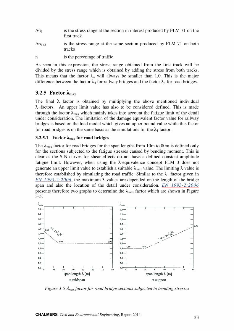
The λmax factor for road bridges for the span lengths from 10m to 80m is defined only for the sections subjected to the fatigue stresses caused by bending moment. This is clear as the S-N curves for shear effects do not have a defined constant amplitude fatigue limit. However, when using the λ-equivalence concept FLM 3 does not generate an upper limit value to establish a suitable λmax value. The limiting λ value is therefore established by simulating the road traffic. Similar to the λ1 factor given in EN 1993-2:2006, the maximum λ values are depended on the length of the bridge span and also the location of the detail under consideration. EN 1993-2:2006 presents therefore two graphs to determine the λmax factor which are shown in Figure 3-5.
Figure 3-5 λmax factor for road bridge sections subjected to bending stresses
CHALMERS, Civil and Environmental Engineering, Report 2014:10 34
3.2.5.2 Factor λλλλmax for railway bridges
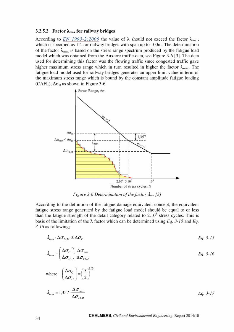
According to EN 1993-2:2006 the value of λ should not exceed the factor λmax, which is specified as 1.4 for railway bridges with span up to 100m. The determination of the factor λmax is based on the stress range spectrum produced by the fatigue load model which was obtained from the Auxerre traffic data, see Figure 3-6 [3]. The data used for determining this factor was the flowing traffic since congested traffic gave higher maximum stress range which in turn resulted in higher the factor λmax. The fatigue load model used for railway bridges generates an upper limit value in term of the maximum stress range which is bound by the constant amplitude fatigue loading (CAFL), ∆σD as shown in Figure 3-6.
Figure 3-6 Determination of the factor λmax [3]
According to the definition of the fatigue damage equivalent concept, the equivalent fatigue stress range generated by the fatigue load model should be equal to or less than the fatigue strength of the detail category related to 2.106 stress cycles. This is basis of the limitation of the λ factor which can be determined using Eq. 3-15 and Eq. 3-16 as following;
CFLM σσλ ∆≤∆⋅max Eq. 3-15
FLMD
C
σ
σ
σ
σλ
∆
∆⋅
∆
∆= max
max
Eq. 3-16
where 3/1
25
=
∆
∆
D
C
σ
σ
FLMσ
σλ
∆
∆⋅= max
max 357,1
Eq. 3-17
CHALMERS, Civil and Environmental Engineering, Report 2014: 35
3.3 Fatigue design with the Damage Accumulation Method
Load effects generated by traffic loads on bridges are generally very complex. Not only are the stress ranges generated by these loads of variable amplitudes, but also other parameters that might affect the fatigue performance of bridge details such as the mean stress values and the sequence of loading cycles are rather stochastic.
In order to treat such complex loading situations there is a need to represent the fatigue load effects caused by the “actual” variable amplitude loading in term of equivalent constant amplitude loading. In other words, a complex loading situation such as the one shown in Figure 3-8 should be represented as one or more equivalent constant amplitude loads, so that the latter will cause equivalent fatigue damage as the real loading history. Two steps are needed:
Transformation of the variable amplitude loading into a representative constant amplitude loading, this is usually done by some kind of cyclic counting method.
Using the new set of representative constant amplitude loading to perform the fatigue design or analysis, this is done either:
- directly, by applying the Palmgren-Miner damage accumulation rule, or - by using the equivalent stress range concept
The rules concerned with the fatigue design of bridges in Eurocode allow for the application of any of these two methods. The simplified λ-method in Eurocode is an adaption of the general equivalent stress range concept corrected by various λ-factors, while a direct application of the Palmgren-Miner rule can alternatively be used for both railway and road bridges.
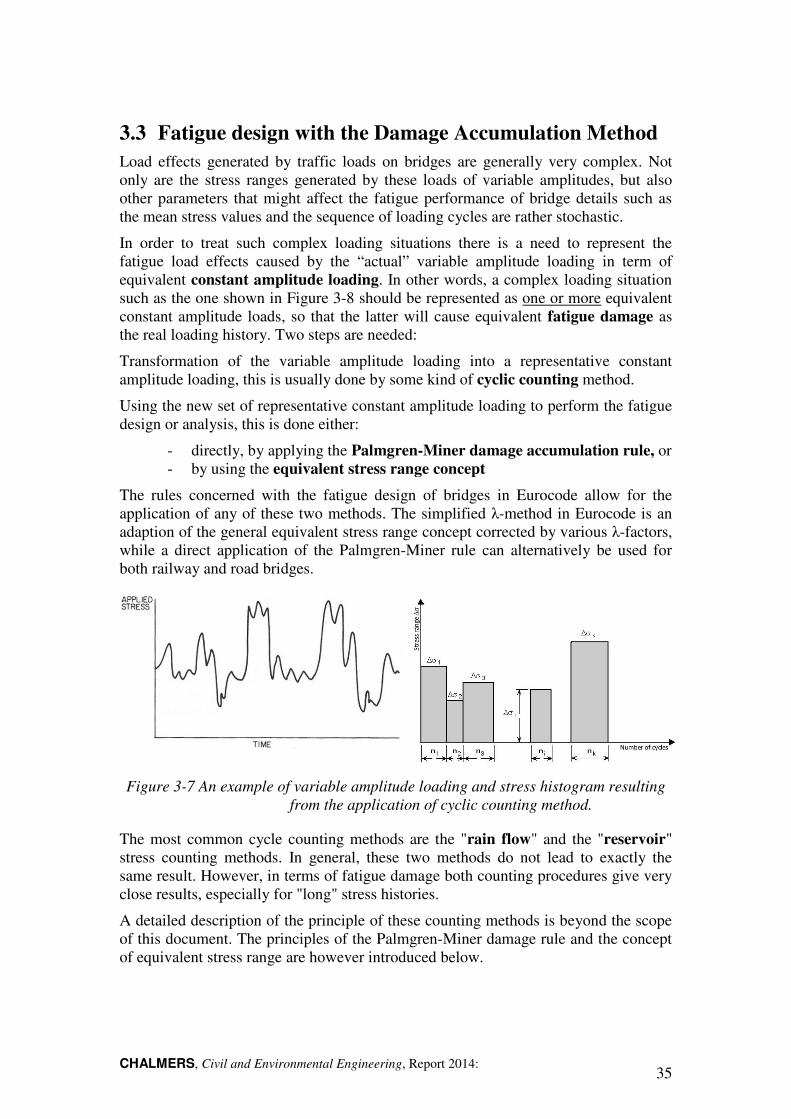
Figure 3-7 An example of variable amplitude loading and stress histogram resulting from the application of cyclic counting method.
The most common cycle counting methods are the "rain flow" and the "reservoir" stress counting methods. In general, these two methods do not lead to exactly the same result. However, in terms of fatigue damage both counting procedures give very close results, especially for "long" stress histories.
A detailed description of the principle of these counting methods is beyond the scope of this document. The principles of the Palmgren-Miner damage rule and the concept of equivalent stress range are however introduced below.
CHALMERS, Civil and Environmental Engineering, Report 2014:10 36
3.4 Palmgren-Miner damage accumulation
As known, an S-N curve represents the relation between the stress range ∆σ (or ∆τ) in a specific detail and the total number of cycles to failure, N. In other words, a specific detail with a certain fatigue strength (represented by an S-N curve) will fail after N cycles of a stress range ∆σ. At failure, the fatigue life is consumed and the total fatigue damage in the detail would then be 100%, or D = 1,0. If the same detail is now loaded with a number of stress cycles n < N at the same stress range, the fatigue damage accumulated in the detail would then be:
N
nD = Eq. 3-18
giving:
D = 1,0 when n = N
D < 1,0 when n < N
With this in mind, if the detail is subjected to a number i of loading blocks each with a constant amplitude stresses ∆σi which is repeated ni number of times, then the total fatigue damage accumulated in the detail would be the sum of the damage caused by the individual loading blocks:
∑=∑=i i
i
ii N
nDD Eq. 3-19
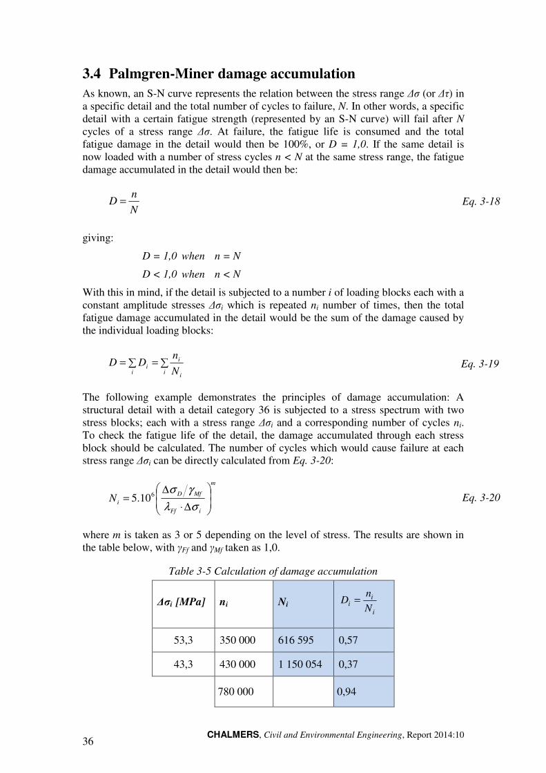
The following example demonstrates the principles of damage accumulation: A structural detail with a detail category 36 is subjected to a stress spectrum with two stress blocks; each with a stress range ∆σi and a corresponding number of cycles ni. To check the fatigue life of the detail, the damage accumulated through each stress block should be calculated. The number of cycles which would cause failure at each stress range ∆σi can be directly calculated from Eq. 3-20:
m
iFf
MfDiN
∆⋅
∆=
σλ
γσ610.5
Eq. 3-20
where m is taken as 3 or 5 depending on the level of stress. The results are shown in the table below, with γFf and γMf taken as 1,0.
Table 3-5 Calculation of damage accumulation
∆σi [MPa] ni Ni i
ii N
nD =
53,3 350 000 616 595 0,57
43,3 430 000 1 150 054 0,37
780 000 0,94

CHALMERS, Civil and Environmental Engineering, Report 2014: 37
3.5 The application of Equivalent Stress Range
As stated earlier, the fatigue damage caused by a number of loading blocks with constant amplitude loading can be represented by an equivalent stress range which is
defined as constant amplitude stress range which if applied with the same total number of loading cycles of the variable stress range would cause the same total damage as the variable amplitude loading block.
If one, for simplicity, assumes an S-N curve with a constant slope of 3, an expression for the equivalent stress range can be derived as follows for any load spectrum:
The damage caused by each loading block in the loading spectrum is
i
ii N
nD =
Eq. 3-21
and the total damage is:
∑=i
iDD
Eq. 3-22
For a design curve with a constant slope m=3 the total number of cycles to cause failure Ni at a specific stress range ∆σi can be expressed as (partial factors are omitted for clarity):
3
6105
∆⋅
∆
⋅⋅=iFf
Mf
D
iNσγ
γσ
Eq. 3-23
Eq. 3-23 can also be writes as (∆σC is the stress at 2 million stress cycles):
3
6102
∆⋅
∆
⋅⋅=iFf
Mf
C
iNσγ
γσ
Eq. 3-24
Thus,
361
3
105 D
n
iiin
Dσ
σ
∆⋅⋅
∑ ∆⋅= = Eq. 3-25
Per definition, the equivalent stress range ∆σE will cause the same damage D after the same total number of cycles, i.e.
∑⋅∆⋅⋅
∆=
∑=
=
=n
ii
D
E
n
ii
E nN
nD
136
31
105 σ
σ Eq. 3-26
Therefore:
CHALMERS, Civil and Environmental Engineering, Report 2014:10 38
31
1
1
3
∑
∑ ∆⋅=∆
=
=n
ii
n
iii
E
n
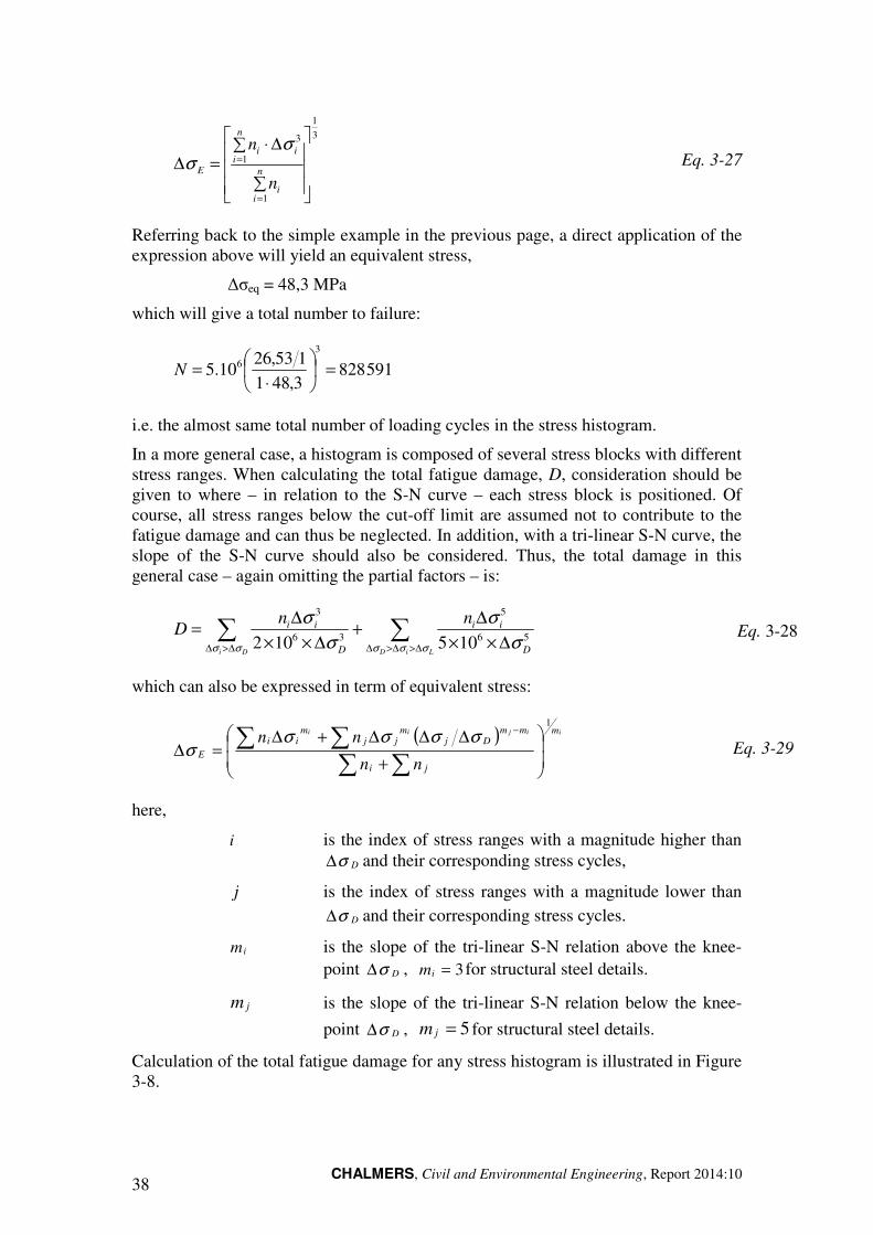
n σσ Eq. 3-27
Referring back to the simple example in the previous page, a direct application of the expression above will yield an equivalent stress,
∆σeq = 48,3 MPa
which will give a total number to failure:
5918283,481153,26
10.53
6 =
⋅=N
i.e. the almost same total number of loading cycles in the stress histogram.
In a more general case, a histogram is composed of several stress blocks with different stress ranges. When calculating the total fatigue damage, D, consideration should be given to where – in relation to the S-N curve – each stress block is positioned. Of course, all stress ranges below the cut-off limit are assumed not to contribute to the fatigue damage and can thus be neglected. In addition, with a tri-linear S-N curve, the slope of the S-N curve should also be considered. Thus, the total damage in this general case – again omitting the partial factors – is:
∑∑∆>∆>∆∆>∆ ∆××
∆+
∆××
∆=
LiDDi D
ii
D
ii nnD
σσσσσ σ
σ
σ
σ56
5
36
3
105102 Eq. 3-28
which can also be expressed in term of equivalent stress:
( ) iijii m
ji
mmDj
mjj
mii
Enn
nn1
+
∆∆∆+∆=∆
∑∑∑∑ −
σσσσσ Eq. 3-29
here,
i is the index of stress ranges with a magnitude higher than Dσ∆ and their corresponding stress cycles,
j is the index of stress ranges with a magnitude lower than
Dσ∆ and their corresponding stress cycles.
im is the slope of the tri-linear S-N relation above the knee-point Dσ∆ , 3=im for structural steel details.
jm is the slope of the tri-linear S-N relation below the knee-
point Dσ∆ , 5=jm for structural steel details.
Calculation of the total fatigue damage for any stress histogram is illustrated in Figure 3-8.
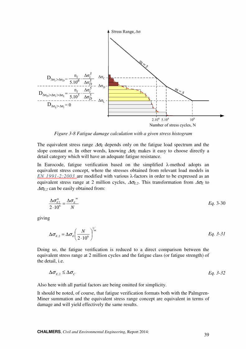
CHALMERS, Civil and Environmental Engineering, Report 2014: 39
Figure 3-8 Fatigue damage calculation with a given stress histogram
The equivalent stress range ∆σE depends only on the fatigue load spectrum and the slope constant m. In other words, knowing ∆σE makes it easy to choose directly a detail category which will have an adequate fatigue resistance.
In Eurocode, fatigue verification based on the simplified λ-method adopts an equivalent stress concept, where the stresses obtained from relevant load models in EN 1991-2:2003 are modified with various λ-factors in order to be expressed as an equivalent stress range at 2 million cycles, ∆σE,2. This transformation from ∆σE to ∆σE,2 can be easily obtained from:
N
m
EmE σσ ∆
=⋅
∆62
102 Eq. 3-30
giving
m
EE
N1
62, 102
⋅∆=∆ σσ Eq. 3-31
Doing so, the fatigue verification is reduced to a direct comparison between the equivalent stress range at 2 million cycles and the fatigue class (or fatigue strength) of the detail, i.e.
CE σσ ∆≤∆ 2, Eq. 3-32
Also here with all partial factors are being omitted for simplicity.
It should be noted, of course, that fatigue verification formats both with the Palmgren-Miner summation and the equivalent stress range concept are equivalent in terms of damage and will yield effectively the same results.
CHALMERS, Civil and Environmental Engineering, Report 2014:10 40
Comment:
- As the fatigue damage factor, D, and the equivalent stress, ∆σE or ∆σE,2
are obtained using the relevant influence lines for load effects and
representative load models, there is no need for any corrections factors,
such as those used in the simplified λ-method.
3.6 The application of the damage accumulation method
Annex A in EN 1993-1-9:2005 gives information on the application of the damage accumulation method in the fatigue design of steel structures. What concerns bridges the use of damage accumulation method is suggested in two cases:
1. When actual traffic data is available. This is covered in Annex B of EN 1991-2:2003 and will not be treated in this document
2. Along with the traffic load models derived for this purpose. These are LM4 for road bridges (EN 1991-2:2003, 4.6.5) and train types 1 to 12 in Annex D of EN 1991-2:2003 of Eurocode
For both road and railway bridges, the traffic load models to be used with the damage accumulation method are intended to reflect the real “heavy” traffic on European road and railway networks. The variation in traffic intensity and vehicle (or train) types on individual bridges is covered by defining different “traffic types” or “traffic mixes” for road and railway traffic respectively. These are also a subject for adaption and modification by the countries through their national annexes.
In the following, the traffic load models proposed in EN 1991-2:2005 for fatigue verification with the cumulative damage concept will be shortly introduced. A summary of the main steps involved in the application of this method is then made. The method is also demonstrated in two worked examples, one for road bridge and one railway bridge.
3.7 Application to road bridges
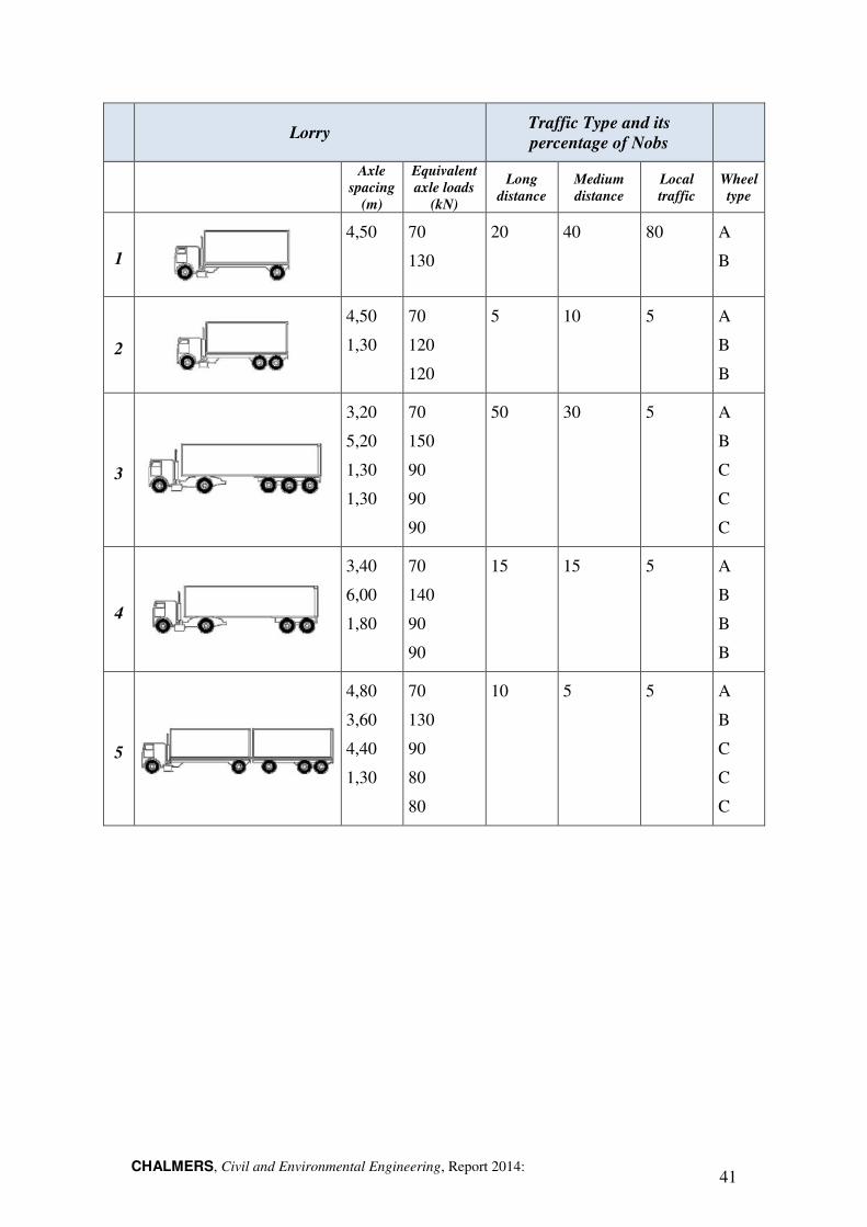
The traffic load model to be used with fatigue verification of road bridges according to the damage accumulation method is load model LM4. This model is composed of 5 standard lorries which are assumed to simulate the effects of real road traffic on the bridge. The definition of each lorry is given by the number of axles, the load on each axle as well as the axle spacing which are reproduced in Table 3-6 and Table 3-7. The number of heavy vehicles, Nobs per year and per slow lane (observed or estimated) applies also for fatigue verification with the damage accumulation method. Indicative figures for Nobs and the recommended values for different traffic categories are given in EN 1991-2:2003 4.6.1(3).
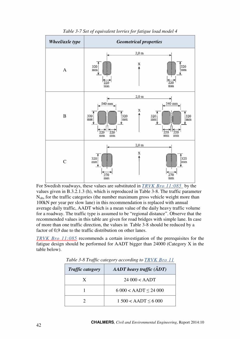
Table 3-6 Set of equivalent lorries for fatigue load model 4
CHALMERS, Civil and Environmental Engineering, Report 2014: 41
Lorry Traffic Type and its percentage of Nobs
Axle
spacing (m)
Equivalent axle loads
(kN)
Long distance
Medium distance
Local traffic
Wheel type
1
4,50 70
130
20 40 80 A
B
2
4,50
1,30
70
120
120
5 10 5 A
B
B
3
3,20
5,20
1,30
1,30
70
150
90
90
90
50 30 5 A
B
C
C
C
4
3,40
6,00
1,80
70
140
90
90
15 15 5 A
B
B
B
5
4,80
3,60
4,40
1,30
70
130
90
80
80
10 5 5 A
B
C
C
C
CHALMERS, Civil and Environmental Engineering, Report 2014:10 42
Table 3-7 Set of equivalent lorries for fatigue load model 4
Wheel/axle type Geometrical properties
A
B
C
For Swedish roadways, these values are substituted in TRVK Bro 11:085 by the values given in B.3.2.1.3 (h), which is reproduced in Table 3-8. The traffic parameter Nobs for the traffic categories (the number maximum gross vehicle weight more than 100kN per year per slow lane) in this recommendation is replaced with annual average daily traffic, AADT which is a mean value of the daily heavy traffic volume for a roadway. The traffic type is assumed to be “regional distance”. Observe that the recommended values in this table are given for road bridges with simple lane. In case of more than one traffic direction, the values in Table 3-8 should be reduced by a factor of 0,9 due to the traffic distribution on other lanes.
TRVK Bro 11:085 recommends a certain investigation of the prerequisites for the fatigue design should be performed for AADT bigger than 24000 (Category X in the table below).
Table 3-8 Traffic category according to TRVK Bro 11
Traffic category AADT heavy traffic (ÅDT)
X 24 000 < AADT
1 6 000 < AADT ≤ 24 000
2 1 500 < AADT ≤ 6 000
CHALMERS, Civil and Environmental Engineering, Report 2014: 43
3 600 < AADT ≤ 1 500
4 AADT ≤ 600
The fatigue verification procedure should be performed – for those details that are determinant for the fatigue performance of the bridge – according to the following steps:
1. Establish the bridge specific data for fatigue verification. Besides the design life of the bridge this includes:
a. the “traffic category” with the associated number of heavy lorries in the slow lane, Nobs [EN 1991-2:2003, 4.6.1(3)] ,
b. the “traffic type” with the associated percentage of lorries, Table 4.7 in EN 1991-2:2003.
2. For the detail in hand, obtain the influence line for relevant load effects (shear or bending stresses).
3. By passing the load model over the influence line, establish the time history response (i.e. stress vs. time, or time step)
4. Construct the stress histogram by mean of a cycle-counting method. For simple cases, such as for simply-supported road bridges, the stress histogram can be easily obtained with hand calculations, see example 4.1 in Section 4.
5. Select an appropriate fatigue category and establish the corresponding S-N curve (∆σC at 2·106 cycles, ∆σD at 5·106 cycles and ∆σL at 100·106 cycles)
6. Use the stress histogram either to:
a. Calculate a total damage
3
6105
∆
∆⋅⋅⋅
⋅=
D
iMfFfii
nD
σ
σγγ if
Mf
DiFf
γ
σσγ
∆≥∆
Eq. 3-33
5
6105
∆
∆⋅⋅⋅
⋅=
D
iMfFfii
nD
σ
σγγ if
Mf
DiFf
Mf
L
γ
σσγ
γ
σ ∆<∆≤
∆ Eq. 3-34
and verify that
0,1≤=∑i
iDD Eq. 3-35
b. Calculate the equivalent stress at 2·106 cycles
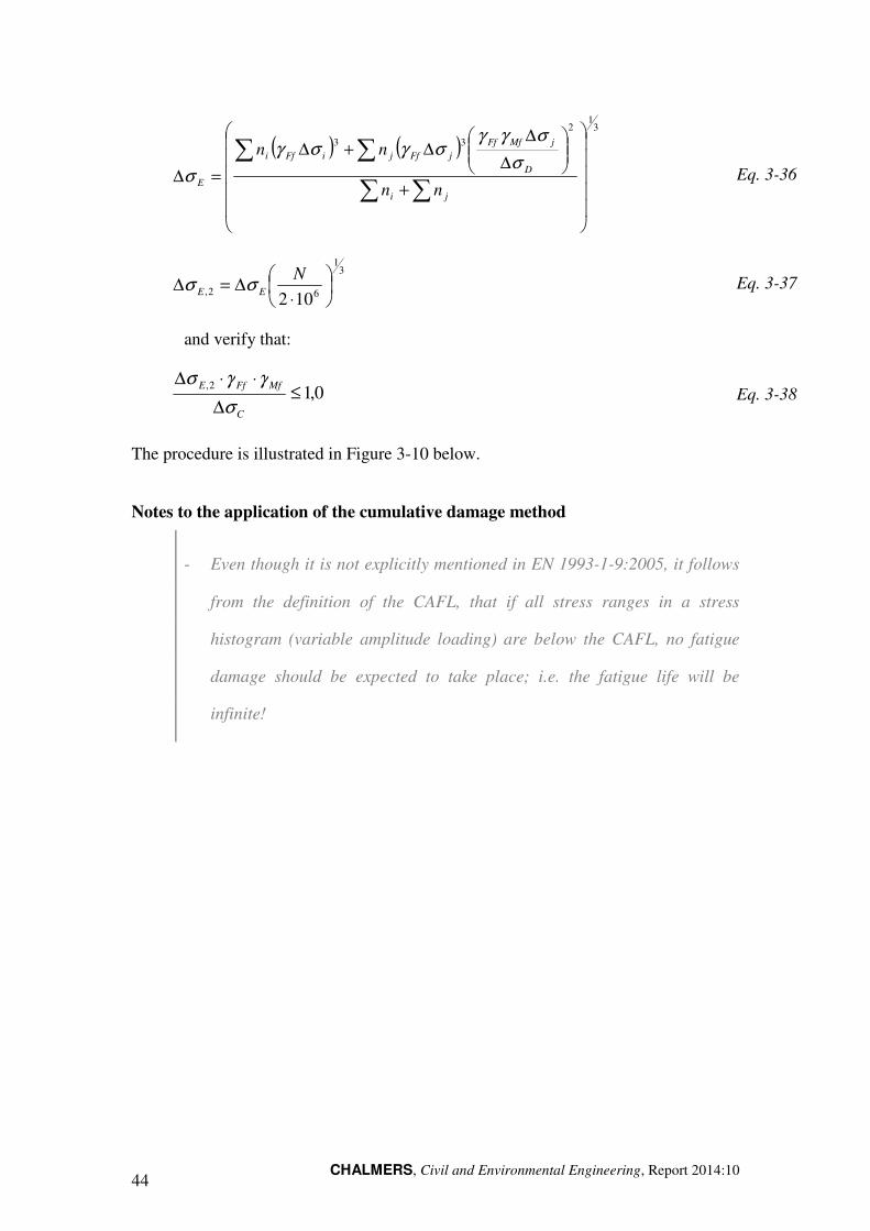
CHALMERS, Civil and Environmental Engineering, Report 2014:10 44
( ) ( )3
12
33
+
∆
∆∆+∆
=∆∑∑
∑∑
ji
D
jMfFfjFfjiFfi
E nn
nnσ
σγγσγσγ
σ
Eq. 3-36
31
62, 102
⋅∆=∆
NEE σσ
Eq. 3-37
and verify that:
0,12,≤
∆
⋅⋅∆
C
MfFfE
σ
γγσ
Eq. 3-38
The procedure is illustrated in Figure 3-10 below.
Notes to the application of the cumulative damage method
- Even though it is not explicitly mentioned in EN 1993-1-9:2005, it follows
from the definition of the CAFL, that if all stress ranges in a stress
histogram (variable amplitude loading) are below the CAFL, no fatigue
damage should be expected to take place; i.e. the fatigue life will be
infinite!
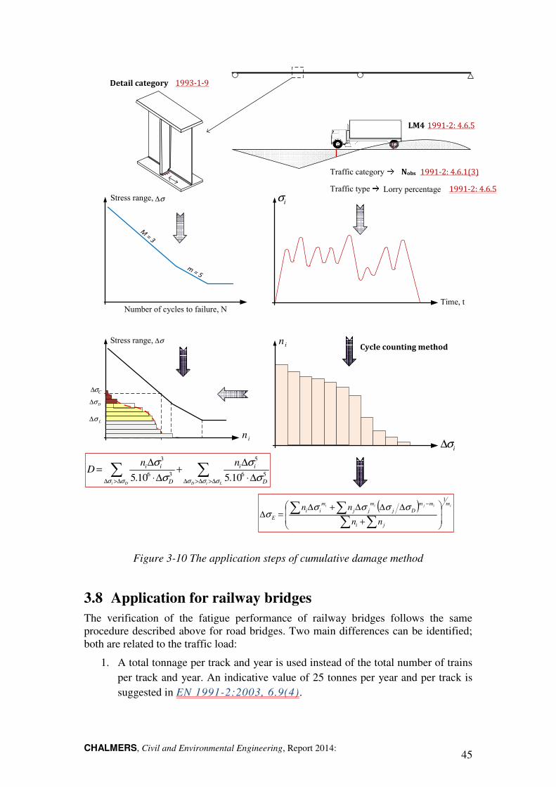
CHALMERS, Civil and Environmental Engineering, Report 2014: 45
iσ∆
in
M = 3
m = 5
σ∆Stress range,
Number of cycles to failure, N
Dσ∆
Cσ∆
Lσ∆
∑∑∆>∆>∆∆>∆ ∆⋅
∆+
∆⋅
∆=
LiDDi D
ii
D
ii nnD
σσσσσ σ
σ
σ
σ56
5
36
3
10.510.5
( ) iijii m
ji
mmDj
mjj
mii
E nn
nn1
+
∆∆∆+∆=∆
∑∑∑∑ −
σσσσσ
1991-2:4.6.5LM4
1993-1-9Detailcategory
1991-2:4.6.1(3)Nobs
Cyclecountingmethod
Traffic category
1991-2:4.6.5Traffic type Lorry percentage
iσ
in
Time, t
σ∆Stress range,
Figure 3-10 The application steps of cumulative damage method
3.8 Application for railway bridges
The verification of the fatigue performance of railway bridges follows the same procedure described above for road bridges. Two main differences can be identified; both are related to the traffic load:
1. A total tonnage per track and year is used instead of the total number of trains per track and year. An indicative value of 25 tonnes per year and per track is suggested in EN 1991-2:2003, 6.9(4).
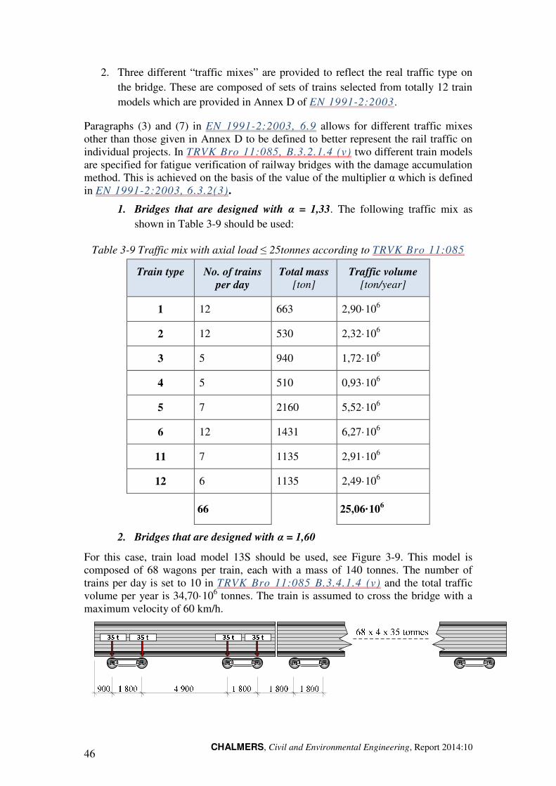
CHALMERS, Civil and Environmental Engineering, Report 2014:10 46
2. Three different “traffic mixes” are provided to reflect the real traffic type on the bridge. These are composed of sets of trains selected from totally 12 train models which are provided in Annex D of EN 1991-2:2003.
Paragraphs (3) and (7) in EN 1991-2:2003, 6.9 allows for different traffic mixes other than those given in Annex D to be defined to better represent the rail traffic on individual projects. In TRVK Bro 11:085, B.3.2.1.4 (v) two different train models are specified for fatigue verification of railway bridges with the damage accumulation method. This is achieved on the basis of the value of the multiplier α which is defined in EN 1991-2:2003, 6.3.2(3).
1. Bridges that are designed with α = 1,33. The following traffic mix as shown in Table 3-9 should be used:
Table 3-9 Traffic mix with axial load ≤ 25tonnes according to TRVK Bro 11:085
Train type No. of trains per day
Total mass [ton]
Traffic volume [ton/year]
1 12 663 2,90·106
2 12 530 2,32·106
3 5 940 1,72·106
4 5 510 0,93·106
5 7 2160 5,52·106
6 12 1431 6,27·106
11 7 1135 2,91·106
12 6 1135 2,49·106
66 25,06·106
2. Bridges that are designed with α = 1,60
For this case, train load model 13S should be used, see Figure 3-9. This model is composed of 68 wagons per train, each with a mass of 140 tonnes. The number of trains per day is set to 10 in TRVK Bro 11:085 B.3.4.1.4 (v) and the total traffic volume per year is 34,70·106 tonnes. The train is assumed to cross the bridge with a maximum velocity of 60 km/h.

CHALMERS, Civil and Environmental Engineering, Report 2014: 47
Figure 3-9 Train load model 13S and axle loads according to TRVK Bro 11:085
Fatigue verification of railway bridges with the damage accumulation method follows the same procedure described in the previous section for road bridges. The application of the traffic mix associated with α = 1,33 is a bit lengthy and might need to be implemented in a computer program. For load model 13S, it is still feasible to perform the calculations in a rather simple way (the axel distances and the axle weights are constant throughout the entire train.
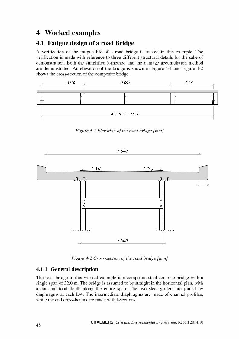
CHALMERS, Civil and Environmental Engineering, Report 2014:10 48
4 Worked examples
4.1 Fatigue design of a road Bridge
A verification of the fatigue life of a road bridge is treated in this example. The verification is made with reference to three different structural details for the sake of demonstration. Both the simplified λ-method and the damage accumulation method are demonstrated. An elevation of the bridge is shown in Figure 4-1 and Figure 4-2 shows the cross-section of the composite bridge.
Figure 4-1 Elevation of the road bridge [mm]
Figure 4-2 Cross-section of the road bridge [mm]
4.1.1 General description
The road bridge in this worked example is a composite steel-concrete bridge with a single span of 32,0 m. The bridge is assumed to be straight in the horizontal plan, with a constant total depth along the entire span. The two steel girders are joined by diaphragms at each L/4. The intermediate diaphragms are made of channel profiles, while the end cross-beams are made with I-sections.
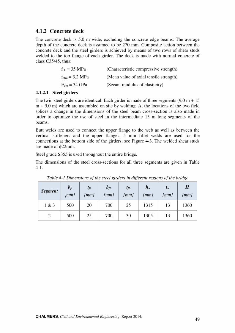
CHALMERS, Civil and Environmental Engineering, Report 2014: 49
4.1.2 Concrete deck
The concrete deck is 5,0 m wide, excluding the concrete edge beams. The average depth of the concrete deck is assumed to be 270 mm. Composite action between the concrete deck and the steel girders is achieved by means of two rows of shear studs welded to the top flange of each girder. The deck is made with normal concrete of class C35/45, thus:
fck = 35 MPa (Characteristic compressive strength)
fctm = 3,2 MPa (Mean value of axial tensile strength)
Ecm = 34 GPa (Secant modulus of elasticity)
4.1.2.1 Steel girders
The twin steel girders are identical. Each girder is made of three segments (9,0 m + 15 m + 9,0 m) which are assembled on site by welding. At the locations of the two field splices a change in the dimensions of the steel beam cross-section is also made in order to optimize the use of steel in the intermediate 15 m long segments of the beams.
Butt welds are used to connect the upper flange to the web as well as between the vertical stiffeners and the upper flanges. 5 mm fillet welds are used for the connections at the bottom side of the girders, see Figure 4-3. The welded shear studs are made of ϕ22mm.
Steel grade S355 is used throughout the entire bridge.
The dimensions of the steel cross-sections for all three segments are given in Table 4-1.
Table 4-1 Dimensions of the steel girders in different regions of the bridge
Segment bft
[mm]
tft
[mm]
bfb
[mm]
tfb
[mm]
hw
[mm]
tw
[mm]
H
[mm]
1 & 3 500 20 700 25 1315 13 1360
2 500 25 700 30 1305 13 1360
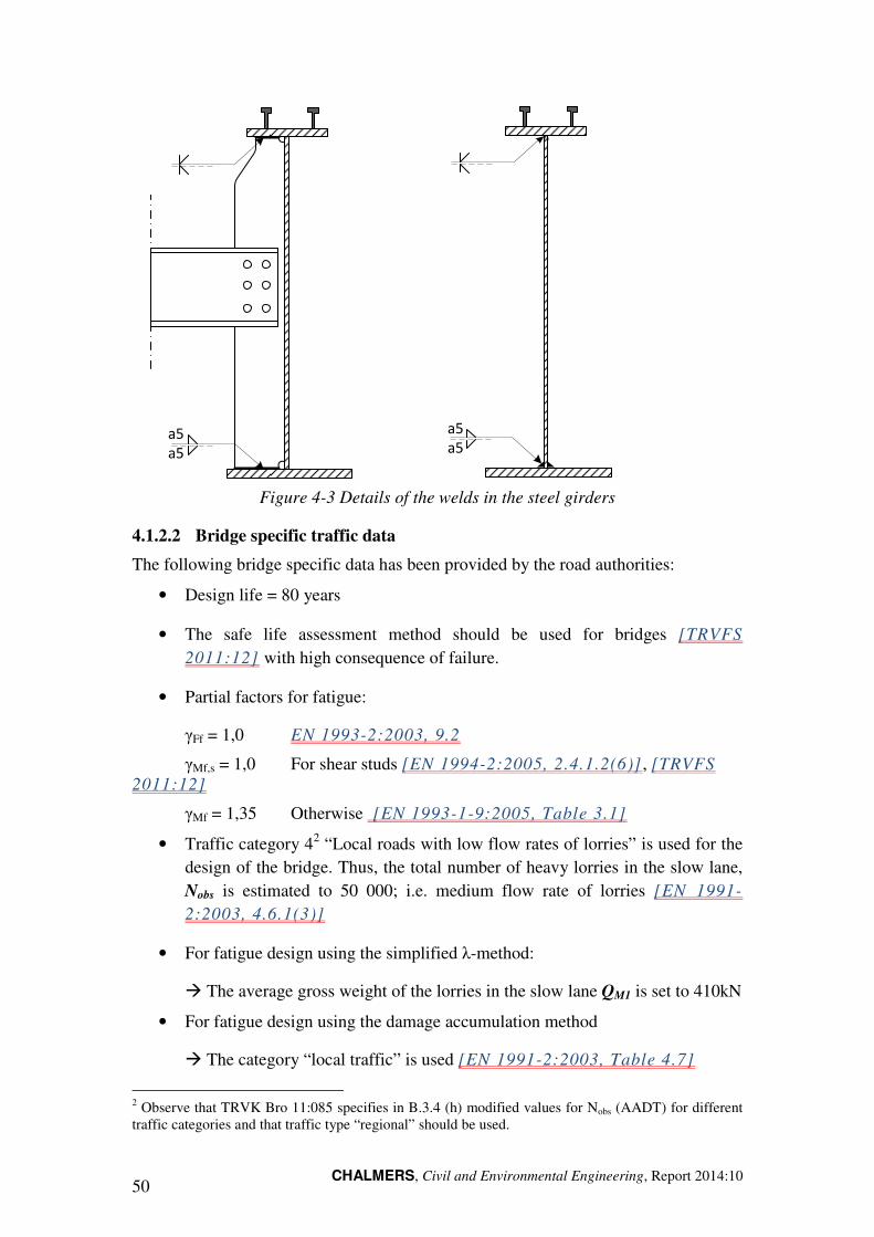
CHALMERS, Civil and Environmental Engineering, Report 2014:10 50
a5
a5
a5
a5
Figure 4-3 Details of the welds in the steel girders
4.1.2.2 Bridge specific traffic data
The following bridge specific data has been provided by the road authorities:
• Design life = 80 years
• The safe life assessment method should be used for bridges [TRVFS 2011:12] with high consequence of failure.
• Partial factors for fatigue:
γFf = 1,0 EN 1993-2:2003, 9.2
γMf,s = 1,0 For shear studs [EN 1994-2:2005, 2.4.1.2(6)] , [TRVFS 2011:12]
γMf = 1,35 Otherwise [EN 1993-1-9:2005, Table 3.1]
• Traffic category 42 “Local roads with low flow rates of lorries” is used for the design of the bridge. Thus, the total number of heavy lorries in the slow lane, Nobs is estimated to 50 000; i.e. medium flow rate of lorries [EN 1991-2:2003, 4.6.1(3)]
• For fatigue design using the simplified λ-method:
� The average gross weight of the lorries in the slow lane QM1 is set to 410kN
• For fatigue design using the damage accumulation method
� The category “local traffic” is used [EN 1991-2:2003, Table 4.7]
2 Observe that TRVK Bro 11:085 specifies in B.3.4 (h) modified values for Nobs (AADT) for different traffic categories and that traffic type “regional” should be used.
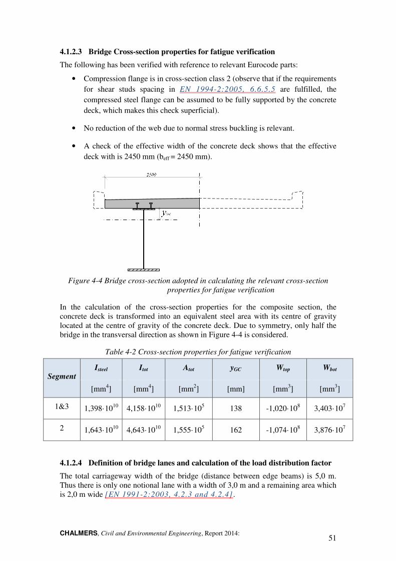
CHALMERS, Civil and Environmental Engineering, Report 2014: 51
4.1.2.3 Bridge Cross-section properties for fatigue verification
The following has been verified with reference to relevant Eurocode parts:
• Compression flange is in cross-section class 2 (observe that if the requirements for shear studs spacing in EN 1994-2:2005, 6.6.5.5 are fulfilled, the compressed steel flange can be assumed to be fully supported by the concrete deck, which makes this check superficial).
• No reduction of the web due to normal stress buckling is relevant.
• A check of the effective width of the concrete deck shows that the effective deck with is 2450 mm (beff = 2450 mm).
Figure 4-4 Bridge cross-section adopted in calculating the relevant cross-section properties for fatigue verification
In the calculation of the cross-section properties for the composite section, the concrete deck is transformed into an equivalent steel area with its centre of gravity located at the centre of gravity of the concrete deck. Due to symmetry, only half the bridge in the transversal direction as shown in Figure 4-4 is considered.
Table 4-2 Cross-section properties for fatigue verification
Segment Isteel Itot Atot yGC Wtop Wbot
[mm4] [mm4] [mm2] [mm] [mm3] [mm3]
1&3 1,398·1010 4,158·1010 1,513·105 138 -1,020·108 3,403·107
2 1,643·1010 4,643·1010 1,555·105 162 -1,074·108 3,876·107
4.1.2.4 Definition of bridge lanes and calculation of the load distribution factor
The total carriageway width of the bridge (distance between edge beams) is 5,0 m. Thus there is only one notional lane with a width of 3,0 m and a remaining area which is 2,0 m wide [EN 1991-2:2003, 4.2.3 and 4.2.4] .
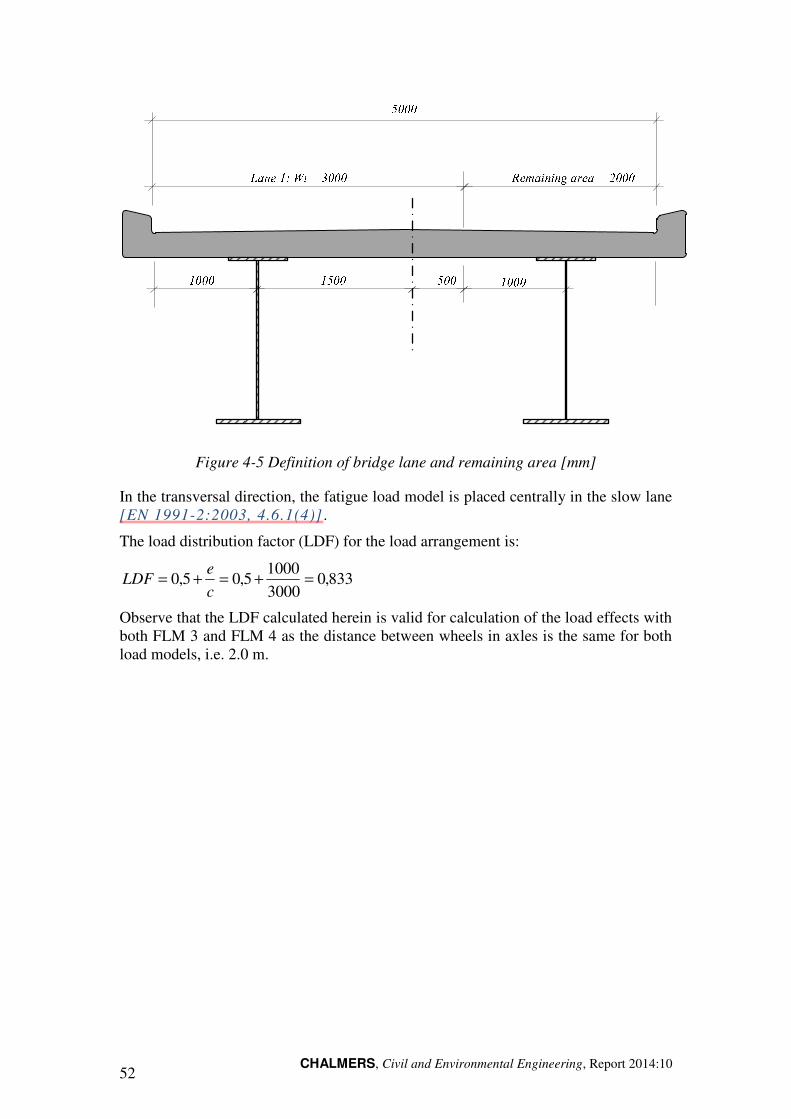
CHALMERS, Civil and Environmental Engineering, Report 2014:10 52
Figure 4-5 Definition of bridge lane and remaining area [mm]
In the transversal direction, the fatigue load model is placed centrally in the slow lane [EN 1991-2:2003, 4.6.1(4)] .
The load distribution factor (LDF) for the load arrangement is:
833,03000
10005,05,0 =+=+=
c
eLDF
Observe that the LDF calculated herein is valid for calculation of the load effects with both FLM 3 and FLM 4 as the distance between wheels in axles is the same for both load models, i.e. 2.0 m.
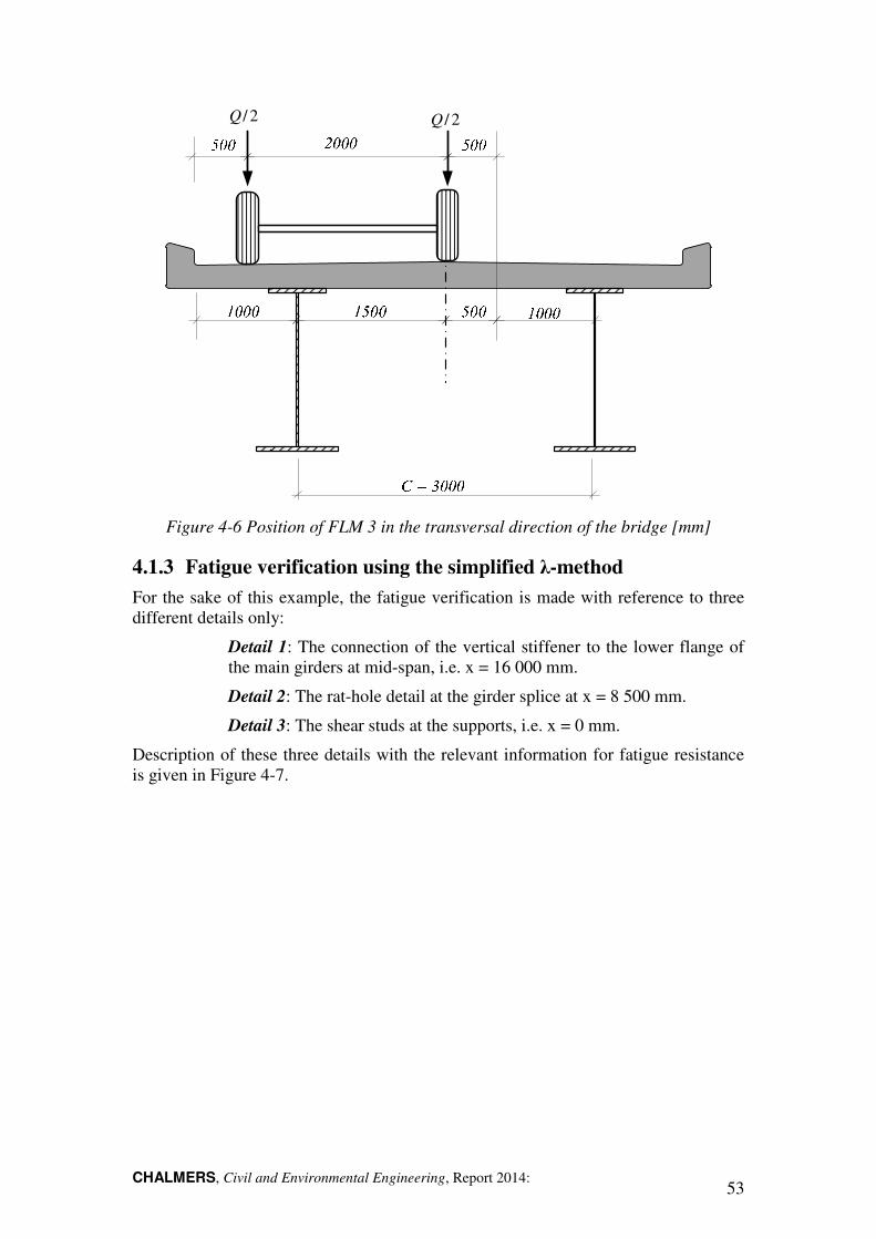
CHALMERS, Civil and Environmental Engineering, Report 2014: 53
2/Q 2/Q
Figure 4-6 Position of FLM 3 in the transversal direction of the bridge [mm]
4.1.3 Fatigue verification using the simplified λ-method
For the sake of this example, the fatigue verification is made with reference to three different details only:
Detail 1: The connection of the vertical stiffener to the lower flange of the main girders at mid-span, i.e. x = 16 000 mm.
Detail 2: The rat-hole detail at the girder splice at x = 8 500 mm.
Detail 3: The shear studs at the supports, i.e. x = 0 mm.
Description of these three details with the relevant information for fatigue resistance is given in Figure 4-7.
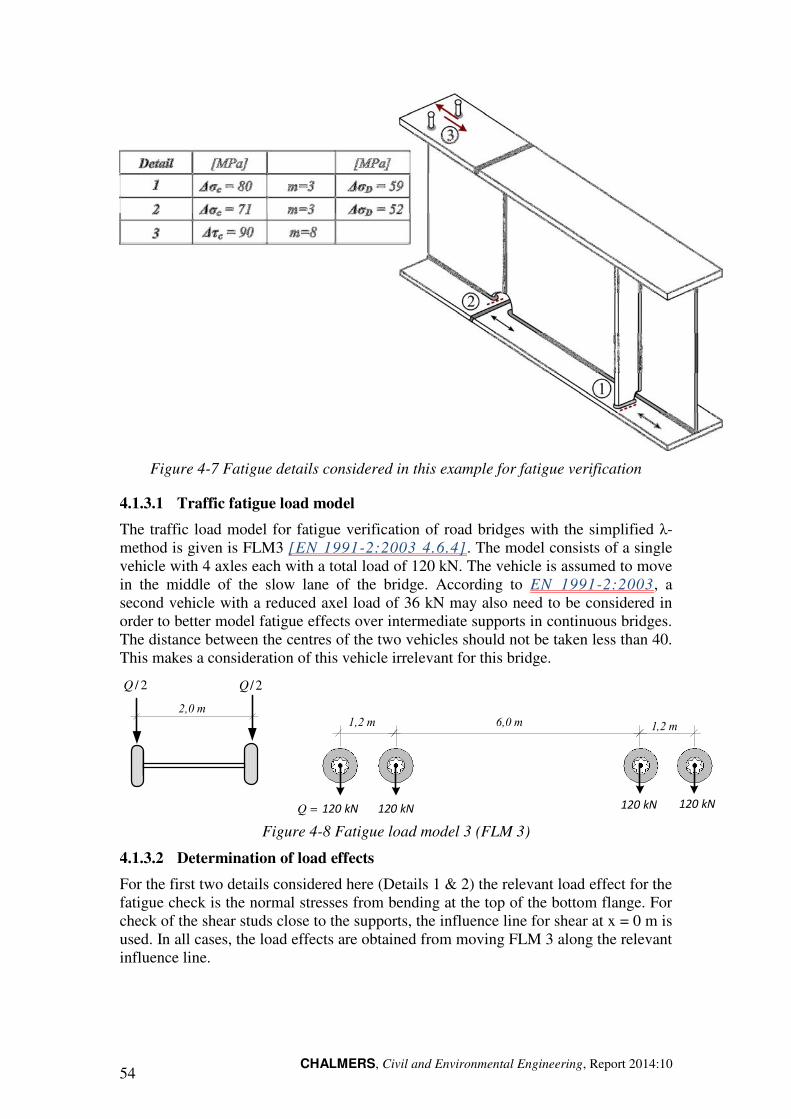
CHALMERS, Civil and Environmental Engineering, Report 2014:10 54
Figure 4-7 Fatigue details considered in this example for fatigue verification
4.1.3.1 Traffic fatigue load model
The traffic load model for fatigue verification of road bridges with the simplified λ-method is given is FLM3 [EN 1991-2:2003 4.6.4] . The model consists of a single vehicle with 4 axles each with a total load of 120 kN. The vehicle is assumed to move in the middle of the slow lane of the bridge. According to EN 1991-2:2003, a second vehicle with a reduced axel load of 36 kN may also need to be considered in order to better model fatigue effects over intermediate supports in continuous bridges. The distance between the centres of the two vehicles should not be taken less than 40. This makes a consideration of this vehicle irrelevant for this bridge.
120 kN120 kN120 kN
2,0 m
2/Q 2/Q
=Q
1,2 m 6,0 m 1,2 m
120 kN
Figure 4-8 Fatigue load model 3 (FLM 3)
4.1.3.2 Determination of load effects
For the first two details considered here (Details 1 & 2) the relevant load effect for the fatigue check is the normal stresses from bending at the top of the bottom flange. For check of the shear studs close to the supports, the influence line for shear at x = 0 m is used. In all cases, the load effects are obtained from moving FLM 3 along the relevant influence line.
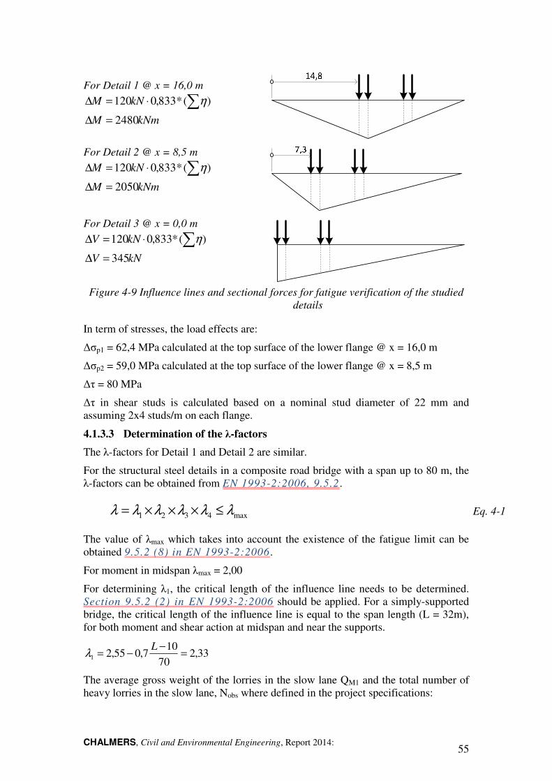
CHALMERS, Civil and Environmental Engineering, Report 2014: 55
For Detail 1 @ x = 16,0 m
kNmM
kNM
2480
)(*833,0120
=∆
⋅=∆ ∑η
For Detail 2 @ x = 8,5 m
kNmM
kNM
2050
)(*833,0120
=∆
⋅=∆ ∑η
For Detail 3 @ x = 0,0 m
kNV
kNV
345
)(*833,0120
=∆
⋅=∆ ∑η
Figure 4-9 Influence lines and sectional forces for fatigue verification of the studied
details
In term of stresses, the load effects are:
∆σp1 = 62,4 MPa calculated at the top surface of the lower flange @ x = 16,0 m
∆σp2 = 59,0 MPa calculated at the top surface of the lower flange @ x = 8,5 m
∆τ = 80 MPa
∆τ in shear studs is calculated based on a nominal stud diameter of 22 mm and assuming 2x4 studs/m on each flange.
4.1.3.3 Determination of the λ-factors
The λ-factors for Detail 1 and Detail 2 are similar.
For the structural steel details in a composite road bridge with a span up to 80 m, the λ-factors can be obtained from EN 1993-2:2006, 9.5.2.
max4321 λλλλλλ ≤×××= Eq. 4-1
The value of λmax which takes into account the existence of the fatigue limit can be obtained 9.5.2 (8) in EN 1993-2:2006.
For moment in midspan λmax = 2,00
For determining λ1, the critical length of the influence line needs to be determined. Section 9.5.2 (2) in EN 1993-2:2006 should be applied. For a simply-supported bridge, the critical length of the influence line is equal to the span length (L = 32m), for both moment and shear action at midspan and near the supports.
33,270
107,055,21 =
−−=
Lλ
The average gross weight of the lorries in the slow lane QM1 and the total number of heavy lorries in the slow lane, Nobs where defined in the project specifications:
CHALMERS, Civil and Environmental Engineering, Report 2014:10 56
kNQM 4101 =
31050 ⋅=obsN
With the reference values as given in [EN 1993-2:2006, 9.5.2 (3)] :
kNQ 4800 =
30 10500 ⋅=N
Thus the factor for traffic volume is:
539,051
00
12 =
=
N
N
Q
Q obsMλ
The design life of the bridge is 80 years which gives a correction factor:
956,0100
80 51
3 =
=λ , which is according to [EN 1993-2:2006, 9.5.2 (5)] .
The bridge has only one traffic lane, thus:
0,14 =λ
The total λ-factors with reference to Detail 1 and Detail 2 becomes
201,10,1956,0539,033,24 =⋅⋅⋅=λ
Which is less than λmax = 2,0
Fatigue verification of shear studs (Detail 3) is treated in EN 1994-2:2005. The verification condition reads:
sMf
cEFf
,2,
γ
ττγ
∆≤∆⋅ Eq. 4-2
where,
τλτ ∆⋅=∆ vE 2, , MPac 90=∆τ
and
4,3,2,1, vvvvv λλλλλ ×××= Eq. 4-3
For road bridges with spans up to 100 m, λv,1 should be taken as 1.55 [EN 1994-2:2005, 6.8.6.1(4)] .
The other factors, λv,2 to λv,4 are obtained from EN 1993-2:2006. However, the fatigue strength curve (S-N curve) for shear studs loaded in shear has a slope of 1:8 (i.e. m = 8) and thus the λ-factors for shear studs need to be corrected with reference to that. That is made by replacing the exponent 1/5 with 1/8 in the expressions for λv2 to λv4.
CHALMERS, Civil and Environmental Engineering, Report 2014: 57
Therefore:
81
00
12,
=
NN
QQ obsM
vλ � 641,05,005,0
480410 8
1
2, =
=vλ
973,010080 8
1
3, =
=vλ
0,13, =vλ
967,00,1973,0641,0550,1 =⋅⋅⋅=vλ
The dynamic amplification factor is included in the fatigue load model FLM 3, therefore ϕ2 = 1,0.
4.1.3.4 Fatigue verification
For each detail, the fatigue verification can now be performed by comparing the equivalent stress range at 2 million cycles (∆σE,2 or ∆τE,2) with the fatigue strength of each detail accounting for relevant partial factor for fatigue resistance (γMf).
In addition to the fatigue check in this format, a damage accumulation factor can also be derived for example from A.6 in EN 1993-1-9:2005. The damage factor can be expressed as:
3
2,
∆
∆⋅=
MfD
EFfDγσ
σγ Eq. 4-4
For Detail 1:
MPapE 9,7422, =∆⋅⋅=∆ σφλσ
The corresponding fatigue resistance at 2 million cycles (i.e. the fatigue strength):
MPaC 80=∆σ
And the verification reads:
0,1264,12,>=
∆
∆⋅⋅
C
EMfFf
σ
σγγ
and the corresponding damage factor is:
0,102,23
2,>=
∆
∆⋅⋅=
C
EMfFfDσ
σγγ
For Detail 2:
MPapE 5,7122, =∆⋅⋅=∆ σφλσ
and
CHALMERS, Civil and Environmental Engineering, Report 2014:10 58
MPaC 71=∆σ
And the verification reads:
0,1359,12,>=
∆
∆⋅⋅
C
EMfFf
σ
σγγ
With a corresponding damage factor:
512,23
2,=
∆
∆⋅⋅=
C
EMfFfDσ
σγγ
Detail 3:
The shear stress range in each stud is ∆τ = 80 MPa (see 4.2 above), thus:
τλτ ∆⋅=∆ vE 2,
MPaE 4,7780967,02, =×=∆τ
With γMf,s = 1,0 as recommended in TRVFS 2011:12, the verification reads:
0,190
4,770,1 ≤⋅
which is satisfied. The required number of shear studs with reference to fatigue may
be calculated as:
1084,77
90=⋅=studsn
Observe that the number of shear studs close to the supports of simply-supported
bridge is usually determined by the requirements in the ULS, while the fatigue
verification governs by the number of shear studs in mid-span region.
4.1.4 Fatigue verification using the Damage Accumulation method
Eurocode allows for fatigue verification of road and railway bridges to be performed using the cumulative damage method. For this purpose, EN 1991-2 provides load models for both road bridges (EN 1991-2:2003, 4.6.5) and railway bridges (EN 1991-2:2003, D.3). For the purpose of illustration, the method is applied here to verify the fatigue strength of Detail 1.
For road bridges, fatigue load model 4 (FLM 4) should be used for calculating the total fatigue damage accumulated through the design service life of the bridge. This fatigue load model is composed of 5 different vehicles (lorries) which are meant to represent the real traffic composition on road bridges in a more accurate way. Detailed information about the composition of FLM4 can be found in Table 4.7 in EN 1991-2:2003.
Verification of the fatigue strength of Detail 1 in this example is performed according to the following steps:
1. Relevant data for the fatigue strength of the detail is established
CHALMERS, Civil and Environmental Engineering, Report 2014: 59
2. The stress history is determined by moving each vehicle in FLM 4 individually along the bridge, in the centre of the traffic lane (thus, the load effects need to be modified with relevant LDF, see Section 4.1.2.4 in this example).
3. The stress histogram is constructed using appropriate method (for example the reservoir method).
4. The damage caused by individual blocks in the stress histogram is calculated (accounting for the slope of the S-N curve) and all damage components are summed to obtain a total damage.
5. Verification is made by checking the condition Dtot ≤ 1,0.
In this simple example (a simply supported bridge) the stress history from each lorry passage and the resultant stress histogram are obtained by hand calculations.
4.1.4.1 Fatigue strength curve
The fatigue strength curve for Detail 1 is shown in Figure 4-10. Detail Category 80 applies as given for Detail 7 in EN 1993-1-9:2005, Table 8.4 assuming that the thickness of the vertical stiffener with the fillet welds on each side is less than 50 mm. Thus:
∆σc=80,0 MPa
∆σD=59,0 MPa
∆σL=32,0 MPa
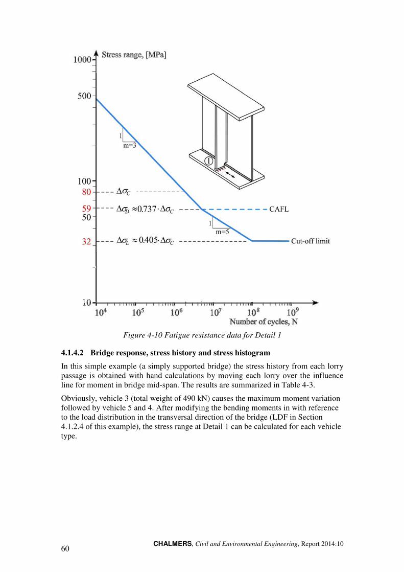
CHALMERS, Civil and Environmental Engineering, Report 2014:10 60
Figure 4-10 Fatigue resistance data for Detail 1
4.1.4.2 Bridge response, stress history and stress histogram
In this simple example (a simply supported bridge) the stress history from each lorry passage is obtained with hand calculations by moving each lorry over the influence line for moment in bridge mid-span. The results are summarized in Table 4-3.
Obviously, vehicle 3 (total weight of 490 kN) causes the maximum moment variation followed by vehicle 5 and 4. After modifying the bending moments in with reference to the load distribution in the transversal direction of the bridge (LDF in Section 4.1.2.4 of this example), the stress range at Detail 1 can be calculated for each vehicle type.
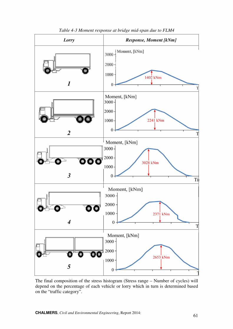
CHALMERS, Civil and Environmental Engineering, Report 2014: 61
Table 4-3 Moment response at bridge mid-span due to FLM4
Lorry Response, Moment [kNm]
1
2
3
4
5
The final composition of the stress histogram (Stress range – Number of cycles) will depend on the percentage of each vehicle or lorry which in turn is determined based on the “traffic category”.
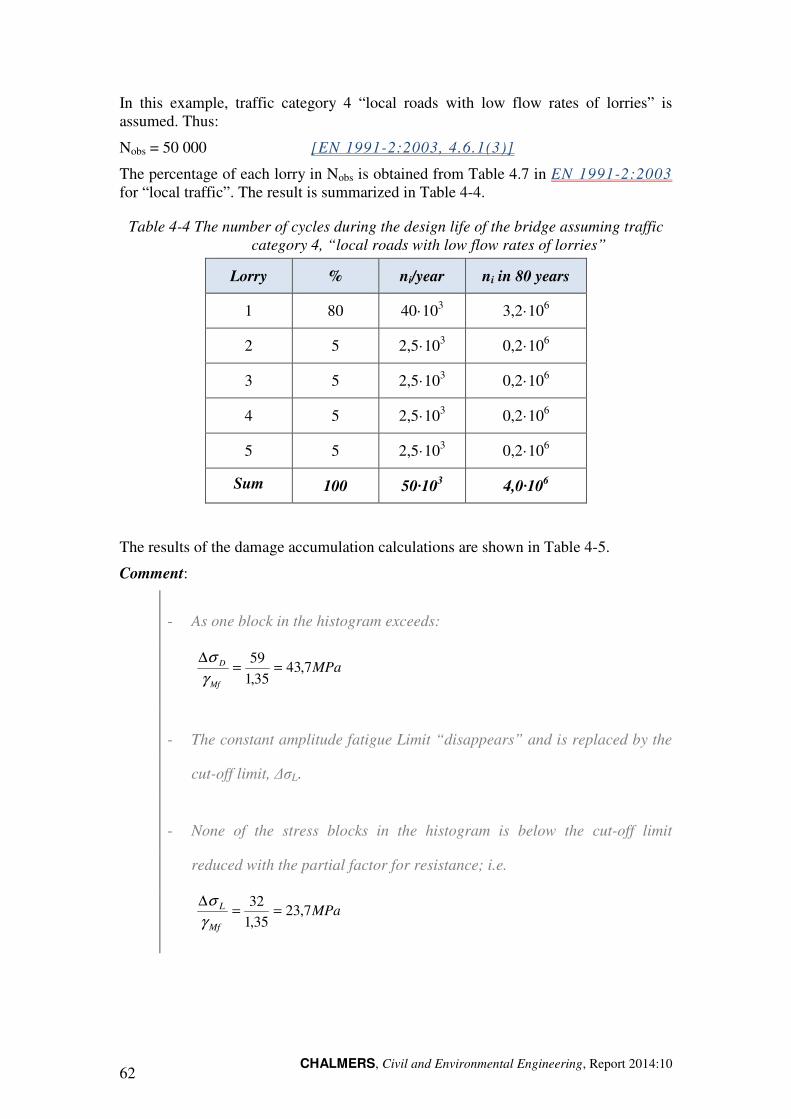
CHALMERS, Civil and Environmental Engineering, Report 2014:10 62
In this example, traffic category 4 “local roads with low flow rates of lorries” is assumed. Thus:
Nobs = 50 000 [EN 1991-2:2003, 4.6.1(3)]
The percentage of each lorry in Nobs is obtained from Table 4.7 in EN 1991-2:2003 for “local traffic”. The result is summarized in Table 4-4.
Table 4-4 The number of cycles during the design life of the bridge assuming traffic category 4, “local roads with low flow rates of lorries”
Lorry % ni/year ni in 80 years
1 80 40·103 3,2·106
2 5 2,5·103 0,2·106
3 5 2,5·103 0,2·106
4 5 2,5·103 0,2·106
5 5 2,5·103 0,2·106
Sum 100 50·103 4,0·106
The results of the damage accumulation calculations are shown in Table 4-5.
Comment:
- As one block in the histogram exceeds:
MPaMf
D 7,4335,1
59==
∆
γ
σ
- The constant amplitude fatigue Limit “disappears” and is replaced by the
cut-off limit, ∆σL.
- None of the stress blocks in the histogram is below the cut-off limit
reduced with the partial factor for resistance; i.e.
MPaMf
L 7,2335,1
32==
∆
γ
σ
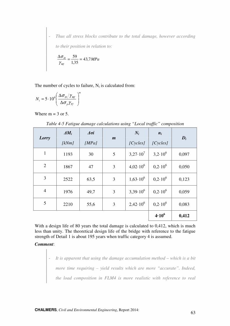
CHALMERS, Civil and Environmental Engineering, Report 2014: 63
- Thus all stress blocks contribute to the total damage, however according
to their position in relation to:
MPaMf
D 7,4335,1
59==
∆
γ
σ
The number of cycles to failure, Ni is calculated from: m
Ffp
MfDiN
∆
∆⋅=
γσ
γσ6105
Where m = 3 or 5.
Table 4-5 Fatigue damage calculations using “Local traffic” composition
Lorry ∆Mi ∆σi
m Ni ni
Di [kNm] [MPa] [Cycles] [Cycles]
1 1193 30 5 3,27·107 3,2·106 0,097
2 1867 47 3 4,02·106 0,2·106 0,050
3 2522 63,5 3 1,63·106 0,2·106 0,123
4 1976 49,7 3 3,39·106 0,2·106 0,059
5 2210 55,6 3 2,42·106 0,2·106 0,083
4·106 0,412
With a design life of 80 years the total damage is calculated to 0,412, which is much less than unity. The theoretical design life of the bridge with reference to the fatigue strength of Detail 1 is about 195 years when traffic category 4 is assumed.
Comment:
- It is apparent that using the damage accumulation method – which is a bit
more time requiring – yield results which are more “accurate”. Indeed,
the load composition in FLM4 is more realistic with reference to real
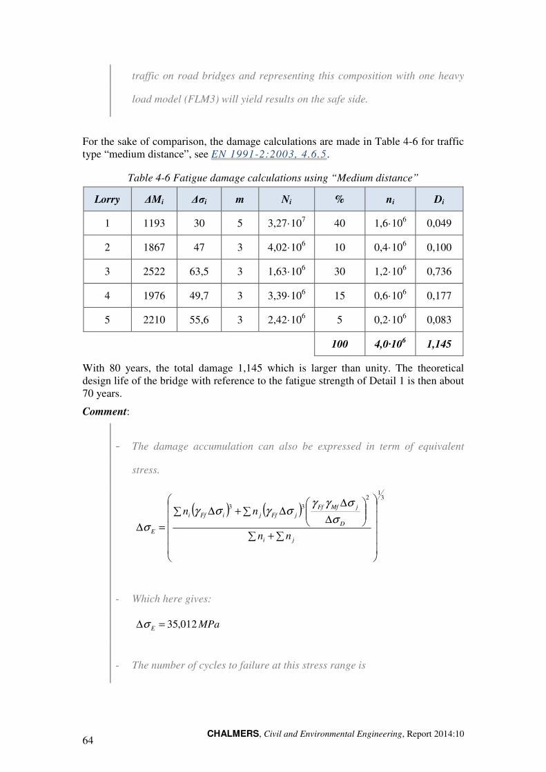
CHALMERS, Civil and Environmental Engineering, Report 2014:10 64
traffic on road bridges and representing this composition with one heavy
load model (FLM3) will yield results on the safe side.
For the sake of comparison, the damage calculations are made in Table 4-6 for traffic type “medium distance”, see EN 1991-2:2003, 4.6.5.
Table 4-6 Fatigue damage calculations using “Medium distance”
Lorry ∆Mi ∆σi m Ni % ni Di
1 1193 30 5 3,27·107 40 1,6·106 0,049
2 1867 47 3 4,02·106 10 0,4·106 0,100
3 2522 63,5 3 1,63·106 30 1,2·106 0,736
4 1976 49,7 3 3,39·106 15 0,6·106 0,177
5 2210 55,6 3 2,42·106 5 0,2·106 0,083
100 4,0·106 1,145
With 80 years, the total damage 1,145 which is larger than unity. The theoretical design life of the bridge with reference to the fatigue strength of Detail 1 is then about 70 years.
Comment:
- The damage accumulation can also be expressed in term of equivalent
stress.
( ) ( )3
12
33
∑+∑
∆
∆∆∑+∆∑
=∆ji
D
jMfFfjFfjiFfi
E nn
nnσ
σγγσγσγ
σ
- Which here gives:
MPaE 012,35=∆σ
- The number of cycles to failure at this stress range is
CHALMERS, Civil and Environmental Engineering, Report 2014: 65
CyclesNEFf
Mf
D
E6
3
6 107059105 ⋅=
∆⋅
∆
⋅⋅=σγ
γ
σ
- And the total damage becomes:
412,0=∑
=E
ii
N
nD
- Which is the same damage sum obtained in Table 4-5 above.
Comment:
- A fatigue verification following the same format used in the simplified λ-
method can be derived from the damage accumulation calculations:
- With: ∆σE=35,012MPa
MPan
ii
EE 112,44102
3
62, =
⋅
∑⋅∆=∆ σσ
- And the verification reads
Satisfied∆σ
∆σγγ
C
E,FfMf 0,1744,02<=
⋅⋅
- Again this yields the same damage factor, D:
412,03
2=
⋅⋅=
C
E,FfMf
∆σ
∆σγγD
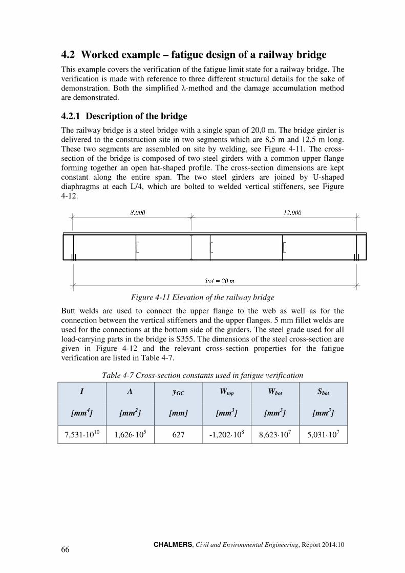
CHALMERS, Civil and Environmental Engineering, Report 2014:10 66
4.2 Worked example – fatigue design of a railway bridge
This example covers the verification of the fatigue limit state for a railway bridge. The verification is made with reference to three different structural details for the sake of demonstration. Both the simplified λ-method and the damage accumulation method are demonstrated.
4.2.1 Description of the bridge
The railway bridge is a steel bridge with a single span of 20,0 m. The bridge girder is delivered to the construction site in two segments which are 8,5 m and 12,5 m long. These two segments are assembled on site by welding, see Figure 4-11. The cross-section of the bridge is composed of two steel girders with a common upper flange forming together an open hat-shaped profile. The cross-section dimensions are kept constant along the entire span. The two steel girders are joined by U-shaped diaphragms at each L/4, which are bolted to welded vertical stiffeners, see Figure 4-12.
Figure 4-11 Elevation of the railway bridge
Butt welds are used to connect the upper flange to the web as well as for the connection between the vertical stiffeners and the upper flanges. 5 mm fillet welds are used for the connections at the bottom side of the girders. The steel grade used for all load-carrying parts in the bridge is S355. The dimensions of the steel cross-section are given in Figure 4-12 and the relevant cross-section properties for the fatigue verification are listed in Table 4-7.
Table 4-7 Cross-section constants used in fatigue verification
I A yGC Wtop Wbot Sbot
[mm4] [mm2] [mm] [mm3] [mm3] [mm3]
7,531·1010 1,626·105 627 -1,202·108 8,623·107 5,031·107

CHALMERS, Civil and Environmental Engineering, Report 2014: 67
Figure 4-12 Cross-section of the bridge
4.2.2 Bridge specific traffic data
The following bridge specific data has been adopted in this example:
• Design life = 120 years
• The safe life assessment method should be used for bridges [BFS 2011:10] with high consequence of failure.
� Partial factors for fatigue
γFf = 1,0 1993-2: 9.2
γMf = 1,35 Otherwise [1993-1-9:2005, Table 3.1]
• Rail traffic with 25 t axels is used for fatigue verification [1993-2:2006, 9.5.3].
• The traffic per year is specified to 25 million tonnes per track
• Carefully maintained track is assumed
4.2.3 Fatigue verification using the simplified λ-method
For the sake of this example, the fatigue verification is made with reference to three different details only:
Detail 1: The connection of the vertical stiffener to the lower flange of the main girders at mid-span, i.e. x = 10,0 m.
Detail 2: The rat-hole detail at the girder splice @ x = 8,0 m.
Detail 3: Connection of welded stiffener to girder web @ x = 5,0 m.
Description of these three details with the relevant information for fatigue resistance is given in Figure 4-13 and Table 4-8.
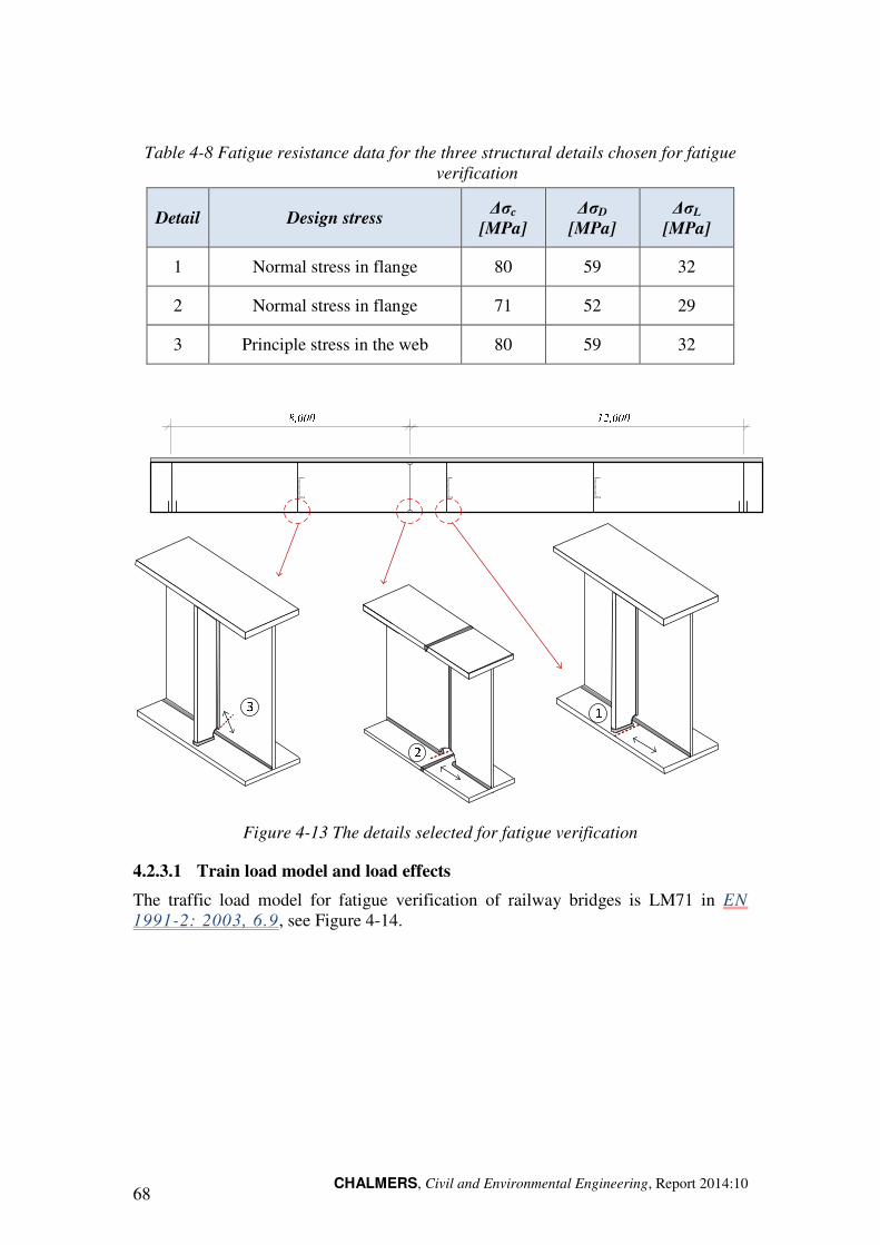
CHALMERS, Civil and Environmental Engineering, Report 2014:10 68
Table 4-8 Fatigue resistance data for the three structural details chosen for fatigue verification
Detail Design stress ∆σc
[MPa] ∆σD
[MPa] ∆σL
[MPa]
1 Normal stress in flange 80 59 32
2 Normal stress in flange 71 52 29
3 Principle stress in the web 80 59 32
Figure 4-13 The details selected for fatigue verification
4.2.3.1 Train load model and load effects
The traffic load model for fatigue verification of railway bridges is LM71 in EN 1991-2: 2003, 6.9, see Figure 4-14.
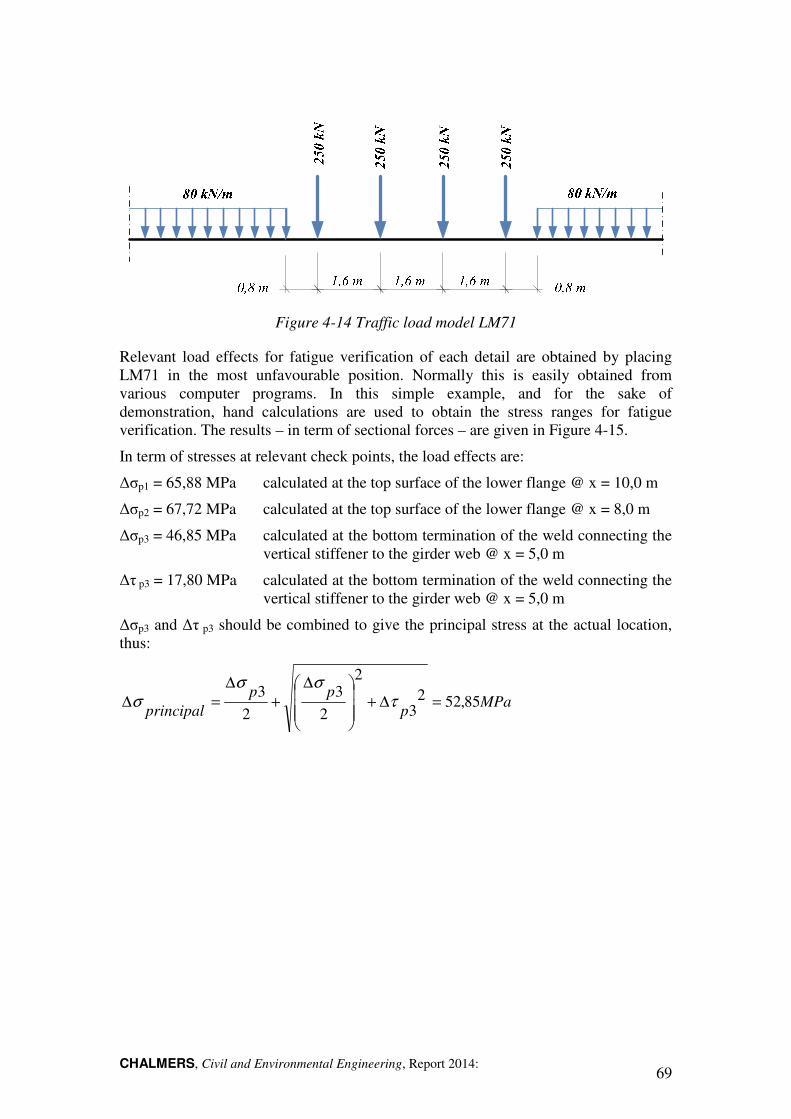
CHALMERS, Civil and Environmental Engineering, Report 2014: 69
Figure 4-14 Traffic load model LM71
Relevant load effects for fatigue verification of each detail are obtained by placing LM71 in the most unfavourable position. Normally this is easily obtained from various computer programs. In this simple example, and for the sake of demonstration, hand calculations are used to obtain the stress ranges for fatigue verification. The results – in term of sectional forces – are given in Figure 4-15.
In term of stresses at relevant check points, the load effects are:
∆σp1 = 65,88 MPa calculated at the top surface of the lower flange @ x = 10,0 m
∆σp2 = 67,72 MPa calculated at the top surface of the lower flange @ x = 8,0 m
∆σp3 = 46,85 MPa calculated at the bottom termination of the weld connecting the vertical stiffener to the girder web @ x = 5,0 m
∆τ p3 = 17,80 MPa calculated at the bottom termination of the weld connecting the vertical stiffener to the girder web @ x = 5,0 m
∆σp3 and ∆τ p3 should be combined to give the principal stress at the actual location, thus:
MPap
ppprincipal
85,5223
2
23
23
=∆+
∆+
∆=∆ τ
σσσ
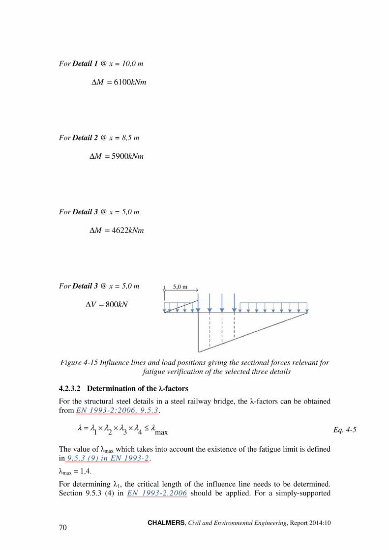
CHALMERS, Civil and Environmental Engineering, Report 2014:10 70
For Detail 1 @ x = 10,0 m
kNmM 6100=∆
For Detail 2 @ x = 8,5 m
kNmM 5900=∆
For Detail 3 @ x = 5,0 m
kNmM 4622=∆
For Detail 3 @ x = 5,0 m
kNV 800=∆
Figure 4-15 Influence lines and load positions giving the sectional forces relevant for fatigue verification of the selected three details
4.2.3.2 Determination of the λ-factors
For the structural steel details in a steel railway bridge, the λ-factors can be obtained from EN 1993-2:2006, 9.5.3.
max4321λλλλλλ ≤×××= Eq. 4-5
The value of λmax which takes into account the existence of the fatigue limit is defined in 9.5.3 (9) in EN 1993-2.
λmax = 1,4.
For determining λ1, the critical length of the influence line needs to be determined. Section 9.5.3 (4) in EN 1993-2.2006 should be applied. For a simply-supported
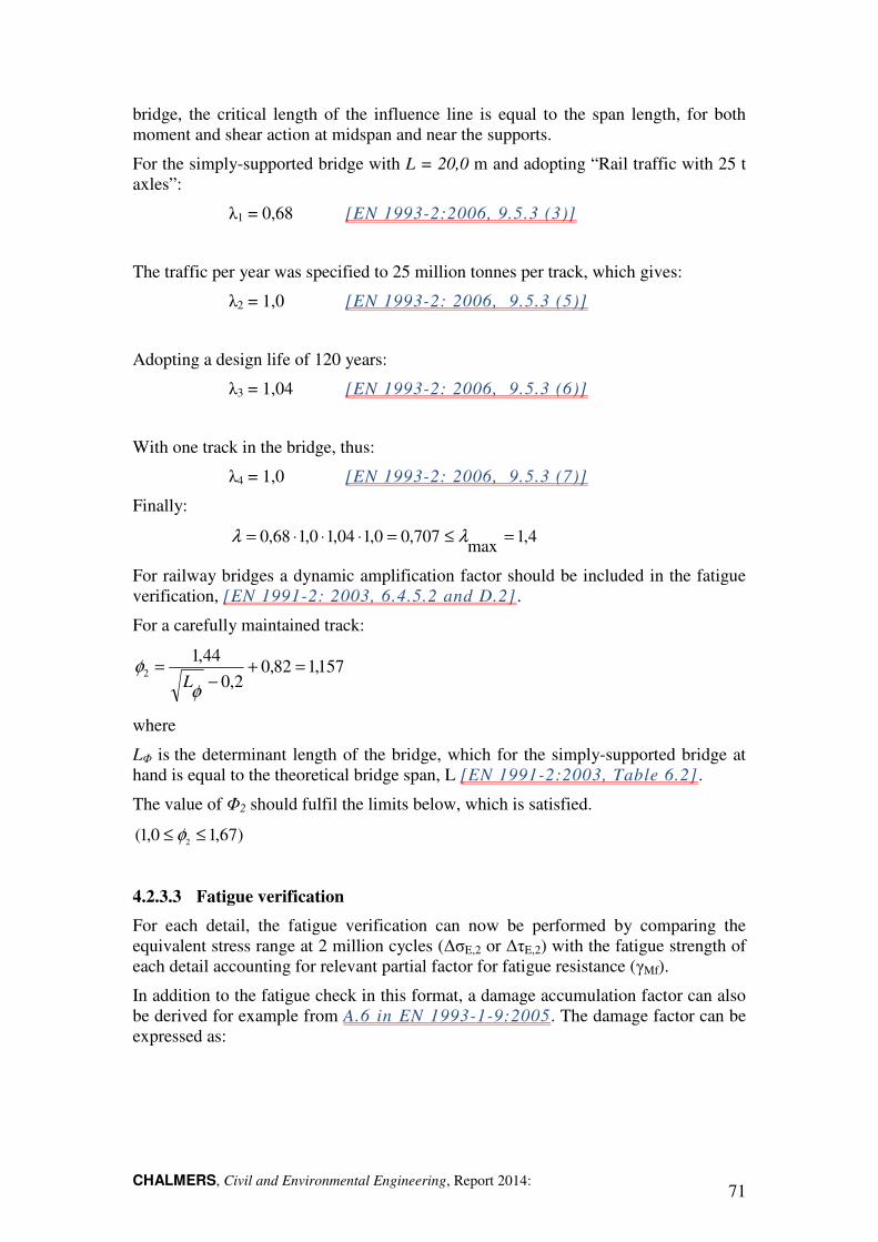
CHALMERS, Civil and Environmental Engineering, Report 2014: 71
bridge, the critical length of the influence line is equal to the span length, for both moment and shear action at midspan and near the supports.
For the simply-supported bridge with L = 20,0 m and adopting “Rail traffic with 25 t axles”:
λ1 = 0,68 [EN 1993-2:2006, 9.5.3 (3)]
The traffic per year was specified to 25 million tonnes per track, which gives:
λ2 = 1,0 [EN 1993-2: 2006, 9.5.3 (5)]
Adopting a design life of 120 years:
λ3 = 1,04 [EN 1993-2: 2006, 9.5.3 (6)]
With one track in the bridge, thus:
λ4 = 1,0 [EN 1993-2: 2006, 9.5.3 (7)]
Finally:
4,1max
707,00,104,10,168,0 =≤=⋅⋅⋅= λλ
For railway bridges a dynamic amplification factor should be included in the fatigue verification, [EN 1991-2: 2003, 6.4.5.2 and D.2] .
For a carefully maintained track:
157,182,02,0
44,12 =+
−=
φ
φL
where
LΦ is the determinant length of the bridge, which for the simply-supported bridge at hand is equal to the theoretical bridge span, L [EN 1991-2:2003, Table 6.2] .
The value of Φ2 should fulfil the limits below, which is satisfied.
)67,10,1( 2 ≤≤ φ
4.2.3.3 Fatigue verification
For each detail, the fatigue verification can now be performed by comparing the equivalent stress range at 2 million cycles (∆σE,2 or ∆τE,2) with the fatigue strength of each detail accounting for relevant partial factor for fatigue resistance (γMf).
In addition to the fatigue check in this format, a damage accumulation factor can also be derived for example from A.6 in EN 1993-1-9:2005. The damage factor can be expressed as:

CHALMERS, Civil and Environmental Engineering, Report 2014:10 72
3
2
⋅⋅=
C
E,FfMfeq
∆σ
∆σγγD Eq. 4-6
For Detail 1
MPap 88,651 =∆σ MPaE 9,5388,65157,1707,02, =⋅⋅=∆σ
The fatigue verification reads:
0,191,00,180
9,5335,12,≤=
⋅=
∆
∆⋅
MfC
EFf
γσ
σγ
In term of equivalent damage, the result is:
753,080
9,5335,10,13
=
⋅⋅=eqD
Following the same principles, the other two details are treated. The results are summarized in Table 4-9.
Table 4-9 Results from fatigue verification of the selected details according to the λ-method
Detail 1
∆σE,2 53,9 52,1 43,25
∆σc 80 71 80
λ-verification 0,91 0,99 0,73
Deq 0,753 0,974 0,389
4.3 Fatigue verification using the Damage Accumulation
method
Eurocode allows for fatigue verification of road and railway bridges to be performed using the cumulative damage method. For this purpose, EN 1991-2:2003 provides the relevant load models for railway bridges in Annex D.3. For the purpose of illustration, the method is applied here to verify the fatigue strength of the selected
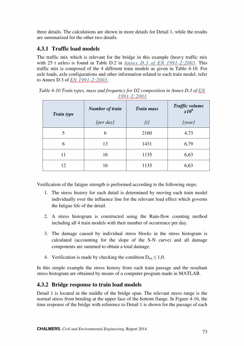
CHALMERS, Civil and Environmental Engineering, Report 2014: 73
three details. The calculations are shown in more details for Detail 1, while the results are summarized for the other two details.
4.3.1 Traffic load models
The traffic mix which is relevant for the bridge in this example (heavy traffic mix with 25 t axles) is found in Table D.2 in Annex D.3 of EN 1991-2:2003. This traffic mix is composed of the 4 different train models as given in Table 4-10. For axle loads, axle configurations and other information related to each train model, refer to Annex D.3 of EN 1991-2:2003.
Table 4-10 Train types, mass and frequency for D2 composition in Annex D.3 of EN 1991-2:2003
Train type Number of train Train mass
Traffic volume x106
[per day] [t] [year]
5 6 2160 4,73
6 13 1431 6,79
11 16 1135 6,63
12 16 1135 6,63
Verification of the fatigue strength is performed according to the following steps:
1. The stress history for each detail is determined by moving each train model individually over the influence line for the relevant load effect which governs the fatigue life of the detail.
2. A stress histogram is constructed using the Rain-flow counting method including all 4 train models with their number of occurrence per day.
3. The damage caused by individual stress blocks in the stress histogram is calculated (accounting for the slope of the S-N curve) and all damage components are summed to obtain a total damage.
4. Verification is made by checking the condition Dtot ≤ 1,0.
In this simple example the stress history from each train passage and the resultant stress histogram are obtained by means of a computer program made in MATLAB.
4.3.2 Bridge response to train load models
Detail 1 is located in the middle of the bridge span. The relevant stress range is the normal stress from bending at the upper face of the bottom flange. In Figure 4-16, the time response of the bridge with reference to Detail 1 is shown for the passage of each

CHALMERS, Civil and Environmental Engineering, Report 2014:10 74
train model in the studied composition. The results from the damage accumulation calculations are listed in Table 4-11.
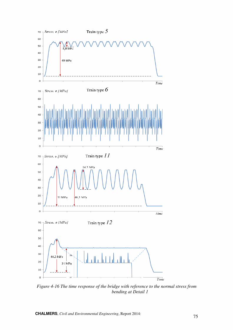
CHALMERS, Civil and Environmental Engineering, Report 2014: 75
Figure 4-16 The time response of the bridge with reference to the normal stress from
bending at Detail 1
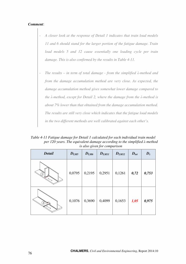
CHALMERS, Civil and Environmental Engineering, Report 2014:10 76
Comment:
- A closer look at the response of Detail 1 indicates that train load models
11 and 6 should stand for the larger portion of the fatigue damage. Train
load models 5 and 12 cause essentially one loading cycle per train
damage. This is also confirmed by the results in Table 4-11.
- The results – in term of total damage - from the simplified λ-method and
from the damage accumulation method are very close. As expected, the
damage accumulation method gives somewhat lower damage compared to
the λ-method, except for Detail 2, where the damage from the λ-method is
about 7% lower than that obtained from the damage accumulation method.
The results are still very close which indicates that the fatigue load models
in the two different methods are well calibrated against each other’s.
Table 4-11 Fatigue damage for Detail 1 calculated for each individual train model per 120 years. The equivalent damage according to the simplified λ-method
is also given for comparison
Detail DLM5 DLM6 DLM11 DLM12 Dtot Dλ
1
0,0795 0,2195 0,2951 0,1261 0,72 0,753
0,1076 0,3690 0,4099 0,1653 1,05 0,975
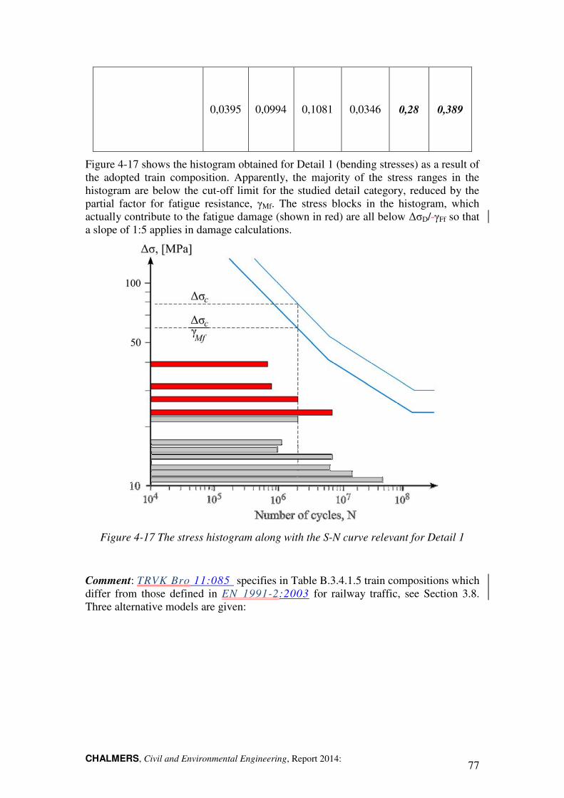
CHALMERS, Civil and Environmental Engineering, Report 2014: 77
0,0395 0,0994 0,1081 0,0346 0,28 0,389
Figure 4-17 shows the histogram obtained for Detail 1 (bending stresses) as a result of the adopted train composition. Apparently, the majority of the stress ranges in the histogram are below the cut-off limit for the studied detail category, reduced by the partial factor for fatigue resistance, γMf. The stress blocks in the histogram, which actually contribute to the fatigue damage (shown in red) are all below ∆σD/ γFf so that a slope of 1:5 applies in damage calculations.
Figure 4-17 The stress histogram along with the S-N curve relevant for Detail 1
Comment: TRVK Bro 11:085 specifies in Table B.3.4.1.5 train compositions which differ from those defined in EN 1991-2:2003 for railway traffic, see Section 3.8. Three alternative models are given:
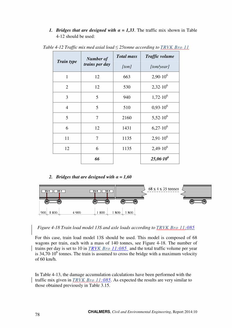
CHALMERS, Civil and Environmental Engineering, Report 2014:10 78
1. Bridges that are designed with α = 1,33. The traffic mix shown in Table 4-12 should be used:
Table 4-12 Traffic mix med axial load ≤ 25tonne according to TRVK Bro 11
Train type Number of trains per day
Total mass Traffic volume
[ton] [ton/year]
1 12 663 2,90·106
2 12 530 2,32·106
3 5 940 1,72·106
4 5 510 0,93·106
5 7 2160 5,52·106
6 12 1431 6,27·106
11 7 1135 2,91·106
12 6 1135 2,49·106
66 25,06·106
2. Bridges that are designed with α = 1,60
Figure 4-18 Train load model 13S and axle loads according to TRVK Bro 11:085
For this case, train load model 13S should be used. This model is composed of 68 wagons per train, each with a mass of 140 tonnes, see Figure 4-18. The number of trains per day is set to 10 in TRVK Bro 11:085 and the total traffic volume per year is 34,70·106 tonnes. The train is assumed to cross the bridge with a maximum velocity of 60 km/h.
In Table 4-13, the damage accumulation calculations have been performed with the traffic mix given in TRVK Bro 11:085. As expected the results are very similar to those obtained previously in Table 3.15.
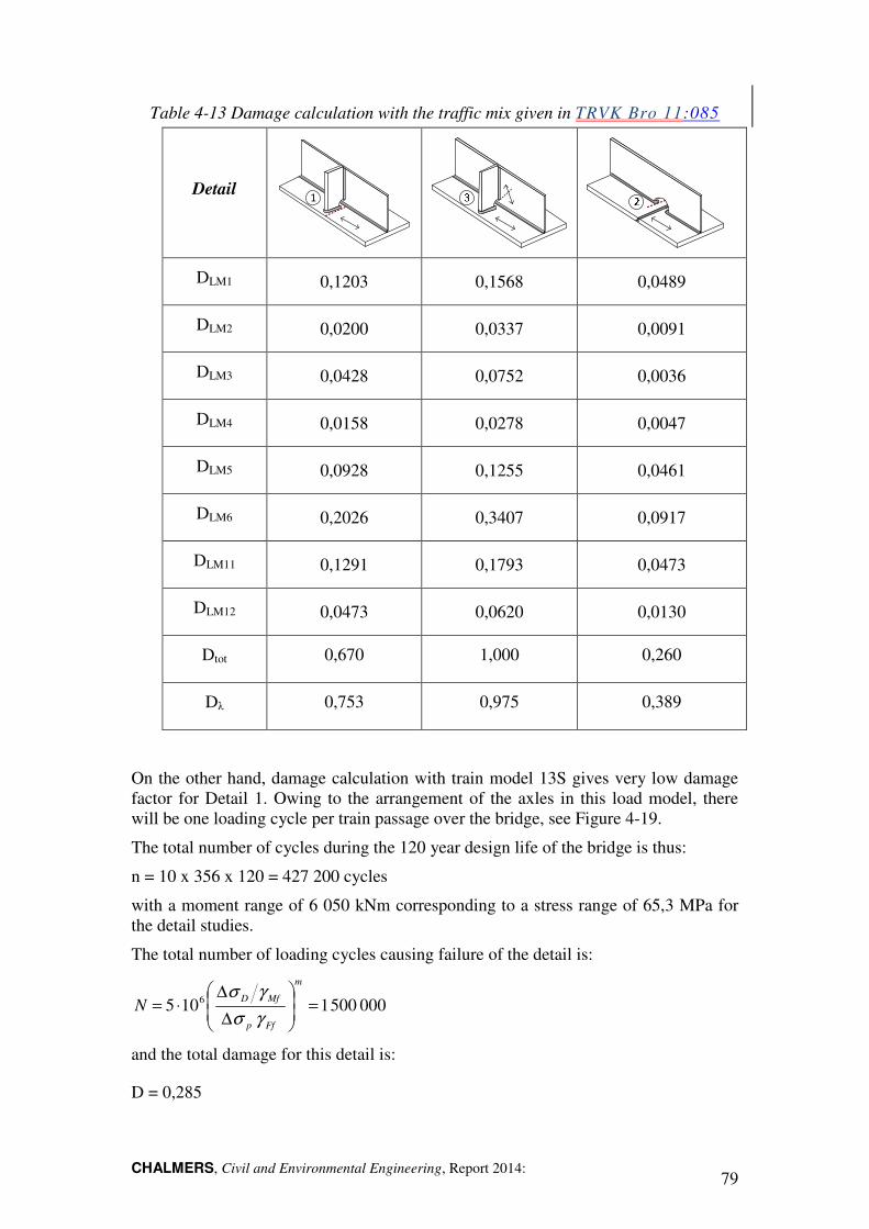
CHALMERS, Civil and Environmental Engineering, Report 2014: 79
Table 4-13 Damage calculation with the traffic mix given in TRVK Bro 11:085
Detail 1
DLM1 0,1203 0,1568 0,0489
DLM2 0,0200 0,0337 0,0091
DLM3 0,0428 0,0752 0,0036
DLM4 0,0158 0,0278 0,0047
DLM5 0,0928 0,1255 0,0461
DLM6 0,2026 0,3407 0,0917
DLM11 0,1291 0,1793 0,0473
DLM12 0,0473 0,0620 0,0130
Dtot 0,670 1,000 0,260
Dλ 0,753 0,975 0,389
On the other hand, damage calculation with train model 13S gives very low damage factor for Detail 1. Owing to the arrangement of the axles in this load model, there will be one loading cycle per train passage over the bridge, see Figure 4-19.
The total number of cycles during the 120 year design life of the bridge is thus:
n = 10 x 356 x 120 = 427 200 cycles
with a moment range of 6 050 kNm corresponding to a stress range of 65,3 MPa for the detail studies.
The total number of loading cycles causing failure of the detail is:
0005001105 6 =
∆
∆⋅=
m
Ffp
MfDNγσ
γσ
and the total damage for this detail is:
D = 0,285
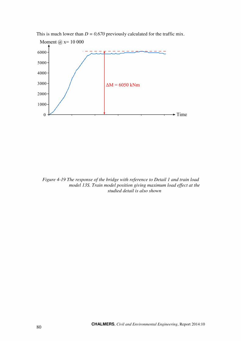
CHALMERS, Civil and Environmental Engineering, Report 2014:10 80
This is much lower than D = 0,670 previously calculated for the traffic mix.
Figure 4-19 The response of the bridge with reference to Detail 1 and train load model 13S. Train model position giving maximum load effect at the
studied detail is also shown
CHALMERS, Civil and Environmental Engineering, Report 2014: 81
5 Fatigue design using the structural hot-spot stress
method
5.1 Introduction
The structural hot-spot stress method has been developed to enable evaluating the fatigue strength of welded structures in cases where the nominal stress is hard to estimate because of geometric and/or loading complexities. This method has been used in the fatigue design of pressure vessels and welded tubular structures since 1960s. The method was later on transferred to non-tubular welded joints in ships and FPSOs (Floating Production, Storage and Offloading units) [12-14] and has finally become a codified procedure for evaluating the fatigue life of welded structures. The philosophy of the structural hot-spot stress method is base the fatigue verification on the structural/geometric stress at the point of crack initiation (usually a weld toe), the so called hot-spot points3. The calculated stress will, thus, include the geometrical stress concentrations generated by the geometry of the detail, as well as any local load redistribution effects, such as those caused by shear lag or warping.
The major advantage of the structural hot-spot stress approach is that the “global” stress raising effects caused by the geometry of the detail are implicitly taken into account in the stress calculations. One consequence of this is that the number of S–N curves needed for fatigue evaluation with the structural hot-spot stress method is substantially reduced, which is another advantage of this method.
An illustrative example that explains the principle difference between the conventional nominal stress method and the structural hot-spot method is shown in Figure 5-1. While six different detail categories are needed to describe the fatigue strength of a simple non-load carrying attachment, based on different geometrical parameters, only one fatigue category is needed when the structural hot-spot stress method is applied. The effect of the stress concentration caused by the geometry of the detail is – in the case of the structural hot-spot stress method – accounted for on the load-effect side, while in the nominal stress method this effect is covered on the resistance side (by assigning different fatigue categories).
3 These points also called reference points, i.e. the critical points in the vicinity of the weld toe; the hot-spots points.
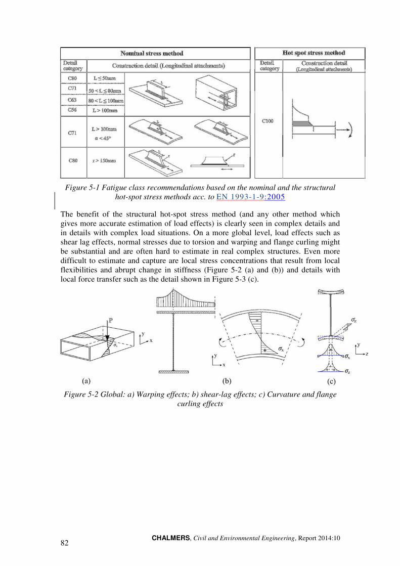
CHALMERS, Civil and Environmental Engineering, Report 2014:10 82
Figure 5-1 Fatigue class recommendations based on the nominal and the structural hot-spot stress methods acc. to EN 1993-1-9:2005
The benefit of the structural hot-spot stress method (and any other method which gives more accurate estimation of load effects) is clearly seen in complex details and in details with complex load situations. On a more global level, load effects such as shear lag effects, normal stresses due to torsion and warping and flange curling might be substantial and are often hard to estimate in real complex structures. Even more difficult to estimate and capture are local stress concentrations that result from local flexibilities and abrupt change in stiffness (Figure 5-2 (a) and (b)) and details with local force transfer such as the detail shown in Figure 5-3 (c).
Figure 5-2 Global: a) Warping effects; b) shear-lag effects; c) Curvature and flange curling effects
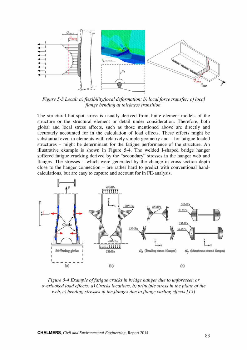
CHALMERS, Civil and Environmental Engineering, Report 2014: 83
Figure 5-3 Local: a) flexibility/local deformation; b) local force transfer; c) local flange bending at thickness transition.
The structural hot-spot stress is usually derived from finite element models of the structure or the structural element or detail under consideration. Therefore, both global and local stress affects, such as those mentioned above are directly and accurately accounted for in the calculation of load effects. These effects might be substantial even in elements with relatively simple geometry and – for fatigue loaded structures – might be determinant for the fatigue performance of the structure. An illustrative example is shown in Figure 5-4. The welded I-shaped bridge hanger suffered fatigue cracking derived by the “secondary” stresses in the hanger web and flanges. The stresses – which were generated by the change in cross-section depth close to the hanger connection – are rather hard to predict with conventional hand-calculations, but are easy to capture and account for in FE-analysis.
Figure 5-4 Example of fatigue cracks in bridge hanger due to unforeseen or overlooked load effects: a) Cracks locations, b) principle stress in the plane of the
web, c) bending stresses in the flanges due to flange curling effects [15]
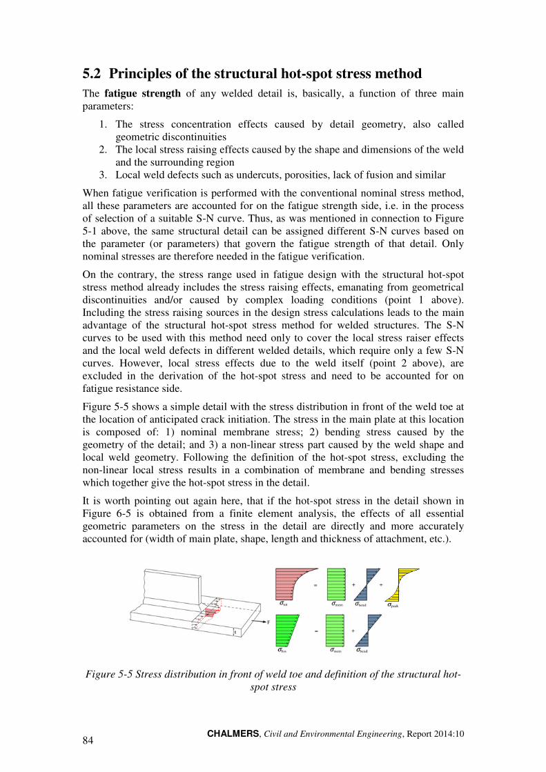
CHALMERS, Civil and Environmental Engineering, Report 2014:10 84
5.2 Principles of the structural hot-spot stress method
The fatigue strength of any welded detail is, basically, a function of three main parameters:
1. The stress concentration effects caused by detail geometry, also called geometric discontinuities
2. The local stress raising effects caused by the shape and dimensions of the weld and the surrounding region
3. Local weld defects such as undercuts, porosities, lack of fusion and similar
When fatigue verification is performed with the conventional nominal stress method, all these parameters are accounted for on the fatigue strength side, i.e. in the process of selection of a suitable S-N curve. Thus, as was mentioned in connection to Figure 5-1 above, the same structural detail can be assigned different S-N curves based on the parameter (or parameters) that govern the fatigue strength of that detail. Only nominal stresses are therefore needed in the fatigue verification.
On the contrary, the stress range used in fatigue design with the structural hot-spot stress method already includes the stress raising effects, emanating from geometrical discontinuities and/or caused by complex loading conditions (point 1 above). Including the stress raising sources in the design stress calculations leads to the main advantage of the structural hot-spot stress method for welded structures. The S-N curves to be used with this method need only to cover the local stress raiser effects and the local weld defects in different welded details, which require only a few S-N curves. However, local stress effects due to the weld itself (point 2 above), are excluded in the derivation of the hot-spot stress and need to be accounted for on fatigue resistance side.
Figure 5-5 shows a simple detail with the stress distribution in front of the weld toe at the location of anticipated crack initiation. The stress in the main plate at this location is composed of: 1) nominal membrane stress; 2) bending stress caused by the geometry of the detail; and 3) a non-linear stress part caused by the weld shape and local weld geometry. Following the definition of the hot-spot stress, excluding the non-linear local stress results in a combination of membrane and bending stresses which together give the hot-spot stress in the detail.
It is worth pointing out again here, that if the hot-spot stress in the detail shown in Figure 6-5 is obtained from a finite element analysis, the effects of all essential geometric parameters on the stress in the detail are directly and more accurately accounted for (width of main plate, shape, length and thickness of attachment, etc.).
Figure 5-5 Stress distribution in front of weld toe and definition of the structural hot-spot stress
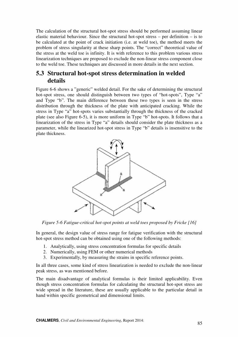
CHALMERS, Civil and Environmental Engineering, Report 2014: 85
The calculation of the structural hot-spot stress should be performed assuming linear elastic material behaviour. Since the structural hot-spot stress – per definition – is to be calculated at the point of crack initiation (i.e. at weld toe), the method meets the problem of stress singularity at these sharp points. The “correct” theoretical value of the stress at the weld toe is infinity. It is with reference to this problem various stress linearization techniques are proposed to exclude the non-linear stress component close to the weld toe. These techniques are discussed in more details in the next section.
5.3 Structural hot-spot stress determination in welded
details
Figure 6-6 shows a ”generic” welded detail. For the sake of determining the structural hot-spot stress, one should distinguish between two types of “hot-spots”, Type “a” and Type “b”. The main difference between these two types is seen in the stress distribution through the thickness of the plate with anticipated cracking. While the stress in Type “a” hot-spots varies substantially through the thickness of the cracked plate (see also Figure 6-5), it is more uniform in Type “b” hot-spots. It follows that a linearization of the stress in Type “a” details should consider the plate thickness as a parameter, while the linearized hot-spot stress in Type “b” details is insensitive to the plate thickness.
Figure 5-6 Fatigue-critical hot-spot points at weld toes proposed by Fricke [16]
In general, the design value of stress range for fatigue verification with the structural hot-spot stress method can be obtained using one of the following methods:
1. Analytically, using stress concentration formulas for specific details 2. Numerically, using FEM or other numerical methods 3. Experimentally, by measuring the strains in specific reference points.
In all three cases, some kind of stress linearization is needed to exclude the non-linear peak stress, as was mentioned before.
The main disadvantage of analytical formulas is their limited applicability. Even though stress concentration formulas for calculating the structural hot-spot stress are wide spread in the literature, these are usually applicable to the particular detail in hand within specific geometrical and dimensional limits.
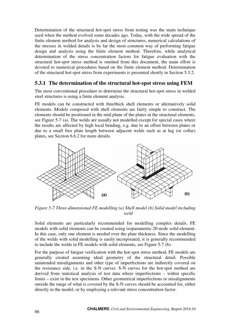
CHALMERS, Civil and Environmental Engineering, Report 2014:10 86
Determination of the structural hot-spot stress from testing was the main technique used when the method evolved some decades ago. Today, with the wide spread of the finite element method for analysis and design of structures, numerical calculations of the stresses in welded details is by far the most common way of performing fatigue design and analysis using the finite element method. Therefore, while analytical determination of the stress concentration factors for fatigue evaluation with the structural hot-spot stress method is omitted from this document, the main effort is devoted to numerical procedures based on the finite element method. Determination of the structural hot-spot stress from experiments is presented shortly in Section 5.3.2.
5.3.1 The determination of the structural hot-spot stress using FEM
The most conventional procedure to determine the structural hot-spot stress in welded steel structures is using a finite element analysis.
FE models can be constructed with thin/thick shell elements or alternatively solid elements. Models composed with shell elements are fairly simple to construct. The elements should be positioned in the mid-plane of the plates in the structural elements, see Figure 5-7 (a). The welds are usually not modelled except for special cases where the results are affected by high local bending, e.g. due to an offset between plates or due to a small free plate length between adjacent welds such as at lug (or collar) plates, see Section 6.6.2 for more details.
Figure 5-7 Three-dimensional FE modelling (a) Shell model (b) Solid model including weld
Solid elements are particularly recommended for modelling complex details. FE models with solid elements can be created using isoparametric 20-node solid element. In this case, only one element is needed over the plate thickness. Since the modelling of the welds with solid modelling is easily incorporated, it is generally recommended to include the welds in FE models with solid elements, see Figure 5-7 (b).
For the purpose of fatigue verification with the hot-spot stress method, FE models are generally created assuming ideal geometry of the structural detail. Possible unintended misalignments and other type of imperfections are indirectly covered on the resistance side, i.e. in the S-N curves. S-N curves for the hot-spot method are derived from statistical analysis of test data where imperfections – within specific limits – exist in the test specimens. Other geometrical imperfections or misalignments outside the range of what is covered by the S-N curves should be accounted for, either directly in the model, or by employing a relevant stress concentration factor.
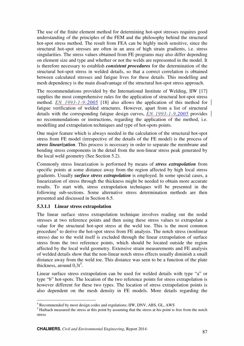
CHALMERS, Civil and Environmental Engineering, Report 2014: 87
The use of the finite element method for determining hot-spot stresses requires good understanding of the principles of the FEM and the philosophy behind the structural hot-spot stress method. The result from FEA can be highly mesh sensitive, since the structural hot-spot stresses are often in an area of high strain gradients, i.e. stress singularities. The stress values obtained from FE programs may also differ depending on element size and type and whether or not the welds are represented in the model. It is therefore necessary to establish consistent procedures for the determination of the structural hot-spot stress in welded details, so that a correct correlation is obtained between calculated stresses and fatigue lives for these details. This modelling and mesh dependency is the main disadvantage of the structural hot-spot stress approach.
The recommendations provided by the International Institute of Welding, IIW [17] supplies the most comprehensive rules for the application of structural hot-spot stress method. EN 1993-1-9:2005 [18] also allows the application of this method for fatigue verification of welded structures. However, apart from a list of structural details with the corresponding fatigue design curves, EN 1993-1-9.2005 provides no recommendations or instructions, regarding the application of the method, i.e. modelling and extrapolation techniques and type of hot-spots points.
One major feature which is always needed in the calculation of the structural hot-spot stress from FE model (irrespective of the details of the FE model) is the process of stress linearization. This process is necessary in order to separate the membrane and bending stress components in the detail from the non-linear stress peak generated by the local weld geometry (See Section 5.2).
Commonly stress linearization is performed by means of stress extrapolation from specific points at some distance away from the region affected by high local stress gradients. Usually surface stress extrapolation is employed. In some special cases, a linearization of stress through the thickness might be needed to obtain more accurate results. To start with, stress extrapolation techniques will be presented in the following sub-sections. Some alternative stress determination methods are then presented and discussed in Section 6.5.
5.3.1.1 Linear stress extrapolation
The linear surface stress extrapolation technique involves reading out the nodal stresses at two reference points and then using these stress values to extrapolate a value for the structural hot-spot stress at the weld toe. This is the most common procedure4 to derive the hot-spot stress from FE analysis. The notch stress (nonlinear stress) due to the weld itself is excluded through the linear extrapolation of surface stress from the two reference points, which should be located outside the region affected by the local weld geometry. Extensive strain measurements and FE analysis of welded details show that the non-linear notch stress effects usually diminish a small distance away from the weld toe. This distance was seen to be a function of the plate thickness, around 0,3t5.
Linear surface stress extrapolation can be used for welded details with type “a” or type “b” hot-spots. The location of the two reference points for stress extrapolation is however different for these two types. The location of stress extrapolation points is also dependent on the mesh density in FE models. More details regarding the
4 Recommended by most design codes and regulations; IIW, DNV, ABS, GL, AWS 5 Haibach measured the stress at this point by assuming that the stress at his point is free from the notch stress
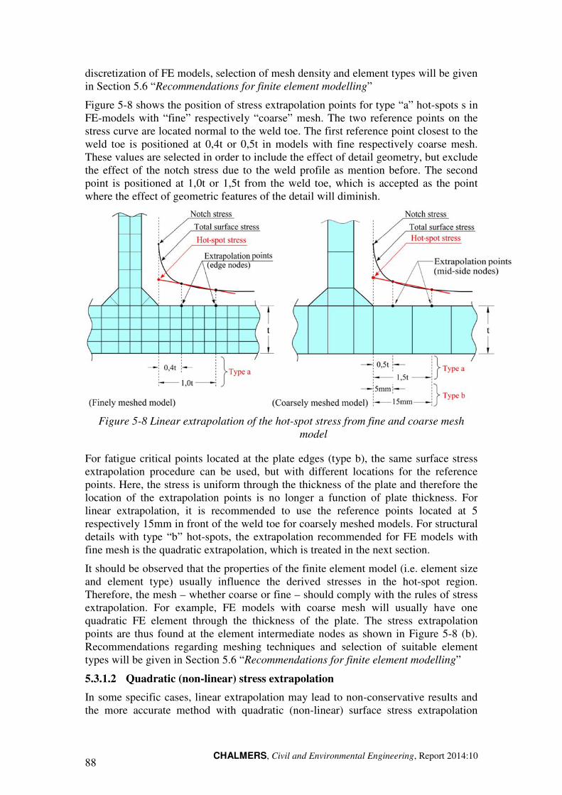
CHALMERS, Civil and Environmental Engineering, Report 2014:10 88
discretization of FE models, selection of mesh density and element types will be given in Section 5.6 “Recommendations for finite element modelling”
Figure 5-8 shows the position of stress extrapolation points for type “a” hot-spots s in FE-models with “fine” respectively “coarse” mesh. The two reference points on the stress curve are located normal to the weld toe. The first reference point closest to the weld toe is positioned at 0,4t or 0,5t in models with fine respectively coarse mesh. These values are selected in order to include the effect of detail geometry, but exclude the effect of the notch stress due to the weld profile as mention before. The second point is positioned at 1,0t or 1,5t from the weld toe, which is accepted as the point where the effect of geometric features of the detail will diminish.
Figure 5-8 Linear extrapolation of the hot-spot stress from fine and coarse mesh model
For fatigue critical points located at the plate edges (type b), the same surface stress extrapolation procedure can be used, but with different locations for the reference points. Here, the stress is uniform through the thickness of the plate and therefore the location of the extrapolation points is no longer a function of plate thickness. For linear extrapolation, it is recommended to use the reference points located at 5 respectively 15mm in front of the weld toe for coarsely meshed models. For structural details with type “b” hot-spots, the extrapolation recommended for FE models with fine mesh is the quadratic extrapolation, which is treated in the next section.
It should be observed that the properties of the finite element model (i.e. element size and element type) usually influence the derived stresses in the hot-spot region. Therefore, the mesh – whether coarse or fine – should comply with the rules of stress extrapolation. For example, FE models with coarse mesh will usually have one quadratic FE element through the thickness of the plate. The stress extrapolation points are thus found at the element intermediate nodes as shown in Figure 5-8 (b). Recommendations regarding meshing techniques and selection of suitable element types will be given in Section 5.6 “Recommendations for finite element modelling”
5.3.1.2 Quadratic (non-linear) stress extrapolation
In some specific cases, linear extrapolation may lead to non-conservative results and the more accurate method with quadratic (non-linear) surface stress extrapolation
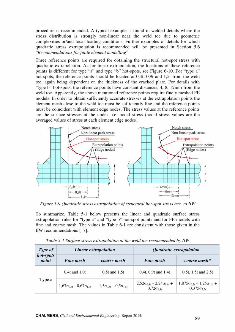
CHALMERS, Civil and Environmental Engineering, Report 2014: 89
procedure is recommended. A typical example is found in welded details where the stress distribution is strongly non-linear near the weld toe due to geometric complexities or/and local loading conditions. Further examples of details for which quadratic stress extrapolation is recommended will be presented in Section 5.6 “Recommendations for finite element modelling”
Three reference points are required for obtaining the structural hot-spot stress with quadratic extrapolation. As for linear extrapolation, the locations of these reference points is different for type “a” and type “b” hot-spots, see Figure 6-10. For “type a” hot-spots, the reference points should be located at 0,4t, 0,9t and 1,5t from the weld toe, again being dependent on the thickness of the cracked plate. For details with “type b” hot-spots, the reference points have constant distances; 4, 8, 12mm from the weld toe. Apparently, the above mentioned reference points require finely meshed FE models. In order to obtain sufficiently accurate stresses at the extrapolation points the element mesh close to the weld toe must be sufficiently fine and the reference points must be coincident with element edge nodes. The stress values at the reference points are the surface stresses at the nodes, i.e. nodal stress (nodal stress values are the averaged values of stress at each element edge nodes).
Figure 5-9 Quadratic stress extrapolation of structural hot-spot stress acc. to IIW
To summarize, Table 5-1 below presents the linear and quadratic surface stress extrapolation rules for “type a” and “type b” hot-spot points and for FE models with fine and coarse mesh. The values in Table 6-1 are consistent with those given in the IIW recommendations [17].
Table 5-1 Surface stress extrapolation at the weld toe recommended by IIW
Type of hot-spots
point
Linear extrapolation Quadratic extrapolation
Fine mesh coarse mesh Fine mesh coarse mesh*
Type a
0,4t and 1,0t 0,5t and 1,5t 0,4t, 0,9t and 1,4t 0,5t, 1,5t and 2,5t
1,67σ0,4t – 0,67σ1,0t 1,5σ0,5t – 0,5σ1.5t 2,52σ0,4t – 2,24σ0,9t +
0,72σ1,4t 1,875σ0,5t – 1,25σ1,5t +
0,375σ2,5t
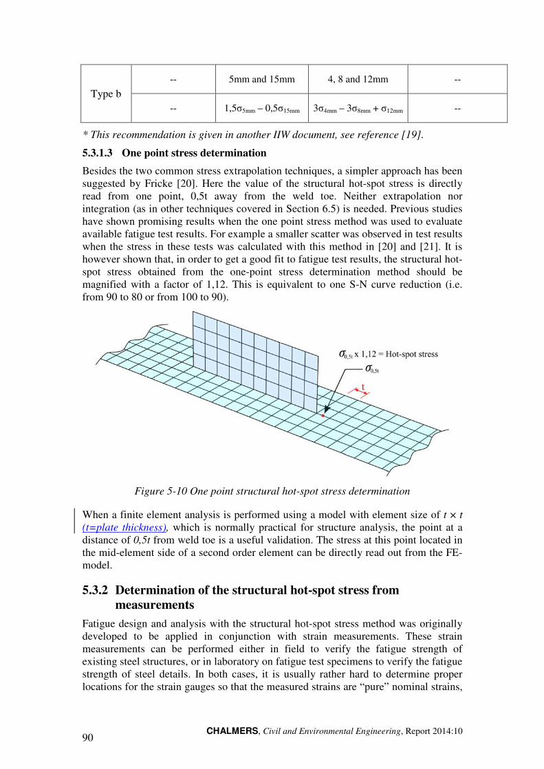
CHALMERS, Civil and Environmental Engineering, Report 2014:10 90
Type b -- 5mm and 15mm 4, 8 and 12mm --
-- 1,5σ5mm – 0,5σ15mm 3σ4mm – 3σ8mm + σ12mm --
* This recommendation is given in another IIW document, see reference [19].
5.3.1.3 One point stress determination
Besides the two common stress extrapolation techniques, a simpler approach has been suggested by Fricke [20]. Here the value of the structural hot-spot stress is directly read from one point, 0,5t away from the weld toe. Neither extrapolation nor integration (as in other techniques covered in Section 6.5) is needed. Previous studies have shown promising results when the one point stress method was used to evaluate available fatigue test results. For example a smaller scatter was observed in test results when the stress in these tests was calculated with this method in [20] and [21]. It is however shown that, in order to get a good fit to fatigue test results, the structural hot-spot stress obtained from the one-point stress determination method should be magnified with a factor of 1,12. This is equivalent to one S-N curve reduction (i.e. from 90 to 80 or from 100 to 90).
Figure 5-10 One point structural hot-spot stress determination
When a finite element analysis is performed using a model with element size of t × t (t=plate thickness), which is normally practical for structure analysis, the point at a distance of 0,5t from weld toe is a useful validation. The stress at this point located in the mid-element side of a second order element can be directly read out from the FE-model.
5.3.2 Determination of the structural hot-spot stress from
measurements
Fatigue design and analysis with the structural hot-spot stress method was originally developed to be applied in conjunction with strain measurements. These strain measurements can be performed either in field to verify the fatigue strength of existing steel structures, or in laboratory on fatigue test specimens to verify the fatigue strength of steel details. In both cases, it is usually rather hard to determine proper locations for the strain gauges so that the measured strains are “pure” nominal strains,
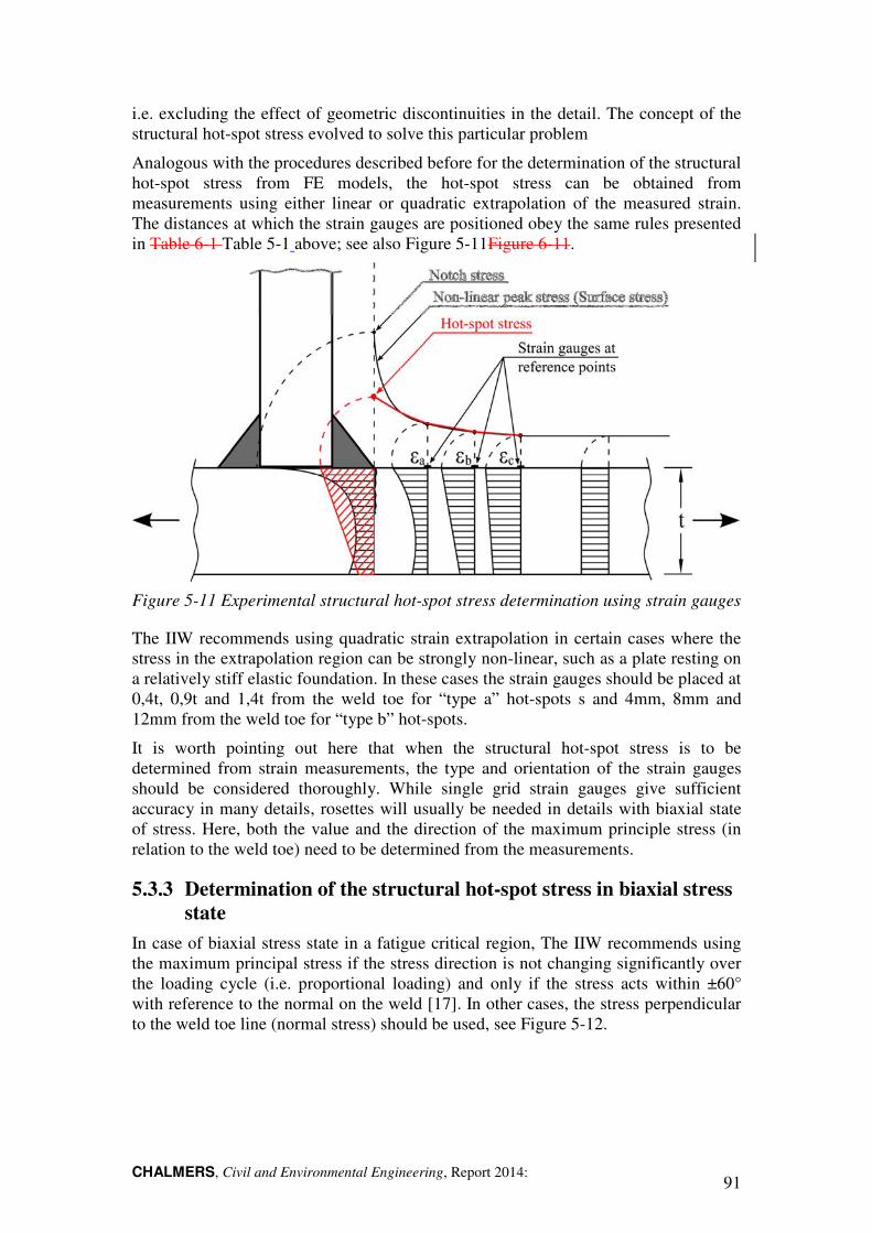
CHALMERS, Civil and Environmental Engineering, Report 2014: 91
i.e. excluding the effect of geometric discontinuities in the detail. The concept of the structural hot-spot stress evolved to solve this particular problem
Analogous with the procedures described before for the determination of the structural hot-spot stress from FE models, the hot-spot stress can be obtained from measurements using either linear or quadratic extrapolation of the measured strain. The distances at which the strain gauges are positioned obey the same rules presented in Table 6-1 Table 5-1 above; see also Figure 5-11Figure 6-11.
Figure 5-11 Experimental structural hot-spot stress determination using strain gauges
The IIW recommends using quadratic strain extrapolation in certain cases where the stress in the extrapolation region can be strongly non-linear, such as a plate resting on a relatively stiff elastic foundation. In these cases the strain gauges should be placed at 0,4t, 0,9t and 1,4t from the weld toe for “type a” hot-spots s and 4mm, 8mm and 12mm from the weld toe for “type b” hot-spots.
It is worth pointing out here that when the structural hot-spot stress is to be determined from strain measurements, the type and orientation of the strain gauges should be considered thoroughly. While single grid strain gauges give sufficient accuracy in many details, rosettes will usually be needed in details with biaxial state of stress. Here, both the value and the direction of the maximum principle stress (in relation to the weld toe) need to be determined from the measurements.
5.3.3 Determination of the structural hot-spot stress in biaxial stress
state
In case of biaxial stress state in a fatigue critical region, The IIW recommends using the maximum principal stress if the stress direction is not changing significantly over the loading cycle (i.e. proportional loading) and only if the stress acts within ±60° with reference to the normal on the weld [17]. In other cases, the stress perpendicular to the weld toe line (normal stress) should be used, see Figure 5-12.
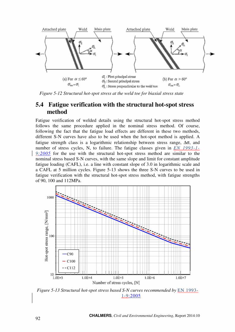
CHALMERS, Civil and Environmental Engineering, Report 2014:10 92
Figure 5-12 Structural hot-spot stress at the weld toe for biaxial stress state
5.4 Fatigue verification with the structural hot-spot stress
method
Fatigue verification of welded details using the structural hot-spot stress method follows the same procedure applied in the nominal stress method. Of course, following the fact that the fatigue load effects are different in these two methods, different S-N curves have also to be used when the hot-spot method is applied. A fatigue strength class is a logarithmic relationship between stress range, ∆σ, and number of stress cycles, N, to failure. The fatigue classes given in EN 1993-1-9:2005 for the use with the structural hot-spot stress method are similar to the nominal stress based S-N curves, with the same slope and limit for constant amplitude fatigue loading (CAFL), i.e. a line with constant slope of 3.0 in logarithmic scale and a CAFL at 5 million cycles. Figure 5-13 shows the three S-N curves to be used in fatigue verification with the structural hot-spot stress method, with fatigue strengths of 90, 100 and 112MPa.
Figure 5-13 Structural hot-spot stress based S-N curves recommended by EN 1993-1-9:2005
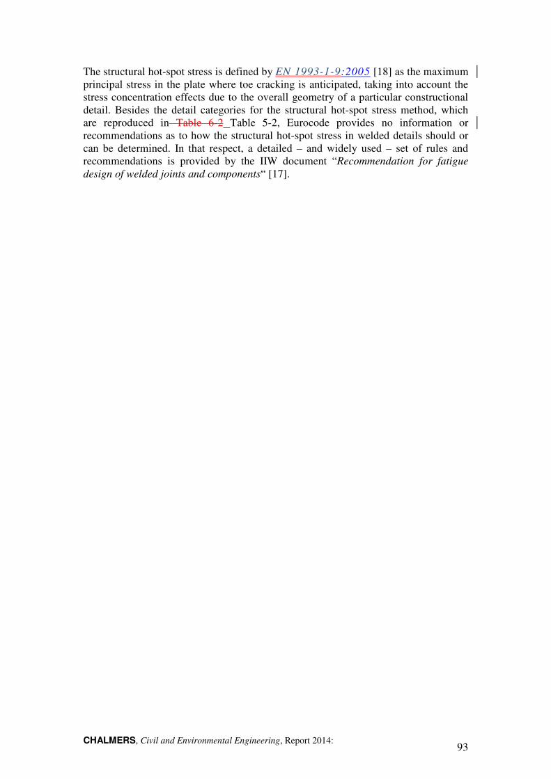
CHALMERS, Civil and Environmental Engineering, Report 2014: 93
The structural hot-spot stress is defined by EN 1993-1-9:2005 [18] as the maximum principal stress in the plate where toe cracking is anticipated, taking into account the stress concentration effects due to the overall geometry of a particular constructional detail. Besides the detail categories for the structural hot-spot stress method, which are reproduced in Table 6-2 Table 5-2, Eurocode provides no information or recommendations as to how the structural hot-spot stress in welded details should or can be determined. In that respect, a detailed – and widely used – set of rules and recommendations is provided by the IIW document “Recommendation for fatigue design of welded joints and components“ [17].
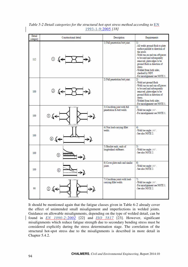
CHALMERS, Civil and Environmental Engineering, Report 2014:10 94
Table 5-2 Detail categories for the structural hot-spot stress method according to EN 1993-1-9:2005 [18]
It should be mentioned again that the fatigue classes given in Table 6-2 already cover the effect of unintended small misalignment and imperfections in welded joints. Guidance on allowable misalignments, depending on the type of welded detail, can be found in EN 1090-2:2002 [22] and ISO 5817 [23]. However, significant misalignments which reduce fatigue strength due to secondary bending stress must be considered explicitly during the stress determination stage. The correlation of the structural hot-spot stress due to the misalignments is described in more detail in Chapter 5.4.2.
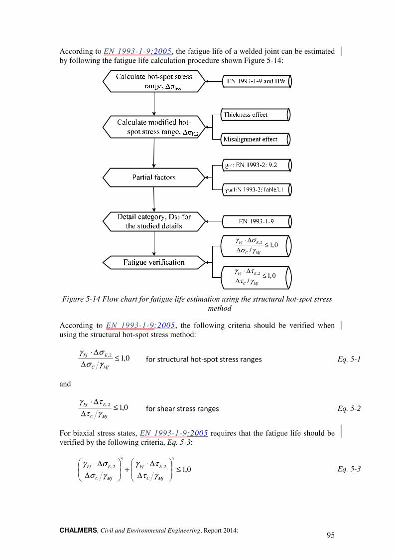
CHALMERS, Civil and Environmental Engineering, Report 2014: 95
According to EN 1993-1-9:2005, the fatigue life of a welded joint can be estimated by following the fatigue life calculation procedure shown Figure 5-14:
,2 1,0/
Ff E
C Mf
γ σ
σ γ
⋅ ∆≤
∆
,2 1,0/
Ff E
C Mf
γ τ
τ γ
⋅ ∆≤
∆
Figure 5-14 Flow chart for fatigue life estimation using the structural hot-spot stress method
According to EN 1993-1-9:2005, the following criteria should be verified when using the structural hot-spot stress method:
0,12,≤
∆
∆⋅
MfC
EFf
γσ
σγ
for structural hot-spot stress ranges Eq. 5-1
and
0,12,≤
∆
∆⋅
MfC
EFf
γτ
τγ
for shear stress ranges Eq. 5-2
For biaxial stress states, EN 1993-1-9:2005 requires that the fatigue life should be verified by the following criteria, Eq. 5-3:
0,1
5
2,
3
2, ≤
∆
∆⋅+
∆
∆⋅
MfC
EFf
MfC
EFf
γτ
τγ
γσ
σγ
Eq. 5-3
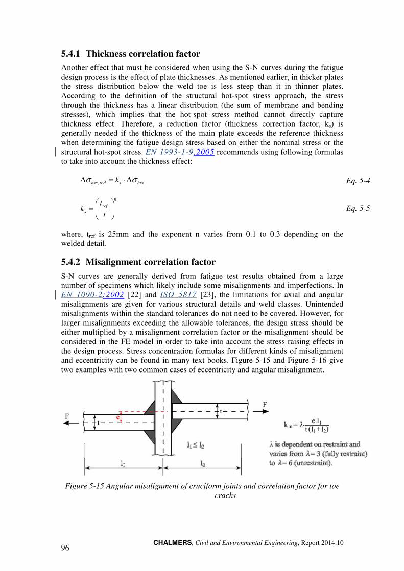
CHALMERS, Civil and Environmental Engineering, Report 2014:10 96
5.4.1 Thickness correlation factor
Another effect that must be considered when using the S-N curves during the fatigue design process is the effect of plate thicknesses. As mentioned earlier, in thicker plates the stress distribution below the weld toe is less steep than it in thinner plates. According to the definition of the structural hot-spot stress approach, the stress through the thickness has a linear distribution (the sum of membrane and bending stresses), which implies that the hot-spot stress method cannot directly capture thickness effect. Therefore, a reduction factor (thickness correction factor, ks) is generally needed if the thickness of the main plate exceeds the reference thickness when determining the fatigue design stress based on either the nominal stress or the structural hot-spot stress. EN 1993-1-9.2005 recommends using following formulas to take into account the thickness effect:
hsssredhss k σσ ∆⋅=∆ , Eq. 5-4
n
refs t
tk
= Eq. 5-5
where, tref is 25mm and the exponent n varies from 0.1 to 0.3 depending on the welded detail.
5.4.2 Misalignment correlation factor
S-N curves are generally derived from fatigue test results obtained from a large number of specimens which likely include some misalignments and imperfections. In EN 1090-2:2002 [22] and ISO 5817 [23], the limitations for axial and angular misalignments are given for various structural details and weld classes. Unintended misalignments within the standard tolerances do not need to be covered. However, for larger misalignments exceeding the allowable tolerances, the design stress should be either multiplied by a misalignment correlation factor or the misalignment should be considered in the FE model in order to take into account the stress raising effects in the design process. Stress concentration formulas for different kinds of misalignment and eccentricity can be found in many text books. Figure 5-15 and Figure 5-16 give two examples with two common cases of eccentricity and angular misalignment.
Figure 5-15 Angular misalignment of cruciform joints and correlation factor for toe cracks
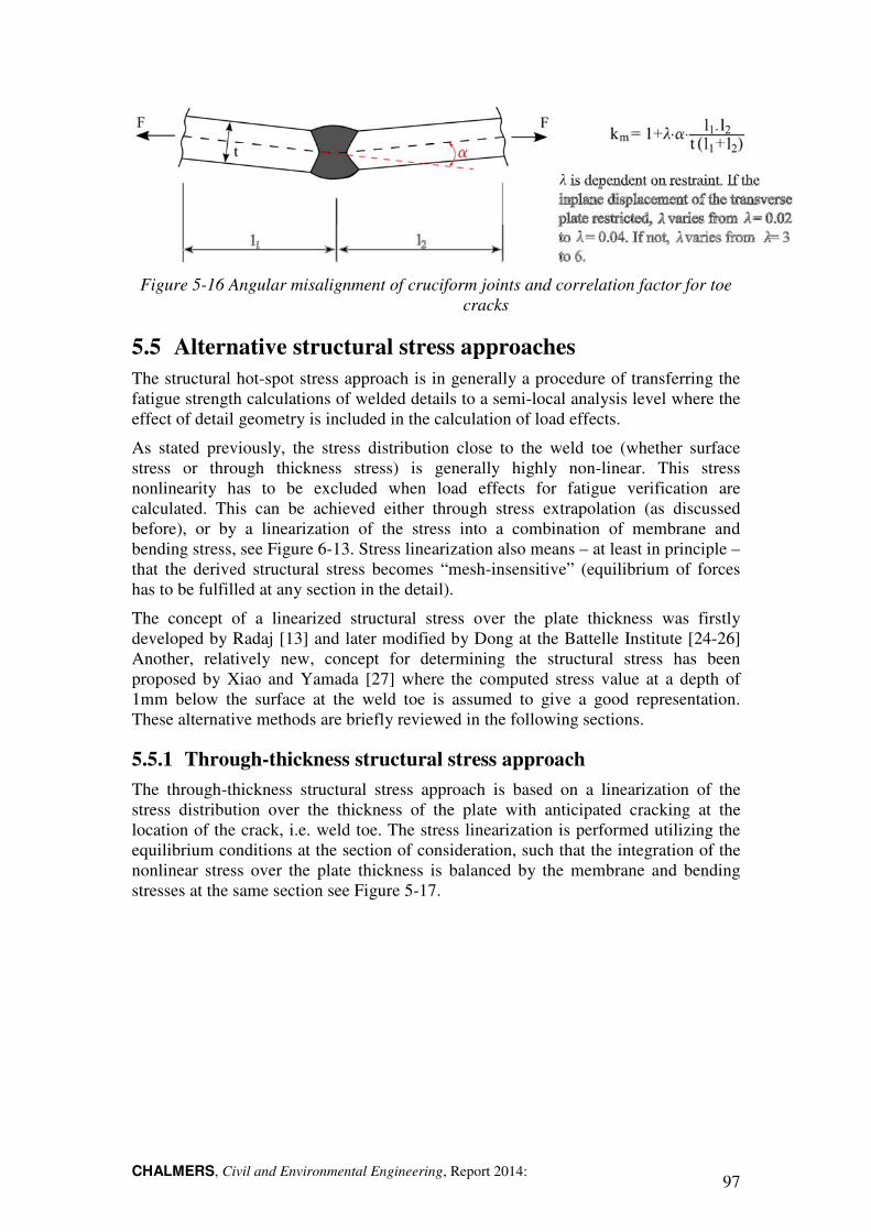
CHALMERS, Civil and Environmental Engineering, Report 2014: 97
Figure 5-16 Angular misalignment of cruciform joints and correlation factor for toe cracks
5.5 Alternative structural stress approaches
The structural hot-spot stress approach is in generally a procedure of transferring the fatigue strength calculations of welded details to a semi-local analysis level where the effect of detail geometry is included in the calculation of load effects.
As stated previously, the stress distribution close to the weld toe (whether surface stress or through thickness stress) is generally highly non-linear. This stress nonlinearity has to be excluded when load effects for fatigue verification are calculated. This can be achieved either through stress extrapolation (as discussed before), or by a linearization of the stress into a combination of membrane and bending stress, see Figure 6-13. Stress linearization also means – at least in principle – that the derived structural stress becomes “mesh-insensitive” (equilibrium of forces has to be fulfilled at any section in the detail).
The concept of a linearized structural stress over the plate thickness was firstly developed by Radaj [13] and later modified by Dong at the Battelle Institute [24-26] Another, relatively new, concept for determining the structural stress has been proposed by Xiao and Yamada [27] where the computed stress value at a depth of 1mm below the surface at the weld toe is assumed to give a good representation. These alternative methods are briefly reviewed in the following sections.
5.5.1 Through-thickness structural stress approach
The through-thickness structural stress approach is based on a linearization of the stress distribution over the thickness of the plate with anticipated cracking at the location of the crack, i.e. weld toe. The stress linearization is performed utilizing the equilibrium conditions at the section of consideration, such that the integration of the nonlinear stress over the plate thickness is balanced by the membrane and bending stresses at the same section see Figure 5-17.
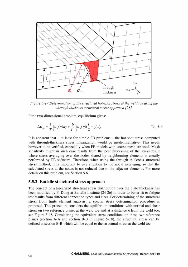
CHALMERS, Civil and Environmental Engineering, Report 2014:10 98
Figure 5-17 Determination of the structural hot-spot stress at the weld toe using the through thickness structural stress approach [28]
For a two-dimensional problem, equilibrium gives:
∫ −+∫=∆T
x
T
xstr dyyT
yT
dyyT 0
20
)2
)((6
)(1
σσσ Eq. 5-6
It is apparent that – at least for simple 2D-problems – the hot-spot stress computed with through-thickness stress linearization would be mesh-insensitive. This needs however to be verified, especially when FE models with coarse mesh are used. Mesh sensitivity might in such case results from the post processing of the stress result where stress averaging over the nodes shared by neighbouring elements is usually performed by FE software. Therefore, when using the through thickness structural stress method, it is important to pay attention to the nodal averaging, so that the calculated stress at the nodes is not reduced due to the adjacent elements. For more details on this problem, see Section 5.6.
5.5.2 Battelle structural stress approach
The concept of a linearized structural stress distribution over the plate thickness has been modified by P. Dong at Battelle Institute [24-26] in order to better fit to fatigue test results from different connection types and sizes. For determining of the structural stress from finite element analysis, a special stress determination procedure is proposed. This procedure considers the equilibrium conditions with normal and shear stress on two reference plane, at the weld toe and at a distance δ from the weld toe, see Figure 5-18. Considering the equivalent stress conditions on these two reference planes (section A-A and section B-B in Figure 5-18), the structural stress can be defined at section B-B which will be equal to the structural stress at the weld toe.
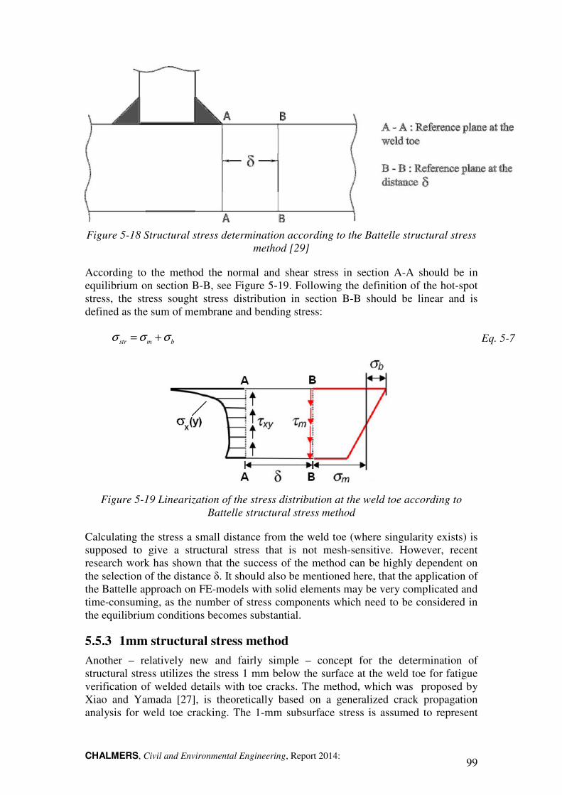
CHALMERS, Civil and Environmental Engineering, Report 2014: 99
Figure 5-18 Structural stress determination according to the Battelle structural stress method [29]
According to the method the normal and shear stress in section A-A should be in equilibrium on section B-B, see Figure 5-19. Following the definition of the hot-spot stress, the stress sought stress distribution in section B-B should be linear and is defined as the sum of membrane and bending stress:
bmstr σσσ += Eq. 5-7
Figure 5-19 Linearization of the stress distribution at the weld toe according to Battelle structural stress method
Calculating the stress a small distance from the weld toe (where singularity exists) is supposed to give a structural stress that is not mesh-sensitive. However, recent research work has shown that the success of the method can be highly dependent on the selection of the distance δ. It should also be mentioned here, that the application of the Battelle approach on FE-models with solid elements may be very complicated and time-consuming, as the number of stress components which need to be considered in the equilibrium conditions becomes substantial.
5.5.3 1mm structural stress method
Another – relatively new and fairly simple – concept for the determination of structural stress utilizes the stress 1 mm below the surface at the weld toe for fatigue verification of welded details with toe cracks. The method, which was proposed by Xiao and Yamada [27], is theoretically based on a generalized crack propagation analysis for weld toe cracking. The 1-mm subsurface stress is assumed to represent
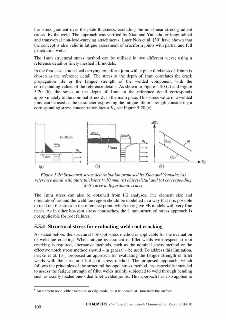
CHALMERS, Civil and Environmental Engineering, Report 2014:10 100
the stress gradient over the plate thickness, excluding the non-linear stress gradient caused by the weld. The approach was verified by Xiao and Yamada for longitudinal and transversal non-load-carrying attachments. Later Noh et al. [30] have shown that the concept is also valid in fatigue assessment of cruciform joints with partial and full penetration welds.
The 1mm structural stress method can be utilized in two different ways; using a reference detail or finely meshed FE models.
In the first case, a non-load carrying cruciform joint with a plate thickness of 10mm is chosen as the reference detail. The stress at the depth of 1mm correlates the crack propagation life or the fatigue strength of the welded component with the corresponding values of the reference details. As shown in Figure 5-20 (a) and Figure 5-20 (b), the stress at the depth of 1mm in the reference detail corresponds approximately to the nominal stress σn in the main plate. This stress value in a welded joint can be used as the parameter expressing the fatigue life or strength considering a corresponding stress concentration factor Ks, see Figure 5-20 (c).
Figure 5-20 Structural stress determination proposed by Xiao and Yamada; (a) reference detail with plate thickness t=10 mm, (b) object detail and (c) corresponding
S–N curve in logarithmic scales
The 1mm stress can also be obtained from FE analyses. The element size and orientation6 around the weld toe region should be modelled in a way that it is possible to read out the stress in the reference point, which may give FE models with very fine mesh. As in other hot-spot stress approaches, the 1 mm structural stress approach is not applicable for root failures.
5.5.4 Structural stress for evaluating weld root cracking
As stated before, the structural hot-spot stress method is applicable for the evaluation of weld toe cracking. When fatigue assessment of fillet welds with respect to root cracking is required, alternative methods, such as the nominal stress method or the effective notch stress method should – in general – be used. To address this limitation, Fricke et al. [31] proposed an approach for evaluating the fatigue strength of fillet welds with the structural hot-spot stress method. The proposed approach, which follows the principles of the structural hot-spot stress method, has especially intended to assess the fatigue strength of fillet welds mainly subjected to weld through bending such as axially loaded one-sided fillet welded joints. This approach has also applied to
6 An element node, either mid-side or edge node, must be located at 1mm from the surface.
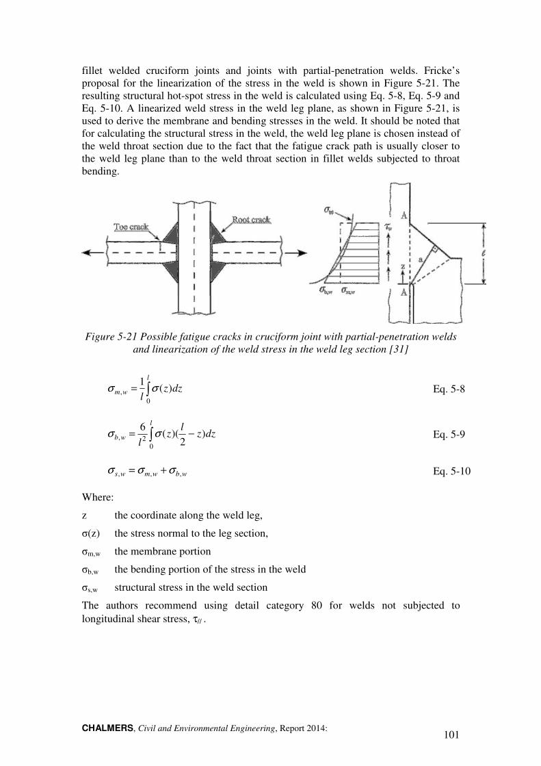
CHALMERS, Civil and Environmental Engineering, Report 2014: 101
fillet welded cruciform joints and joints with partial-penetration welds. Fricke’s proposal for the linearization of the stress in the weld is shown in Figure 5-21. The resulting structural hot-spot stress in the weld is calculated using Eq. 5-8, Eq. 5-9 and Eq. 5-10. A linearized weld stress in the weld leg plane, as shown in Figure 5-21, is used to derive the membrane and bending stresses in the weld. It should be noted that for calculating the structural stress in the weld, the weld leg plane is chosen instead of the weld throat section due to the fact that the fatigue crack path is usually closer to the weld leg plane than to the weld throat section in fillet welds subjected to throat bending.
Figure 5-21 Possible fatigue cracks in cruciform joint with partial-penetration welds and linearization of the weld stress in the weld leg section [31]
∫=l
wm dzzl 0
, )(1
σσ Eq. 5-8
∫ −=l
wb dzzl
zl 0
2, )2
)((6
σσ Eq. 5-9
wbwmws ,,, σσσ += Eq. 5-10
Where:
z the coordinate along the weld leg,
σ(z) the stress normal to the leg section,
σm,w the membrane portion
σb,w the bending portion of the stress in the weld
σs,w structural stress in the weld section
The authors recommend using detail category 80 for welds not subjected to longitudinal shear stress, τ// .
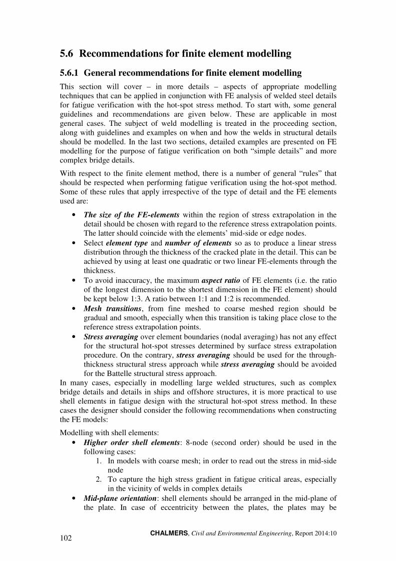
CHALMERS, Civil and Environmental Engineering, Report 2014:10 102
5.6 Recommendations for finite element modelling
5.6.1 General recommendations for finite element modelling
This section will cover – in more details – aspects of appropriate modelling techniques that can be applied in conjunction with FE analysis of welded steel details for fatigue verification with the hot-spot stress method. To start with, some general guidelines and recommendations are given below. These are applicable in most general cases. The subject of weld modelling is treated in the proceeding section, along with guidelines and examples on when and how the welds in structural details should be modelled. In the last two sections, detailed examples are presented on FE modelling for the purpose of fatigue verification on both “simple details” and more complex bridge details.
With respect to the finite element method, there is a number of general “rules” that should be respected when performing fatigue verification using the hot-spot method. Some of these rules that apply irrespective of the type of detail and the FE elements used are:
• The size of the FE-elements within the region of stress extrapolation in the detail should be chosen with regard to the reference stress extrapolation points. The latter should coincide with the elements’ mid-side or edge nodes.
• Select element type and number of elements so as to produce a linear stress distribution through the thickness of the cracked plate in the detail. This can be achieved by using at least one quadratic or two linear FE-elements through the thickness.
• To avoid inaccuracy, the maximum aspect ratio of FE elements (i.e. the ratio of the longest dimension to the shortest dimension in the FE element) should be kept below 1:3. A ratio between 1:1 and 1:2 is recommended.
• Mesh transitions, from fine meshed to coarse meshed region should be gradual and smooth, especially when this transition is taking place close to the reference stress extrapolation points.
• Stress averaging over element boundaries (nodal averaging) has not any effect for the structural hot-spot stresses determined by surface stress extrapolation procedure. On the contrary, stress averaging should be used for the through-thickness structural stress approach while stress averaging should be avoided for the Battelle structural stress approach.
In many cases, especially in modelling large welded structures, such as complex bridge details and details in ships and offshore structures, it is more practical to use shell elements in fatigue design with the structural hot-spot stress method. In these cases the designer should consider the following recommendations when constructing the FE models:
Modelling with shell elements: • Higher order shell elements: 8-node (second order) should be used in the
following cases: 1. In models with coarse mesh; in order to read out the stress in mid-side
node 2. To capture the high stress gradient in fatigue critical areas, especially
in the vicinity of welds in complex details • Mid-plane orientation: shell elements should be arranged in the mid-plane of
the plate. In case of eccentricity between the plates, the plates may be
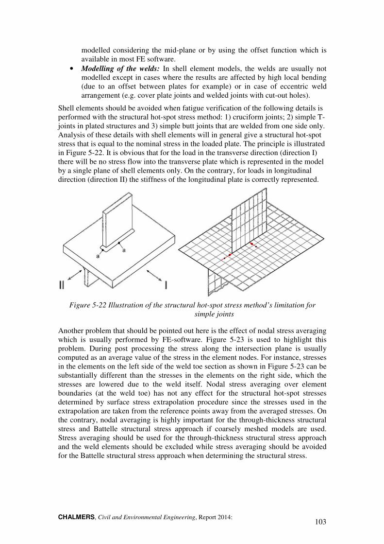
CHALMERS, Civil and Environmental Engineering, Report 2014: 103
modelled considering the mid-plane or by using the offset function which is available in most FE software.
• Modelling of the welds: In shell element models, the welds are usually not modelled except in cases where the results are affected by high local bending (due to an offset between plates for example) or in case of eccentric weld arrangement (e.g. cover plate joints and welded joints with cut-out holes).
Shell elements should be avoided when fatigue verification of the following details is performed with the structural hot-spot stress method: 1) cruciform joints; 2) simple T-joints in plated structures and 3) simple butt joints that are welded from one side only. Analysis of these details with shell elements will in general give a structural hot-spot stress that is equal to the nominal stress in the loaded plate. The principle is illustrated in Figure 5-22. It is obvious that for the load in the transverse direction (direction I) there will be no stress flow into the transverse plate which is represented in the model by a single plane of shell elements only. On the contrary, for loads in longitudinal direction (direction II) the stiffness of the longitudinal plate is correctly represented.
Figure 5-22 Illustration of the structural hot-spot stress method’s limitation for simple joints
Another problem that should be pointed out here is the effect of nodal stress averaging which is usually performed by FE-software. Figure 5-23 is used to highlight this problem. During post processing the stress along the intersection plane is usually computed as an average value of the stress in the element nodes. For instance, stresses in the elements on the left side of the weld toe section as shown in Figure 5-23 can be substantially different than the stresses in the elements on the right side, which the stresses are lowered due to the weld itself. Nodal stress averaging over element boundaries (at the weld toe) has not any effect for the structural hot-spot stresses determined by surface stress extrapolation procedure since the stresses used in the extrapolation are taken from the reference points away from the averaged stresses. On the contrary, nodal averaging is highly important for the through-thickness structural stress and Battelle structural stress approach if coarsely meshed models are used. Stress averaging should be used for the through-thickness structural stress approach and the weld elements should be excluded while stress averaging should be avoided for the Battelle structural stress approach when determining the structural stress.
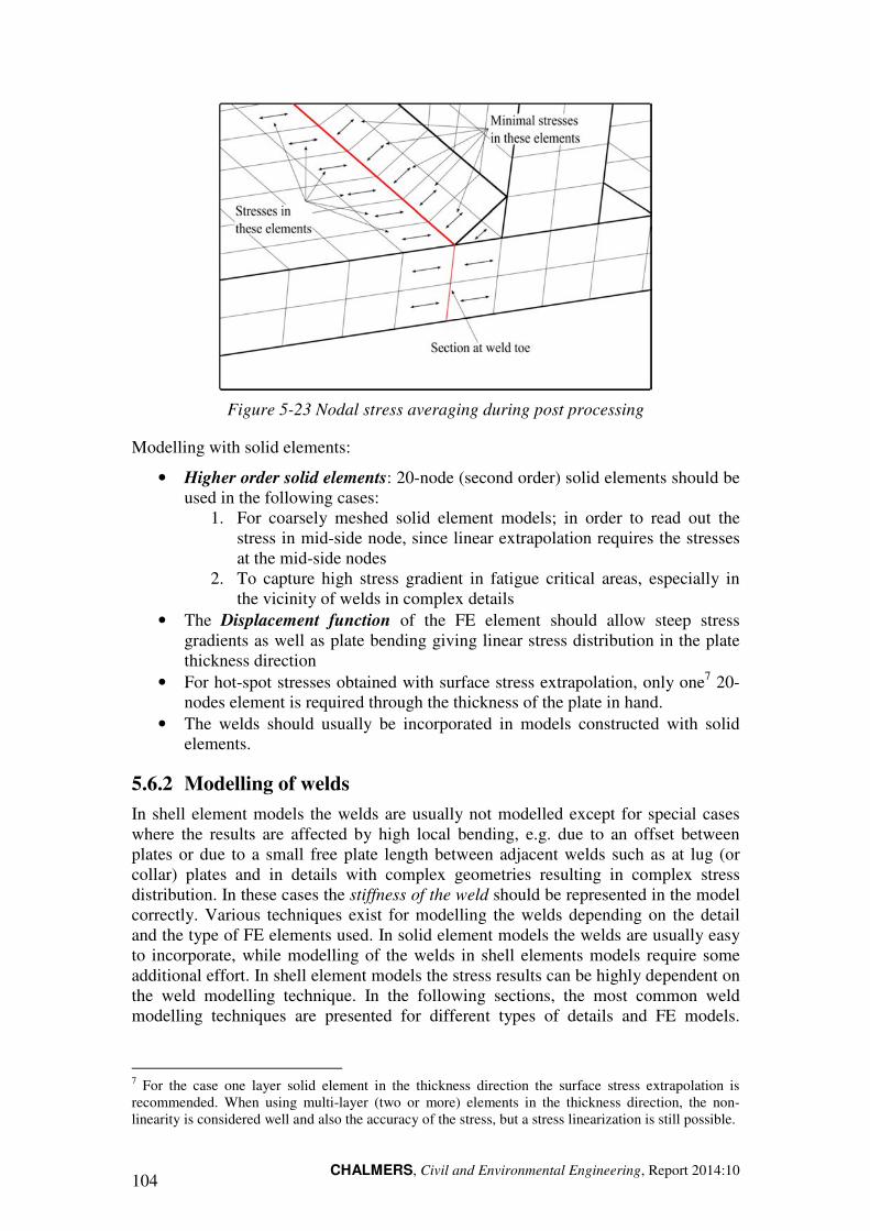
CHALMERS, Civil and Environmental Engineering, Report 2014:10 104
Figure 5-23 Nodal stress averaging during post processing
Modelling with solid elements:
• Higher order solid elements: 20-node (second order) solid elements should be used in the following cases:
1. For coarsely meshed solid element models; in order to read out the stress in mid-side node, since linear extrapolation requires the stresses at the mid-side nodes
2. To capture high stress gradient in fatigue critical areas, especially in the vicinity of welds in complex details
• The Displacement function of the FE element should allow steep stress gradients as well as plate bending giving linear stress distribution in the plate thickness direction
• For hot-spot stresses obtained with surface stress extrapolation, only one7 20-nodes element is required through the thickness of the plate in hand.
• The welds should usually be incorporated in models constructed with solid elements.
5.6.2 Modelling of welds
In shell element models the welds are usually not modelled except for special cases where the results are affected by high local bending, e.g. due to an offset between plates or due to a small free plate length between adjacent welds such as at lug (or collar) plates and in details with complex geometries resulting in complex stress distribution. In these cases the stiffness of the weld should be represented in the model correctly. Various techniques exist for modelling the welds depending on the detail and the type of FE elements used. In solid element models the welds are usually easy to incorporate, while modelling of the welds in shell elements models require some additional effort. In shell element models the stress results can be highly dependent on the weld modelling technique. In the following sections, the most common weld modelling techniques are presented for different types of details and FE models.
7 For the case one layer solid element in the thickness direction the surface stress extrapolation is recommended. When using multi-layer (two or more) elements in the thickness direction, the non-linearity is considered well and also the accuracy of the stress, but a stress linearization is still possible.
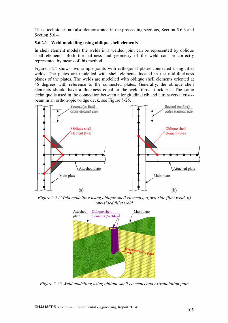
CHALMERS, Civil and Environmental Engineering, Report 2014: 105
These techniques are also demonstrated in the proceeding sections, Section 5.6.3 and Section 5.6.4.
5.6.2.1 Weld modelling using oblique shell elements
In shell element models the welds in a welded joint can be represented by oblique shell elements. Both the stiffness and geometry of the weld can be correctly represented by means of this method.
Figure 5-24 shows two simple joints with orthogonal plates connected using fillet welds. The plates are modelled with shell elements located in the mid-thickness planes of the plates. The welds are modelled with oblique shell elements oriented at 45 degrees with reference to the connected plates. Generally, the oblique shell elements should have a thickness equal to the weld throat thickness. The same technique is used in the connection between a longitudinal rib and a transversal cross-beam in an orthotropic bridge deck, see Figure 5-25.
Figure 5-24 Weld modelling using oblique shell elements; a)two-side fillet weld, b) one-sided fillet weld
Figure 5-25 Weld modelling using oblique shell elements and extrapolation path
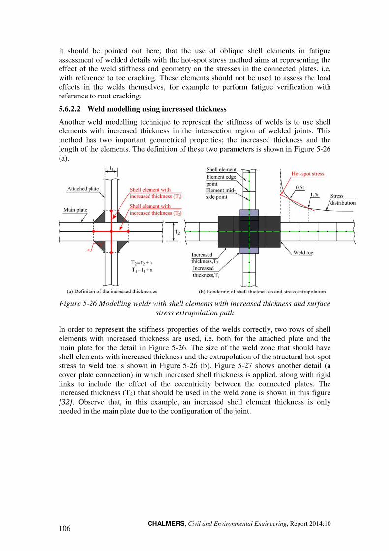
CHALMERS, Civil and Environmental Engineering, Report 2014:10 106
It should be pointed out here, that the use of oblique shell elements in fatigue assessment of welded details with the hot-spot stress method aims at representing the effect of the weld stiffness and geometry on the stresses in the connected plates, i.e. with reference to toe cracking. These elements should not be used to assess the load effects in the welds themselves, for example to perform fatigue verification with reference to root cracking.
5.6.2.2 Weld modelling using increased thickness
Another weld modelling technique to represent the stiffness of welds is to use shell elements with increased thickness in the intersection region of welded joints. This method has two important geometrical properties; the increased thickness and the length of the elements. The definition of these two parameters is shown in Figure 5-26 (a).
Figure 5-26 Modelling welds with shell elements with increased thickness and surface stress extrapolation path
In order to represent the stiffness properties of the welds correctly, two rows of shell elements with increased thickness are used, i.e. both for the attached plate and the main plate for the detail in Figure 5-26. The size of the weld zone that should have shell elements with increased thickness and the extrapolation of the structural hot-spot stress to weld toe is shown in Figure 5-26 (b). Figure 5-27 shows another detail (a cover plate connection) in which increased shell thickness is applied, along with rigid links to include the effect of the eccentricity between the connected plates. The increased thickness (T2) that should be used in the weld zone is shown in this figure [32]. Observe that, in this example, an increased shell element thickness is only needed in the main plate due to the configuration of the joint.
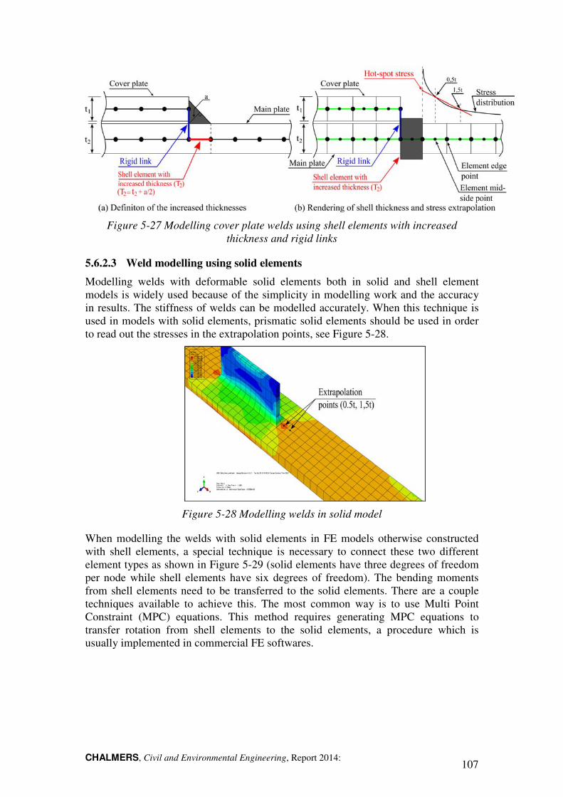
CHALMERS, Civil and Environmental Engineering, Report 2014: 107
Figure 5-27 Modelling cover plate welds using shell elements with increased thickness and rigid links
5.6.2.3 Weld modelling using solid elements
Modelling welds with deformable solid elements both in solid and shell element models is widely used because of the simplicity in modelling work and the accuracy in results. The stiffness of welds can be modelled accurately. When this technique is used in models with solid elements, prismatic solid elements should be used in order to read out the stresses in the extrapolation points, see Figure 5-28.
Figure 5-28 Modelling welds in solid model
When modelling the welds with solid elements in FE models otherwise constructed with shell elements, a special technique is necessary to connect these two different element types as shown in Figure 5-29 (solid elements have three degrees of freedom per node while shell elements have six degrees of freedom). The bending moments from shell elements need to be transferred to the solid elements. There are a couple techniques available to achieve this. The most common way is to use Multi Point Constraint (MPC) equations. This method requires generating MPC equations to transfer rotation from shell elements to the solid elements, a procedure which is usually implemented in commercial FE softwares.
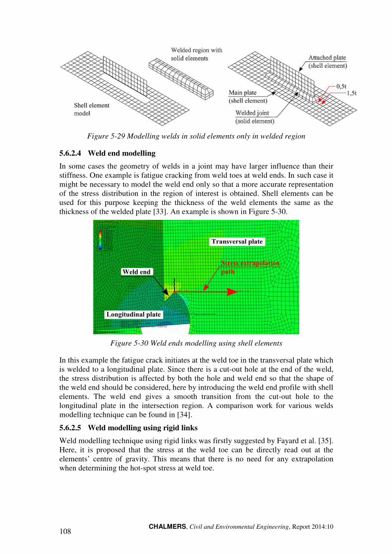
CHALMERS, Civil and Environmental Engineering, Report 2014:10 108
Figure 5-29 Modelling welds in solid elements only in welded region
5.6.2.4 Weld end modelling
In some cases the geometry of welds in a joint may have larger influence than their stiffness. One example is fatigue cracking from weld toes at weld ends. In such case it might be necessary to model the weld end only so that a more accurate representation of the stress distribution in the region of interest is obtained. Shell elements can be used for this purpose keeping the thickness of the weld elements the same as the thickness of the welded plate [33]. An example is shown in Figure 5-30.
Figure 5-30 Weld ends modelling using shell elements
In this example the fatigue crack initiates at the weld toe in the transversal plate which is welded to a longitudinal plate. Since there is a cut-out hole at the end of the weld, the stress distribution is affected by both the hole and weld end so that the shape of the weld end should be considered, here by introducing the weld end profile with shell elements. The weld end gives a smooth transition from the cut-out hole to the longitudinal plate in the intersection region. A comparison work for various welds modelling technique can be found in [34].
5.6.2.5 Weld modelling using rigid links
Weld modelling technique using rigid links was firstly suggested by Fayard et al. [35]. Here, it is proposed that the stress at the weld toe can be directly read out at the elements’ centre of gravity. This means that there is no need for any extrapolation when determining the hot-spot stress at weld toe.
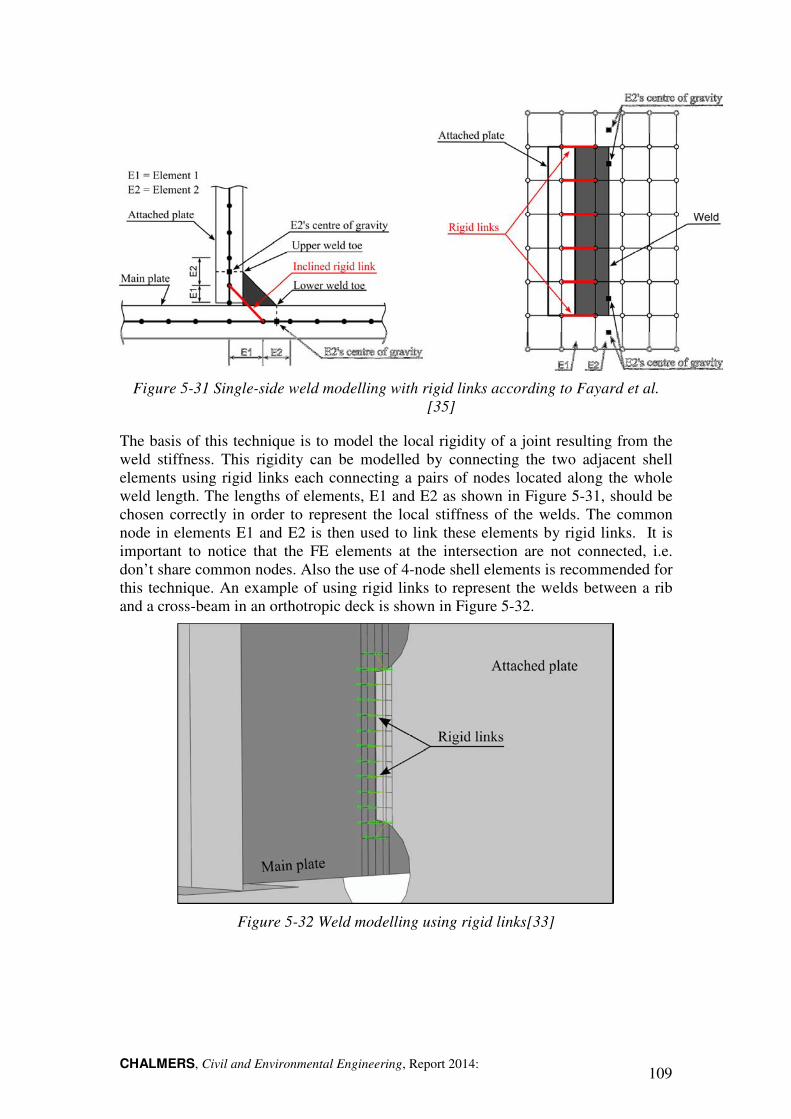
CHALMERS, Civil and Environmental Engineering, Report 2014: 109
Figure 5-31 Single-side weld modelling with rigid links according to Fayard et al. [35]
The basis of this technique is to model the local rigidity of a joint resulting from the weld stiffness. This rigidity can be modelled by connecting the two adjacent shell elements using rigid links each connecting a pairs of nodes located along the whole weld length. The lengths of elements, E1 and E2 as shown in Figure 5-31, should be chosen correctly in order to represent the local stiffness of the welds. The common node in elements E1 and E2 is then used to link these elements by rigid links. It is important to notice that the FE elements at the intersection are not connected, i.e. don’t share common nodes. Also the use of 4-node shell elements is recommended for this technique. An example of using rigid links to represent the welds between a rib and a cross-beam in an orthotropic deck is shown in Figure 5-32.
Figure 5-32 Weld modelling using rigid links[33]

CHALMERS, Civil and Environmental Engineering, Report 2014:10 110
5.6.3 Modelling of some common fatigue-prone details
In this Section, the application of the hot-spot method is demonstrated on a number of common welded details. Recommendations for FE modelling and stress extrapolation are also given in each case. The work follows the scheme presented in Figure 5-33.
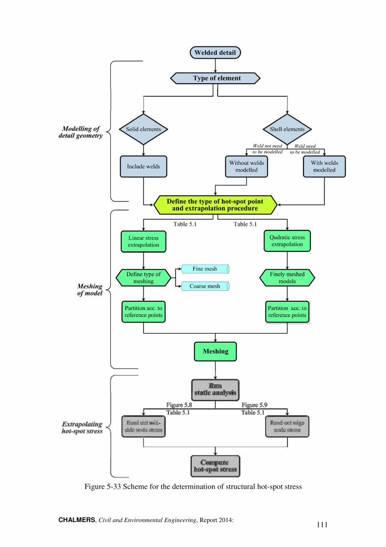
CHALMERS, Civil and Environmental Engineering, Report 2014: 111
Figure 5-33 Scheme for the determination of structural hot-spot stress
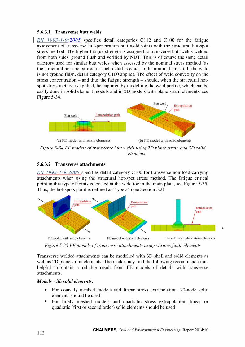
CHALMERS, Civil and Environmental Engineering, Report 2014:10 112
5.6.3.1 Transverse butt welds
EN 1993-1-9:2005 specifies detail categories C112 and C100 for the fatigue assessment of transverse full-penetration butt weld joints with the structural hot-spot stress method. The higher fatigue strength is assigned to transverse butt welds welded from both sides, ground flush and verified by NDT. This is of course the same detail category used for similar butt welds when assessed by the nominal stress method (as the structural hot-spot stress for such detail is equal to the nominal stress). If the weld is not ground flush, detail category C100 applies. The effect of weld convexity on the stress concentration – and thus the fatigue strength – should, when the structural hot-spot stress method is applied, be captured by modelling the weld profile, which can be easily done in solid element models and in 2D models with plane strain elements, see Figure 5-34.
Figure 5-34 FE models of transverse butt welds using 2D plane strain and 3D solid elements
5.6.3.2 Transverse attachments
EN 1993-1-9:2005 specifies detail category C100 for transverse non load-carrying attachments when using the structural hot-spot stress method. The fatigue critical point in this type of joints is located at the weld toe in the main plate, see Figure 5-35. Thus, the hot-spots point is defined as “type a” (see Section 5.2)
Figure 5-35 FE models of transverse attachments using various finite elements
Transverse welded attachments can be modelled with 3D shell and solid elements as well as 2D plane strain elements. The reader may find the following recommendations helpful to obtain a reliable result from FE models of details with transverse attachments.
Models with solid elements:
• For coarsely meshed models and linear stress extrapolation, 20-node solid elements should be used
• For finely meshed models and quadratic stress extrapolation, linear or quadratic (first or second order) solid elements should be used
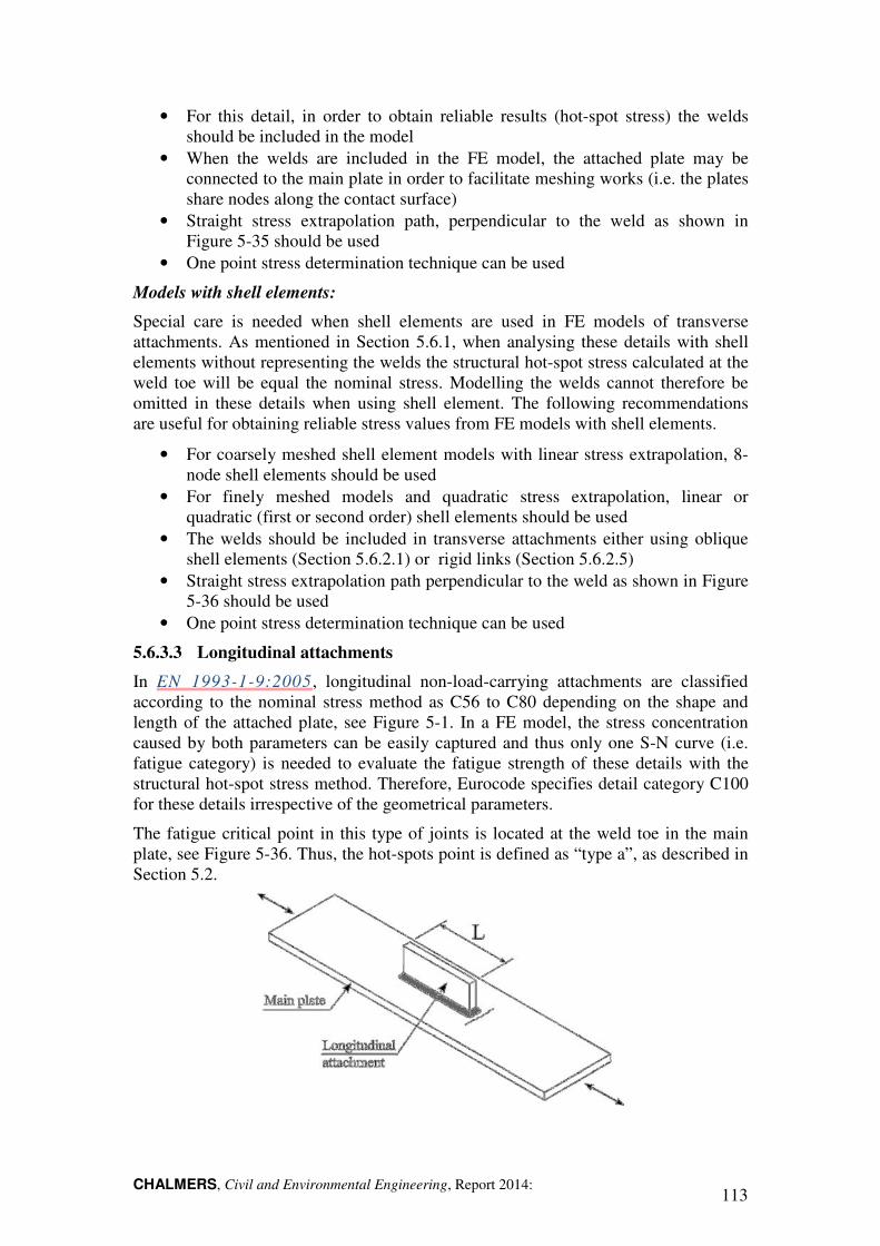
CHALMERS, Civil and Environmental Engineering, Report 2014: 113
• For this detail, in order to obtain reliable results (hot-spot stress) the welds should be included in the model
• When the welds are included in the FE model, the attached plate may be connected to the main plate in order to facilitate meshing works (i.e. the plates share nodes along the contact surface)
• Straight stress extrapolation path, perpendicular to the weld as shown in Figure 5-35 should be used
• One point stress determination technique can be used
Models with shell elements:
Special care is needed when shell elements are used in FE models of transverse attachments. As mentioned in Section 5.6.1, when analysing these details with shell elements without representing the welds the structural hot-spot stress calculated at the weld toe will be equal the nominal stress. Modelling the welds cannot therefore be omitted in these details when using shell element. The following recommendations are useful for obtaining reliable stress values from FE models with shell elements.
• For coarsely meshed shell element models with linear stress extrapolation, 8-node shell elements should be used
• For finely meshed models and quadratic stress extrapolation, linear or quadratic (first or second order) shell elements should be used
• The welds should be included in transverse attachments either using oblique shell elements (Section 5.6.2.1) or rigid links (Section 5.6.2.5)
• Straight stress extrapolation path perpendicular to the weld as shown in Figure 5-36 should be used
• One point stress determination technique can be used
5.6.3.3 Longitudinal attachments
In EN 1993-1-9:2005 , longitudinal non-load-carrying attachments are classified according to the nominal stress method as C56 to C80 depending on the shape and length of the attached plate, see Figure 5-1. In a FE model, the stress concentration caused by both parameters can be easily captured and thus only one S-N curve (i.e. fatigue category) is needed to evaluate the fatigue strength of these details with the structural hot-spot stress method. Therefore, Eurocode specifies detail category C100 for these details irrespective of the geometrical parameters.
The fatigue critical point in this type of joints is located at the weld toe in the main plate, see Figure 5-36. Thus, the hot-spots point is defined as “type a”, as described in Section 5.2.
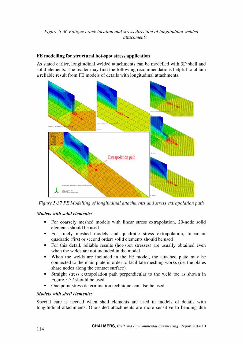
CHALMERS, Civil and Environmental Engineering, Report 2014:10 114
Figure 5-36 Fatigue crack location and stress direction of longitudinal welded attachments
FE modelling for structural hot-spot stress application
As stated earlier, longitudinal welded attachments can be modelled with 3D shell and solid elements. The reader may find the following recommendations helpful to obtain a reliable result from FE models of details with longitudinal attachments.
Figure 5-37 FE Modelling of longitudinal attachments and stress extrapolation path
Models with solid elements:
• For coarsely meshed models with linear stress extrapolation, 20-node solid elements should be used
• For finely meshed models and quadratic stress extrapolation, linear or quadratic (first or second order) solid elements should be used
• For this detail, reliable results (hot-spot stresses) are usually obtained even when the welds are not included in the model
• When the welds are included in the FE model, the attached plate may be connected to the main plate in order to facilitate meshing works (i.e. the plates share nodes along the contact surface)
• Straight stress extrapolation path perpendicular to the weld toe as shown in Figure 5-37 should be used
• One point stress determination technique can also be used
Models with shell elements:
Special care is needed when shell elements are used in models of details with longitudinal attachments. One-sided attachments are more sensitive to bending due
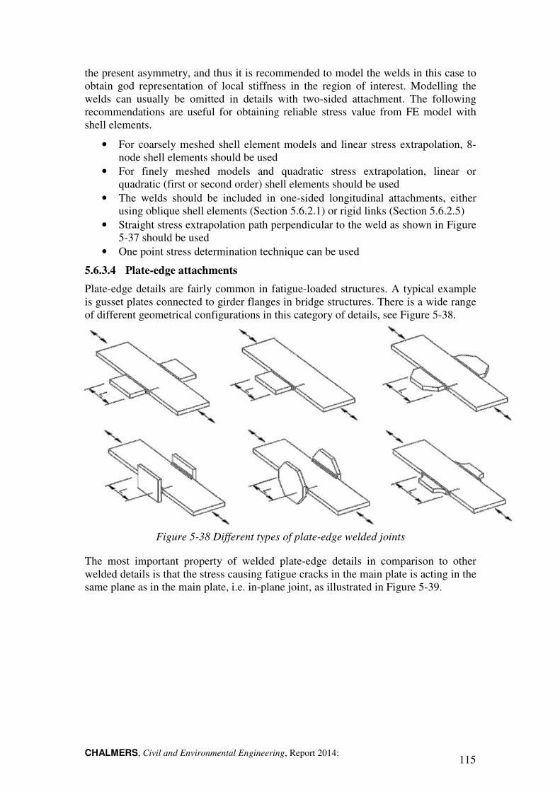
CHALMERS, Civil and Environmental Engineering, Report 2014: 115
the present asymmetry, and thus it is recommended to model the welds in this case to obtain god representation of local stiffness in the region of interest. Modelling the welds can usually be omitted in details with two-sided attachment. The following recommendations are useful for obtaining reliable stress value from FE model with shell elements.
• For coarsely meshed shell element models and linear stress extrapolation, 8-node shell elements should be used
• For finely meshed models and quadratic stress extrapolation, linear or quadratic (first or second order) shell elements should be used
• The welds should be included in one-sided longitudinal attachments, either using oblique shell elements (Section 5.6.2.1) or rigid links (Section 5.6.2.5)
• Straight stress extrapolation path perpendicular to the weld as shown in Figure 5-37 should be used
• One point stress determination technique can be used
5.6.3.4 Plate-edge attachments
Plate-edge details are fairly common in fatigue-loaded structures. A typical example is gusset plates connected to girder flanges in bridge structures. There is a wide range of different geometrical configurations in this category of details, see Figure 5-38.
Figure 5-38 Different types of plate-edge welded joints
The most important property of welded plate-edge details in comparison to other welded details is that the stress causing fatigue cracks in the main plate is acting in the same plane as in the main plate, i.e. in-plane joint, as illustrated in Figure 5-39.
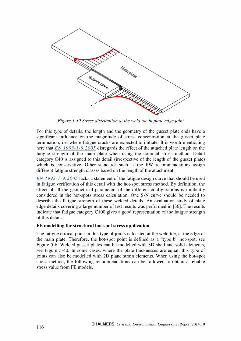
CHALMERS, Civil and Environmental Engineering, Report 2014:10 116
Figure 5-39 Stress distribution at the weld toe in plate edge joint
For this type of details, the length and the geometry of the gusset plate ends have a significant influence on the magnitude of stress concentration at the gusset plate termination; i.e. where fatigue cracks are expected to initiate. It is worth mentioning here that EN 1993-1-9.2005 disregards the effect of the attached plate length on the fatigue strength of the main plate when using the nominal stress method. Detail category C40 is assigned to this detail (irrespective of the length of the gusset plate) which is conservative. Other standards such as the IIW recommendations assign different fatigue strength classes based on the length of the attachment.
EN 1993-1-9:2005 lacks a statement of the fatigue design curve that should be used in fatigue verification of this detail with the hot-spot stress method. By definition, the effect of all the geometrical parameters of the different configurations is implicitly considered in the hot-spots stress calculation. One S-N curve should be needed to describe the fatigue strength of these welded details. An evaluation study of plate edge details covering a large number of test results was performed in [36]. The results indicate that fatigue category C100 gives a good representation of the fatigue strength of this detail.
FE modelling for structural hot-spot stress application
The fatigue critical point in this type of joints is located at the weld toe, at the edge of the main plate. Therefore, the hot-spot point is defined as a “type b” hot-spot, see Figure 5-6. Welded gusset plates can be modelled with 3D shell and solid elements, see Figure 5-40. In some cases, where the plate thicknesses are equal, this type of joints can also be modelled with 2D plane strain elements. When using the hot-spot stress method, the following recommendations can be followed to obtain a reliable stress value from FE models.
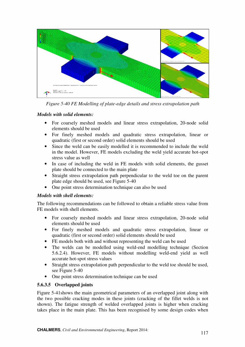
CHALMERS, Civil and Environmental Engineering, Report 2014: 117
Figure 5-40 FE Modelling of plate-edge details and stress extrapolation path
Models with solid elements:
• For coarsely meshed models and linear stress extrapolation, 20-node solid elements should be used
• For finely meshed models and quadratic stress extrapolation, linear or quadratic (first or second order) solid elements should be used
• Since the weld can be easily modelled it is recommended to include the weld in the model. However, FE models excluding the weld yield accurate hot-spot stress value as well
• In case of including the weld in FE models with solid elements, the gusset plate should be connected to the main plate
• Straight stress extrapolation path perpendicular to the weld toe on the parent plate edge should be used, see Figure 5-40
• One point stress determination technique can also be used
Models with shell elements:
The following recommendations can be followed to obtain a reliable stress value from FE models with shell elements.
• For coarsely meshed models and linear stress extrapolation, 20-node solid elements should be used
• For finely meshed models and quadratic stress extrapolation, linear or quadratic (first or second order) solid elements should be used
• FE models both with and without representing the weld can be used • The welds can be modelled using weld-end modelling technique (Section
5.6.2.4). However, FE models without modelling weld-end yield as well accurate hot-spot stress values
• Straight stress extrapolation path perpendicular to the weld toe should be used, see Figure 5-40
• One point stress determination technique can be used
5.6.3.5 Overlapped joints
Figure 5-41shows the main geometrical parameters of an overlapped joint along with the two possible cracking modes in these joints (cracking of the fillet welds is not shown). The fatigue strength of welded overlapped joints is higher when cracking takes place in the main plate. This has been recognised by some design codes when
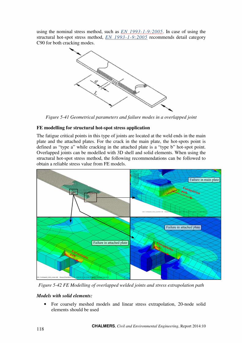
CHALMERS, Civil and Environmental Engineering, Report 2014:10 118
using the nominal stress method, such as EN 1993-1-9:2005. In case of using the structural hot-spot stress method, EN 1993-1-9:2005 recommends detail category C90 for both cracking modes.
Figure 5-41 Geometrical parameters and failure modes in a overlapped joint
FE modelling for structural hot-spot stress application
The fatigue critical points in this type of joints are located at the weld ends in the main plate and the attached plates. For the crack in the main plate, the hot-spots point is defined as “type a” while cracking in the attached plate is a “type b” hot-spot point. Overlapped joints can be modelled with 3D shell and solid elements. When using the structural hot-spot stress method, the following recommendations can be followed to obtain a reliable stress value from FE models.
Figure 5-42 FE Modelling of overlapped welded joints and stress extrapolation path
Models with solid elements:
• For coarsely meshed models and linear stress extrapolation, 20-node solid elements should be used
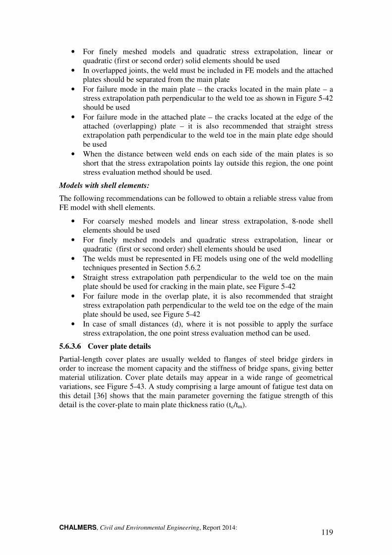
CHALMERS, Civil and Environmental Engineering, Report 2014: 119
• For finely meshed models and quadratic stress extrapolation, linear or quadratic (first or second order) solid elements should be used
• In overlapped joints, the weld must be included in FE models and the attached plates should be separated from the main plate
• For failure mode in the main plate – the cracks located in the main plate – a stress extrapolation path perpendicular to the weld toe as shown in Figure 5-42 should be used
• For failure mode in the attached plate – the cracks located at the edge of the attached (overlapping) plate – it is also recommended that straight stress extrapolation path perpendicular to the weld toe in the main plate edge should be used
• When the distance between weld ends on each side of the main plates is so short that the stress extrapolation points lay outside this region, the one point stress evaluation method should be used.
Models with shell elements:
The following recommendations can be followed to obtain a reliable stress value from FE model with shell elements.
• For coarsely meshed models and linear stress extrapolation, 8-node shell elements should be used
• For finely meshed models and quadratic stress extrapolation, linear or quadratic (first or second order) shell elements should be used
• The welds must be represented in FE models using one of the weld modelling techniques presented in Section 5.6.2
• Straight stress extrapolation path perpendicular to the weld toe on the main plate should be used for cracking in the main plate, see Figure 5-42
• For failure mode in the overlap plate, it is also recommended that straight stress extrapolation path perpendicular to the weld toe on the edge of the main plate should be used, see Figure 5-42
• In case of small distances (d), where it is not possible to apply the surface stress extrapolation, the one point stress evaluation method can be used.
5.6.3.6 Cover plate details
Partial-length cover plates are usually welded to flanges of steel bridge girders in order to increase the moment capacity and the stiffness of bridge spans, giving better material utilization. Cover plate details may appear in a wide range of geometrical variations, see Figure 5-43. A study comprising a large amount of fatigue test data on this detail [36] shows that the main parameter governing the fatigue strength of this detail is the cover-plate to main plate thickness ratio (tc/tm).
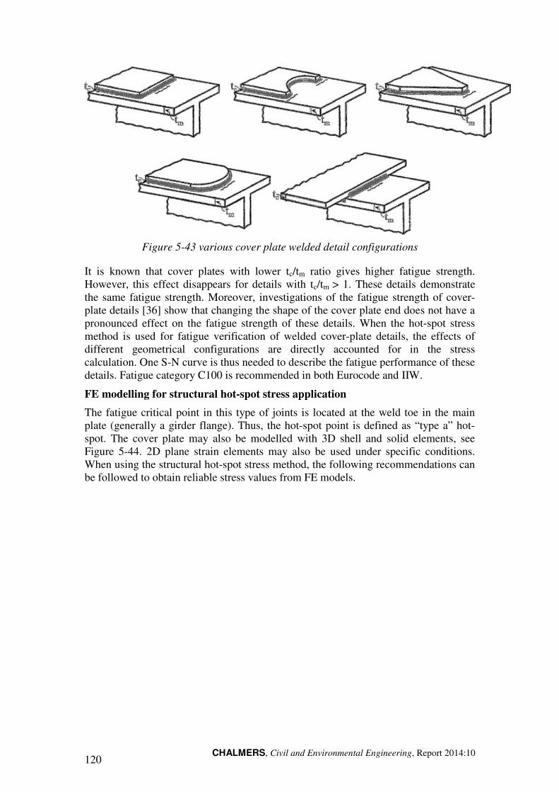
CHALMERS, Civil and Environmental Engineering, Report 2014:10 120
Figure 5-43 various cover plate welded detail configurations
It is known that cover plates with lower tc/tm ratio gives higher fatigue strength. However, this effect disappears for details with tc/tm > 1. These details demonstrate the same fatigue strength. Moreover, investigations of the fatigue strength of cover-plate details [36] show that changing the shape of the cover plate end does not have a pronounced effect on the fatigue strength of these details. When the hot-spot stress method is used for fatigue verification of welded cover-plate details, the effects of different geometrical configurations are directly accounted for in the stress calculation. One S-N curve is thus needed to describe the fatigue performance of these details. Fatigue category C100 is recommended in both Eurocode and IIW.
FE modelling for structural hot-spot stress application
The fatigue critical point in this type of joints is located at the weld toe in the main plate (generally a girder flange). Thus, the hot-spot point is defined as “type a” hot-spot. The cover plate may also be modelled with 3D shell and solid elements, see Figure 5-44. 2D plane strain elements may also be used under specific conditions. When using the structural hot-spot stress method, the following recommendations can be followed to obtain reliable stress values from FE models.
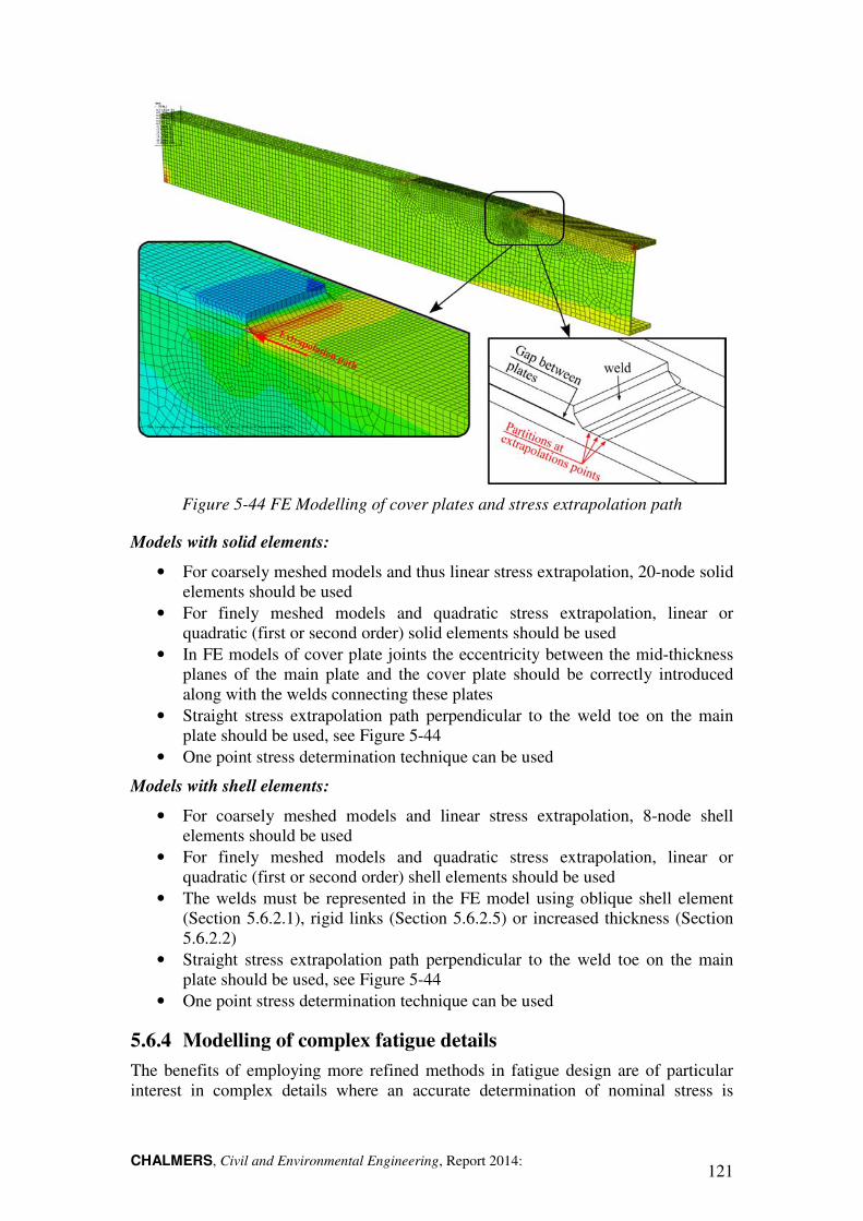
CHALMERS, Civil and Environmental Engineering, Report 2014: 121
Figure 5-44 FE Modelling of cover plates and stress extrapolation path
Models with solid elements:
• For coarsely meshed models and thus linear stress extrapolation, 20-node solid elements should be used
• For finely meshed models and quadratic stress extrapolation, linear or quadratic (first or second order) solid elements should be used
• In FE models of cover plate joints the eccentricity between the mid-thickness planes of the main plate and the cover plate should be correctly introduced along with the welds connecting these plates
• Straight stress extrapolation path perpendicular to the weld toe on the main plate should be used, see Figure 5-44
• One point stress determination technique can be used
Models with shell elements:
• For coarsely meshed models and linear stress extrapolation, 8-node shell elements should be used
• For finely meshed models and quadratic stress extrapolation, linear or quadratic (first or second order) shell elements should be used
• The welds must be represented in the FE model using oblique shell element (Section 5.6.2.1), rigid links (Section 5.6.2.5) or increased thickness (Section 5.6.2.2)
• Straight stress extrapolation path perpendicular to the weld toe on the main plate should be used, see Figure 5-44
• One point stress determination technique can be used
5.6.4 Modelling of complex fatigue details
The benefits of employing more refined methods in fatigue design are of particular interest in complex details where an accurate determination of nominal stress is
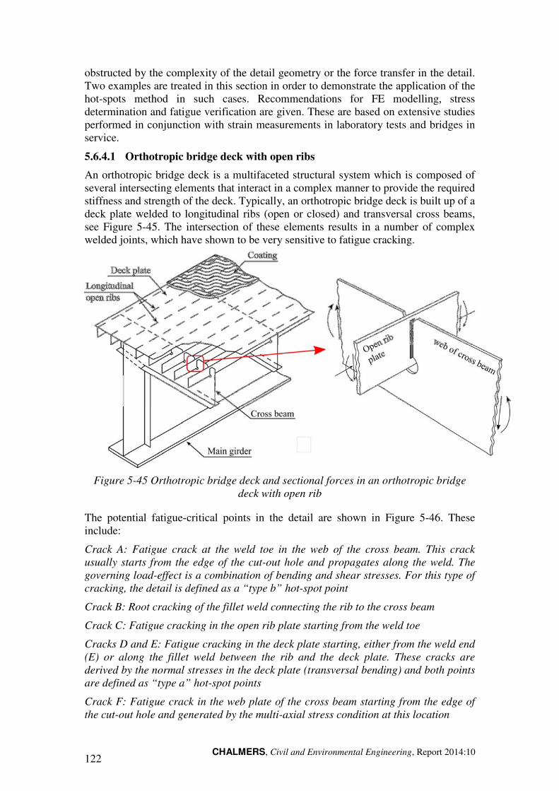
CHALMERS, Civil and Environmental Engineering, Report 2014:10 122
obstructed by the complexity of the detail geometry or the force transfer in the detail. Two examples are treated in this section in order to demonstrate the application of the hot-spots method in such cases. Recommendations for FE modelling, stress determination and fatigue verification are given. These are based on extensive studies performed in conjunction with strain measurements in laboratory tests and bridges in service.
5.6.4.1 Orthotropic bridge deck with open ribs
An orthotropic bridge deck is a multifaceted structural system which is composed of several intersecting elements that interact in a complex manner to provide the required stiffness and strength of the deck. Typically, an orthotropic bridge deck is built up of a deck plate welded to longitudinal ribs (open or closed) and transversal cross beams, see Figure 5-45. The intersection of these elements results in a number of complex welded joints, which have shown to be very sensitive to fatigue cracking.
Figure 5-45 Orthotropic bridge deck and sectional forces in an orthotropic bridge deck with open rib
The potential fatigue-critical points in the detail are shown in Figure 5-46. These include:
Crack A: Fatigue crack at the weld toe in the web of the cross beam. This crack usually starts from the edge of the cut-out hole and propagates along the weld. The governing load-effect is a combination of bending and shear stresses. For this type of cracking, the detail is defined as a “type b” hot-spot point
Crack B: Root cracking of the fillet weld connecting the rib to the cross beam
Crack C: Fatigue cracking in the open rib plate starting from the weld toe
Cracks D and E: Fatigue cracking in the deck plate starting, either from the weld end (E) or along the fillet weld between the rib and the deck plate. These cracks are derived by the normal stresses in the deck plate (transversal bending) and both points are defined as “type a” hot-spot points
Crack F: Fatigue crack in the web plate of the cross beam starting from the edge of the cut-out hole and generated by the multi-axial stress condition at this location
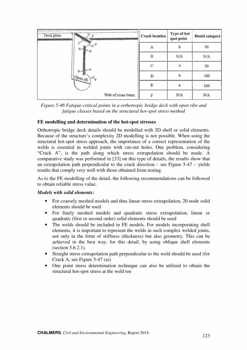
CHALMERS, Civil and Environmental Engineering, Report 2014: 123
Figure 5-46 Fatigue critical points in a orthotropic bridge deck with open ribs and fatigue classes based on the structural hot-spot stress method
FE modelling and determination of the hot-spot stresses
Orthotropic bridge deck details should be modelled with 3D shell or solid elements. Because of the structure’s complexity 2D modelling is not possible. When using the structural hot-spot stress approach, the importance of a correct representation of the welds is essential in welded joints with cut-out holes. One problem, considering “Crack A”, is the path along which stress extrapolation should be made. A comparative study was performed in [33] on this type of details, the results show that an extrapolation path perpendicular to the crack direction – see Figure 5-47 – yields results that comply very well with those obtained from testing.
As to the FE modelling of the detail, the following recommendations can be followed to obtain reliable stress value.
Models with solid elements:
• For coarsely meshed models and thus linear stress extrapolation, 20-node solid elements should be used
• For finely meshed models and quadratic stress extrapolation, linear or quadratic (first or second order) solid elements should be used
• The welds should be included in FE models. For models incorporating shell elements, it is important to represent the welds in such complex welded joints, not only in the form of stiffness (thickness) but also geometry. This can be achieved in the best way, for this detail, by using oblique shell elements (section 5.6.2.1).
• Straight stress extrapolation path perpendicular to the weld should be used (for Crack A, see Figure 5-47 (a))
• One point stress determination technique can also be utilized to obtain the structural hot-spot stress at the weld toe
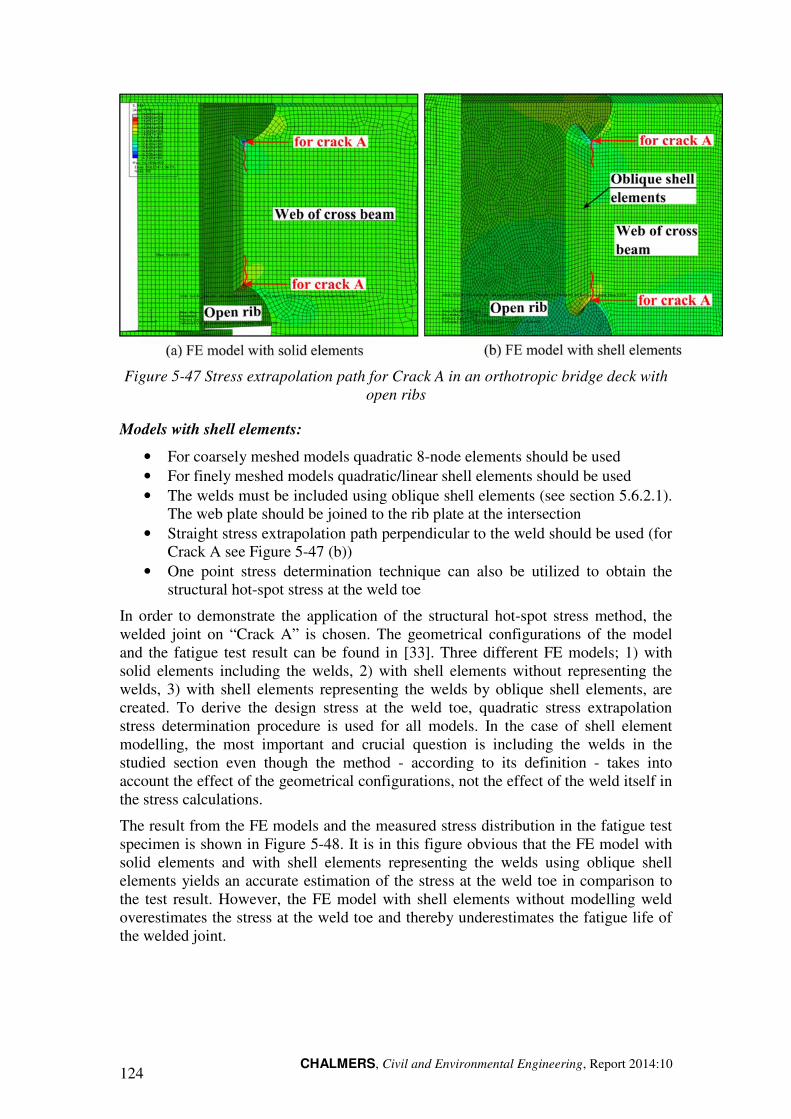
CHALMERS, Civil and Environmental Engineering, Report 2014:10 124
Figure 5-47 Stress extrapolation path for Crack A in an orthotropic bridge deck with open ribs
Models with shell elements:
• For coarsely meshed models quadratic 8-node elements should be used • For finely meshed models quadratic/linear shell elements should be used • The welds must be included using oblique shell elements (see section 5.6.2.1).
The web plate should be joined to the rib plate at the intersection • Straight stress extrapolation path perpendicular to the weld should be used (for
Crack A see Figure 5-47 (b)) • One point stress determination technique can also be utilized to obtain the
structural hot-spot stress at the weld toe
In order to demonstrate the application of the structural hot-spot stress method, the welded joint on “Crack A” is chosen. The geometrical configurations of the model and the fatigue test result can be found in [33]. Three different FE models; 1) with solid elements including the welds, 2) with shell elements without representing the welds, 3) with shell elements representing the welds by oblique shell elements, are created. To derive the design stress at the weld toe, quadratic stress extrapolation stress determination procedure is used for all models. In the case of shell element modelling, the most important and crucial question is including the welds in the studied section even though the method - according to its definition - takes into account the effect of the geometrical configurations, not the effect of the weld itself in the stress calculations.
The result from the FE models and the measured stress distribution in the fatigue test specimen is shown in Figure 5-48. It is in this figure obvious that the FE model with solid elements and with shell elements representing the welds using oblique shell elements yields an accurate estimation of the stress at the weld toe in comparison to the test result. However, the FE model with shell elements without modelling weld overestimates the stress at the weld toe and thereby underestimates the fatigue life of the welded joint.
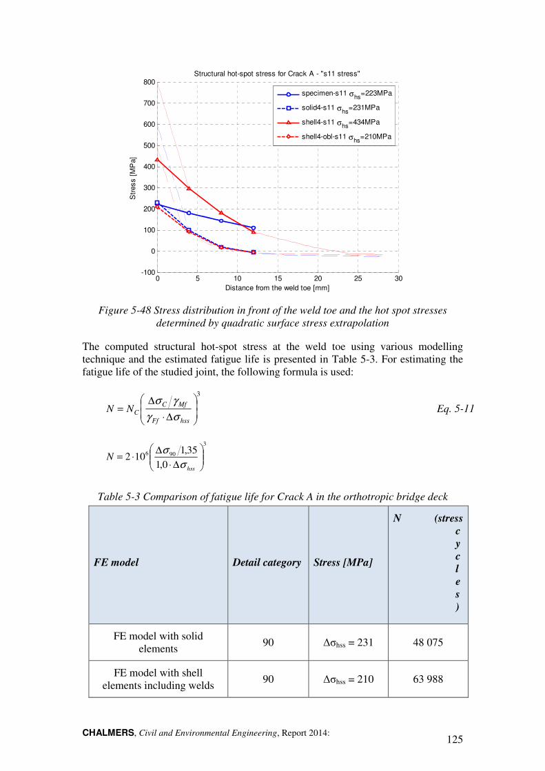
CHALMERS, Civil and Environmental Engineering, Report 2014: 125
Figure 5-48 Stress distribution in front of the weld toe and the hot spot stresses determined by quadratic surface stress extrapolation
The computed structural hot-spot stress at the weld toe using various modelling technique and the estimated fatigue life is presented in Table 5-3. For estimating the fatigue life of the studied joint, the following formula is used:
3
∆⋅
∆=
hssFf
MfCCNN
σγ
γσ Eq. 5-11
3
906
0,135,1
102
∆⋅
∆⋅=
hss
Nσ
σ
Table 5-3 Comparison of fatigue life for Crack A in the orthotropic bridge deck
FE model Detail category Stress [MPa]
N (stress cycles)
FE model with solid elements
90 ∆σhss = 231 48 075
FE model with shell elements including welds
90 ∆σhss = 210 63 988
0 5 10 15 20 25 30-100
0
100
200
300
400
500
600
700
800Structural hot-spot stress for Crack A - "s11 stress"
Distance from the weld toe [mm]
Str
ess [
MP
a]
specimen-s11 σhs=223MPa
solid4-s11 σhs=231MPa
shell4-s11 σhs=434MPa
shell4-obl-s11 σhs=210MPa
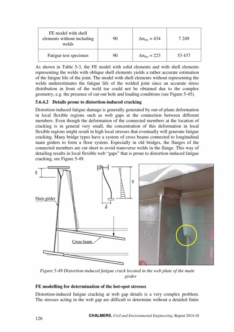
CHALMERS, Civil and Environmental Engineering, Report 2014:10 126
FE model with shell elements without including
welds 90 ∆σhss = 434 7 249
Fatigue test specimen 90 ∆σhss = 223 53 437
As shown in Table 5-3, the FE model with solid elements and with shell elements representing the welds with oblique shell elements yields a rather accurate estimation of the fatigue life of the joint. The model with shell elements without representing the welds underestimates the fatigue life of the welded joint since an accurate stress distribution in front of the weld toe could not be obtained due to the complex geometry, e.g. the presence of cut-out hole and loading conditions (see Figure 5-45).
5.6.4.2 Details prone to distortion-induced cracking
Distortion-induced fatigue damage is generally generated by out-of-plane deformation in local flexible regions such as web gaps at the connection between different members. Even though the deformation of the connected members at the location of cracking is in general very small, the concentration of this deformation in local flexible regions might result in high local stresses that eventually will generate fatigue cracking. Many bridge types have a system of cross beams connected to longitudinal main girders to form a floor system. Especially in old bridges, the flanges of the connected members are cut short to avoid transverse welds in the flange. This way of detailing results in local flexible web “gaps” that is prone to distortion-induced fatigue cracking, see Figure 5-49.
Figure 5-49 Distortion-induced fatigue crack located in the web plate of the main girder
FE modelling for determination of the hot-spot stresses
Distortion-induced fatigue cracking at web gap details is a very complex problem. The stresses acting in the web gap are difficult to determine without a detailed finite
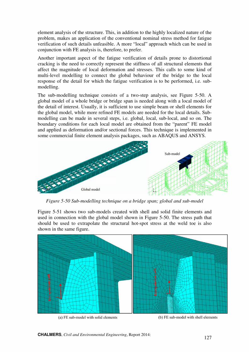
CHALMERS, Civil and Environmental Engineering, Report 2014: 127
element analysis of the structure. This, in addition to the highly localized nature of the problem, makes an application of the conventional nominal stress method for fatigue verification of such details unfeasible. A more “local” approach which can be used in conjunction with FE analysis is, therefore, to prefer.
Another important aspect of the fatigue verification of details prone to distortional cracking is the need to correctly represent the stiffness of all structural elements that affect the magnitude of local deformation and stresses. This calls to some kind of multi-level modelling to connect the global behaviour of the bridge to the local response of the detail for which the fatigue verification is to be performed, i.e. sub-modelling.
The sub-modelling technique consists of a two-step analysis, see Figure 5-50. A global model of a whole bridge or bridge span is needed along with a local model of the detail of interest. Usually, it is sufficient to use simple beam or shell elements for the global model, while more refined FE models are needed for the local details. Sub-modelling can be made in several steps, i.e. global, local, sub-local, and so on. The boundary conditions for each local model are obtained from the “parent” FE model and applied as deformation and/or sectional forces. This technique is implemented in some commercial finite element analysis packages, such as ABAQUS and ANSYS.
Figure 5-50 Sub-modelling technique on a bridge span; global and sub-model
Figure 5-51 shows two sub-models created with shell and solid finite elements and used in connection with the global model shown in Figure 5-50. The stress path that should be used to extrapolate the structural hot-spot stress at the weld toe is also shown in the same figure.
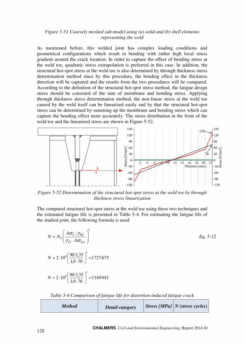
CHALMERS, Civil and Environmental Engineering, Report 2014:10 128
Figure 5-51 Coarsely meshed sub-model using (a) solid and (b) shell elements representing the weld
As mentioned before, this welded joint has complex loading conditions and geometrical configurations which result in bending with rather high local stress gradient around the crack location. In order to capture the effect of bending stress at the weld toe, quadratic stress extrapolation is preferred in this case. In addition, the structural hot-spot stress at the weld toe is also determined by through thickness stress determination method since by this procedure, the bending effect in the thickness direction will be captured and the results from the two procedures will be compared. According to the definition of the structural hot-spot stress method, the fatigue design stress should be consisted of the sum of membrane and bending stress. Applying through thickness stress determination method, the non-linear stress at the weld toe caused by the weld itself can be linearized easily and by that the structural hot-spot stress can be determined by summing up the membrane and bending stress which can capture the bending effect more accurately. The stress distribution in the front of the weld toe and the linearized stress are shown in Figure 5-52.
Figure 5-52 Determination of the structural hot-spot stress at the weld toe by through thickness stress linearization
The computed structural hot-spot stress at the weld toe using these two techniques and the estimated fatigue life is presented in Table 5-4. For estimating the fatigue life of the studied joint, the following formula is used:
3
∆⋅
∆=
hssFf
MfCCNN
σγ
γσ Eq. 5-12
6757271700,135,190
1023
6 =
⋅⋅=N
9433491760,135,190
1023
6 =
⋅⋅=N
Table 5-4 Comparison of fatigue life for distortion-induced fatigue crack
Method Detail category Stress [MPa] N (stress cycles)
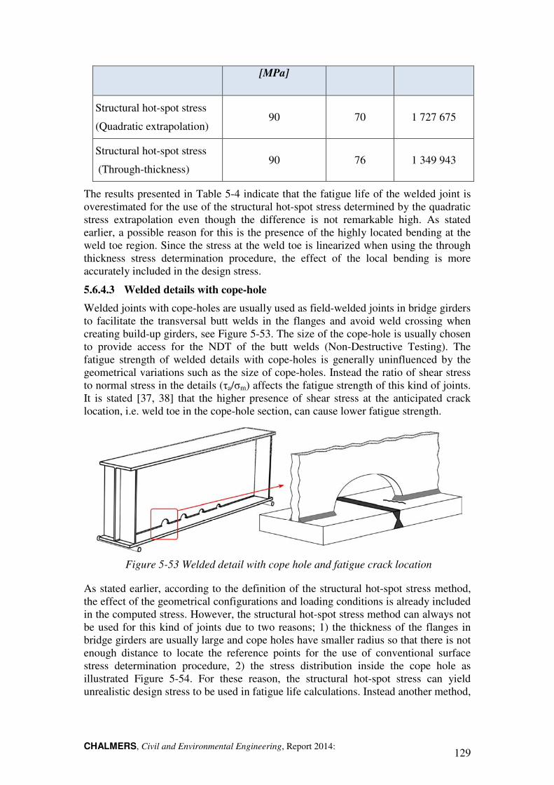
CHALMERS, Civil and Environmental Engineering, Report 2014: 129
[MPa]
Structural hot-spot stress
(Quadratic extrapolation) 90 70 1 727 675
Structural hot-spot stress
(Through-thickness) 90 76 1 349 943
The results presented in Table 5-4 indicate that the fatigue life of the welded joint is overestimated for the use of the structural hot-spot stress determined by the quadratic stress extrapolation even though the difference is not remarkable high. As stated earlier, a possible reason for this is the presence of the highly located bending at the weld toe region. Since the stress at the weld toe is linearized when using the through thickness stress determination procedure, the effect of the local bending is more accurately included in the design stress.
5.6.4.3 Welded details with cope-hole
Welded joints with cope-holes are usually used as field-welded joints in bridge girders to facilitate the transversal butt welds in the flanges and avoid weld crossing when creating build-up girders, see Figure 5-53. The size of the cope-hole is usually chosen to provide access for the NDT of the butt welds (Non-Destructive Testing). The fatigue strength of welded details with cope-holes is generally uninfluenced by the geometrical variations such as the size of cope-holes. Instead the ratio of shear stress to normal stress in the details (τa/σm) affects the fatigue strength of this kind of joints. It is stated [37, 38] that the higher presence of shear stress at the anticipated crack location, i.e. weld toe in the cope-hole section, can cause lower fatigue strength.
Figure 5-53 Welded detail with cope hole and fatigue crack location
As stated earlier, according to the definition of the structural hot-spot stress method, the effect of the geometrical configurations and loading conditions is already included in the computed stress. However, the structural hot-spot stress method can always not be used for this kind of joints due to two reasons; 1) the thickness of the flanges in bridge girders are usually large and cope holes have smaller radius so that there is not enough distance to locate the reference points for the use of conventional surface stress determination procedure, 2) the stress distribution inside the cope hole as illustrated Figure 5-54. For these reason, the structural hot-spot stress can yield unrealistic design stress to be used in fatigue life calculations. Instead another method,
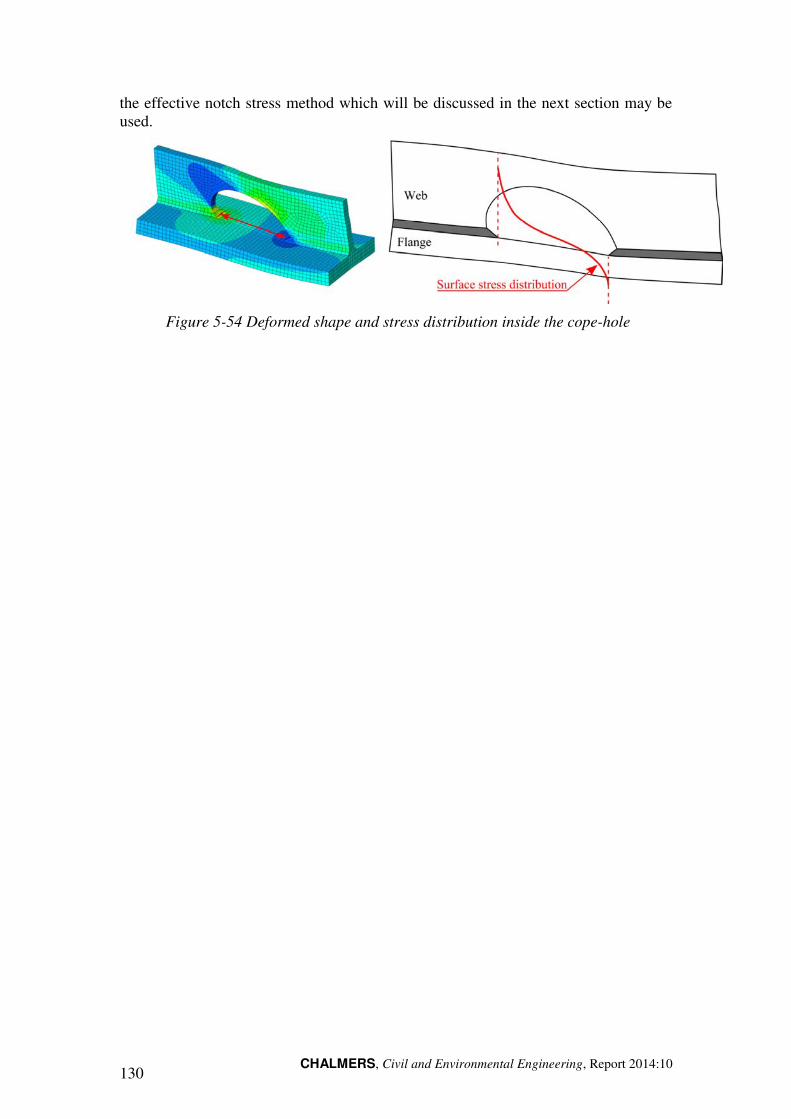
CHALMERS, Civil and Environmental Engineering, Report 2014:10 130
the effective notch stress method which will be discussed in the next section may be used.
Figure 5-54 Deformed shape and stress distribution inside the cope-hole
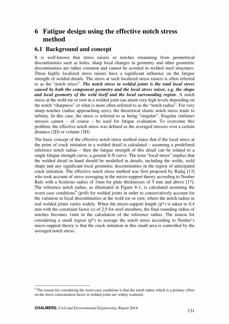
CHALMERS, Civil and Environmental Engineering, Report 2014: 131
6 Fatigue design using the effective notch stress
method
6.1 Background and concept
It is well-known that stress raisers or notches emanating from geometrical discontinuities such as holes, sharp local changes in geometry and other geometric discontinuities are rather common and cannot be avoided in welded steel structures. These highly localized stress raisers have a significant influence on the fatigue strength of welded details. The stress at such localized stress raisers is often referred to as the “notch stress”. The notch stress in welded joints is the total local stress caused by both the component geometry and the local stress raiser, e.g. the shape and local geometry of the weld itself and the local surrounding region. A notch stress at the weld toe or root in a welded joint can attain very high levels depending on the notch “sharpness” or what is more often referred to as the “notch radius”. For very sharp notches (radius approaching zero), the theoretical elastic notch stress tends to infinity. In this case, the stress is referred to as being “singular”. Singular (infinite) stresses cannot – of course – be used for fatigue evaluation. To overcome this problem, the effective notch stress was defined as the averaged stresses over a certain distance (2D) or volume (3D).
The basic concept of the effective notch stress method states that if the local stress at the point of crack initiation in a welded detail is calculated – assuming a predefined reference notch radius – then the fatigue strength of this detail can be related to a single fatigue strength curve, a general S-N curve. The term “local stress” implies that the welded detail in hand should be modelled in details, including the welds, weld shape and any significant local geometric discontinuities in the region of anticipated crack initiation. The effective notch stress method was first proposed by Radaj [13] who took account of stress averaging in the micro-support theory according to Neuber Rule with a fictitious radius of 1mm for plate thicknesses of 5 mm and above [17]. The reference notch radius, as illustrated in Figure 6-1, is calculated assuming the worst case conditions8 (ρ=0) for welded joints in order to conservatively account for the variation in local discontinuities at the weld toe or root, where the notch radius in real welded joints varies widely. When the micro-support length (ρ*) is taken to 0,4 mm with the constraint factor (s) of 2,5 for steel members, the final rounding radius of notches becomes 1mm in the calculation of the reference radius. The reason for considering a small region (ρ*) to average the notch stress according to Neuber’s micro-support theory is that the crack initiation in this small area is controlled by the averaged notch stress.
8 The reason for considering the worst case conditions is that the notch radius which is a primary effect on the stress concentration factor in welded joints are widely scattered.
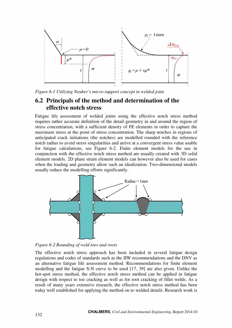
CHALMERS, Civil and Environmental Engineering, Report 2014:10 132
Figure 6-1 Utilizing Neuber’s micro-support concept in welded joint
6.2 Principals of the method and determination of the
effective notch stress
Fatigue life assessment of welded joints using the effective notch stress method requires rather accurate definition of the detail geometry in and around the region of stress concentration, with a sufficient density of FE elements in order to capture the maximum stress at the point of stress concentration. The sharp notches in regions of anticipated crack initiations (the notches) are modelled rounded with the reference notch radius to avoid stress singularities and arrive at a convergent stress value usable for fatigue calculations, see Figure 6-2. Finite element models for the use in conjunction with the effective notch stress method are usually created with 3D solid element models. 2D plane strain element models can however also be used for cases when the loading and geometry allow such an idealization. Two-dimensional models usually reduce the modelling efforts significantly.
Figure 6-2 Rounding of weld toes and roots
The effective notch stress approach has been included in several fatigue design regulations and codes of standards such as the IIW recommendations and the DNV as an alternative fatigue life assessment method. Recommendations for finite element modelling and the fatigue S-N curve to be used [17, 39] are also given. Unlike the hot-spot stress method, the effective notch stress method can be applied in fatigue design with respect to toe cracking as well as for root cracking of fillet welds. As a result of many years extensive research, the effective notch stress method has been today well established for applying the method on to welded details. Research work is
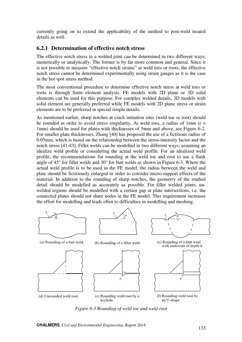
CHALMERS, Civil and Environmental Engineering, Report 2014: 133
currently going on to extend the applicability of the method to post-weld treated details as well.
6.2.1 Determination of effective notch stress
The effective notch stress in a welded joint can be determined in two different ways; numerically or analytically. The former is by far more common and general. Since it is not possible to measure “effective notch strains” at weld toes or roots, the effective notch stress cannot be determined experimentally using strain gauges as it is the case in the hot spot stress method.
The most conventional procedure to determine effective notch stress at weld toes or roots is through finite element analysis. FE models with 2D plane or 3D solid elements can be used for this purpose. For complex welded details, 3D models with solid element are generally preferred while FE models with 2D plane stress or strain elements are to be preferred in special simple details.
As mentioned earlier, sharp notches at crack initiation sites (weld toe or root) should be rounded in order to avoid stress singularity. At weld toes, a radius of 1mm (r = 1mm) should be used for plates with thicknesses of 5mm and above, see Figure 6-2. For smaller plate thicknesses, Zhang [40] has proposed the use of a fictitious radius of 0.05mm, which is based on the relationship between the stress-intensity factor and the notch stress [41-43]. Fillet welds can be modelled in two different ways; assuming an idealize weld profile or considering the actual weld profile. For an idealized weld profile, the recommendations for rounding at the weld toe and root to use a flank angle of 45° for fillet welds and 30° for butt welds as shown in Figure 6-3. Where the actual weld profile is to be used in the FE model, the radius between the weld and plate should be fictitiously enlarged in order to consider micro-support effects of the material. In addition to the rounding of sharp notches, the geometry of the studied detail should be modelled as accurately as possible. For fillet welded joints, un-welded regions should be modelled with a certain gap at plate intersections, i.e. the connected plates should not share nodes in the FE model. This requirement increases the effort for modelling and leads often to difficulties in modelling and meshing.
Figure 6-3 Rounding of weld toe and weld root

CHALMERS, Civil and Environmental Engineering, Report 2014:10 134
As shown in Figure 6-3, modelling of the weld root can be performed in two different ways; the so called keyhole and U-shape. The choice of root shape is more or less controlled by the type of weld. In load-carrying welds, both root shapes yield usually the same effective notch stress while in non-load-carrying welds, the effective stress range is lower with the U-shape weld root than with the keyhole weld root. This means that the fatigue strength can be underestimated with U-shape root configuration whereas the fatigue strength can be overestimated with keyhole configuration in non-load-carrying welds. The IIW recommendations suggests therefore using U-shape root configuration when determining the effective notch stress with reference to root cracking in details with load-carrying welds [44].
As to the type and size of FE-elements in the notch region, the recommendations given by the IIW are reproduced in Table 6-1 and illustrated in Figure 6-4.
Table 6-1 IIW Recommendations for FE models when using the effective notch stress [44]
Element type
Element size
Relative size r = 1mm
(t ≥ 5mm)
r = 0.05mm
(t < 5mm)
Hexahedral Quadratic ≤ r / 4 0.25mm 0.012mm
Linear ≤ r / 6 0.15mm 0.008mm
Tetrahedral Quadratic ≤ r / 6 0.15mm 0.008mm
Figure 6-4 Recommended mesh density using tetrahedral and hexahedral elements for an effective notch analysis
6.2.2 Fatigue life evaluation using the effective notch stress
As the effective notch stress covers the global stress concentration effects as well as the effect of local geometry, a single S-N curve should be sufficient to represent the fatigue strength of any welded detail. Eurocode lacks any recommendations with reference to the effective notch stress method.
The recommendations in this Chapter are based on the state-of-the-art research on the application of the effective notch stress in fatigue verification of welded joints.
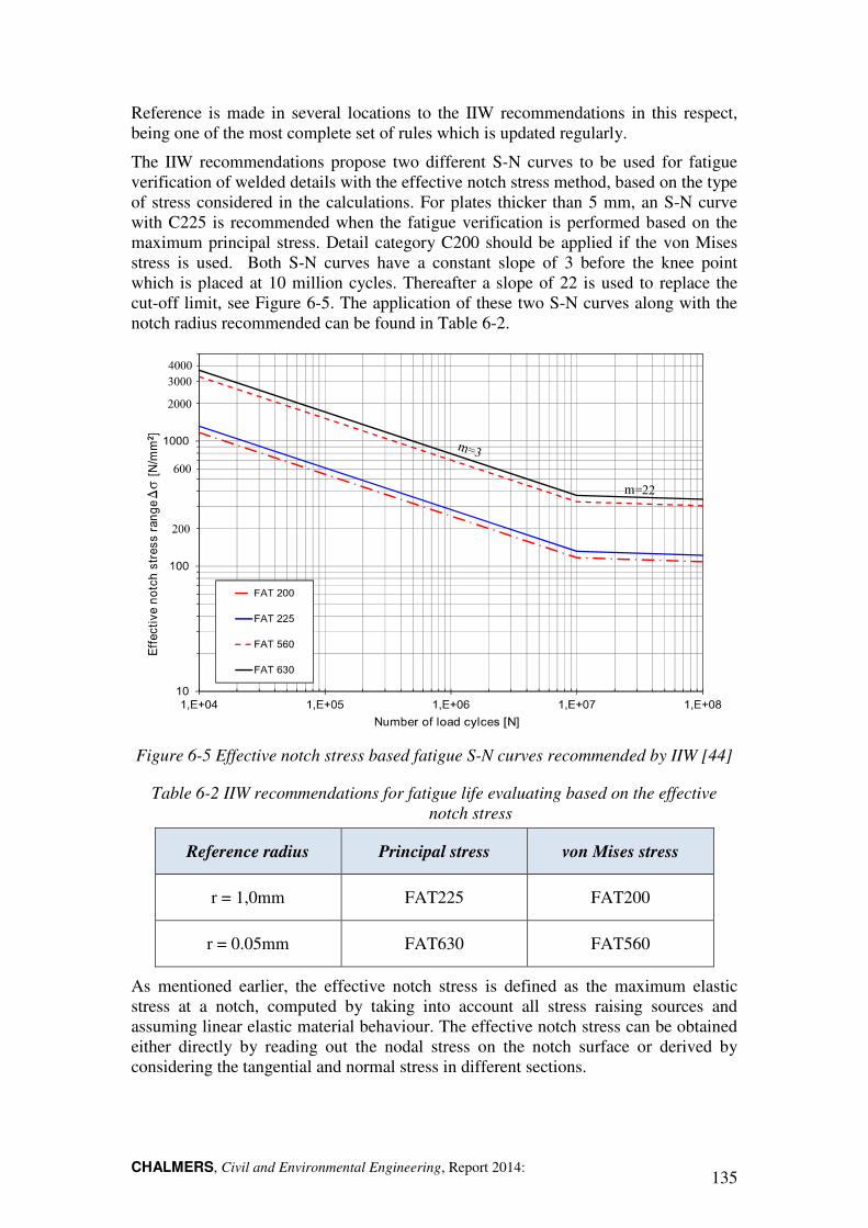
CHALMERS, Civil and Environmental Engineering, Report 2014: 135
Reference is made in several locations to the IIW recommendations in this respect, being one of the most complete set of rules which is updated regularly.
The IIW recommendations propose two different S-N curves to be used for fatigue verification of welded details with the effective notch stress method, based on the type of stress considered in the calculations. For plates thicker than 5 mm, an S-N curve with C225 is recommended when the fatigue verification is performed based on the maximum principal stress. Detail category C200 should be applied if the von Mises stress is used. Both S-N curves have a constant slope of 3 before the knee point which is placed at 10 million cycles. Thereafter a slope of 22 is used to replace the cut-off limit, see Figure 6-5. The application of these two S-N curves along with the notch radius recommended can be found in Table 6-2.
Figure 6-5 Effective notch stress based fatigue S-N curves recommended by IIW [44]
Table 6-2 IIW recommendations for fatigue life evaluating based on the effective notch stress
Reference radius Principal stress von Mises stress
r = 1,0mm FAT225 FAT200
r = 0.05mm FAT630 FAT560
As mentioned earlier, the effective notch stress is defined as the maximum elastic stress at a notch, computed by taking into account all stress raising sources and assuming linear elastic material behaviour. The effective notch stress can be obtained either directly by reading out the nodal stress on the notch surface or derived by considering the tangential and normal stress in different sections.
CHALMERS, Civil and Environmental Engineering, Report 2014:10 136
In a detail that experiences a uniaxial state of stress at the location of crack initiation, the maximum principal stress gives a good representation of the fatigue deriving stress range at this location. If stress multiaxiality exists, however, the direction of the principal stress might be constant (proportional loading) or will vary - to both magnitude and direction - over the loading cycle. In both cases, another (scalar) stress is needed to relate the load effects to the fatigue life in a more representative way.
Fatigue verification with the effective notch stress method under stress multiaxiality is still a subject for on-going research. Therefore, complex loading situations with non-proportional loading are left outside this handbook. For details experiencing proportional multiaxial stress at the location of crack initiation, the following recommendations apply:
1. If the first and second principal stresses have the same sign, the first (maximum) principal stress should be used in the fatigue verification,
2. Otherwise, the equivalent von Mises stress using the range of stress components should be used.
It should also be mentioned here that the effective notch stress method is not applicable if there is a significant stress component parallel to the weld. In such cases, fatigue evaluation is more appropriately performed with the nominal stress method.
6.2.2.1 Thickness and misalignment correlation factor
Unlike the nominal and the hot-spot stress methods, the thickness effects do not need to be considered (by a reduction of the fatigue strength) when the fatigue verification is performed with the effective notch stress method. These effects are already “accounted for” on the load effect side (i.e. in the calculated notch stress) as the stress in the thickness direction increases with increased thickness on account of r/t ratio [44]. There is therefore no need for any thickness correction factor in this method. In the presence of significant misalignments, the effect of these can also be easily considered in the stress calculations by modelling the actual misalignment. Of course, it is also possible to apply a correction factor to take into account misalignment effect without including it into FE models.
6.3 Recommendations for finite element modelling
As stated earlier, the effective notch stress method is applicable for 2D plane and 3D solid finite element models and requires an accurately defined FE model. This means that FE models to be used for determining the effective notch stress should reproduce the “exact” geometry of the studied detail, including welds. Gaps between plates in fillet welded joints and any major misalignments not covered by the S-N curve should also be accounted for. FE models with shell elements should not be used in fatigue verification with the effective notch stress method. For simple loading conditions in which the stresses in the transverse direction is negligible, 2D plane-stress elements can be used. Welded steel structures contain rarely simple details or simple loading conditions so 3D solid element models are usually preferred. Building finite element models with solid elements in large structures can, however, easily lead to large FE models that require very long computation time and heavy data to handle. To overcome this problem, sub-modelling can be used to analyse smaller parts of the structure.
CHALMERS, Civil and Environmental Engineering, Report 2014: 137
6.3.1 Sub-modelling
The purpose of using sub-modelling technique is commonly to obtain a more detailed result (stresses and deformation) in local regions which are of special interest for design. Therefore, sub-models are constructed with more details and equipped with much finer mesh than the global model to which they belong.
A Sub-modelling technique includes, thus, a two-step analysis: an analysis of the global structure; and a refined analysis of a detail in that structure. The global model and the sub-model are usually two distinct finite element models. The global model is usually a simplified representation of the whole structure with minimum detailing and with a fairly coarse mesh. The sub-model, on the other hand, is usually constructed of a smaller part of the structure with a sufficiently detailed representation of local details that are judged to affect the load effects in the region of interest. Being as such, sub-models usually require fine meshing and more modelling efforts. It is important to notice that in a sub-model, the coordinates at the cut-regions should be same as those in the global model. The boundary conditions along the ”cutting edges” in a sub-model are obtained from the global model, either as displacements or sectional forces/stresses.
The procedure for determining the effective notch stress using the sub-modelling technique is given in Figure 6-6.
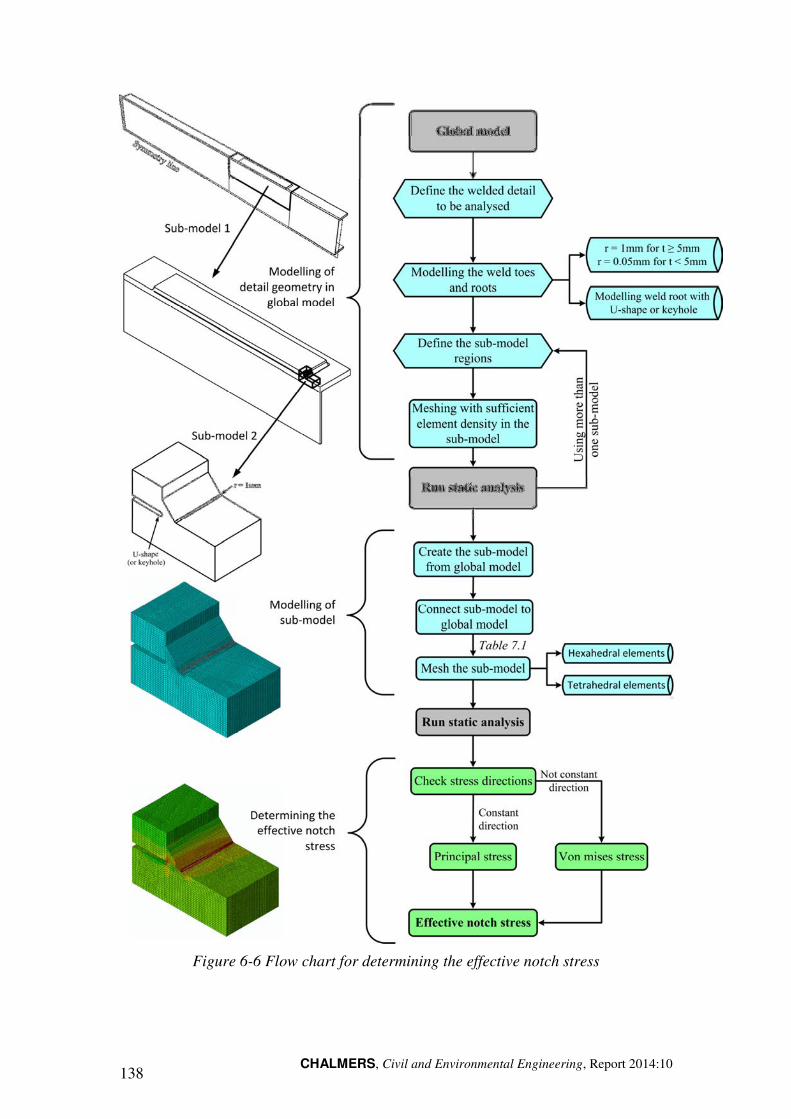
CHALMERS, Civil and Environmental Engineering, Report 2014:10 138
Figure 6-6 Flow chart for determining the effective notch stress
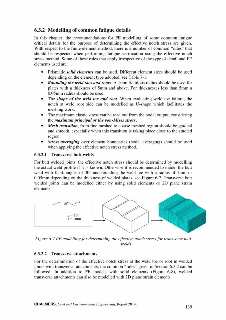
CHALMERS, Civil and Environmental Engineering, Report 2014: 139
6.3.2 Modelling of common fatigue details
In this chapter, the recommendations for FE modelling of some common fatigue critical details for the purpose of determining the effective notch stress are given. With respect to the finite element method, there is a number of common “rules” that should be respected when performing fatigue verification using the effective notch stress method. Some of these rules that apply irrespective of the type of detail and FE elements used are:
• Prismatic solid elements can be used. Different element sizes should be used depending on the element type adopted, see Table 7-1.
• Rounding the weld toes and roots. A 1mm fictitious radius should be used for plates with a thickness of 5mm and above. For thicknesses less than 5mm a 0.05mm radius should be used.
• The shape of the weld toe and root. When evaluating weld toe failure, the notch at weld root side can be modelled as U-shape which facilitates the meshing work.
• The maximum elastic stress can be read out from the nodal output, considering the maximum principal or the von-Mises stress.
• Mesh transition, from fine meshed to coarse meshed region should be gradual and smooth, especially when this transition is taking place close to the studied region.
• Stress averaging over element boundaries (nodal averaging) should be used when applying the effective notch stress method.
6.3.2.1 Transverse butt welds
For butt welded joints, the effective notch stress should be determined by modelling the actual weld profile if it is known. Otherwise it is recommended to model the butt weld with flank angles of 30° and rounding the weld toe with a radius of 1mm or 0.05mm depending on the thickness of welded plates, see Figure 6-7. Transverse butt welded joints can be modelled either by using solid elements or 2D plane strain elements.
Figure 6-7 FE modelling for determining the effective notch stress for transverse butt welds
6.3.2.2 Transverse attachments
For the determination of the effective notch stress at the weld toe or root in welded joints with transversal attachments, the common “rules” given in Section 6.3.2 can be followed. In addition to FE models with solid elements (Figure 6-8), welded transverse attachments can also be modelled with 2D plane strain elements.
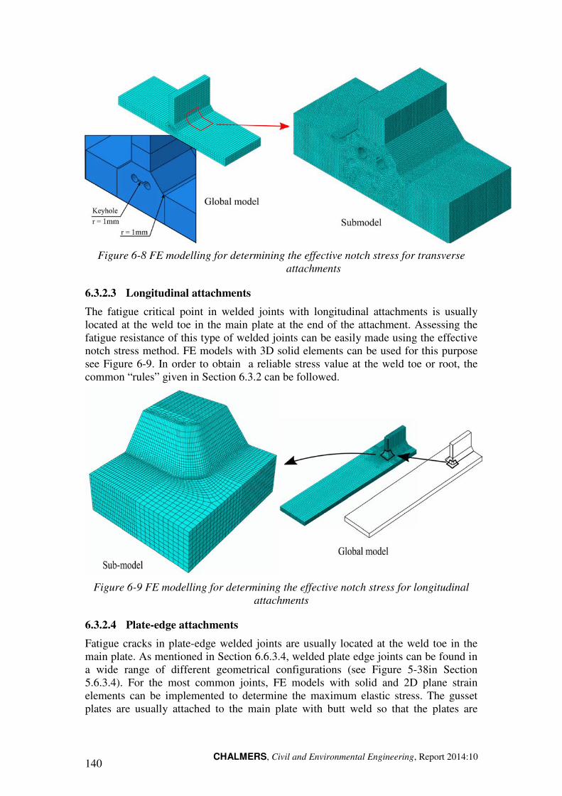
CHALMERS, Civil and Environmental Engineering, Report 2014:10 140
Figure 6-8 FE modelling for determining the effective notch stress for transverse attachments
6.3.2.3 Longitudinal attachments
The fatigue critical point in welded joints with longitudinal attachments is usually located at the weld toe in the main plate at the end of the attachment. Assessing the fatigue resistance of this type of welded joints can be easily made using the effective notch stress method. FE models with 3D solid elements can be used for this purpose see Figure 6-9. In order to obtain a reliable stress value at the weld toe or root, the common “rules” given in Section 6.3.2 can be followed.
Figure 6-9 FE modelling for determining the effective notch stress for longitudinal attachments
6.3.2.4 Plate-edge attachments
Fatigue cracks in plate-edge welded joints are usually located at the weld toe in the main plate. As mentioned in Section 6.6.3.4, welded plate edge joints can be found in a wide range of different geometrical configurations (see Figure 5-38in Section 5.6.3.4). For the most common joints, FE models with solid and 2D plane strain elements can be implemented to determine the maximum elastic stress. The gusset plates are usually attached to the main plate with butt weld so that the plates are
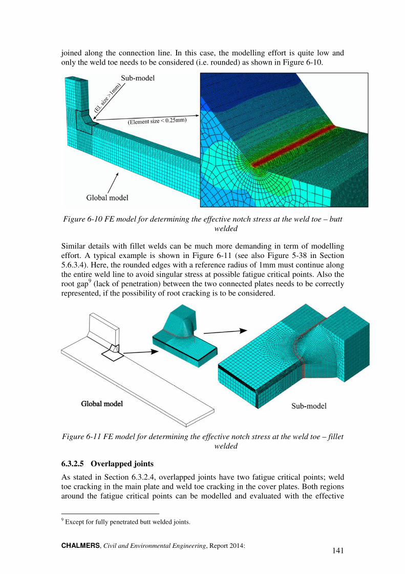
CHALMERS, Civil and Environmental Engineering, Report 2014: 141
joined along the connection line. In this case, the modelling effort is quite low and only the weld toe needs to be considered (i.e. rounded) as shown in Figure 6-10.
Figure 6-10 FE model for determining the effective notch stress at the weld toe – butt welded
Similar details with fillet welds can be much more demanding in term of modelling effort. A typical example is shown in Figure 6-11 (see also Figure 5-38 in Section 5.6.3.4). Here, the rounded edges with a reference radius of 1mm must continue along the entire weld line to avoid singular stress at possible fatigue critical points. Also the root gap9 (lack of penetration) between the two connected plates needs to be correctly represented, if the possibility of root cracking is to be considered.
Figure 6-11 FE model for determining the effective notch stress at the weld toe – fillet welded
6.3.2.5 Overlapped joints
As stated in Section 6.3.2.4, overlapped joints have two fatigue critical points; weld toe cracking in the main plate and weld toe cracking in the cover plates. Both regions around the fatigue critical points can be modelled and evaluated with the effective
9 Except for fully penetrated butt welded joints.
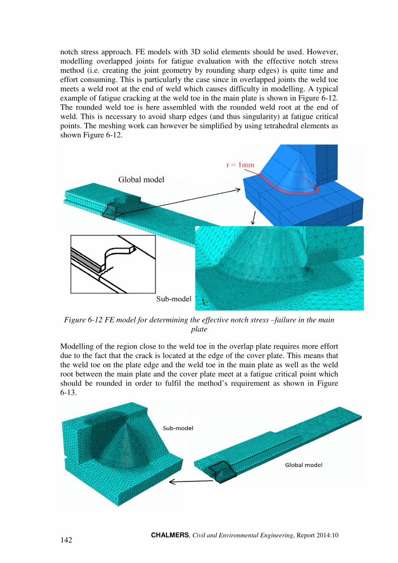
CHALMERS, Civil and Environmental Engineering, Report 2014:10 142
notch stress approach. FE models with 3D solid elements should be used. However, modelling overlapped joints for fatigue evaluation with the effective notch stress method (i.e. creating the joint geometry by rounding sharp edges) is quite time and effort consuming. This is particularly the case since in overlapped joints the weld toe meets a weld root at the end of weld which causes difficulty in modelling. A typical example of fatigue cracking at the weld toe in the main plate is shown in Figure 6-12. The rounded weld toe is here assembled with the rounded weld root at the end of weld. This is necessary to avoid sharp edges (and thus singularity) at fatigue critical points. The meshing work can however be simplified by using tetrahedral elements as shown Figure 6-12.
Figure 6-12 FE model for determining the effective notch stress –failure in the main plate
Modelling of the region close to the weld toe in the overlap plate requires more effort due to the fact that the crack is located at the edge of the cover plate. This means that the weld toe on the plate edge and the weld toe in the main plate as well as the weld root between the main plate and the cover plate meet at a fatigue critical point which should be rounded in order to fulfil the method’s requirement as shown in Figure 6-13.
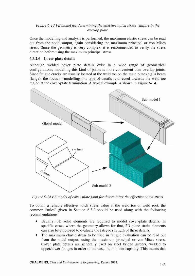
CHALMERS, Civil and Environmental Engineering, Report 2014: 143
Figure 6-13 FE model for determining the effective notch stress –failure in the overlap plate
Once the modelling and analysis is performed, the maximum elastic stress can be read out from the nodal output, again considering the maximum principal or von Mises stress. Since the geometry is very complex, it is recommended to verify the stress direction before using the maximum principal stress.
6.3.2.6 Cover plate details
Although welded cover plate details exist in a wide range of geometrical configurations, modelling this kind of joints is more convenient than overlap joints. Since fatigue cracks are usually located at the weld toe on the main plate (e.g. a beam flange), the focus in modelling this type of details is directed towards the weld toe region at the cover-plate termination. A typical example is shown in Figure 6-14.
Figure 6-14 FE model of cover plate joint for determining the effective notch stress
To obtain a reliable effective notch stress value at the weld toe or weld root, the common “rules” given in Section 6.3.2 should be used along with the following recommendations:
• Usually, 3D solid elements are required to model cover-plate details. In specific cases, where the geometry allows for that, 2D plane strain elements can also be employed to evaluate the fatigue strength of these details.
• The maximum elastic stress to be used in fatigue evaluation can be read out from the nodal output, using the maximum principal or von-Mises stress. Cover plate details are generally used on steel bridge girders, welded to upper/lower flanges in order to increase the moment capacity. This means that
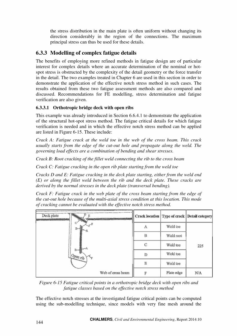
CHALMERS, Civil and Environmental Engineering, Report 2014:10 144
the stress distribution in the main plate is often uniform without changing its direction considerably in the region of the connections. The maximum principal stress can thus be used for these details.
6.3.3 Modelling of complex fatigue details
The benefits of employing more refined methods in fatigue design are of particular interest for complex details where an accurate determination of the nominal or hot-spot stress is obstructed by the complexity of the detail geometry or the force transfer in the detail. The two examples treated in Chapter 6 are used in this section in order to demonstrate the application of the effective notch stress method in such cases. The results obtained from these two fatigue assessment methods are also compared and discussed. Recommendations for FE modelling, stress determination and fatigue verification are also given.
6.3.3.1 Orthotropic bridge deck with open ribs
This example was already introduced in Section 6.6.4.1 to demonstrate the application of the structural hot-spot stress method. The fatigue critical details for which fatigue verification is needed and in which the effective notch stress method can be applied are listed in Figure 6-15. These include:
Crack A: Fatigue crack at the weld toe in the web of the cross beam. This crack usually starts from the edge of the cut-out hole and propagate along the weld. The governing load effects are a combination of bending and shear stresses.
Crack B: Root cracking of the fillet weld connecting the rib to the cross beam
Crack C: Fatigue cracking in the open rib plate starting from the weld toe
Cracks D and E: Fatigue cracking in the deck plate starting, either from the weld end (E) or along the fillet weld between the rib and the deck plate. These cracks are derived by the normal stresses in the deck plate (transversal bending).
Crack F: Fatigue crack in the web plate of the cross beam starting from the edge of the cut-out hole because of the multi-axial stress condition at this location. This mode of cracking cannot be evaluated with the effective notch stress method.
Figure 6-15 Fatigue critical points in a orthotropic bridge deck with open ribs and fatigue classes based on the effective notch stress method
The effective notch stresses at the investigated fatigue critical points can be computed using the sub-modelling technique, since models with very fine mesh around the
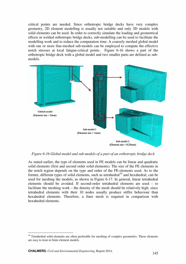
CHALMERS, Civil and Environmental Engineering, Report 2014: 145
critical points are needed. Since orthotropic bridge decks have very complex geometry, 2D element modelling is usually not suitable and only 3D models with solid elements can be used. In order to correctly simulate the loading and geometrical effects in welded orthotropic bridge decks, sub-modelling can be used to facilitate the modelling work and to reduce the computation time. A coarsely meshed global model with one or more fine-meshed sub-models can be employed to compute the effective notch stresses at local fatigue-critical points. Figure 6-16 shows a part of the orthotropic bridge deck with a global model and two smaller parts are defined as sub-models.
Figure 6-16 Global model and sub-models of a part of an orthotropic bridge deck
As stated earlier, the type of elements used in FE models can be linear and quadratic solid elements (first and second order solid elements). The size of the FE elements in the notch region depends on the type and order of the FE-elements used. As to the former, different types of solid elements, such as tetrahedral10 and hexahedral, can be used for meshing the models, as shown in Figure 6-17. In general, linear tetrahedral elements should be avoided. If second-order tetrahedral elements are used – to facilitate the meshing work – the density of the mesh should be relatively high, since tetrahedral elements with their 10 nodes usually produce stiffer behaviour than hexahedral elements. Therefore, a finer mesh is required in comparison with hexahedral elements.
10 Tetrahedral solid elements are often preferable for meshing of complex geometries. These elements are easy to treat in finite element models.
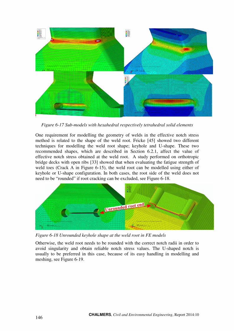
CHALMERS, Civil and Environmental Engineering, Report 2014:10 146
Figure 6-17 Sub-models with hexahedral respectively tetrahedral solid elements
One requirement for modelling the geometry of welds in the effective notch stress method is related to the shape of the weld root. Fricke [45] showed two different techniques for modelling the weld root shape; keyhole and U-shape. These two recommended shapes, which are described in Section 6.2.1, affect the value of effective notch stress obtained at the weld root. A study performed on orthotropic bridge decks with open ribs [33] showed that when evaluating the fatigue strength of weld toes (Crack A in Figure 6-15), the weld root can be modelled using either of keyhole or U-shape configuration. In both cases, the root side of the weld does not need to be “rounded” if root cracking can be excluded, see Figure 6-18.
Figure 6-18 Unrounded keyhole shape at the weld root in FE models
Otherwise, the weld root needs to be rounded with the correct notch radii in order to avoid singularity and obtain reliable notch stress values. The U-shaped notch is usually to be preferred in this case, because of its easy handling in modelling and meshing, see Figure 6-19.
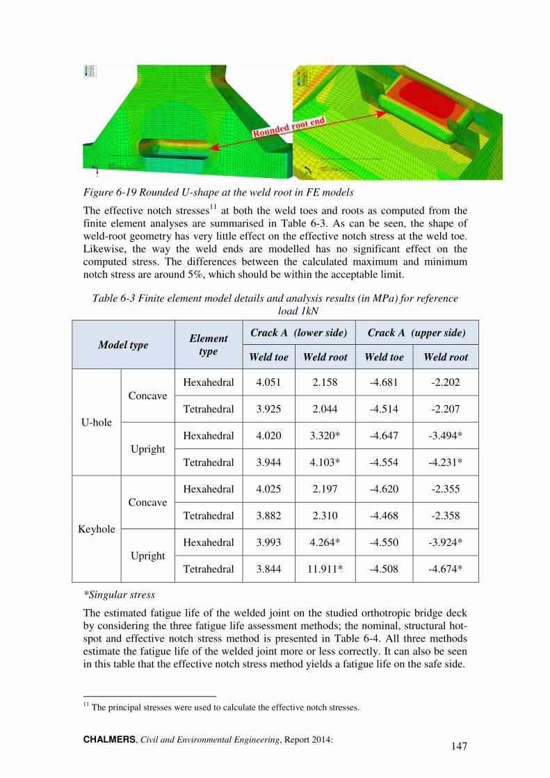
CHALMERS, Civil and Environmental Engineering, Report 2014: 147
Figure 6-19 Rounded U-shape at the weld root in FE models
The effective notch stresses11 at both the weld toes and roots as computed from the finite element analyses are summarised in Table 6-3. As can be seen, the shape of weld-root geometry has very little effect on the effective notch stress at the weld toe. Likewise, the way the weld ends are modelled has no significant effect on the computed stress. The differences between the calculated maximum and minimum notch stress are around 5%, which should be within the acceptable limit.
Table 6-3 Finite element model details and analysis results (in MPa) for reference load 1kN
Model type Element
type
Crack A (lower side) Crack A (upper side)
Weld toe Weld root Weld toe Weld root
U-hole
Concave Hexahedral 4.051 2.158 -4.681 -2.202
Tetrahedral 3.925 2.044 -4.514 -2.207
Upright Hexahedral 4.020 3.320* -4.647 -3.494*
Tetrahedral 3.944 4.103* -4.554 -4.231*
Keyhole
Concave Hexahedral 4.025 2.197 -4.620 -2.355
Tetrahedral 3.882 2.310 -4.468 -2.358
Upright Hexahedral 3.993 4.264* -4.550 -3.924*
Tetrahedral 3.844 11.911* -4.508 -4.674*
*Singular stress
The estimated fatigue life of the welded joint on the studied orthotropic bridge deck by considering the three fatigue life assessment methods; the nominal, structural hot-spot and effective notch stress method is presented in Table 6-4. All three methods estimate the fatigue life of the welded joint more or less correctly. It can also be seen in this table that the effective notch stress method yields a fatigue life on the safe side.
11 The principal stresses were used to calculate the effective notch stresses.
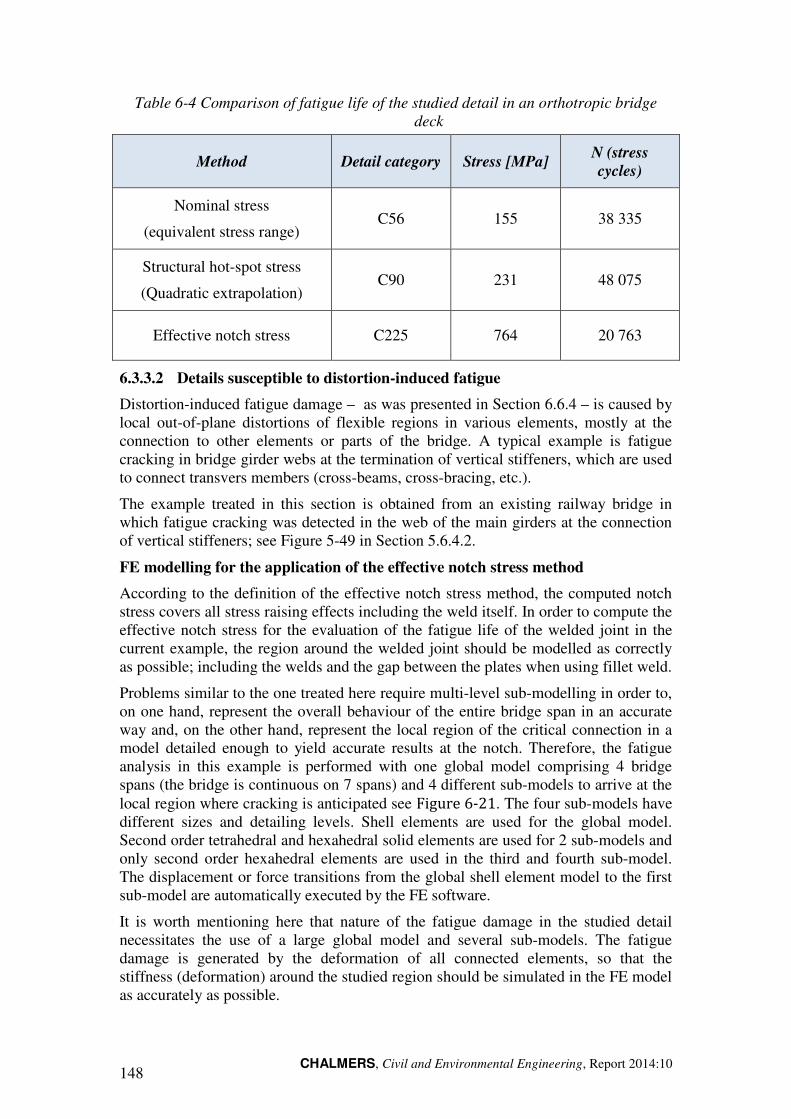
CHALMERS, Civil and Environmental Engineering, Report 2014:10 148
Table 6-4 Comparison of fatigue life of the studied detail in an orthotropic bridge deck
Method Detail category Stress [MPa] N (stress cycles)
Nominal stress
(equivalent stress range) C56 155 38 335
Structural hot-spot stress
(Quadratic extrapolation) C90 231 48 075
Effective notch stress C225 764 20 763
6.3.3.2 Details susceptible to distortion-induced fatigue
Distortion-induced fatigue damage – as was presented in Section 6.6.4 – is caused by local out-of-plane distortions of flexible regions in various elements, mostly at the connection to other elements or parts of the bridge. A typical example is fatigue cracking in bridge girder webs at the termination of vertical stiffeners, which are used to connect transvers members (cross-beams, cross-bracing, etc.).
The example treated in this section is obtained from an existing railway bridge in which fatigue cracking was detected in the web of the main girders at the connection of vertical stiffeners; see Figure 5-49 in Section 5.6.4.2.
FE modelling for the application of the effective notch stress method
According to the definition of the effective notch stress method, the computed notch stress covers all stress raising effects including the weld itself. In order to compute the effective notch stress for the evaluation of the fatigue life of the welded joint in the current example, the region around the welded joint should be modelled as correctly as possible; including the welds and the gap between the plates when using fillet weld.
Problems similar to the one treated here require multi-level sub-modelling in order to, on one hand, represent the overall behaviour of the entire bridge span in an accurate way and, on the other hand, represent the local region of the critical connection in a model detailed enough to yield accurate results at the notch. Therefore, the fatigue analysis in this example is performed with one global model comprising 4 bridge spans (the bridge is continuous on 7 spans) and 4 different sub-models to arrive at the local region where cracking is anticipated see Figure 6-21. The four sub-models have different sizes and detailing levels. Shell elements are used for the global model. Second order tetrahedral and hexahedral solid elements are used for 2 sub-models and only second order hexahedral elements are used in the third and fourth sub-model. The displacement or force transitions from the global shell element model to the first sub-model are automatically executed by the FE software.
It is worth mentioning here that nature of the fatigue damage in the studied detail necessitates the use of a large global model and several sub-models. The fatigue damage is generated by the deformation of all connected elements, so that the stiffness (deformation) around the studied region should be simulated in the FE model as accurately as possible.
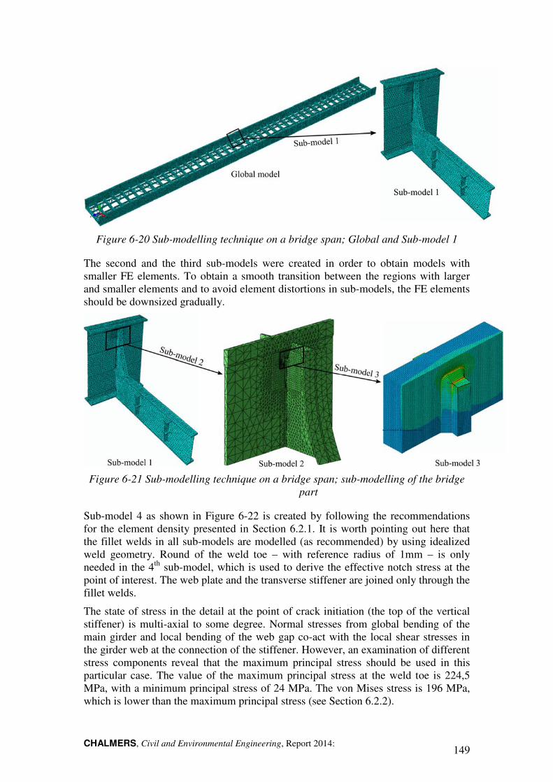
CHALMERS, Civil and Environmental Engineering, Report 2014: 149
Figure 6-20 Sub-modelling technique on a bridge span; Global and Sub-model 1
The second and the third sub-models were created in order to obtain models with smaller FE elements. To obtain a smooth transition between the regions with larger and smaller elements and to avoid element distortions in sub-models, the FE elements should be downsized gradually.
Figure 6-21 Sub-modelling technique on a bridge span; sub-modelling of the bridge part
Sub-model 4 as shown in Figure 6-22 is created by following the recommendations for the element density presented in Section 6.2.1. It is worth pointing out here that the fillet welds in all sub-models are modelled (as recommended) by using idealized weld geometry. Round of the weld toe – with reference radius of 1mm – is only needed in the 4th sub-model, which is used to derive the effective notch stress at the point of interest. The web plate and the transverse stiffener are joined only through the fillet welds.
The state of stress in the detail at the point of crack initiation (the top of the vertical stiffener) is multi-axial to some degree. Normal stresses from global bending of the main girder and local bending of the web gap co-act with the local shear stresses in the girder web at the connection of the stiffener. However, an examination of different stress components reveal that the maximum principal stress should be used in this particular case. The value of the maximum principal stress at the weld toe is 224,5 MPa, with a minimum principal stress of 24 MPa. The von Mises stress is 196 MPa, which is lower than the maximum principal stress (see Section 6.2.2).
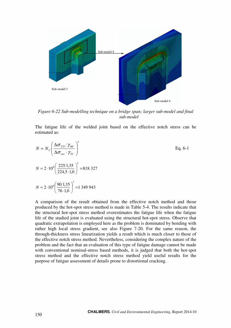
CHALMERS, Civil and Environmental Engineering, Report 2014:10 150
Figure 6-22 Sub-modelling technique on a bridge span; larger sub-model and final sub-model
The fatigue life of the welded joint based on the effective notch stress can be estimated as:
3
225
⋅∆
∆=
Ffens
MfCNN
γσ
γσ Eq. 6-1
3278180,15,224
35,1225102
3
6 =
⋅⋅=N
94334910,176
35,190102
3
6 =
⋅⋅=N
A comparison of the result obtained from the effective notch method and those produced by the hot-spot stress method is made in Table 5-4. The results indicate that the structural hot-spot stress method overestimates the fatigue life when the fatigue life of the studied joint is evaluated using the structural hot-spot stress. Observe that quadratic extrapolation is employed here as the problem is dominated by bending with rather high local stress gradient, see also Figure 7-20. For the same reason, the through-thickness stress linearization yields a result which is much closer to those of the effective notch stress method. Nevertheless, considering the complex nature of the problem and the fact that an evaluation of this type of fatigue damage cannot be made with conventional nominal-stress based methods, it is judged that both the hot-spot stress method and the effective notch stress method yield useful results for the purpose of fatigue assessment of details prone to distortional cracking.
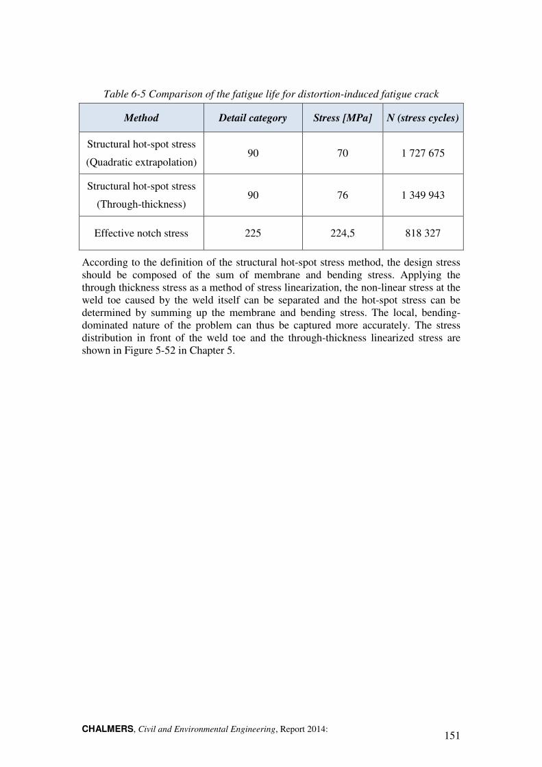
CHALMERS, Civil and Environmental Engineering, Report 2014: 151
Table 6-5 Comparison of the fatigue life for distortion-induced fatigue crack
Method Detail category Stress [MPa] N (stress cycles)
Structural hot-spot stress
(Quadratic extrapolation) 90 70 1 727 675
Structural hot-spot stress
(Through-thickness) 90 76 1 349 943
Effective notch stress 225 224,5 818 327
According to the definition of the structural hot-spot stress method, the design stress should be composed of the sum of membrane and bending stress. Applying the through thickness stress as a method of stress linearization, the non-linear stress at the weld toe caused by the weld itself can be separated and the hot-spot stress can be determined by summing up the membrane and bending stress. The local, bending-dominated nature of the problem can thus be captured more accurately. The stress distribution in front of the weld toe and the through-thickness linearized stress are shown in Figure 5-52 in Chapter 5.

CHALMERS, Civil and Environmental Engineering, Report 2014:10 152
CHALMERS, Civil and Environmental Engineering, Report 2014: 153
7 References
1. Schijve, J., Fatigue of structures and materials. 2009: Springer Netherlands. 456.
2. Croce, P., Background to fatigue load models for Eurocode 1: Part 2 Traffic Loads. Progress in Structural Engineering and Materials, 2001. 3(4): p. 335-345.
3. Sedlacek, G., et al., Background document to EN 1991- Part 2 - Traffic loads for road bridges - and consequences for the design, in JRC Scientific and Technical Reports. 2008, JRC European commission.
4. Kühn, B., et al., Assessment of Existing Steel Structures: Recommmendations for Estimation of Remaining Fatigue Life, G. Sedlacek, et al., Editors. 2008.
5. Nussbaumer, A., L. Borges, and L. Davaine, Fatigue Design of Steel and Composite Structures. ECCS Eurocode Design Manuals. 2011, ECCS: ECCS – European Convention for Constructional Steelwork. 311.
6. Croce, P., et al., Guidebook 2 - Design of Bridges, ed. P. Croce. 2010, Praque: Czech Technical University.
7. Sanpaolesi, L. and P. Croce, eds. Handbook 4 - Design of bridges. Leonardo Da Vinci Pilot Project CZ/02/B/F/pp-134007. 2005: Pisa, Italy.
8. Calgaro, J.A., M. Tschumi, and H. Gulvanessian, Designers’ Guide to Eurocode 1: Action on bridges, ed. H. Gulvanessian. 2010, Chippenham, UK.: Antony Rowe Limited.
9. 1993-2, E., Eurocode 3: Design of Steel Structures - Part 2: Steel Bridges 2006, European committee for Standardization: Brussels.
10. Nussbaumer, A., European standard for fatigue design of steel structures and perspectives, in International Conference on Fatigue and Fracture in the Infrastructure. 2006.
11. EN 1993-2 Eurocode 3: Design of Steel Structures - Part 2: Steel Bridges 2006, European committee for Standardization: Brussels.
12. Marshall, P.W. and J. Wardenier. Tubular versus Non-Tubular Hot Spot Stress Methods. in Proceedings of The Fifteenth (2005) International Offshore and Polar Engineering Conference. 2005. Seoul, Korea: The International Society of Offshore and Polar Engineers.
13. Radaj, D., C.M. Sonsino, and W. Fricke, Fatigue Assessment of Welded Joints by Local Approaches. 2. Ed. 2006: Woodhead Publishing, Cambridge.
14. Niemi, E., Stress determination for Fatigue Analysis of Welded Components, in IIW doc. IIS/IIW-1221-93. 1995, The International Institute of Welding: Cambridge, England.
15. Al-Emrani, M., Fatigue-critical details in steel bridges (in Swedish). 2006, Department of Structural Engineering, Chalmers University of Technology: Report 2006:7
CHALMERS, Civil and Environmental Engineering, Report 2014:10 154
16. Fricke, W., et al., Comparative fatigue strength assessment of a structural detail in a containership using various approaches of classification societies. Marine structures, 2002. Vol. 15(1): p. pp.1-13.
17. Hobbacher, A., Recommendation for fatigue design of welded joints and components, in IIW-1823-07 ex. XIII-2151r4-07/XV-1254r4-07. 2008, The international Institute of Welding: Cambridge, England.
18. EN 1993-1-9. Eurocode 3: Design of Steel Structures - Part 1-9: Fatigue. 2005: CEN, Brussels.
19. Wernicke, R., Fatigue strength assessment of cruciform joints with misalignment, in Doc. IIW-1872-01. 2001, The international Institute of Welding: Cambridge, England.
20. Fricke, W., Recommended Hot Spot Analysis Procedure for Structural Details of FPSO’s and Ships Based on Round-Robin FE Analyses. International Journal of Offshore and Polar Engineering, 2001. Vol. 12(No. 1): p. pp.1-8.
21. Storsul, R., E. Landet, and I. Lotsberg, Convergence Analysis for Welded Details in Ship Shaped Structures, in Proceedings of OMAE-FPSO 2004 OMAE Specialty Symposium on FPSO Integrity, OMAE-FPSO'04-0016, Editor. 2004: Houston, USA.
22. EN 1090-2. Execution of steel structures and aluminium structures - Part 2:Technical requirement for steel structures. 2008: CEN, Brussels.
23. ISO 5817, Welding — Fusion-welded joints in steel, nickel, titanium and their alloys (beam welding excluded) — Quality levels for imperfections. 2005, International Organization for Standardization: Geneva, Switzerland.
24. Dong, P., A structural stress definition and numerical implementation for fatigue analysis of welded joints. International Journal of Fatigue, 2001. 23(10): p. 865-876.
25. Dong, P. and J.K. Hong, Analysis of hot spot stress and alternative structural stress methods. The 22nd international conference on offshore mechanics and artic engineering, 2003. 3: p. 213-224.
26. Dong, P., J.K. Hong, and Z. Cao, Structural stress based master S-N curve for welded joints, in IIW Doc. XIII -1930-02/XV-1119-02. 2002, 55th Annual Assembly of International Institute of Welding: Copenhagen, Denmark. p. pp. 24.
27. Xiao, Z.-G. and K. Yamada, A method of determining geometric stress for fatigue strength evaluation of steel welded joints. International Journal of Fatigue, 2004. 26(12): p. 1277-1293.
28. Radaj, D., Assessment of fatigue strength of welded structures based on local parameters. VTT symposium 157 fatigue design, 1995. 3: p. 349-366.
29. Kyuba, H. and P. Dong, Equilibrium-equivalent structural stress approach to fatigue analysis of a rectangular hollow section joint. International Journal of Fatigue, 2005. 27(1): p. 85-94.
30. Noh, B., J. Song, and S. Bae, Fatigue Strength evaluation of the Load-Carrying Cruciform Fillet Welded Joints Using Hot-Spot Stress. Key Engineering Materials, 2006. Vols.324-325: p. pp. 1281-1284.

CHALMERS, Civil and Environmental Engineering, Report 2014: 155
31. Fricke, W., A. Kahl, and H. Paetzold, Fatigue Assessment of Root Cracking of Fillet Welds Subjected to Throat bending Using the Structural Stress Approach, in IIW document XIII-2072-05/XV-1198-05. 2005, The International Institute of Welding: Germany.
32. Eriksson, Å., et al., Weld evaluation using FEM - A guide to fatigue-loaded structures. 2003, Gothenburg, Sweden: Industrilitteratur AB.
33. Aygül, M., M. Al-Emrani, and S. Urushadze, Modelling and fatigue life assessment of orthotropic bridge deck details using FEM. International Journal of Fatigue, 2012. 40(0): p. 129-142.
34. Aygül, M., et al., Evaluation of the fatigue strength of an orthotropic bridge deck detail using hot spot stress approach, in 63rd Annual Assembly & International Conference of the International Institute of Welding. 2010, AWST-10/63: Istanbul, Turkey. p. 261-268.
35. Fayard, J., A. Bignonnet, and K. Dang Van, Fatigue Design Criterion For Welded Structures. Fatigue & Fracture of Engineering Materials & Structures, 1996. 19(6): p. 723-729.
36. Aygül, M., et al., A comparative study of different fatigue failure assessments of welded bridge details. International Journal of Fatigue, 2013. 49(0): p. 62-72.
37. Miki, C. and K. Tateishi, Fatigue strength of cope hole details in steel bridges. International Journal of Fatigue, 1997. 19(6): p. 445-455.
38. Aygül, M., et al., A comparative study of different fatigue failure assessments of welded bridge details. International Journal of Fatigue, 2013. 49(0): p. 62-72.
39. DNV-RP-203 Fatigue Design of Offshore Steel Structures. 2011, Det Norske Veritas - Offshore Codes: Norway.
40. Zhang, G. and B. Richter, New approach to the numerical fatigue-life prediction of spot-welded structures. Fatigue and Fracture of Engineering Materials and Structures, 2000. 23(6): p. 499-508.
41. Sonsino, C.M., et al., Notch stress concepts for the fatigue assessment of welded joints - Background and applications. International Journal of Fatigue, 2012. 34(1): p. 2-16.
42. Sonsino, C.M., A consideration of allowable equivalent stresses for fatigue design of welded joints according to the notch stress concept with the reference radii rref = 1.00 and 0.05 mm. Welding in the World, 2009. 53(3-4).
43. Radaj, D., C.M. Sonsino, and W. Fricke, Recent developments in local concepts of fatigue assessment of welded joints. International Journal of Fatigue, 2009. 31(1): p. 2-11.
44. IIW, Guideline for the Fatigue Assessment by Notch Stress Analysis for Welded Structures, W. Fricke, Editor. 2010, IIW Doc. XIII-2240-08/XV-1289-08, International Institute of welding.
45. Fricke, W., Guideline for the fatigue assessment by notch stress analysis for welded structures. The International Institute of Welding, 2008. IIW Doc.
XIII-2240-08/XV-1289-08(IIW Doc. XIII-2240-08/XV-1289-08).

CHALMERS, Civil and Environmental Engineering, Report 2014:10 156

CHALMERS, Civil and Environmental Engineering, Report 2014: 157