Fast parallelizable scenario-based stochasticoptimization

Ajay K. Sampathirao∗, Pantelis Sopasakis∗,Alberto Bemporad∗, Panos Patrinos∗∗

∗ IMT School for Advanced Studies Lucca, Italy,∗∗ ESAT, KU Leuven, Belgium.

September 14, 2016

I. Stochastic Optimal Control

Stochastic Optimal Control

Optimisation problem:

V ?(p) = minπ=ukk=N−1

k=0

E

[Vf (xN , ξN ) +

N−1∑k=0

`k(xk, uk, ξk)

],

s.t x0 = p,

xk+1 = Aξkxk +Bξkuk + wξk ,

where:

I At time k we measure xk and ξk−1I E[·]: conditional expectation wrt the product probability measure

I Casual policy uk = ψk(p,ξξξk−1), with ξξξk = (ξ0, ξ1, . . . , ξk)

I ` and Vf can encode constraints

Sampathirao et al., 2015, 2016.

Stochastic Optimal Control

Optimisation problem:

V ?(p) = minπ=ukk=N−1

k=0

E

[Vf (xN , ξN ) +

N−1∑k=0

`k(xk, uk, ξk)

],

s.t x0 = p,

xk+1 = Aξkxk +Bξkuk + wξk ,

where:

I At time k we measure xk and ξk−1

I E[·]: conditional expectation wrt the product probability measure

I Casual policy uk = ψk(p,ξξξk−1), with ξξξk = (ξ0, ξ1, . . . , ξk)

I ` and Vf can encode constraints

Sampathirao et al., 2015, 2016.

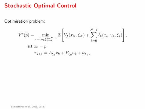
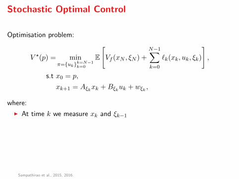
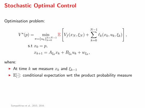
Stochastic Optimal Control

Optimisation problem:

V ?(p) = minπ=ukk=N−1

k=0

E

[Vf (xN , ξN ) +

N−1∑k=0

`k(xk, uk, ξk)

],

s.t x0 = p,

xk+1 = Aξkxk +Bξkuk + wξk ,

where:

I At time k we measure xk and ξk−1I E[·]: conditional expectation wrt the product probability measure

I Casual policy uk = ψk(p,ξξξk−1), with ξξξk = (ξ0, ξ1, . . . , ξk)

I ` and Vf can encode constraints

Sampathirao et al., 2015, 2016.

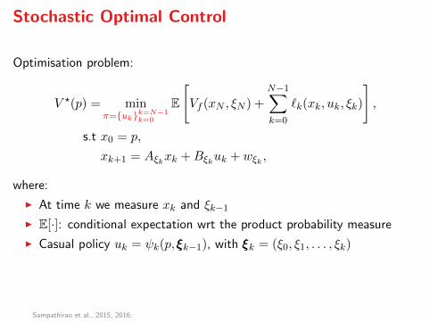
Stochastic Optimal Control

Optimisation problem:

V ?(p) = minπ=ukk=N−1

k=0

E

[Vf (xN , ξN ) +

N−1∑k=0

`k(xk, uk, ξk)

],

s.t x0 = p,

xk+1 = Aξkxk +Bξkuk + wξk ,

where:

I At time k we measure xk and ξk−1I E[·]: conditional expectation wrt the product probability measure

I Casual policy uk = ψk(p,ξξξk−1), with ξξξk = (ξ0, ξ1, . . . , ξk)

I ` and Vf can encode constraints

Sampathirao et al., 2015, 2016.

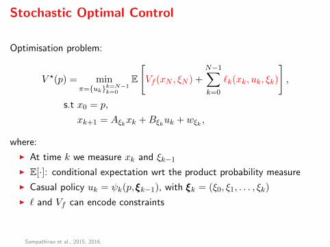
Stochastic Optimal Control

Optimisation problem:

V ?(p) = minπ=ukk=N−1

k=0

E

[Vf (xN , ξN ) +

N−1∑k=0

`k(xk, uk, ξk)

],

s.t x0 = p,

xk+1 = Aξkxk +Bξkuk + wξk ,

where:

I At time k we measure xk and ξk−1I E[·]: conditional expectation wrt the product probability measure

I Casual policy uk = ψk(p,ξξξk−1), with ξξξk = (ξ0, ξ1, . . . , ξk)

I ` and Vf can encode constraints

Sampathirao et al., 2015, 2016.

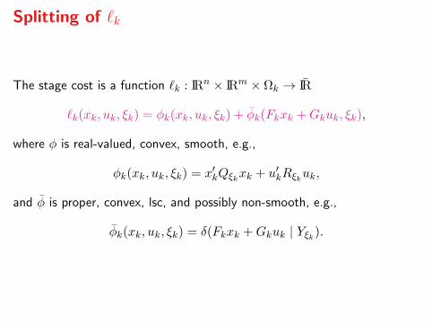
Splitting of `k

The stage cost is a function `k : IRn × IRm × Ωk → IR

`k(xk, uk, ξk) = φk(xk, uk, ξk) + φk(Fkxk +Gkuk, ξk),

where φ is real-valued, convex, smooth, e.g.,

φk(xk, uk, ξk) = x′kQξkxk + u′kRξkuk,

and φ is proper, convex, lsc, and possibly non-smooth, e.g.,

φk(xk, uk, ξk) = δ(Fkxk +Gkuk | Yξk).

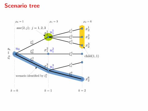
Scenario tree

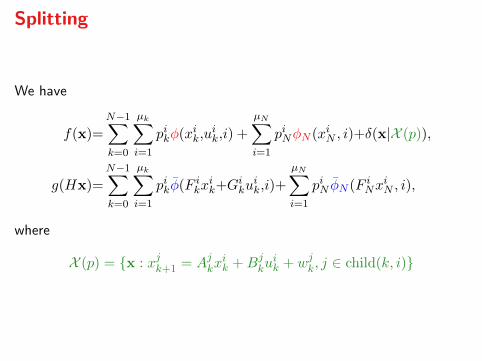
Splitting

We have

f(x)=

N−1∑k=0

µk∑i=1

pikφ(xik,uik,i) +

µN∑i=1

piNφN (xiN , i)+δ(x|X (p)),

g(Hx)=

N−1∑k=0

µk∑i=1

pikφ(F ikxik+G

iku

ik,i)+

µN∑i=1

piN φN (F iNxiN , i),

where

X (p) = x : xjk+1 = Ajkxik +Bj

kuik + wjk, j ∈ child(k, i)

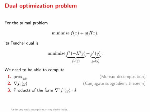
Dual optimization problem

For the primal problem

minimize f(x) + g(Hx),

its Fenchel dual is

minimize f∗(−H ′y)︸ ︷︷ ︸f(y)

+ g∗(y)︸ ︷︷ ︸g(y)

.

We need to be able to compute

1. proxγg (Moreau decomposition)

2. ∇f(y) (Conjugate subgradient theorem)

3. Products of the form ∇2f(y) · d

Under very weak assumptions, strong duality holds.

II. The Forward-BackwardLine-Search Algorithm

Problem statement

minimize ϕ(x) := f(x) + g(x)

I f , g closed proper convex

I f : IRn → IR is L-smooth

f(z) ≤ Qf1/L(z;x) := f(x) + 〈∇f(x), z − x〉+ L2 ‖z − x‖

2, ∀x, z

I g : IRn → IR ∪ +∞ has easily computable proximal mapping

proxγg(x) = arg minz∈IRn

g(z) + 1

2γ ‖z − x‖2

Parikh & Boyd, 2014.

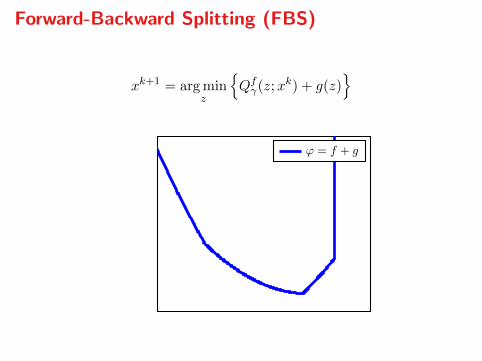
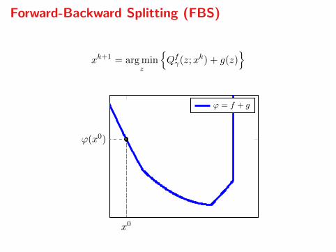
Forward-Backward Splitting (FBS)

xk+1 = arg minz

Qfγ(z;xk) + g(z)

x0

ϕ(x0)

ϕ = f + g

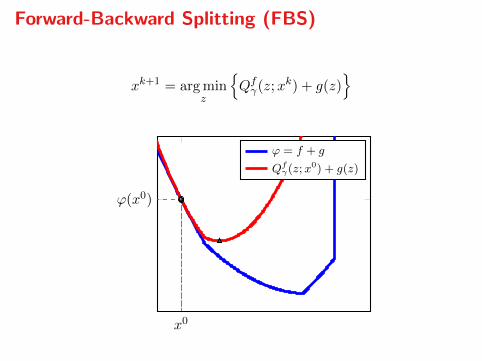
Forward-Backward Splitting (FBS)

xk+1 = arg minz

Qfγ(z;xk) + g(z)

x0

ϕ(x0)

ϕ = f + g

Forward-Backward Splitting (FBS)

xk+1 = arg minz

Qfγ(z;xk) + g(z)

x0

ϕ(x0)

ϕ = f + g

Qfγ(z;x

0) + g(z)

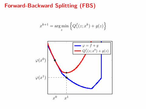
Forward-Backward Splitting (FBS)

xk+1 = arg minz

Qfγ(z;xk) + g(z)

x0 x1

ϕ(x0)

ϕ(x1)

ϕ = f + g

Qfγ(z;x

0) + g(z)

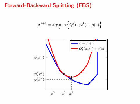
Forward-Backward Splitting (FBS)

xk+1 = arg minz

Qfγ(z;xk) + g(z)

x0 x1 x2

ϕ(x0)

ϕ(x1)

ϕ(x2)

ϕ = f + g

Qfγ(z;x

1) + g(z)

Forward-Backward Splitting (FBS)

xk+1 = arg minz

Qfγ(z;xk) + g(z)

x0 x1 x2 x3

ϕ(x0)

ϕ(x1)

ϕ(x2)ϕ(x3)

ϕ = f + g

Qfγ(z;x

2) + g(z)

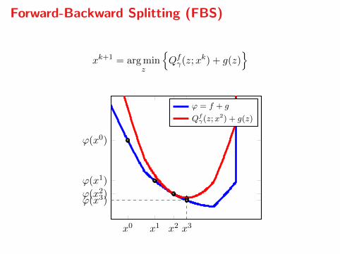
Forward-Backward Splitting (FBS)

The basic FBS algorithm is

xk+1 = proxγg(xk − γ∇f(xk))

which is a fixed point iteration for

x = proxγg(x− γ∇f(x)).

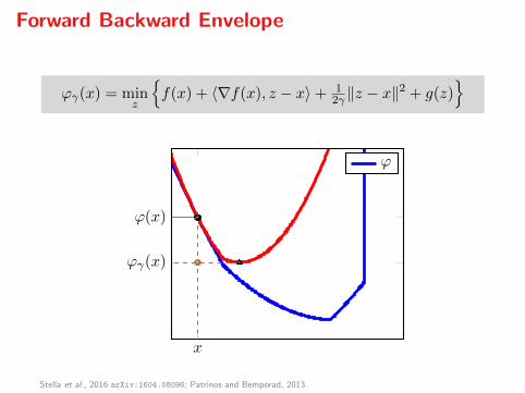
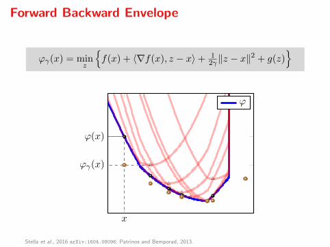
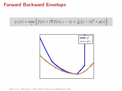
Forward Backward Envelope

ϕγ(x) = minz

f(x) + 〈∇f(x), z − x〉+ 1

2γ ‖z − x‖2 + g(z)

x

ϕ(x)

ϕγ(x)

ϕ

Stella et al., 2016 arXiv:1604.08096; Patrinos and Bemporad, 2013.

Forward Backward Envelope

ϕγ(x) = minz

f(x) + 〈∇f(x), z − x〉+ 1

2γ ‖z − x‖2 + g(z)

x

ϕ(x)

ϕγ(x)

ϕ

Stella et al., 2016 arXiv:1604.08096; Patrinos and Bemporad, 2013.

Forward Backward Envelope

ϕγ(x) = minz

f(x) + 〈∇f(x), z − x〉+ 1

2γ ‖z − x‖2 + g(z)

x

ϕ(x)

ϕγ(x)

ϕϕγ

Stella et al., 2016 arXiv:1604.08096; Patrinos and Bemporad, 2013.

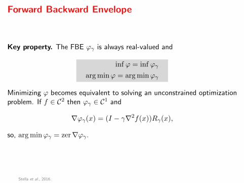
Forward Backward Envelope

Key property. The FBE ϕγ is always real-valued and

inf ϕ = inf ϕγ

arg minϕ = arg minϕγ

Minimizing ϕ becomes equivalent to solving an unconstrained optimizationproblem. If f ∈ C2 then ϕγ ∈ C1 and

∇ϕγ(x) = (I − γ∇2f(x))Rγ(x),

so, arg minϕγ = zer∇ϕγ .

Stella et al., 2016.

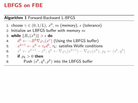
LBFGS on FBE

Algorithm 1 Forward-Backward L-BFGS

1: choose γ ∈ (0, 1/L), x0, m (memory), ε (tolerance)2: Initialize an LBFGS buffer with memory m3: while ‖Rγ(xk)‖ > ε do4: dk ← −Bk∇ϕγ(xν) (Using the LBFGS buffer)5: xk+1 ← xk + τkd

k, τk: satisfies Wolfe conditions6: sk ← xk+1 − xk, qk ← ∇ϕγ(xk+1)−∇ϕγ(xk), ρk ← 〈sk, qk〉7: if ρk > 0 then8: Push (sk, qk, ρk) into the LBFGS buffer

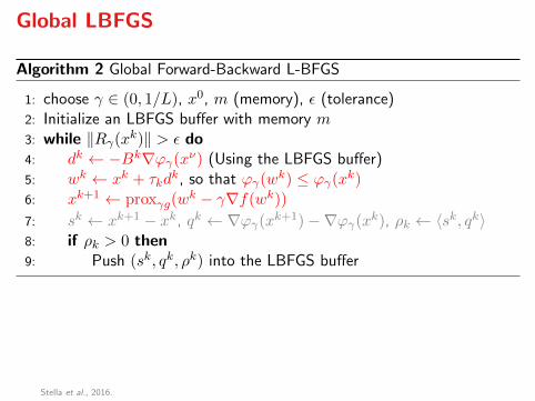
Global LBFGS

Algorithm 2 Global Forward-Backward L-BFGS

1: choose γ ∈ (0, 1/L), x0, m (memory), ε (tolerance)2: Initialize an LBFGS buffer with memory m3: while ‖Rγ(xk)‖ > ε do4: dk ← −Bk∇ϕγ(xν) (Using the LBFGS buffer)5: wk ← xk + τkd

k, so that ϕγ(wk) ≤ ϕγ(xk)6: xk+1 ← proxγg(w

k − γ∇f(wk))

7: sk ← xk+1 − xk, qk ← ∇ϕγ(xk+1)−∇ϕγ(xk), ρk ← 〈sk, qk〉8: if ρk > 0 then9: Push (sk, qk, ρk) into the LBFGS buffer

Stella et al., 2016.

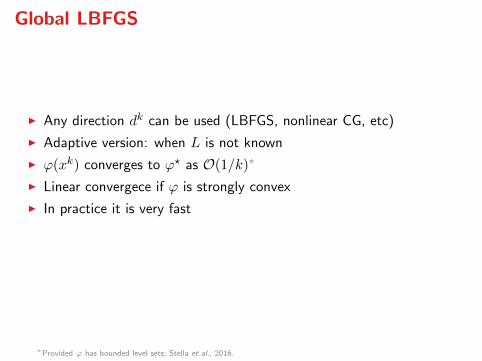
Global LBFGS

I Any direction dk can be used (LBFGS, nonlinear CG, etc)

I Adaptive version: when L is not known

I ϕ(xk) converges to ϕ? as O(1/k)∗

I Linear convergece if ϕ is strongly convex

I In practice it is very fast

∗Provided ϕ has bounded level sets; Stella et al., 2016.

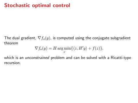
Stochastic optimal control

The dual gradient, ∇fo(y), is computed using the conjugate subgradienttheorem

∇fo(y) = H arg minz〈z,H ′y〉+ f(z),

which is an unconstrained problem and can be solved with a Ricatti-typerecursion.

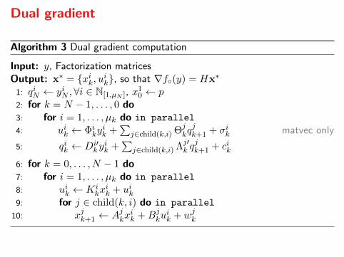
Dual gradient

Algorithm 3 Dual gradient computation

Input: y, Factorization matricesOutput: x∗ = xik, uik, so that ∇f(y) = Hx∗

1: qiN ← yiN ,∀i ∈ N[1,µN ], x10 ← p

2: for k = N − 1, . . . , 0 do3: for i = 1, . . . , µk do in parallel

4: uik ← Φikyik +

∑j∈child(k,i) Θj

kqjk+1 + σik matvec only

5: qik ← Di′ky

ik +

∑j∈child(k,i) Λj′k q

jk+1 + cik

6: for k = 0, . . . , N − 1 do7: for i = 1, . . . , µk do in parallel

8: uik ← Kikx

ik + uik

9: for j ∈ child(k, i) do in parallel

10: xjk+1 ← Ajkxik +Bj

kuik + wjk

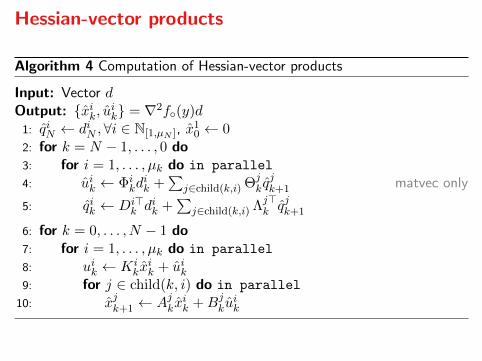
Hessian-vector products

Algorithm 4 Computation of Hessian-vector products

Input: Vector dOutput: xik, uik = ∇2f(y)d1: qiN ← diN ,∀i ∈ N[1,µN ], x

10 ← 0

2: for k = N − 1, . . . , 0 do3: for i = 1, . . . , µk do in parallel

4: uik ← Φikdik +

∑j∈child(k,i) Θj

kqjk+1 matvec only

5: qik ← Di>k dik +

∑j∈child(k,i) Λj>k qjk+1

6: for k = 0, . . . , N − 1 do7: for i = 1, . . . , µk do in parallel

8: uik ← Kikx

ik + uik

9: for j ∈ child(k, i) do in parallel

10: xjk+1 ← Ajkxik +Bj

kuik

III. Results

Implementation

I Implementation on NVIDIA Tesla 2075

I Mass-spring system

I 10 states, 20 inputs, N = 15

I Binary scenario tree

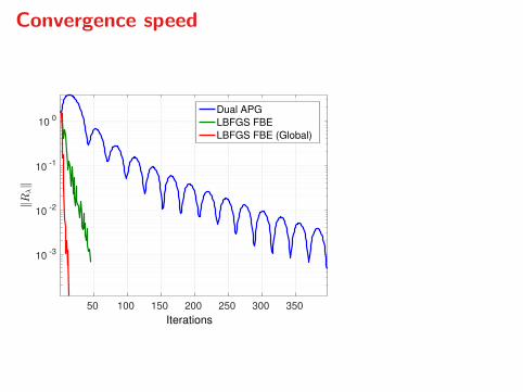
Convergence speed

50 100 150 200 250 300 350

Iterations

10-3

10-2

10-1

100

‖Rλ‖

Dual APG

LBFGS FBE

LBFGS FBE (Global)

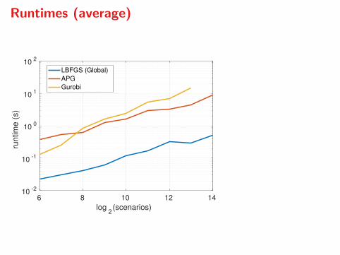
Runtimes (average)

6 8 10 12 14

log2(scenarios)

10-2

10-1

100

101

102

runtim

e (

s)

LBFGS (Global)

APG

Gurobi

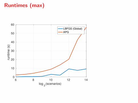
Runtimes (max)

6 8 10 12 14

log2(scenarios)

0

10

20

30

40

50

60

runtim

e (

s)

LBFGS (Global)

APG

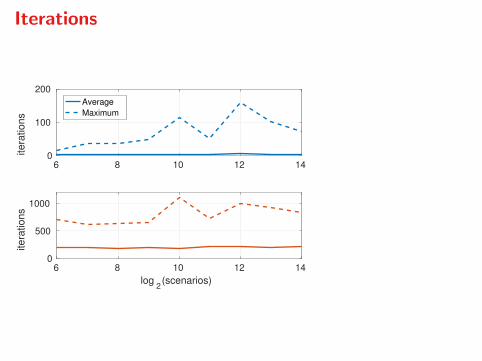
Iterations

6 8 10 12 140

100

200

ite

ratio

ns

Average

Maximum

6 8 10 12 14

log2(scenarios)

0

500

1000

ite

ratio

ns

References

1. A.K. Sampathirao, P. Sopasakis, A. Bemporad and P. Patrinos, “Proximalquasi-Newton methods for scenario-based stochastic optimal control,” IFAC 2017,submitted.

2. A.K. Sampathirao, P. Sopasakis, A. Bemporad and P. Patrinos, “Stochasticpredictive control of drinking water networks: large-scale optimisation and GPUs,”IEEE CST (prov. accepted), arXiv:1604.01074

3. A.K. Sampathirao, P. Sopasakis, A. Bemporad and P. Patrinos, “Distributedsolution of stochastic optimal control problems on GPUs,” in Proc. 54th IEEEConf. on Decision and Control, Osaka, Japan, 2015, pp. 7183–7188.

4. L. Stella, A. Themelis and P. Patrinos, “Forward-backward quasi-Newton methodsfor nonsmooth optimization problems,” arXiv:1604.08096, 2016.

5. P. Patrinos and A. Bemporad, “Proximal Newton methods for convex compositeoptimization,” IEEE CDC 2013.

6. N. Parikh and S. Boyd, “Proximal Algorithms,” Foundations and Trends inOptimization, 1(3), pp. 123–231, 2014.

7. J. Nocedal and S. Wright, “Numerical Optimization,” Springer, 2006.

Thank you for your attention.