FaST linear mixed models for genome -wide association … we use only one SNP at a time in our work,...

Nature Methods

FaST linear mixed models for genome-wide association studies

Christoph Lippert, Jennifer Listgarten, Ying Liu, Carl M Kadie, Robert I Davidson & David Heckerman

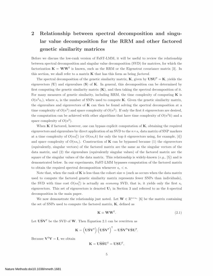
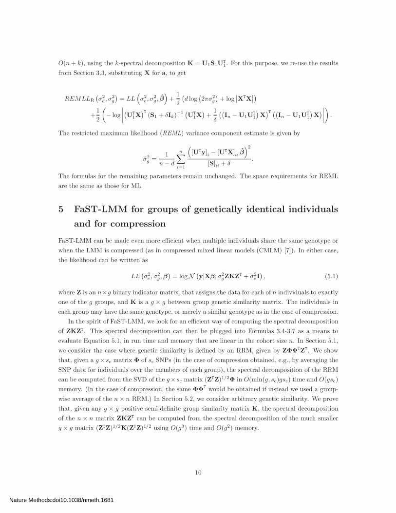
Supplementary Figure 1 Q-Q plots for the WTCCC data.

Supplementary Note 1 The FaST-LMM algorithm.

Supplementary Note 2 Null-model contamination.

Nature Methods:doi10.1038/nmeth.1681

Supplementary Figure 1

0 2 4 6 80

1

2

3

4

5

6

7

8

expected negative log P values

obse

rved

neg

ativ

e lo

g P

val

ues

ATTFaST−LMM 4KFaST−LMM 8KFaST−LMM complete

Q-Q plots for the WTCCC data. Shown are observed versus expected negative log P values for

the association analyses on the CD phenotype described in the main paper. We used FaST-LMM

to test all SNPs on chromosome 1, and SNP sets of various sizes from all but this chromosome—the

complete set (340K), 8K, and 4K—to compute the RRM. We also used ATT to compute P values.

1


Supplementary Note 1: The FaST-LMM Algorithm

Here we describe our approach called FaST-LMM, which stands for Factored Spectrally Transformed

Linear Mixed Models. We derive formulas that allow for efficient evaluation of the likelihood as well

as the maximum likelihood (ML) and restricted maximum likelihood (REML) parameters. We con-

sider the cases where the genetic similarity matrix has full and low rank separately. The following

notation will be used.

• n denotes the cohort size (the number of individuals represented in the data set).

• s denotes the total number of SNPs to be tested.

• d denotes the number of fixed effects in a single model, including the offset, the covariates,

and in the case of an alternative model, the SNP to be tested. Although we use only one SNP

at a time in our work, all equations follow regardless of the number of SNPs fixed effects.

• k denotes the rank of the genetic similarity matrix.

• sc denotes the number of SNPs used to construct the genetic similarity matrix.

• X ∈ Rn×d denotes the matrix of fixed effects. This matrix includes the column of 1s corre-

sponding to the offset, the covariates, and the SNP to be tested.

• y ∈ Rn×1 denotes the vector of phenotype measurements.

• K ∈ Rn×n denotes the symmetric positive (semi)-definite genetic similarity matrix.

• Ia denotes the identity matrix of dimension a. If no subscript a is given, the dimensionality is

implied by the context.

• σ2g denotes the magnitude of the genetic variance.

• σ2e denotes the magnitude of the residual variance.

• δ ≡ σ2

e

σ2g

denotes the fraction of genetic variance and residual variance.

• β ∈ Rd×1 denotes the vector of fixed effect weights corresponding to X ∈ R

n×d.

• S ∈ Rn×n denotes the diagonal matrix containing the eigenvalues of K ordered by their

magnitude from large to small as diagonal elements.

• U ∈ Rn×n denotes to the matrix of eigenvectors of K, in the order of the corresponding

eigenvalues.

• USUT = K is the spectral decomposition of K.

• |A| denotes the determinant of matrix A.

• AT denotes the transpose of matrix A.

1


• A−1 denotes the inverse of matrix A.

• A−T denotes the transposed inverse (or inverse of the transpose) of matrix A.

• [A]ij denotes the element of matrix A in the ith row and jth column.

• [A]i: denotes the ith row of matrix A.

• [a]i denotes the ith entry of vector a.

• 0 denotes a matrix where every entry is zero.

• [A,B] denotes the concatenation of matrices A and B.

1 LMMs with a full rank genetic similarity

We first consider the case where the genetic similarity matrix is of full rank (i.e., the rank is equal

to the cohort size).

1.1 Linear-time evaluation of the log likelihood

The log likelihood is parameterized by a weight vector β and the variances of the random components,

σ2e and σ2

g :

LL(

σ2

e , σ2

g , β)

= logN(

y|Xβ; σ2

gK + σ2

eI)

. (1.1)

Introducing δ ≡σ2

e

σ2g

, the covariance matrix becomes σ2g (K + δI), and the likelihood becomes a

function of β, δ and σ2g [1]:

LL(

δ, σ2

g , β)

= logN(

y|Xβ; σ2

g (K + δI))

.

Using the formula for the n-variate Normal distribution, we obtain

LL(

δ, σ2

g , β)

= −1

2

(

n log(

2πσ2

g

)

+ log (|(K + δI)|) +1

σ2g

(y − Xβ)T(K + δI)

−1(y − Xβ)

)

. (1.2)

Letting USUT = K be the spectral decomposition of K, and noting that I = UUT, Equation 1.2

becomes

LL(

δ, σ2

g , β)

= −

1

2

(

n log(

2πσ2

g

)

+ log(∣

∣

(

USUT + δUU

T)∣

∣

)

+1

σ2g

(y −Xβ)T(

USUT + δUU

T)

−1

(y − Xβ)

)

.

Next, we factor out U and UT from the covariance of the Normal, so that it becomes the diagonal

matrix (S + δI), obtaining

−1

2

(

n log(

2πσ2

g

)

+ log(∣

∣U (S + δI)UT∣

∣

)

+1

σ2g

(y − Xβ)T(

U (S + δI)UT)

−1(y − Xβ)

)

. (1.3)

The determinant of the genetic similarity matrix, |U (S + δI)UT| can be written as |(S + δI)| using

the properties that |AB| = |A||B|, and that |U| = |UT| = 1. The inverse of the genetic similarity

2


matrix can be rewritten as U (S + δI)−1

UT using the properties that (AB)−1 = B−1A−1, that

U−1 = UT, and that U−T = U. Thus, after additionally moving out U from the covariance term so

that it now acts as a rotation matrix on the inputs (X) and targets (y), we obtain

−1

2

(

n log(

2πσ2

g

)

+ log(

|U| |(S + δI)|∣

∣UT∣

∣

)

+1

σ2g

(y − Xβ)T U (S + δI)−1UT (y − Xβ)

)

= −1

2

(

n log(

2πσ2

g

)

+ log (|(S + δI)|) +1

σ2g

((

UTy)

−(

UTX)

β)T

(S + δI)−1((

UTy)

−(

UTX)

β)

)

.

(1.4)

The “Fa” in FaST-LMM gets its name from these factorizations. As the covariance matrix of the

Normal distribution is now a diagonal matrix (S + δI), the log likelihood can be rewritten as the

sum over n terms, yielding

−1

2

(

n log(

2πσ2

g

)

+

n∑

i=1

log ([S]ii + δ) +1

σ2g

n∑

i=1

([UTy]i − [UTX]i: β)2

[S]ii + δ

)

. (1.5)

Note that this expression is equal to the product of n single-variate Normal distributions, on the

data transformed by UT, yielding the equation

LL(

δ, σ2

g , β)

= logn∏

i=1

N([

UTy]

i|[

UTX]

i:β; σ2

g([S]ii + δ)

).

Having pre-computed the spectral decomposition of K, we can rotate the phenotype and all

SNPs once to get UX and Uy. Given the parameters δ, σ2g and β each evaluation of the likelihood

is now linear in the cohort size n, as compared to cubic for direct evaluation of Equation 1.1.

1.2 Finding the maximum likelihood fixed effect weights efficiently

We take the gradient of the log likelihood in Equation 1.4 with respect to β and set it to zero, giving

0 =1

σ2g

(

(

UTX)T

(S + δI)−1(

UTy)

−(

UTX)T

(S + δI)−1(

UTX)

β)

.

Multiplying both sides by σ2g and then bringing the part involving β to one side, we get

(

UTX)T

(S + δI)−1(

UTX)

β =(

UTX)T

(S + δI)−1(

UTy)

.

Multiplying both sides by the inverse of the factor on the left side, we obtain

β =[

(

UTX)T

(S + δI)−1(

UTX)

]

−1(

UTX)T

(S + δI)−1(

UTy)

.

As (S + δI) is a diagonal matrix, the matrix products again can be written as a sum over n inde-

pendent terms, yielding

β =

[

n∑

i=1

1

[S]ii + δ

[

UTX]T

i:

[

UTX]

i:

]

−1 [ n∑

i=1

1

[S]ii + δ

[

UTX]T

i:

[

UTy]

i

]

,

analogous to linear regression estimates for β on the rotated data. Assuming that all the terms

involving the spectral decomposition of K are precomputed, this equation can be evaluated in O(n).

3


1.3 Finding the maximum likelihood genetic variance efficiently

We start by substituting β from the previous section into the log likelihood, Equation 1.5, and set

the derivative with respect to σ2g to zero, giving

0 = −1

2

n

σ2g

−1

σ4g

n∑

i=1

(

[UTy]i − [UTX]i: β)2

[S]ii + δ

.

Multiplying both sides by 2σ4g and solving for σ2

g , we get

σ2

g =1

n

n∑

i=1

(


[S]ii + δ.

This equation also can be evaluated in O(n).

1.4 Efficient evaluation of the maximum likelihood

Plugging in σ2g and β into Equation 1.5, the log likelihood becomes a function only of δ,

LL(δ, σ2g(δ), β(δ)) = LL(δ):

LL(δ) = −1

2

n log (2π) +

n∑

i=1

log ([S]ii + δ) + n + n log1

n

n∑

i=1

(

[UTy]i − [UTX]i: β(δ))2

[S]ii + δ

.

As described next, we optimize this function of δ using a one-dimensional numerical optimizer to find

the maximum likelihood value of δ, from which the maximum likelihood values of all the parameters

can be directly computed.

1.5 Optimization of δ

As we’ve just shown, finding the maximum log likelihood of our model (LL(

σ2e , σ2

g , β)

) is equivalent

to finding the value of δ that maximizes LL(δ), a non-convex optimization problem. To avoid local

maxima in FaST-LMM, a quasi-exhaustive one dimensional optimization scheme similar to the one

proposed in [1] is applied. In order to bracket local minima, we evaluate the maximum of the log

likelihood for 100 equidistant values of log(δ), ranging -10 to 10. Then, we apply Brent’s method (a

1D numerical optimization algorithm) to find the locally optimal δ in each bracket where the middle

log likelihood is higher than the log likelihoods of the neighboring evaluations.

To speed-up a full GWAS scan, one can find the maximum likelihood setting for δ for just the

null-model, re-using the same δ for all alternative models. This speedup was described in [2] and is

used in all of our experiments unless otherwise noted.

4


2 Relationship between spectral decomposition and singu-

lar value decomposition for the RRM and other factored

genetic similarity matrices

Before we discuss the low-rank version of FaST-LMM, it will be useful to review the relationship

between spectral decomposition and singular value decomposition (SVD) for matrices, for which the

factorization K = WWT is known, such as the RRM or the Eigenstrat covariance matrix [3]. In

this section, we shall refer to a matrix K that has this form as being factored.

The spectral decomposition of the genetic similarity matrix, K, given by USUT = K, yields the

eigenvectors (U) and eigenvalues (S) of K. In general, this decomposition can be determined by

first computing the genetic similarity matrix (K), and then taking the spectral decomposition of it.

For many measures of genetic similarity, including RRM, the time complexity of computing K is

O(n2sc), where sc is the number of SNPs used to compute K. Given the genetic similarity matrix,

the eigenvalues and eigenvectors of K can then be found solving the spectral decomposition at a

time complexity of O(n3) and space complexity of O(n2). If only the first k eigenvectors are desired,

the computation can be achieved with other algorithms that have time complexity of O(n2k) and a

space complexity of O(n2).

When K if factored, however, one can bypass explicit computation of K, obtaining the required

eigenvectors and eigenvalues by direct application of an SVD to the n×sc data matrix of SNP markers

at a time complexity of O(ns2c) (or O(nsck) for only the top k eigenvectors using, for example, [4])

and space complexity of O(nsc). Construction of K can be bypassed because (1) the eigenvectors

(equivalently, singular vectors) of the factored matrix are the same as the singular vectors of the

data matrix, and (2) the eigenvalues (equivalently singular values) of the factored matrix are the

square of the singular values of the data matrix. This relationship is widely-known (e.g., [5]) and is

demonstrated below. In our experiments, FaST-LMM bypasses computation of the factored matrix

to obtain the required spectral decomposition whenever sc < n.

Note that, when the rank of K is less than the cohort size n (such as occurs when the data matrix

used to compute the factored genetic similarity matrix represents fewer SNPs than individuals),

the SVD with time cost O(ns2c) is actually an economy SVD, that is, it yields only the first sc

eigenvectors. This set of eigenvectors is denoted U1 in Section 3 and referred to as the k-spectral

decomposition in the main paper.

We now demonstrate the relationship just noted. Let W ∈ Rn×sc [6] be the matrix containing

the set of SNPs used to compute the factored matrix, K, defined as

K ≡ WWT. (2.1)

Let USVT be the SVD of W. Then Equation 2.1 can be rewritten as

K =(

USVT

)(

USVT

)T

= USVTVSUT.

Because VTV = I, we obtain

K = USSUT = USUT,

5


where Sii ≡ SiiSii. By definition, U consists of the eigenvectors of K (because it satisfies the

properties of a spectral decomposition of K, namely that K = USUT where S is diagonal and U

contains orthonormal vectors). Furthermore, the eigenvalues of K are given by S2

ii. Consequently,

we can obtain the spectral decomposition of K by computing the SVD of W, which has time cost

O(ns2c).

3 LMMs with a low rank genetic similarity matrix

Now we consider the evaluation of the likelihood when the rank of K, k, is low (k < n) (i.e., K is

not full rank). This condition will occur when the RRM is used and the number of SNPs used to

estimate it, sc = k, is smaller than n. It will also occur if we reduce the rank of K to k ≤ min(n, sc)

by eliminating the eigenvectors with the lowest eigenvalues as described in Discussion of the main

paper. We address both possibilities in this section.

Let USUT = K be the complete spectral decomposition of K. Thus, S is an n × n diagonal

matrix containing the k non-zero eigenvalues on the top-left of the diagonal, followed by n− k zeros

on the bottom-right, and U is an n×n matrix of eigenvectors. Now, write the full n×n orthonormal

matrix U as U ≡ [U1,U2], where U1 ∈ Rn×k contains the eigenvectors corresponding to non-zero

eigenvalues, and U2 ∈ Rn×n−k contains the eigenvectors corresponding to zero eigenvalues. Thus,

we have

K = USUT = [U1,U2]

[

S1 0

0 S2

]

[U1,U2]T = U1S1U

T

1+ U2S2U

T

2.

As S2 = [0], K can be recovered by the k-spectral decomposition of K:

K = U1S1UT

1.

The expression (K + δI), however, is always of full rank (because δ > 0):

K + δI = U (S + δI)UT = U

[

S1 + δIk 0

0 δIn−k

]

UT.

Therefore, it is not possible to simply ignore U2 while using our previous approach (as in in Sec-

tion 1), as U2 enters the expression for the log likelihood. Furthermore, directly computing the

complete spectral decomposition does not exploit the low rank of K. Thus, we use algebraic ma-

nipulations to rewrite the likelihood in terms not involving U2, as explained next. As a result, we

incur only the computational complexity of computing U1 rather than U.

3.1 Linear time evaluation of the likelihood

To exploit the low rank of K to evaluate the log likelihood efficiently, one possible approach would

be to augment the spectrum using n − k vectors that are orthogonal to the first k. Unfortunately,

this strategy has a time complexity of O((n−k)n2). Consequently, we take the following alternative

approach.

6


We begin with Equation 1.2:

LL(δ, σ2

g, β) = −1

2

(

n log(

2πσ2

g

)

+ log |(K + δI)| +1

σ2g


−1(y − Xβ)

)

.

The two terms involving K+δI are highlighted in color and will be treated separately in the following.

As in Equation 1.5, the log-determinant of the genetic similarity matrix can be efficiently com-

puted using the economy SVD of X to obtain the spectral decomposition of K:

log |(K + δI)| =

n∑

i=1

log ([S]ii + δ) =

k∑

i=1

log ([S]ii + δ) + (n − k) (log δ), (3.1)

where we use the fact that the last n − k singular values are zero.

Also, as we show in Section 3.3, the residual quadratic form can be evaluated using the low-rank

decomposition:

(y − Xβ)T (K + δI)−1 (y − Xβ) =(

UT

1y − UT

1Xβ)T

(S1 + δIk)−1(

UT

1y − UT

1Xβ)

+1

δ

((

In − U1UT

1

)

y −(

In − U1UT

1

)

Xβ)T ((

In − U1UT

1

)

y −(

In − U1UT

1

)

Xβ)

. (3.2)

Furthermore, both terms in the expression on the right can be written as sums, leading to


−1(y − Xβ) =

k∑

i=1

([UT

1y]i − [UT

1X]i: β)2

[S]ii + δ+

1

δ

n∑

i=1

([

y − U1

(

UT

1y)]

i−[

X − U1

(

UT

1X)]

iβ)2

. (3.3)

3.2 Finding the maximum likelihood and parameters efficiently

Plugging both the determinant (Equation 3.1) and the quadratic form (Equation 3.3) into the log

likelihood, we obtain

LL(δ, σ2

g , β) = −

1

2

(

n log(

2πσ2

g

)

+k∑

i=1

log(

[S]ii

+ δ)

+ (n − k) (log δ)

)

−

1

2σ2g

(

k∑

i=1

([

UT

1y]

i−

[

UT

1X]

i:β)

2

[S]ii

+ δ+

1

δ

n∑

i=1

([

y − U1

(

UT

1y)]

i−

[

X − U1

(

UT

1X)]

iβ)2

)

. (3.4)

Setting the gradient of LL(δ, σ2g, β) in Equation 3.4 with respect to β to zero, we obtain

β =

[(

k∑

i=1

1

[S]ii + δ

[

UT

1X]T

i:

[

UT

1X]

i:

)

+

(

1

δ

n∑

i=1

[(

I− U1UT

1

)

X]T

i:

[(

I − U1UT

1

)

X]

i:

)]−1

∗

[(

k∑

i=1

1

[S]ii + δ

[

UT

1X]T

i:

[

UT

1y]

i

)

+

(

1

δ

n∑

i=1

[(

I− U1UT

1

)

X]T

i:

[(

I − U1UT

1

)

y]

i

)]

. (3.5)

7


Plugging β into the log likelihood and setting the derivative with respect to σ2g to zero, we get

0 = −

1

2

n

σ2g

−

1

σ4g

k∑

i=1

(

[

UT

1y]

i−

[

UT

1X]

i:β)

2

[S]ii

+ δ+

1

δ

n∑

i=1

(

[(

I− U1UT

1

)

y]

i−

[(

I− U1UT

1

)

X]

i:β)

2

.

Consequently,

σ2

g =1

n

k∑

i=1

(

[UT

1y]i − [UT

1X]i: β

)2

[S]ii + δ+

1

δ

n∑

i=1

(

[(

I − U1UT

1

)

y]

i−[(

I − U1UT

1

)

X]

i:β)2

. (3.6)

Plugging Equations 3.5 and 3.6 into 3.4 yields

LL(δ, σ2

g , β) = −

1

2

(

n log (2π) +k∑

i=1

log(

[S]ii

+ δ)

+ (n − k) (log δ)

)

−

1

2

n + n log

1

n

k∑

i=1

(

[

UT

1y]

i−

[

UT

1X]

i:β)2

[S]ii

+ δ+

1

δ

n∑

i=1

(

[

y − U1

(

UT

1y)]

i−

[

X −U1

(

UT

1X)]

iβ)

2

,

(3.7)

which can be evaluated in O(n + k).

3.3 Derivation of the low-rank quadratic form

Let K be a rank k genetic similarity matrix whose spectral decomposition can be written

K = USUT = U1S1UT

1 + U2S2UT

2 = U1S1UT

1 + U2 [0]UT

2 = U1S1UT

1,

where

U = [U1,U2] , (3.8)

U1 ∈ Rn×k contains the eigenvectors corresponding to non-zero eigenvalues, and U2 ∈ R

n×n−k.

Using the fact that U ∈ Rn×n is a normal matrix, that is, U−1 = UT, we have

In = UUT = [U1,U2] [U1,U2]T

= U1UT

1 + U2UT

2. (3.9)

Solving Equation 3.9 for U2UT

2, we get

U2UT

2= In − U1U

T

1. (3.10)

Further, because the columns of U are orthonormal, it follows that

In = UTU,

Ik = UT

1U1,

8


In−k = UT

2U2. (3.11)

Let a ≡ (y − Xβ). Our goal is to efficiently evaluate aT (K + δI)−1

a. Substituting the spectral

decomposition for K into this expression, we have

aT (K + δI)−1

a =(

UTa)

T

(S + δI)−1(

UTa)

. (3.12)

Using Equation 3.8, we can stack the matrix product in blocks involving U1 and U2 to re-write this

expression as[

UT

1a UT

2a]T

[

(S1 + δIk)−1

0

0 (δIn−k)−1

]

[

UT

1a UT

2a]

. (3.13)

As the off-diagonal blocks of the central matrix are equal to zero, the quadratic form reduces to the

sum of two terms, namely

(

UT

1a)T

(S1 + δIk)−1(

UT

1a)

+(

UT

2a)T

(δIn−k)−1(

UT

2a)

. (3.14)

Substituting UT

2U2 for In−k (using Equation 3.11), the second term becomes

(

UT

2a)T

(δIn−k)−1(

UT

2a)

=1

δaTU2In−kU

T

2a =1

δaTU2

(

UT

2U2

)

UT

2a. (3.15)

Finally, using Equation 3.10, we can eliminate U2 to obtain

1

δ

(

U2UT

2a)T (

U2UT

2a)

=1

δ

((

In − U1UT

1

)

a)T ((

In − U1UT

1

)

a)

. (3.16)

Substituting (3.16) into (3.14), we obtain

aT (K + δI)−1a =

(

UT

1a)T

(S1 + δIk)−1(

UT

1a)

+1

δ

((

In − U1UT

1

)

a)T ((

In − U1UT

1

)

a)

. (3.17)

Substituting (y − Xβ) for a, we obtain Equation 3.2.

4 Restricted maximum likelihood

So far the derivations have been limited to maximum likelihood parameter estimation. However, it

is straightforward to extend these results to the restricted log likelihood, which comprises the log

likelihood (with β plugged in), plus three additional terms [1]:

REMLLR

(

σ2

e , σ2

g

)

= LL(

σ2

e , σ2

g , β)

+1

2

(

d log(

2πσ2

g

)

+ log∣

∣XTX∣

∣− log∣

∣

∣XT (K + δI)

−1X

∣

∣

∣

)

.

Again, using the spectral decomposition of K, the restricted log likelihood becomes

REMLLR

(

σ2

e , σ2

g

)

= LL(

σ2

e , σ2

g , β)

+1

2

(

d log(

2πσ2

g

)

+ log∣

∣XTX∣

∣

− log∣

∣

∣

(

UTX)T

(S + δI)−1(

UTX)

∣

∣

∣

)

.

Neglecting the cubic dependence on d for computing the determinants, these additional terms can

be evaluated in time complexity O(n). If K has rank k < n, we can evaluate the additional terms in

9


O(n + k), using the k-spectral decomposition K = U1S1UT

1. For this purpose, we re-use the results

from Section 3.3, substituting X for a, to get

REMLLR

(

σ2

e , σ2

g

)

= LL(

σ2

e , σ2

g , β)

+1

2

(

d log(

2πσ2

g

)

+ log∣

∣XTX∣

∣

)

+1

2

(

− log

∣

∣

∣

∣

(

UT

1X)T

(S1 + δIk)−1(

UT

1X)

+1

δ

((

In − U1UT

1

)

X)T ((

In − U1UT

1

)

X)

∣

∣

∣

∣

)

.

The restricted maximum likelihood (REML) variance component estimate is given by

σ2

g =1

n − d

n∑

i=1

(


[S]ii + δ.

The formulas for the remaining parameters remain unchanged. The space requirements for REML

are the same as those for ML.

5 FaST-LMM for groups of genetically identical individuals

and for compression

FaST-LMM can be made even more efficient when multiple individuals share the same genotype or

when the LMM is compressed (as in compressed mixed linear models (CMLM) [7]). In either case,

the likelihood can be written as

LL(

σ2

e , σ2

g , β)

= logN(

y|Xβ; σ2

gZKZT + σ2

eI)

, (5.1)

where Z is an n×g binary indicator matrix, that assigns the data for each of n individuals to exactly

one of the g groups, and K is a g × g between group genetic similarity matrix. The individuals in

each group may have the same genotype, or merely a similar genotype as in the case of compression.

In the spirit of FaST-LMM, we look for an efficient way of computing the spectral decomposition

of ZKZT. This spectral decomposition can then be plugged into Formulas 3.4-3.7 as a means to

evaluate Equation 5.1, in run time and memory that are linear in the cohort size n. In Section 5.1,

we consider the case where genetic similarity is defined by an RRM, given by ZΦΦTZT. We show

that, given a g× sc matrix Φ of sc SNPs (in the case of compression obtained, e.g., by averaging the

SNP data for individuals over the members of each group), the spectral decomposition of the RRM

can be computed from the SVD of the g×sc matrix (ZTZ)1/2Φ in O(min(g, sc)gsc) time and O(gsc)

memory. (In the case of compression, the same ΦΦT would be obtained if instead we used a group-

wise average of the n × n RRM.) In Section 5.2, we consider arbitrary genetic similarity. We prove

that, given any g × g positive semi-definite group similarity matrix K, the spectral decomposition

of the n × n matrix ZKZT can be computed from the spectral decomposition of the much smaller

g × g matrix (ZTZ)1/2K(ZTZ)1/2 using O(g3) time and O(g2) memory.

10


5.1 Spectral decomposition of ZΦΦTZT

Let Φ be the g × sc matrix of SNP data. Let Z be the n × g group indicator matrix that assigns

data for each of n individuals to exactly one group. Then the genetic similarity matrix becomes

ZΦΦTZT.

For our argument, we use the fact that, given a matrix A, both AAT as well as ATA share the

same eigenvalues, and that these eigenvalues are given by the square of the singular values of A.

The eigenvectors of AAT are given by the left singular vectors of A; and the eigenvectors of ATA

are given by the right singular vectors of A. So the eigenvalues of ZΦΦTZT are the same as the

eigenvalues of ΦTZTZΦ = ΦT(ZTZ)1/2(ZTZ)1/2Φ. Using the same argument, the latter matrix has

the same eigenvalues as (ZTZ)1/2ΦΦT(ZTZ)1/2. These eigenvalues are given by the square of the

singular values of (ZTZ)1/2Φ, where (ZTZ)1/2 is a g × g diagonal matrix holding the square root of

the number of members of each group on the diagonal. Because (ZTZ)1/2 is diagonal, multiplication

can be done in O(gsc) time.

Let USVT be the SVD of (ZTZ)1/2Φ. Then the following holds:

ZΦΦTZT = Z(ZTZ)−1/2(ZTZ)1/2ΦΦT(ZTZ)1/2(ZTZ)−1/2ZT, (5.2)

where (ZTZ)−1/2 is a g × g diagonal matrix, holding one over the square root of the number of

members of each group on its diagonal. Substituting (ZTZ)1/2Φ by its SVD, we get

Z(ZTZ)−1/2USVTVSUT(ZTZ)−1/2ZT.

Finally, by orthonormality of V, this expression simplifies to

Z(ZTZ)−1/2USUT(ZTZ)−1/2ZT, (5.3)

where S = S2 is a diagonal matrix, holding the non-zero eigenvalues of ΦΦT on its diagonal. The

columns of Z(ZTZ)−1/2U are orthonormal, as can be seen by

UT(ZTZ)−1/2ZTZ(ZTZ)−1/2U = UT(ZTZ)(ZTZ)−1U = UTU = Ig. (5.4)

where we have once again used the fact that (ZTZ) is diagonal. It follows that Z(ZTZ)−1/2U holds

the eigenvectors of ZΦΦTZT, completing the spectral decomposition of ZΦΦTZ. Note that the

rotation of the data by (Z(ZTZ)−1/2U)T can be done efficiently by multiplying the data by the

transpose of the rows of (ZTZ)−1/2U belonging to the respective group.

5.2 Spectral decomposition of ZKZT, when the factors are not known

Here we extend the arguments in Section 5.1 to any positive semi-definite g × g group genetic simi-

larity matrix K. In this case, the spectral decomposition of ZKZT = USUT can also be computed

efficiently, namely from the spectral decomposition of (ZTZ)1/2K(ZTZ)1/2 = USUT, which can be

computed in O(g3) run time. As K is positive semi-definite, there always exists some square root

Φ of K, such that K = ΦΦT. In Section 5.1, we have shown, that ZKZT and (ZTZ)1/2K(ZTZ)1/2

have the same eigenvalues. Consequently, we can compute the eigenvalues S of ZKZT from the

spectral decomposition USUT. Analogous to the derivation in Equations 5.2-5.3, it follows that the

eigenvectors of ZKZT are Z(ZTZ)−1/2U, where by Equation 5.4, the columns are orthonormal.

11


References

[1] Kang, H. M. et al. Efficient control of population structure in model organism association

mapping. Genetics 107 (2008).

[2] Kang, H. M. et al. Variance component model to account for sample structure in genome-wide

association studies. Nat. Genet. 42, 348–354 (2010).

[3] Price, A. L. et al. Principal components analysis corrects for stratification in genome-wide

association studies. Nature genetics 38, 904–909 (2006).

[4] Tipping, M. & Bishop, C. M. Probabilistic principal component analysis. J.R. Statistical Society,

Series B 61, 6111–622 (1999).

[5] Wall, M. E., Rechtsteiner, A. & Rocha, L. M. A Practical Approach to Microarray Data Analysis

(Kluwer, Norwell, MA, 2003).

[6] Yang, J. et al. Common SNPs explain a large proportion of the heritability for human height.

Nat. Genet. 42, 565–569 (2010).

[7] Zhang, Z. et al. Mixed linear model approach adapted for genome-wide association studies. Nat.

Genet. 42, 355–360 (2010).

12


Supplementary Note 2: Null-Model Contamination

In our experiments measuring the accuracy of association P values in the main paper, the SNPs

being tested and the SNPs used to estimate genetic similarity were deliberately made disjoint. Here,

we discuss the reason for this approach.

As discussed in the main paper, a LMM with no fixed effects using an RRM constructed from a

set of SNPs is equivalent to a linear regression of the SNPs on the phenotype, with linear weights

(i.e., SNP effects) integrated over independent Normal distributions having the same variance [1].

So, by using a LMM with an RRM to test a given SNP for an association with the phenotype, we

are in effect adjusting for background SNPs, precisely those used to construct the RMM. Thus, when

testing a given SNP, using that SNP in the computation of the RRM would be equivalent to using

that SNP as a regressor in the null model, making the log likelihood of the null-model higher than it

should be, thus making the P value higher than it should be. We call this phenomenon null-model

contamination. A weaker form of this phenomenon could exist due to linkage disequilibrium.

In this note, we show that, on the WTCCC data for the CD phenotype with non-white individuals

and close family members included, this effect produces substantially deflated P values as measured

by the λ statistic, and quantify the degree to which LD plays a role. In an ideal experiment, we

would compare the λ statistic for two association tests of each available SNP, one where the RRM

is constructed from all SNPs, and one where the RRM is constructed from all SNPs but the SNP

being tested (and those nearby having at least a certain amount of LD with it). Unfortunately, such

a comparison is computationally infeasible, as it would require the construction of many thousands

of RRMs and their corresponding spectral decompositions.

Instead, we used an approach where the SNPs used to construct the RRM were chosen to be

systematically further and further away from a set of test SNPs, while holding the number of SNPs

used to construct the RRM (i.e., the number of background SNPs in the equivalent linear regression)

constant. In particular, after ordering SNPs by their position, we used every thirty-second SNP

starting from the ith SNP in each chromosome to form a set of test SNPs. In addition, we created

six sets of SNPs to construct RRMs, each set lying further away from the set of test SNPs. In a

given set, we included every thirty-second SNP starting at the i + jth SNP in each chromosome,

j = 0, 1, 2, 4, 8, and 16. This experiment was performed for i = 1, 2, 3, 4, and 5. Each set of SNPs

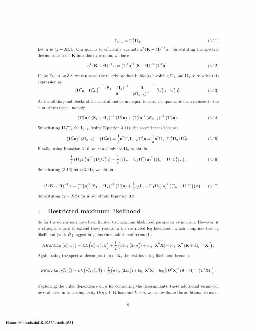
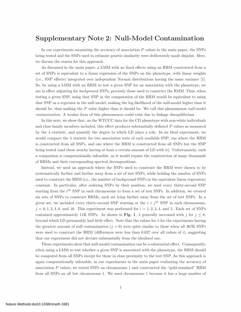
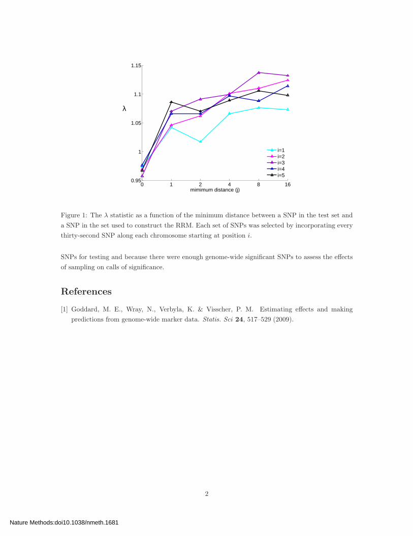
contained approximately 11K SNPs. As shown in Fig. 1, λ generally increased with j for j ≤ 8,

beyond which LD presumably had little effect. Note that the values for λ for the experiments having

the greatest amount of null contamination (j = 0) were quite similar to those when all 367K SNPs

were used to construct the RRM (differences were less than 0.027 over all values of i), suggesting

that our experiment did not deviate substantially from the idealized one.

These experiments show that null-model contamination can be a substantial effect. Consequently,

when using a LMM to test whether a given SNP is associated with the phenotype, the RRM should

be computed from all SNPs except for those in close proximity to the test SNP. As this approach is

again computationally infeasible, in our experiments in the main paper evaluating the accuracy of

association P values, we tested SNPs on chromosome 1 and constructed the “gold-standard” RRM

from all SNPs on all but chromosome 1. We used chromosome 1 because it has a large number of

1


0 1 2 4 8 160.95

1

1.05

1.1

1.15

mimimum distance (j)

λ

i=1i=2i=3i=4i=5

Figure 1: The λ statistic as a function of the minimum distance between a SNP in the test set and

a SNP in the set used to construct the RRM. Each set of SNPs was selected by incorporating every

thirty-second SNP along each chromosome starting at position i.

SNPs for testing and because there were enough genome-wide significant SNPs to assess the effects

of sampling on calls of significance.

References

[1] Goddard, M. E., Wray, N., Verbyla, K. & Visscher, P. M. Estimating effects and making

predictions from genome-wide marker data. Statis. Sci 24, 517–529 (2009).

2


FaST linear mixed models for genome -wide association … we use only one SNP at a time in our work,...

Documents

Transcript of FaST linear mixed models for genome -wide association … we use only one SNP at a time in our work,...