Extended Standard Hough Transform for Analytical Line Recognition
11
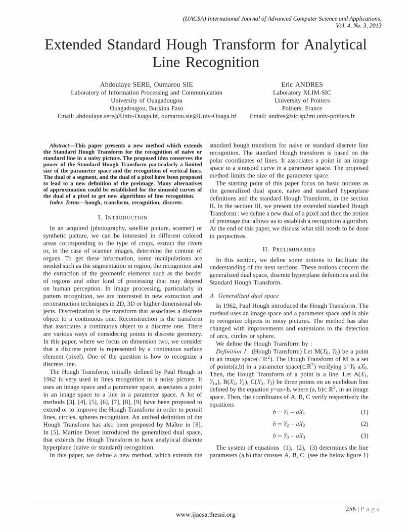
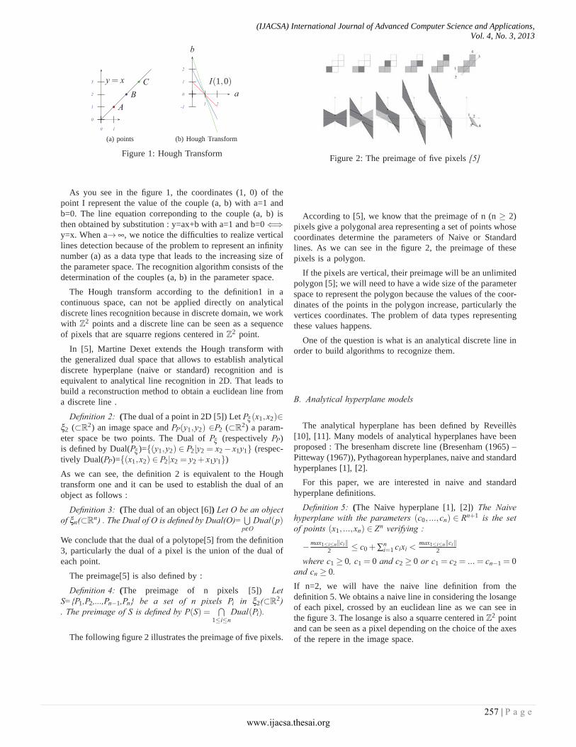
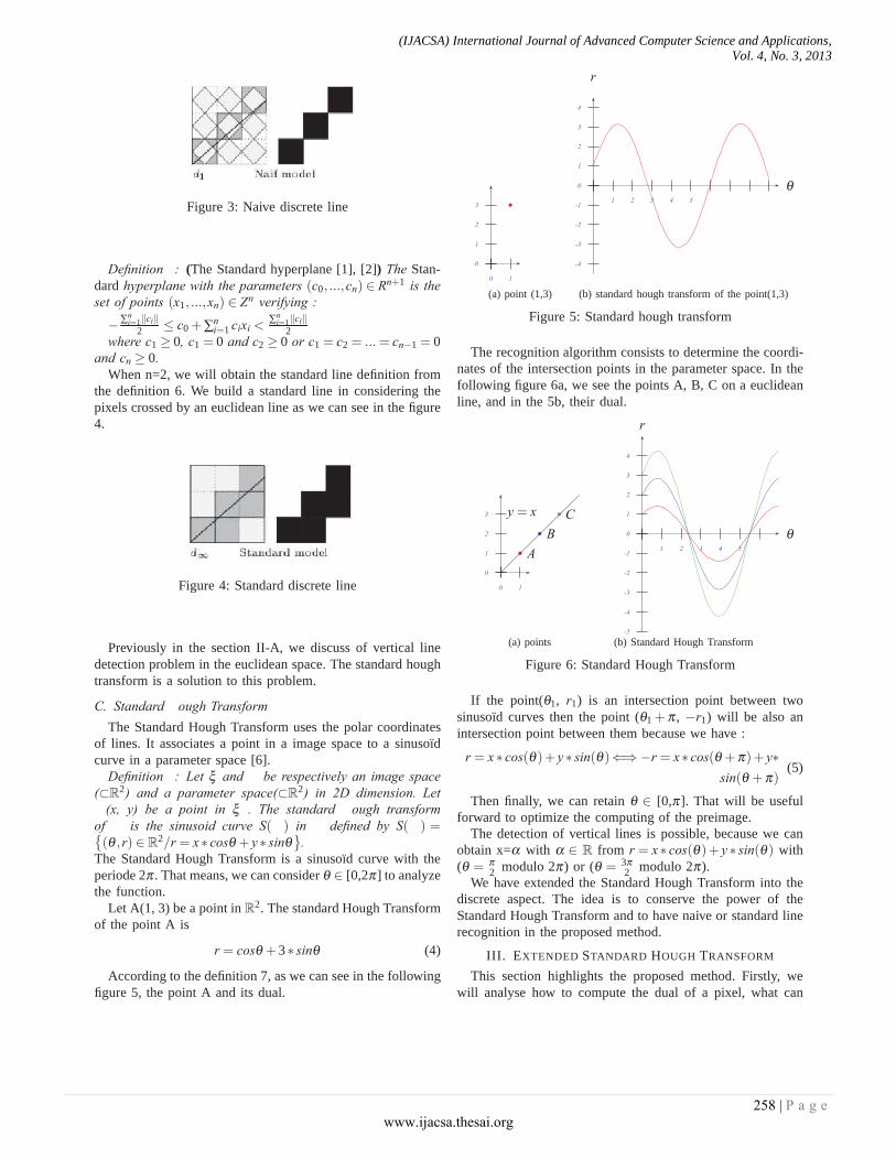
Extended Standard Hough Transform for Analytical Line Recognition Abdoulaye SERE, Oumarou SIE Laboratory of Information Processing and Communication University of Ouagadougou Ouagadougou, Burkina Faso Email: [email protected], [email protected] Eric ANDRES Laboratory XLIM-SIC University of Poitiers Poitiers, France Email: [email protected] Abstract—This paper presents a new method which extends the Standard Hough Transform for the recognition of naive or standard line in a noisy picture. The proposed idea conserves the power of the Standard Hough Transform particularly a limited size of the parameter space and the recognition of vertical lines. The dual of a segment, and the dual of a pixel have been proposed to lead to a new definition of the preimage. Many alternatives of approximation could be established for the sinusoid curves of the dual of a pixel to get new algorithms of line recognition. Index Terms—hough, transform, recognition, discrete. I. I NTRODUCTION In an acquired (photography, satellite picture, scanner) or synthetic picture, we can be interested in different colored areas corresponding to the type of crops, extract the rivers or, in the case of scanner images, determine the contour of organs. To get these information, some manipulations are needed such as the segmentation in region, the recognition and the extraction of the geometric elements such as the border of regions and other kind of processing that may depend on human perception. In image processing, particularly in pattern recognition, we are interested in new extraction and reconstruction techniques in 2D, 3D or higher dimensional ob- jects. Discretization is the transform that associates a discrete object to a continuous one. Reconstruction is the transform that associates a continuous object to a discrete one. There are various ways of considering points in discrete geometry. In this paper, where we focus on dimension two, we consider that a discrete point is represented by a continuous surface element (pixel). One of the question is how to recognize a discrete line. The Hough Transform, initially defined by Paul Hough in 1962 is very used in lines recognition in a noisy picture. It uses an image space and a parameter space, associates a point in an image space to a line in a parameter space. A lot of methods [3], [4], [5], [6], [7], [8], [9] have been proposed to extend or to improve the Hough Transform in order to permit lines, circles, spheres recognition. An unified definition of the Hough Transform has also been proposed by Maître in [8]. In [5], Martine Dexet introduced the generalized dual space, that extends the Hough Transform to have analytical discrete hyperplane (naive or standard) recognition. In this paper, we define a new method, which extends the standard hough transform for naive or standard discrete line recognition. The standard Hough transform is based on the polar coordinates of lines. It associates a point in an image space to a sinusoïd curve in a parameter space. The proposed method limits the size of the parameter space. The starting point of this paper focus on basic notions as the generalized dual space, naive and standard hyperplane definitions and the standard Hough Transform, in the section II. In the section III, we present the extended standard Hough Transform : we define a new dual of a pixel and then the notion of preimage that allows us to establish a recognition algorithm. At the end of this paper, we discuss what still needs to be done in perpectives. II. PRELIMINARIES In this section, we define some notions to facilitate the understanding of the next sections. These notions concern the generalized dual space, discrete hyperplane definitions and the Standard Hough Transform. A. Generalized dual space In 1962, Paul Hough introduced the Hough Transform. The method uses an image space and a parameter space and is able to recognize objects in noisy pictures. The method has also changed with improvements and extensions to the detection of arcs, circles or sphere. We define the Hough Transform by : Definition 1: (Hough Transform) Let M(X 0 , Y 0 ) be a point in an image space(⊂R 2 ). The Hough Transform of M is a set of points(a,b) in a parameter space(⊂R 2 ) verifying b=Y 0 -aX 0 . Then, the Hough Transform of a point is a line. Let A(X 1 , Y 1a ), B(X 2 , Y 2 ), C(X 3 , Y 3 ) be three points on an euclidean line defined by the equation y=ax+b, where (a, b)∈ R 2 , in an image space. Then, the coordinates of A, B, C verify respectively the equations b = Y 1 − aX 1 (1) b = Y 2 − aX 2 (2) b = Y 3 − aX 3 (3) The system of equations (1), (2), (3) determines the line parameters (a,b) that crosses A, B, C. (see the below figure 1) (IJACSA) International Journal of Advanced Computer Science and Applications, Vol. 4, No. 3, 2013 256 | Page www.ijacsa.thesai.org
Transcript of Extended Standard Hough Transform for Analytical Line Recognition
Let A, B, C, D be the vertices of a pixel p as ilustrated inthe figure 9. A pixel is a set of an infinity of vertical segments(9a) or an infinity of horizontal segments (9b). We have alsothe diagonal segments in (9c).
�
C B
AD
(a)
�
C B
AD
(b)
�
C B
AD
(c)
Figure 9: Sides of a pixel
Our aim is to determine the dual of a pixel in going withthe dual of its segments (vertical, diagonal or horizontal).
We propose the following theorem 2.Theorem 2: Let p be a pixel in ξ2(⊂R2) . Its dual is a area
limited by the curve of the duals of its vertical sides. This areais also limited by the curve of the duals of its horizontal sidesor by the duals of its diagonals.
Proof: Let us prove that. Let p be a pixel with its verticesA, B, C, D in image space like in the figure 10.
Firstly, one shows that the dual of a pixel is an area limitedby the dual of its vertical sides [AB] and [CD]. The dual ofa segment is obtained by the theorem 1. Let N be a point ina pixel p with vertices A, B, C, D where N /∈{A, B,C, D}.There exists two points I, J such that N ∈ [IJ] where I ∈[CD],J∈[AB]. We notice that [IJ] is a segment. According to thetheorem 1, the dual of N is a sinusoid curve between the dualsof I and J. As I ∈[CD], J∈[AB], the dual of I is between theduals of the points C and D. The dual of J is also betweenthe duals of the points A and B. So, the dual of N is in thesurfaces limited by the duals of [AB] and [CD]. Inversely, letN’ be a point in the surface limited by the dual of [AB] and[CD]. N’ is between two sinusoïd curves, the duals of twovertices X, Y with (X,Y) ∈{A,B,C,D}2. A pixel is convex,so [XY] ⊂p. According to the theorem 1, there exists a points ∈[XY] in the pixel such as dual(s) is a sinusoïd curve thatpass through N’.
Secondly, one shows that the dual of a pixel is an arealimited by the dual of its horizontal sides [AD] and [BC]. Byanalogy to the first case, we define a point N in a pixel whereN /∈{A, B,C, D}. There exists two points I, J such that N ∈[IJ] where I ∈[AD], J∈[BC]. As I ∈[AD], J∈[BC], the dual ofI is between the duals of A and D. The dual of J is between theduals of B and C. So, the dual of N is in the surfaces limitedby the duals of [AD] and [BC]. We can also notice that whenwe apply on the pixel p, a central symmetry by the center ofthe pixel, a horizontal side become a vertical side. Inversely,let N’ be a point in the surface limited by the dual of [AD]and [BC]. N’ is between two sinusoïd curves, the duals of twovertices X, Y with (X,Y) ∈{A,B,C,D}2. A pixel is convex,so [XY] ⊂p. According to the theorem 1, there exists a point
s ∈[XY] in the pixel such as dual(s) is a sinusoïd curve thatpass through N’.
Thirdly, we show that the dual of a pixel is a surface limitedby the diagonals segments [AC], [BD]. There exists two pointsI, J such that N ∈ [IJ] where I ∈[AC], J∈[BD]. As I ∈[AC],J∈[BD], the dual of I is between the duals of the points Aand C. The dual of J is between the duals of the points B andD. So, the dual of N is in the surfaces limited by the dualsof [AC] and [BD]. Inversely, let N’ be a point in the surfacelimited by the duals of [AC] and [BD]. N’ is between twosinusoïd curves, the duals of two vertices X, Y with (X,Y)∈{A,B,C,D}2. A pixel is convex, so [XY] ⊂p. According tothe theorem 1, there exists a point s ∈[XY] in the pixel suchas dual(s) is a sinusoïd curve which pass through N’.We present an illustration of this proof in the following figure10 where we can see the points N, I, J in the different casesof sides and diagonals : in 10a, we have the vertical sides; in10b, the horizontal sides, and in 10c, the diagonals.
�� �
NI �
C B
AD
(a) [AB] , [CD]
�
�
�
N
I
�C B
AD
(b) [AD], [BC]
�
N� �I �
C B
AD
(c) [AC], [BD]
Figure 10: Segments of pixels
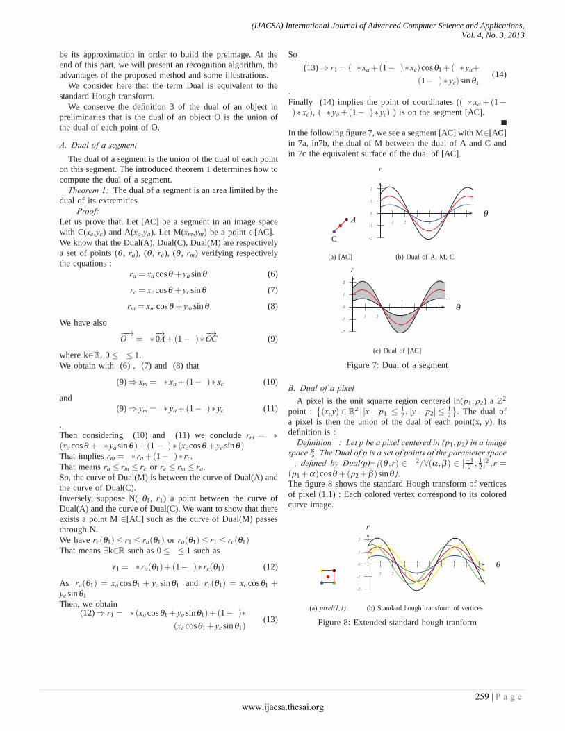
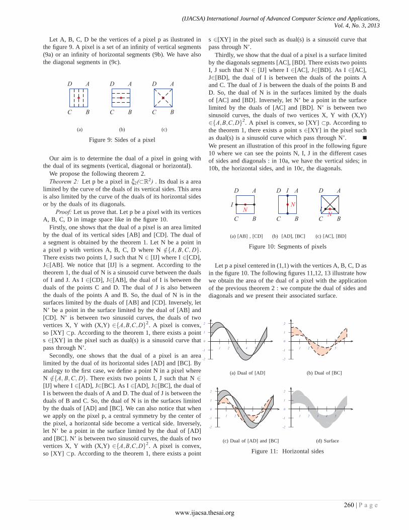
Let p a pixel centered in (1,1) with the vertices A, B, C, D asin the figure 10. The following figures 11,12, 13 illustrate howwe obtain the area of the dual of a pixel with the applicationof the previous theorem 2 : we compute the dual of sides anddiagonals and we present their associated surface.
0
1
2
-1
-2
1 2 3 4 5 �
(a) Dual of [AD]
0
1
2
-1
-2
1 2 3 4 5 �
(b) Dual of [BC]
0
1
2
-1
-2
1 2 3 4 5 �
(c) Dual of [AD] and [BC]
0
1
2
-1
-2
1 2 3 4 5 �
(d) Surface
Figure 11: Horizontal sides
(IJACSA) International Journal of Advanced Computer Science and Applications,
Vol. 4, No. 3, 2013
260 | P a g e www.ijacsa.thesai.org
0
1
2
-1
-2
1 2 3 4 5 �
(a) Dual of [AB]
0
1
2
-1
-2
1 2 3 4 5 �
(b) Dual of [CD]
0
1
2
-1
-2
1 2 3 4 5 �
(c) Dual of [AB] and [CD]
0
1
2
-1
-2
1 2 3 4 5 �
(d) Surface
Figure 12: Vertical sides
0
1
2
-1
-2
1 2 3 4 5 �
(a) Dual of the diagonal [BD]
0
1
2
-1
-2
1 2 3 4 5 �
(b) Dual of the diagonal [AC]
0
1
2
-1
-2
1 2 3 4 5 �
(c) Union of duals
0
1
2
-1
-2
1 2 3 4 5 �
(d) Surface
Figure 13: Diagonals
We observe that in the previous figure 13, there does notexist empty space between the dual of the diagonals. Then, thedual of pixel is easy to be computed by the following theorem3.
Theorem 3: the dual of a pixel is the union of the dual ofits diagonal segments.
Proof: Let us prove that. Let p be a pixel with its verticesA, B, C, D and its diagonals [AC] and [BD]. In the previoustheorem 2, we proved that the dual of a pixel is a surfacebetween the dual of its diagonals. We are going to showthat this area is equivalent to the union of the dual of itsdiagonals. That means, for a point in the dual of a pixel,it must belong to the dual of [AC] or the dual of [BD].[AC] and [BD] are a common point, the center O of the
pixel. So, the dual of O is a sinusoïd curve in the Dual([AC])and the Dual([BD]) according to the theorem1. With θ ∈ [0,2π], we can classify the Dual(A), Dual(B), Dual(O), Dual(C),Dual(D) by the relation≤ or ≥. Dual(O) is in the middle ofthe classification.
Then, we have Dual([AC])⊂ Dual([BD]) or Dual([BD]) ⊂Dual([AC])
As a conclusion, the set of points N verifying the proposition[N∈Dual(p) with N /∈ Dual([AC]) and N /∈ Dual([BD])] is φ .
� ��
�
0
1
2
3
4
0 1 2 3 4
(a) Pixel(1,3)
θ
r
0
1
2
3
4
-1
-2
-3
-4
1 2 3 4 5 � �
(b) Dual of the pixel (1,3)
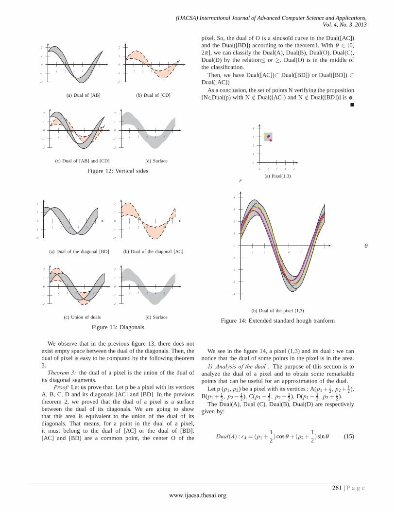
Figure 14: Extended standard hough tranform
We see in the figure 14, a pixel (1,3) and its dual : we cannotice that the dual of some points in the pixel is in the area.
1) Analysis of the dual : The purpose of this section is toanalyze the dual of a pixel and to obtain some remarkablepoints that can be useful for an approximation of the dual.
Let p (p1, p2) be a pixel with its vertices : A(p1+12 , p2+
12 ),
B(p1 +12 , p2− 1
2 ), C(p1− 12 , p2− 1
2 ), D(p1− 12 , p2 +
12 ).
The Dual(A), Dual (C), Dual(B), Dual(D) are respectivelygiven by:
Dual(A) : rA = (p1 +12)cosθ +(p2+
12)sinθ (15)
(IJACSA) International Journal of Advanced Computer Science and Applications,
Vol. 4, No. 3, 2013
261 | P a g e www.ijacsa.thesai.org
Dual(C) : rC = (p1− 12)cosθ +(p2− 1
2)sinθ (16)
Dual(B) : rB = (p1 +12)cosθ +(p2− 1
2)sinθ (17)
Dual(D) : rD = (p1− 12)cosθ +(p2 +
12)sinθ (18)
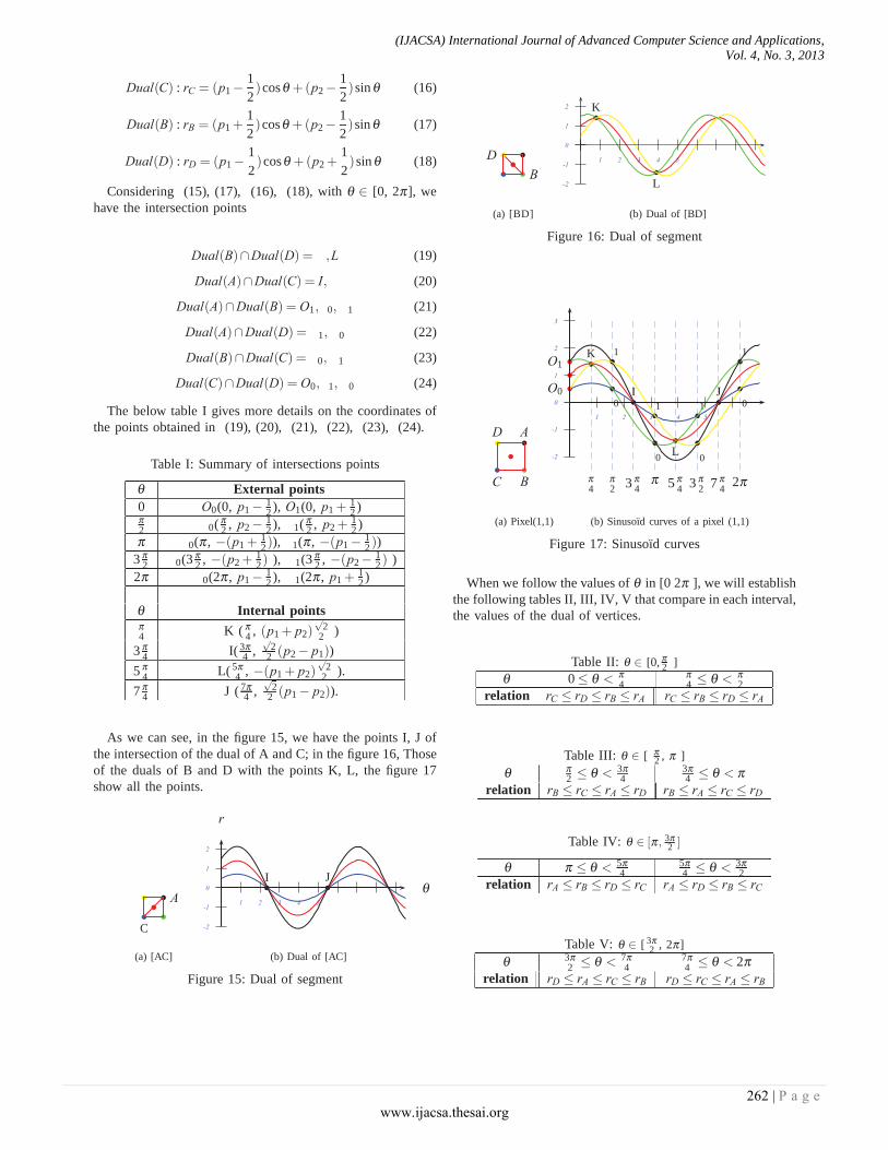
Considering (15), (17), (16), (18), with θ ∈ [0, 2π], wehave the intersection points
Dual(B)∩Dual(D) = �,L (19)
Dual(A)∩Dual(C) = I,� (20)
Dual(A)∩Dual(B) = O1,�0,�1 (21)
Dual(A)∩Dual(D) = �1,�0 (22)
Dual(B)∩Dual(C) = �0,�1 (23)
Dual(C)∩Dual(D) = O0,�1,�0 (24)
The below table I gives more details on the coordinates ofthe points obtained in (19), (20), (21), (22), (23), (24).
Table I: Summary of intersections points
θ External points0 O0(0, p1− 1
2 ), O1(0, p1 +12 )
π2 �0( π
2 , p2− 12 ), �1( π
2 , p2 +12 )
π �0(π , −(p1 +12)), �1(π , −(p1− 1
2 ))3 π
2 �0(3 π2 , −(p2 +
12) ), �1(3 π
2 , −(p2− 12 ) )
2π �0(2π , p1− 12 ), �1(2π , p1 +
12 )
θ Internal pointsπ4 K ( π
4 , (p1 + p2)√
22 )
3 π4 I( 3π
4 ,√
22 (p2− p1))
5 π4 L( 5π
4 , −(p1 + p2)√
22 ).
7 π4 J ( 7π
4 ,√
22 (p1− p2)).
As we can see, in the figure 15, we have the points I, J ofthe intersection of the dual of A and C; in the figure 16, Thoseof the duals of B and D with the points K, L, the figure 17show all the points.
�
� �
C
� A�
(a) [AC]
θ
r
�
I�
J0
1
2
-1
-2
1 2 3 4 5 � � � �
(b) Dual of [AC]
Figure 15: Dual of segment
�
� �
D �
B
�
(a) [BD]
�
K
�
L
0
1
2
-1
-2
1 2 3 4 5 � � � �
(b) Dual of [BD]
Figure 16: Dual of segment
�
� �
��
C B
AD
(a) Pixel(1,1)
O1
O0 �
�0
�
�1
�
�0
�
�1
�
�0
�
�1
�
�0
�
�1�
�
�
�
K
�
L
�
I�
J
π4
π2 3 π
4π 5 π
4 3 π2 7 π
4 2π
0
1
2
3
-1
-2
1 2 3 4 5 �
(b) Sinusoïd curves of a pixel (1,1)
Figure 17: Sinusoïd curves
When we follow the values of θ in [0 2π ], we will establishthe following tables II, III, IV, V that compare in each interval,the values of the dual of vertices.
Table II: θ ∈ [0, π2 ]
θ 0≤ θ < π4
π4 ≤ θ < π
2relation rC ≤ rD ≤ rB ≤ rA rC ≤ rB ≤ rD ≤ rA
Table III: θ ∈ [ π2 , π ]
θ π2 ≤ θ < 3π
43π4 ≤ θ < π
relation rB ≤ rC ≤ rA ≤ rD rB ≤ rA ≤ rC ≤ rD
Table IV: θ ∈ [π, 3π2 ]
θ π ≤ θ < 5π4
5π4 ≤ θ < 3π
2relation rA ≤ rB ≤ rD ≤ rC rA ≤ rD ≤ rB ≤ rC
Table V: θ ∈ [ 3π2 , 2π]
θ 3π2 ≤ θ < 7π
47π4 ≤ θ < 2π
relation rD ≤ rA ≤ rC ≤ rB rD ≤ rC ≤ rA ≤ rB
(IJACSA) International Journal of Advanced Computer Science and Applications,
Vol. 4, No. 3, 2013
262 | P a g e www.ijacsa.thesai.org
When θ passes the values π2 , π , 3 π
2 , 2π , we will observethat the exteriors ri become the interiors ri′ and inversely.
According to
r = x∗ cosθ + y∗ sinθ ⇐⇒−r = x∗ cos(θ +π)+ y∗sin(θ +π)
(25)
we will work on an interval [0, π], with the tables II, IIIand the external or internal points of this interval. The othersexterior or interior points and the tables IV, V are deductions.
2) Approximation of the dual : Here, we propose an ap-proximation of the area of the dual of a pixel. In computationalgeometry, algorithms exists to compute the intersection of con-vex polygons. A lot of methods of approximation possibilitycould be studied forward.
In our method, we consider a polygonal approximationbased on a few points of the dual in the way to obtain someparameters (θ , r) : the idea is that if an object O’ is anapproximation of an object O then Dual(O’) will be also anapproximation of Dual(O).
Moreover, if O’⊂O, we will have Dual(O’)⊂Dual(O). Somepoints of the initial pixel are used to obtain its dual approxi-mation.Let p be a pixel centered in (p1,p2). The pixel p has thevertices A(p1 +
12 , p2 +
12 ), B(p1 +
12 , p2 − 1
2 ), C(p1 − 12 ,
p2− 12 ), D(p1− 1
2 , p2 +12 ).
Let pi be a pixel centered in (p1,p2) with its vertices Ai(p1+12 − i∗ δ , p2 +
12 ), Bi(p1 +
12 , p2− 1
2 + i∗ δ ), Ci(p1− 12 + i∗ δ ,
p2− 12 ), Di(p1− 1
2 , p2 +12 − i∗ δ ).
where i∈ N and δ∈[0,1] with the contraints i∗δ∈{0,1]. Theduals of the vertices of pi are :
Dual(Ai) : rAi = (p1 +12− i∗ δ )cosθ +(p2+
12)sinθ (26)
Dual(Ci) : rCi = (p1− 12+ i∗ δ )cosθ +(p2− 1
2)sinθ (27)
Dual(Bi) : rBi = (p1 +12)cosθ +(p2− 1
2+ i∗ δ )sinθ (28)
Dual(Di) : rDi = (p1− 12)cosθ +(p2+
12− i∗ δ )sinθ (29)
Then, pi is an approximative pixel of p where i ∗ δ is thedifference with the real vertice coordinates of p. The maximalvalue of i∗δ must be inferior to the maximal of the toleranceerror.
We use the external points (see the table I) of the dual ofthe pixels p0, p1, p2,... pn to get a polygonal approximationof the dual of p with p0 = pn+1 = p.We know that
pn+1 = p⇐⇒ (n+1)∗ δ = 1 (30)
Then (30)⇐⇒ δ = 1n+1 .
Finally, we need to take δ = 1n+1 to have the pixels p0, p1,
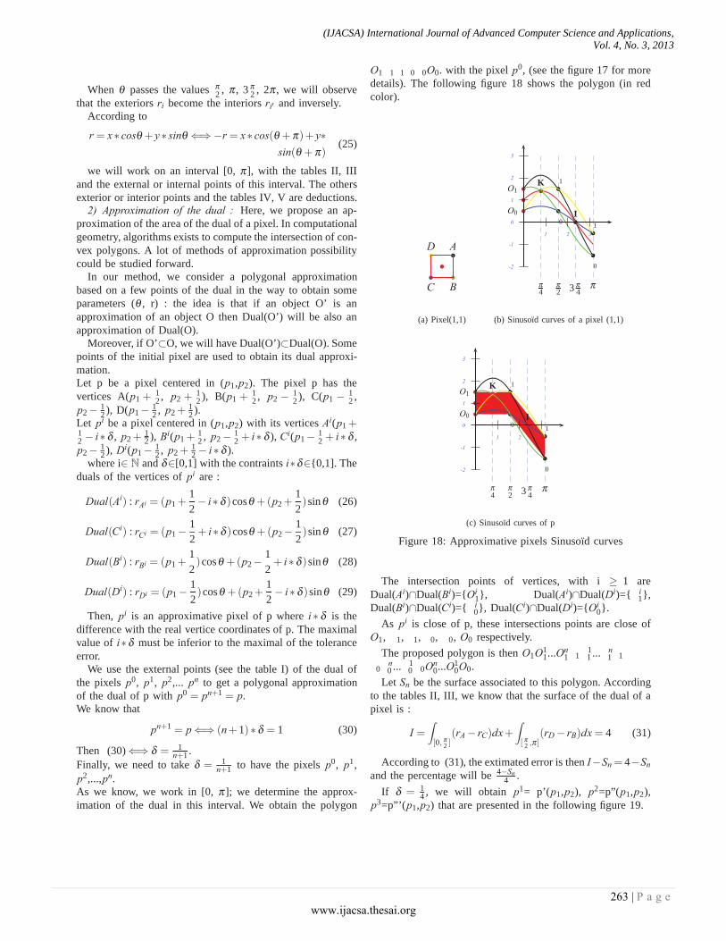
p2,...,pn.As we know, we work in [0, π]; we determine the approx-imation of the dual in this interval. We obtain the polygon
O1�1�1�0�0O0. with the pixel p0, (see the figure 17 for moredetails). The following figure 18 shows the polygon (in redcolor).
�
� �
��
C B
AD
(a) Pixel(1,1)
O1
O0 �
�0
�
�1
�
�0
�
�1
�
�
�
�
K
�
I
π4
π2 3 π
4π
0
1
2
3
-1
-2
1 2 3
(b) Sinusoïd curves of a pixel (1,1)
O1
O0 �
�0
�
�1
�
�0
�
�1
�
�
�
�
K
�
π4
π2 3 π
4π
I0
1
2
3
-1
-2
1 2 3
(c) Sinusoïd curves of p
Figure 18: Approximative pixels Sinusoïd curves
The intersection points of vertices, with i ≥ 1 areDual(Ai)∩Dual(Bi)={Oi
1}, Dual(Ai)∩Dual(Di)={�i1},
Dual(Bi)∩Dual(Ci)={�i0}, Dual(Ci)∩Dual(Di)={Oi
0}.As pi is close of p, these intersections points are close of
O1, �1, �1, �0, �0, O0 respectively.The proposed polygon is then O1O1
1...On1�1�1
1 ...�n1�1
�0�n0 ...�1
0�0On0...O1
0O0.Let Sn be the surface associated to this polygon. According
to the tables II, III, we know that the surface of the dual of apixel is :
I =∫[0, π
2 ](rA− rC)dx+
∫[ π
2 ,π ](rD− rB)dx = 4 (31)
According to (31), the extimated error is then I−Sn = 4−Snand the percentage will be 4−Sn
4 .If δ = 1
4 , we will obtain p1= p’(p1,p2), p2=p”(p1,p2),p3=p”’(p1,p2) that are presented in the following figure 19.
(IJACSA) International Journal of Advanced Computer Science and Applications,
Vol. 4, No. 3, 2013
263 | P a g e www.ijacsa.thesai.org
� �
��
C′B′
A′
D′ �
�
�
�
�
(a) pixel p’
� �
��
D′′
C′′
B′′
A′′
�
�
�
�
�
(b) pixel p”
�
� �
��
D′′′
C′′′
B′′′A′′′
�
�
�
�
�
(c) pixel p”’
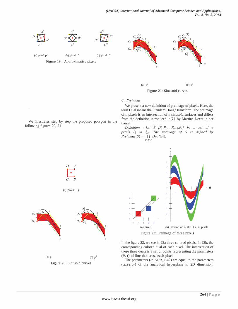
Figure 19: Approximative pixels
.
We illustrates step by step the proposed polygon in thefollowing figures 20, 21
�
� �
��
C B
AD
(a) Pixel(1,1)
O1
O0 �
�0
�
�1
�
�0
�
�1
�
�
�
�
K
�
I
(b) p
O1
O0 �
�0
�
�1
�
�0
�
�1
�
�
�
�
O11
�
O10 �
�10
�
�11
K
�
I
(c) p1
Figure 20: Sinusoïd curves
O1
O0 �
�0
�
�1
�
�0
�
�1
�
�
�
O11
�
O10 �
�10
�
O21
�
O20
��2
1
�
�20
�
�11
(a) p2
O1
O0 �
�0
�
�1
� �0
� �1
�
�
�
O11
�
O10 �
�10
�
O21
�
O20
��2
1
�
�20
�
O31
�
O30
�
�31
�
�30
�
�11
(b) p3
Figure 21: Sinusoïd curves
C. PreimageWe present a new definition of preimage of pixels. Here, the
term Dual means the Standard Hough transform. The preimageof n pixels is an intersection of n sinusoïd surfaces and differsfrom the definition introduced in[?], by Martine Dexet in herthesis.
Definition �: Let S={P1,P2,...,Pn−1,Pn} be a set of npixels Pi in ξ2. The preimage of S is defined byPreimage(S) =
⋂1≤i≤n
Dual(Pi).
0
1
2
3
4
0 1 2 3 4
(a) pixels
θ
r
0
1
2
3
4
5
�
-1
-2
-3
-4
-5
-�
1 2 3 4 5 �
(b) Intersection of the Dual of pixels
Figure 22: Preimage of three pixels
In the figure 22, we see in 22a three colored pixels. In 22b, thecorresponding colored dual of each pixel. The intersection ofthese three duals is a set of points representing the parameters(θ , r) of line that cross each pixel.
The parameters (-r, cosθ , sinθ ) are equal to the parameters(c0,c1,c2) of the analytical hyperplane in 2D dimension,
(IJACSA) International Journal of Advanced Computer Science and Applications,
Vol. 4, No. 3, 2013
264 | P a g e www.ijacsa.thesai.org
presented in the section II-B. As you can see in the figure22 the preimage of n pixels give two areas because
r = x∗ cosθ + y∗ sinθ ⇐⇒−r = x∗ cos(θ +π)+ y∗sin(θ +π)
(32)
D. Recognition algorithmIn this part, we recall that the term dual indicates the
Extended Standard Hough Transform. We can see that when,the dual of the losange of each pixel is considered, we willbe in the case of naive line recognition.
Moreover, according to the definition of the naive andstandard hyperplanes introduced in preliminaries and the ge-ometry construction of these models, we see that the preimagecontains the parameters of analytical line that crosses thepixels.
We propose the following algorithm :
Algorithm 1 Naive, Standard line recognitionData : A set S of n pixels P1,..., Pn.Begin
Preimage←Dual(P1)i←2while Preimage �= Ø and i≤ n do
Preimage←Preimage ∩ Dual(Pi)i←i+1
End whileif Preimage �= Ø then
S belongs to a digital lineelse
S does not belong to a digital lineEnd if
End
The Dual(Pi) could be replaced by an approximation (poly-gon for example) in order to increase the performance of thealgorithm.
The Extended Standard Hough Transform has its particu-larity to answer the question how can we recognize Naiveand Standard by the standard Hough Transform. It conservesthe properties of the Standard Hough Transform [6] as thesize of the parameter space is limited [6]:θ ∈ [0, π] and r∈[0,
√col2 + row2} with an image col x row. This leads to the
vertical line detection.
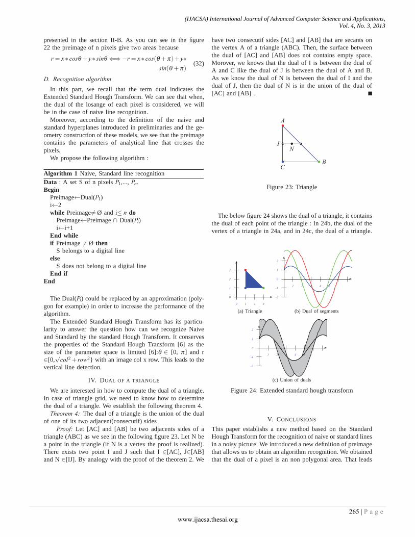
IV. DUAL OF A TRIANGLE
We are interested in how to compute the dual of a triangle.In case of triangle grid, we need to know how to determinethe dual of a triangle. We establish the following theorem 4.
Theorem 4: The dual of a triangle is the union of the dualof one of its two adjacent(consecutif) sides
Proof: Let [AC] and [AB] be two adjacents sides of atriangle (ABC) as we see in the following figure 23. Let N bea point in the triangle (if N is a vertex the proof is realized).There exists two point I and J such that I ∈[AC], J∈[AB]and N ∈[IJ]. By analogy with the proof of the theorem 2. We
have two consecutif sides [AC] and [AB] that are secants onthe vertex A of a triangle (ABC). Then, the surface betweenthe dual of [AC] and [AB] does not contains empty space.Morover, we knows that the dual of I is between the dual ofA and C like the dual of J is between the dual of A and B.As we know the dual of N is between the dual of I and thedual of J, then the dual of N is in the union of the dual of[AC] and [AB] .
� ��I �
N
�
A
� B�
C
Figure 23: Triangle
The below figure 24 shows the dual of a triangle, it containsthe dual of each point of the triangle : In 24b, the dual of thevertex of a triangle in 24a, and in 24c, the dual of a triangle.
�
��
0
1
2
3
0 1 2 3
(a) Triangle
0
1
2
-1
-2
1 2 3 4 5 � �
(b) Dual of segments
0
1
2
-1
-2
1 2 3 4 5 � �
(c) Union of duals
Figure 24: Extended standard hough transform
V. CONCLUSIONS
This paper establishs a new method based on the StandardHough Transform for the recognition of naive or standard linesin a noisy picture. We introduced a new definition of preimagethat allows us to obtain an algorithm recognition. We obtainedthat the dual of a pixel is an non polygonal area. That leads
(IJACSA) International Journal of Advanced Computer Science and Applications,
Vol. 4, No. 3, 2013
265 | P a g e www.ijacsa.thesai.org
to propose an approximation. Others approximative methodscould be studied deeply forward in the objectif to improve thealgorithm. Some works still left to be done, particularly theimplemention on concrete pictures. The dual of a triangle hasbeen proposed. That could give interested perpectives in theothers grids. One of the remaining question is to extend themethod in 3D.
ACKNOWLEGDMENT
The authors would like to thank the organization “L’AgenceUniversitaire de la Francophonie”(AUF) for their help andsupport in making this work possible.
REFERENCES
[1] E. Andres. Discrete linear objects in dimension n : the standardmodel. Graphical Models, pages 65 :92–111, 2003.
[2] E. Andres, R. Acharya, C. Sibata, Discrete analytical hyper-planes, Graphical Model and Image processing, Volume 59,Issue 5, September 1997, Pages 302–309.
[3] D.H.Ballard. Generalizing the hough transform to detect arbi-trary shapes. Pattern Recognition, Vol. 13, No. 2, pp. 111–112,1981.
[4] M Bruckstein, N.Kiryati, Y.Eldar. A probabilistic hough trans-form. Pattern Recognition, 24(4) : 303–316, 1991.
[5] M.Dexet. Architecture d’un modéleur géometrique à basetopologique d’objets discrets et methodes de reconstruction endimensions 2 et 3. Thèse de Doctorat, Université de Poitiers,France, 2006.
[6] F. Dubeau, S.El mejdani, R.Egli. Champs de hauteur de latransformée de hough standard. Actes de 4ième Conférence In-ternationale en Recherche Opérationnelle, pages 133-144, 2005.
[7] J. Cha , R. H. Cofer , S. P. Kozaitis, Extended Hough trans-form for linear feature detection, Pattern Recognition, v.39 n.6,p.1034-1043, June, 2006
[8] H.Maître. Un panorama de la transformée de hough - a reviewon hough transform. Traitement du Signal, 2(4) :305–317, 1985.
[9] J. Matas, C. Galambosy and J. Kittler. Progressive probabilistichough transform, Transform, Volume: 24, n.4, Pages: 303-316,1991
[10] J. P Reveillès, combinatorial pieces in digital lines and planes,in Vision Geometry IV Proc. SPIE, Vol. 2573, San Diego, CA,1995, pp. 23-24.
[11] J.P. Reveillès. Géométrie discrète, Calcul en nombres entierset algorithmiques. Thèse d’état, Université Louis Pasteur, Stras-bourg, France, 1991
(IJACSA) International Journal of Advanced Computer Science and Applications,
Vol. 4, No. 3, 2013
266 | P a g e www.ijacsa.thesai.org