BANOCOSS, Norrfallsviken, Sweden, June 13-17, 2011

Extended Sampford sampling,

balanced Pareto sampling,

and sampling with prescribed

second-order inclusion probabilities

Lennart Bondesson

Dept of Math. & Math. Statistics, Umea University,SE-90187 Umea, Sweden

0. Introduction

Population U = {1,2, . . . , N}.

How to sample n units with prescribed inclusion probabilities

πi, i = 1,2, . . . , N, with sum n is a topic with a long history (e.g.

Brewer & Hanif 1983, Chaudhuri & Vos 1988, Tille 2006).

Many researchers have contributed to the theory of πps sam-

pling. There are many solutions. Different samplers have differ-

ent favourite solutions.

Many samplers just press a button, but maybe not the best one.

I look upon a sample as binary N-vector x. Thus a sample of

size n = 3 from a population of size N = 20 is described as

x = [0,0,1,0,0,0,0,0,0,0,0,1,0,1,0,0,0,0,0,0]

and not as s = {3,12,14}. The first notation simplifies a lot! A

design is described by its probability function p(x) = Pr(I = x).

Three important πps sampling designs:

• The conditional Poisson (CP) design

• The Sampford design

• The Pareto design

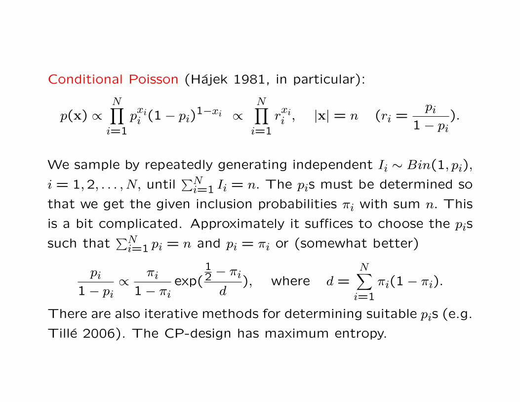
Conditional Poisson (Hajek 1981, in particular):

p(x) ∝N∏

i=1

pxii (1− pi)

1−xi ∝N∏

i=1

rxii , |x| = n (ri =

pi

1− pi).

We sample by repeatedly generating independent Ii ∼ Bin(1, pi),

i = 1,2, . . . , N, until∑N

i=1 Ii = n. The pis must be determined so

that we get the given inclusion probabilities πi with sum n. This

is a bit complicated. Approximately it suffices to choose the pis

such that∑N

i=1 pi = n and pi = πi or (somewhat better)

pi

1− pi∝

πi

1− πiexp(

12 − πi

d), where d =

N∑i=1

πi(1− πi).

There are also iterative methods for determining suitable pis (e.g.

Tille 2006). The CP-design has maximum entropy.

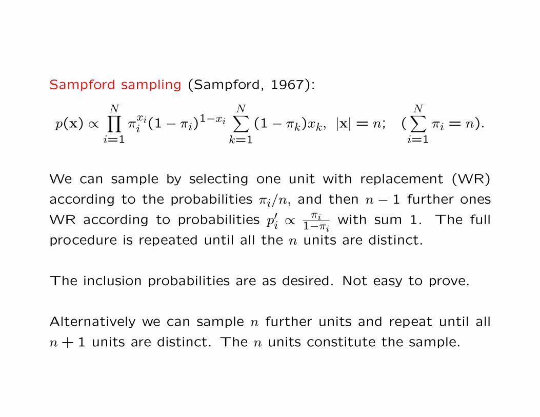
Sampford sampling (Sampford, 1967):

p(x) ∝N∏

i=1

πxii (1− πi)

1−xi

N∑k=1

(1− πk)xk, |x| = n; (N∑

i=1

πi = n).

We can sample by selecting one unit with replacement (WR)

according to the probabilities πi/n, and then n − 1 further ones

WR according to probabilities p′i ∝πi

1−πiwith sum 1. The full

procedure is repeated until all the n units are distinct.

The inclusion probabilities are as desired. Not easy to prove.

Alternatively we can sample n further units and repeat until all

n + 1 units are distinct. The n units constitute the sample.

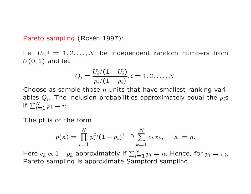
Pareto sampling (Rosen 1997):

Let Ui, i = 1,2, . . . , N, be independent random numbers fromU(0,1) and let

Qi =Ui/(1− Ui)

pi/(1− pi), i = 1,2, . . . , N.

Choose as sample those n units that have smallest ranking vari-ables Qi. The inclusion probabilities approximately equal the pisif∑N

i=1 pi = n.

The pf is of the form

p(x) =N∏

i=1

pxii (1− pi)

1−xi

N∑k=1

ckxk, |x| = n.

Here ck ∝ 1− pk approximately if∑N

i=1 pi = n. Hence, for pi = πi,

Pareto sampling is approximate Sampford sampling.

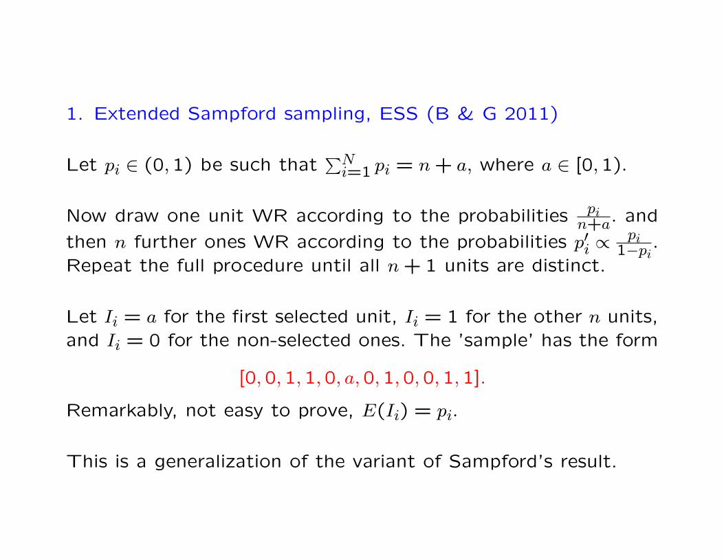
1. Extended Sampford sampling, ESS (B & G 2011)

Let pi ∈ (0,1) be such that∑N

i=1 pi = n + a, where a ∈ [0,1).

Now draw one unit WR according to the probabilities pin+a. and

then n further ones WR according to the probabilities p′i ∝pi

1−pi.

Repeat the full procedure until all n + 1 units are distinct.

Let Ii = a for the first selected unit, Ii = 1 for the other n units,and Ii = 0 for the non-selected ones. The ’sample’ has the form

[0,0,1,1,0, a,0,1,0,0,1,1].

Remarkably, not easy to prove, E(Ii) = pi.

This is a generalization of the variant of Sampford’s result.

Some other πps sampling methods also easily permit this type ofextension, for example systematic πps sampling, pivotal sampling(Deville & Tille 1998), and Pareto sampling.

For Pareto sampling, we let the unit corresponding to the orderstatistic Q(n+1) get Ii = a.

From [0,0,1,1,0, a,0,1,0,0,1,1], we can get a sample of tra-ditional form by making an additional random experiment withchance a to succeed. The sample size is then random, n or n+1.

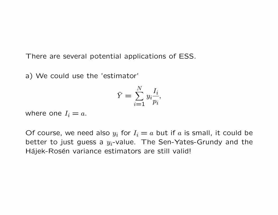
There are several potential applications of ESS.

a) We could use the ’estimator’

Y =N∑

i=1

yiIi

pi,

where one Ii = a.

Of course, we need also yi for Ii = a but if a is small, it could bebetter to just guess a yi-value. The Sen-Yates-Grundy and theHajek-Rosen variance estimators are still valid!

b) Sampford sampling with prescribed πis with sum n is oftentime consuming and it may happen that no sample is provided.

However, we can select M units by SRSWOR from {1,2, . . . , N}and then pick an extended Sampford sample among these M

units of the type [0,1,1, a,0,1,1,0]. Thus for all the M units,except one, the outcome (0 or 1) is decided. There remainN −M +1 units for which the sampling outcome is not decided.We just repeat on these units the procedure. It is repeated untilthe outcome 0 or 1 is obtained for all units.

For M = 2 this method agrees with Deville & Tille’s (1998)pivotal method for which the entropy is not so high. For M > 2(not too small), the sample probabilities are very close to thoseof ordinary Sampford sampling. The samples are obtained veryrapidly if M is not too large.

c) Sampling in blocks (real time sampling)

Units may come in blocks to the sampler (or the sampler mayvisit blocks of units). The inclusion probabilities may be propor-tional to some auxiliary variable and are determined in advance(common in forestry, for instance). These inclusion probabilitiesneed not sum to integers for units in a block.

We may then use for each block ESS. For each block there re-main exactly one unit for which the outcome is not yet decided.Then we may use just systematic πps sampling on these remain-ing units. Then the outcome can be decided immediately for allunits in a block.

d) ESS can also be used to perform stratified sampling πps sam-pling with several stratifications.

For the cross-strata the inclusion probabilities need not sum tointegers. Deville & Tille’s (2004) cube method may replace thesystematic πps sampling in (c). We get high entropy.

More details in B & G (2011).

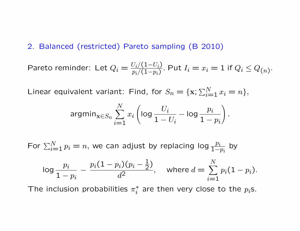
2. Balanced (restricted) Pareto sampling (B 2010)

Pareto reminder: Let Qi = Ui/(1−Ui)pi/(1−pi)

. Put Ii = xi = 1 if Qi ≤ Q(n).

Linear equivalent variant: Find, for Sn = {x;∑N

i=1 xi = n},

argminx∈Sn

N∑i=1

xi

(log

Ui

1− Ui− log

pi

1− pi

).

For∑N

i=1 pi = n, we can adjust by replacing log pi1−pi

by

logpi

1− pi−

pi(1− pi)(pi − 12)

d2, where d =

N∑i=1

pi(1− pi).

The inclusion probabilities π∗i are then very close to the pis.

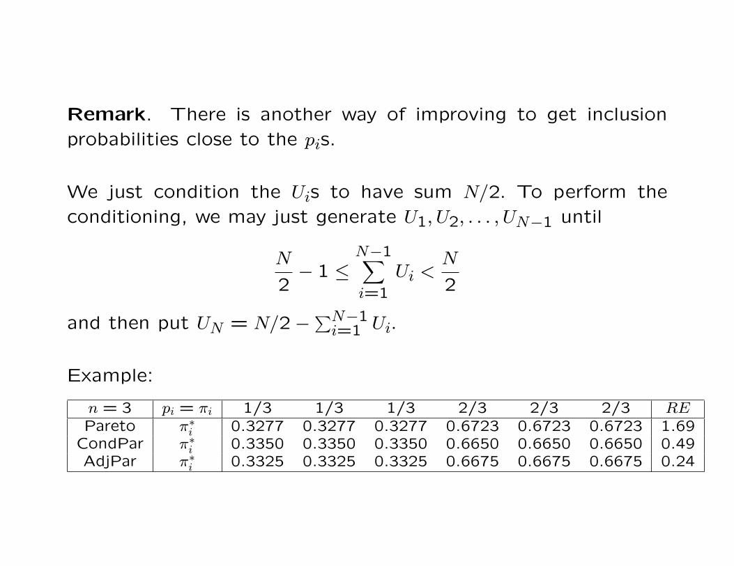
Remark. There is another way of improving to get inclusion

probabilities close to the pis.

We just condition the Uis to have sum N/2. To perform the

conditioning, we may just generate U1, U2, . . . , UN−1 until

N

2− 1 ≤

N−1∑i=1

Ui <N

2

and then put UN = N/2−∑N−1

i=1 Ui.

Example:

n = 3 pi = πi 1/3 1/3 1/3 2/3 2/3 2/3 REPareto π∗i 0.3277 0.3277 0.3277 0.6723 0.6723 0.6723 1.69

CondPar π∗i 0.3350 0.3350 0.3350 0.6650 0.6650 0.6650 0.49AdjPar π∗i 0.3325 0.3325 0.3325 0.6675 0.6675 0.6675 0.24

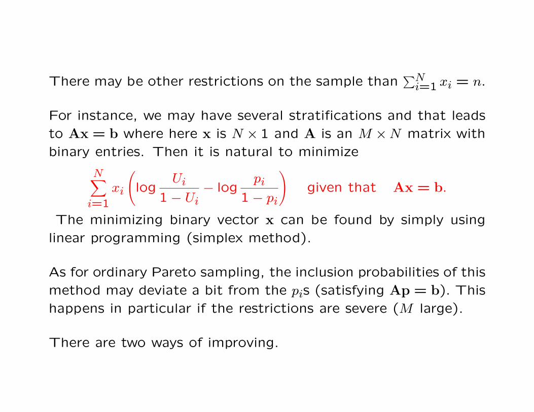
There may be other restrictions on the sample than∑N

i=1 xi = n.

For instance, we may have several stratifications and that leads

to Ax = b where here x is N × 1 and A is an M ×N matrix with

binary entries. Then it is natural to minimize

N∑i=1

xi

(log

Ui

1− Ui− log

pi

1− pi

)given that Ax = b.

The minimizing binary vector x can be found by simply using

linear programming (simplex method).

As for ordinary Pareto sampling, the inclusion probabilities of this

method may deviate a bit from the pis (satisfying Ap = b). This

happens in particular if the restrictions are severe (M large).

There are two ways of improving.

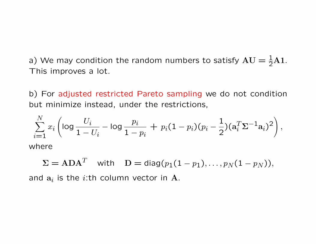
a) We may condition the random numbers to satisfy AU = 12A1.

This improves a lot.

b) For adjusted restricted Pareto sampling we do not condition

but minimize instead, under the restrictions,

N∑i=1

xi

(log

Ui

1− Ui− log

pi

1− pi+ pi(1− pi)(pi −

1

2)(aT

i Σ−1ai)2)

,

where

Σ = ADAT with D = diag(p1(1− p1), . . . , pN(1− pN)),

and ai is the i:th column vector in A.

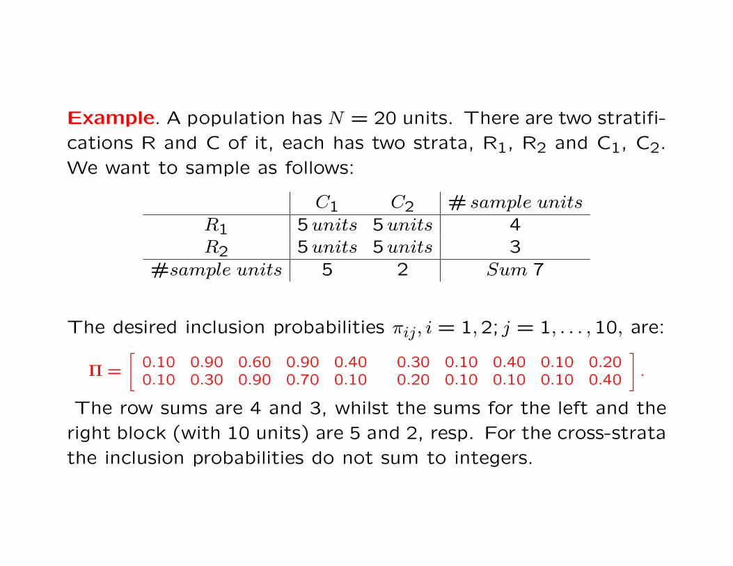
Example. A population has N = 20 units. There are two stratifi-

cations R and C of it, each has two strata, R1, R2 and C1, C2.

We want to sample as follows:

C1 C2 # sample unitsR1 5units 5units 4R2 5units 5units 3

#sample units 5 2 Sum 7

The desired inclusion probabilities πij, i = 1,2; j = 1, . . . ,10, are:

Π =

[0.10 0.90 0.60 0.90 0.40 0.30 0.10 0.40 0.10 0.200.10 0.30 0.90 0.70 0.10 0.20 0.10 0.10 0.10 0.40

].

The row sums are 4 and 3, whilst the sums for the left and the

right block (with 10 units) are 5 and 2, resp. For the cross-strata

the inclusion probabilities do not sum to integers.

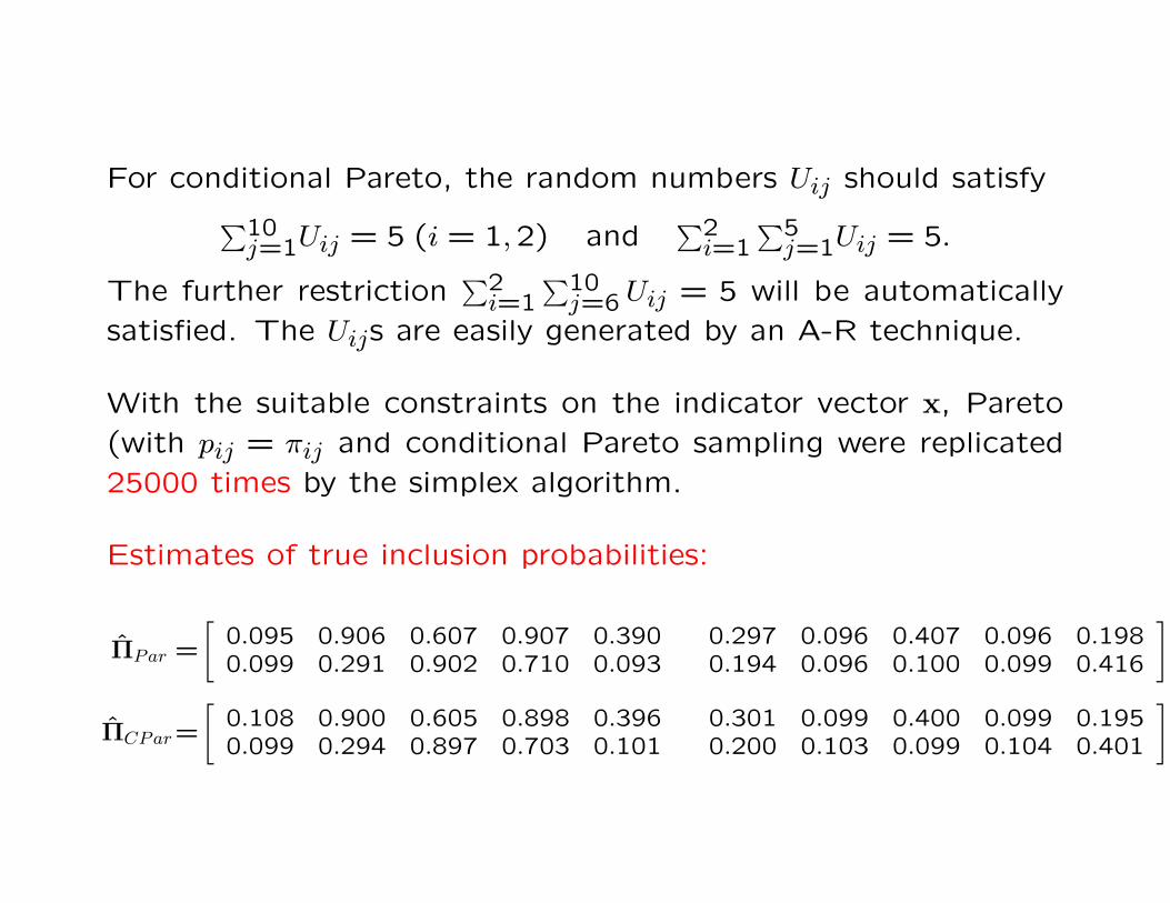
For conditional Pareto, the random numbers Uij should satisfy∑10j=1Uij = 5 (i = 1,2) and

∑2i=1

∑5j=1Uij = 5.

The further restriction∑2

i=1∑10

j=6 Uij = 5 will be automatically

satisfied. The Uijs are easily generated by an A-R technique.

With the suitable constraints on the indicator vector x, Pareto

(with pij = πij and conditional Pareto sampling were replicated

25000 times by the simplex algorithm.

Estimates of true inclusion probabilities:

ΠPar =

[0.095 0.906 0.607 0.907 0.390 0.297 0.096 0.407 0.096 0.1980.099 0.291 0.902 0.710 0.093 0.194 0.096 0.100 0.099 0.416

]ΠCPar=

[0.108 0.900 0.605 0.898 0.396 0.301 0.099 0.400 0.099 0.1950.099 0.294 0.897 0.703 0.101 0.200 0.103 0.099 0.104 0.401

].

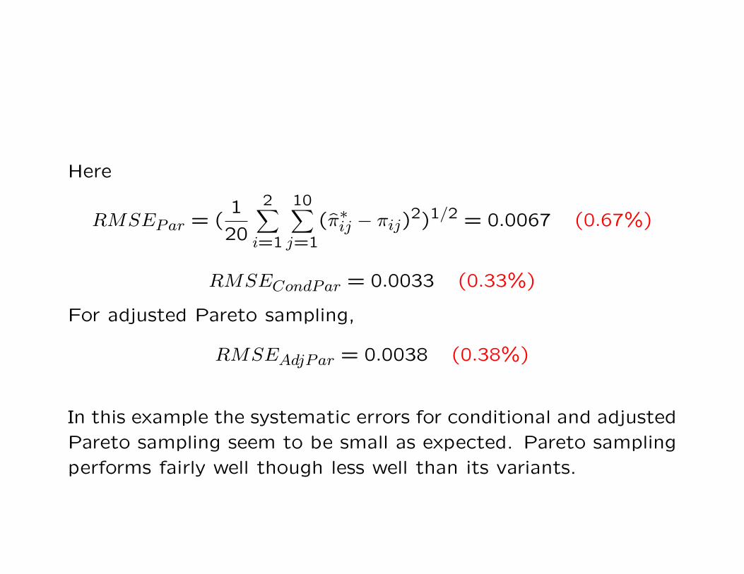
Here

RMSEPar = (1

20

2∑i=1

10∑j=1

(π∗ij − πij)2)1/2 = 0.0067 (0.67%)

RMSECondPar = 0.0033 (0.33%)

For adjusted Pareto sampling,

RMSEAdjPar = 0.0038 (0.38%)

In this example the systematic errors for conditional and adjusted

Pareto sampling seem to be small as expected. Pareto sampling

performs fairly well though less well than its variants.

Pareto sampling in all variants has a big advantage compared

with other methods:

We can use the random numbers Ui as permanent random num-

bers and thereby improve estimates of changes. This is often

referred to as sample coordination.

3. Sampling with prescribed 2nd order inclusion probabilities πij

Old problem going back to Hanurav (1966). For instance, two

units that are likely to have similar y-values should have a low

joint inclusion probability. Simple solution by Sinha (1973) but

it works only for designs very close to SRSWOR.

We consider inclusion probability matrices, IPMs, (πij) of designs

of fixed size n. These IPMs constitute a very complicated convex

polyhedron. However, there is a fairly simple characterization:

Theorem. Let 2 ≤ n ≤ N − 2. A symmetric matrix (πij) is an

IPM for a design of size n if and only if πij =∑

x; |x|=n xixjp(x),

where p(x) ∝ exp(∑{i,j} aijxixj) (sum over pairs {i, j}, i 6= j) and

aij = aji ∈ R, or a limit of such IPMs.

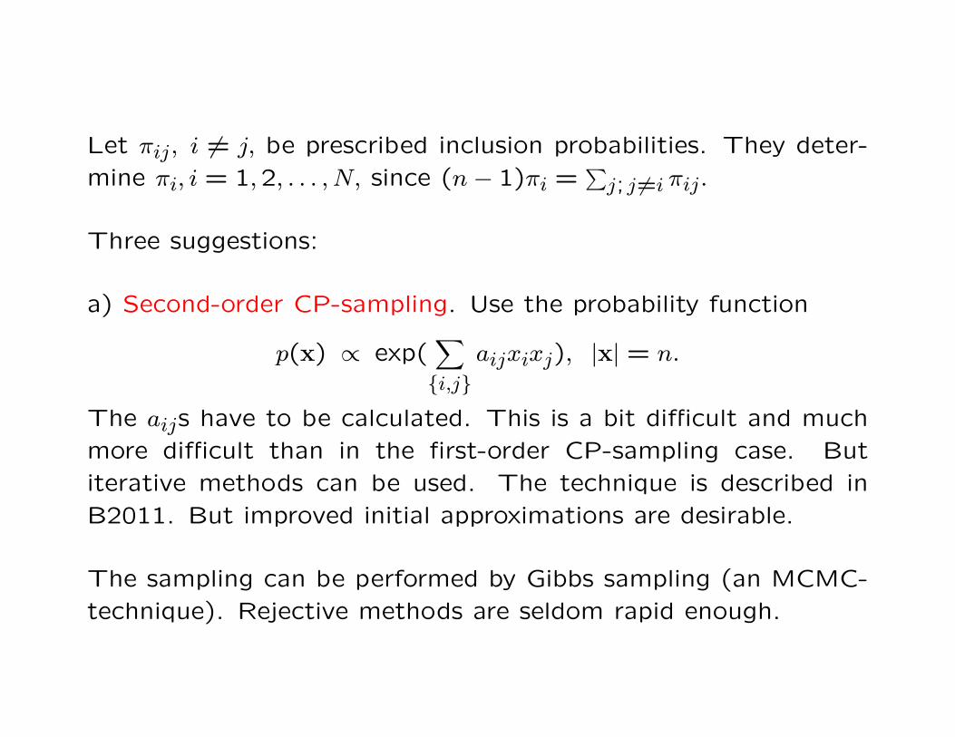
Let πij, i 6= j, be prescribed inclusion probabilities. They deter-

mine πi, i = 1,2, . . . , N, since (n− 1)πi =∑

j; j 6=i πij.

Three suggestions:

a) Second-order CP-sampling. Use the probability function

p(x) ∝ exp(∑{i,j}

aijxixj), |x| = n.

The aijs have to be calculated. This is a bit difficult and much

more difficult than in the first-order CP-sampling case. But

iterative methods can be used. The technique is described in

B2011. But improved initial approximations are desirable.

The sampling can be performed by Gibbs sampling (an MCMC-

technique). Rejective methods are seldom rapid enough.

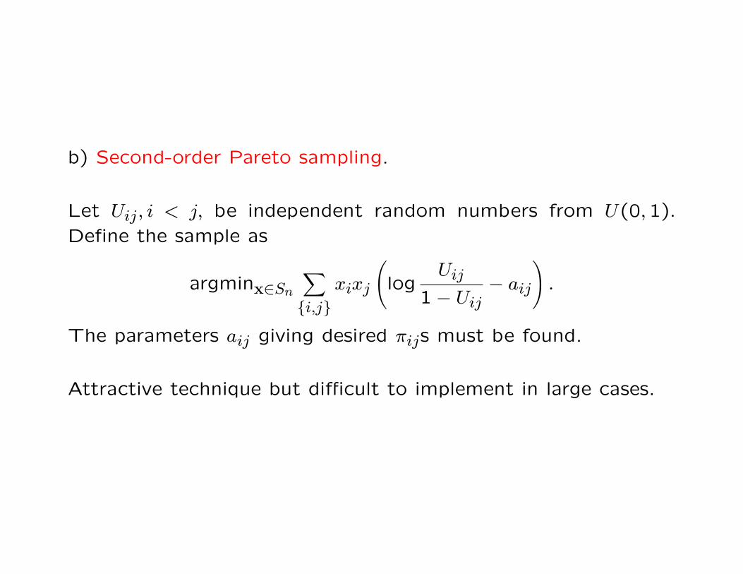
b) Second-order Pareto sampling.

Let Uij, i < j, be independent random numbers from U(0,1).

Define the sample as

argminx∈Sn

∑{i,j}

xixj

(log

Uij

1− Uij− aij

).

The parameters aij giving desired πijs must be found.

Attractive technique but difficult to implement in large cases.

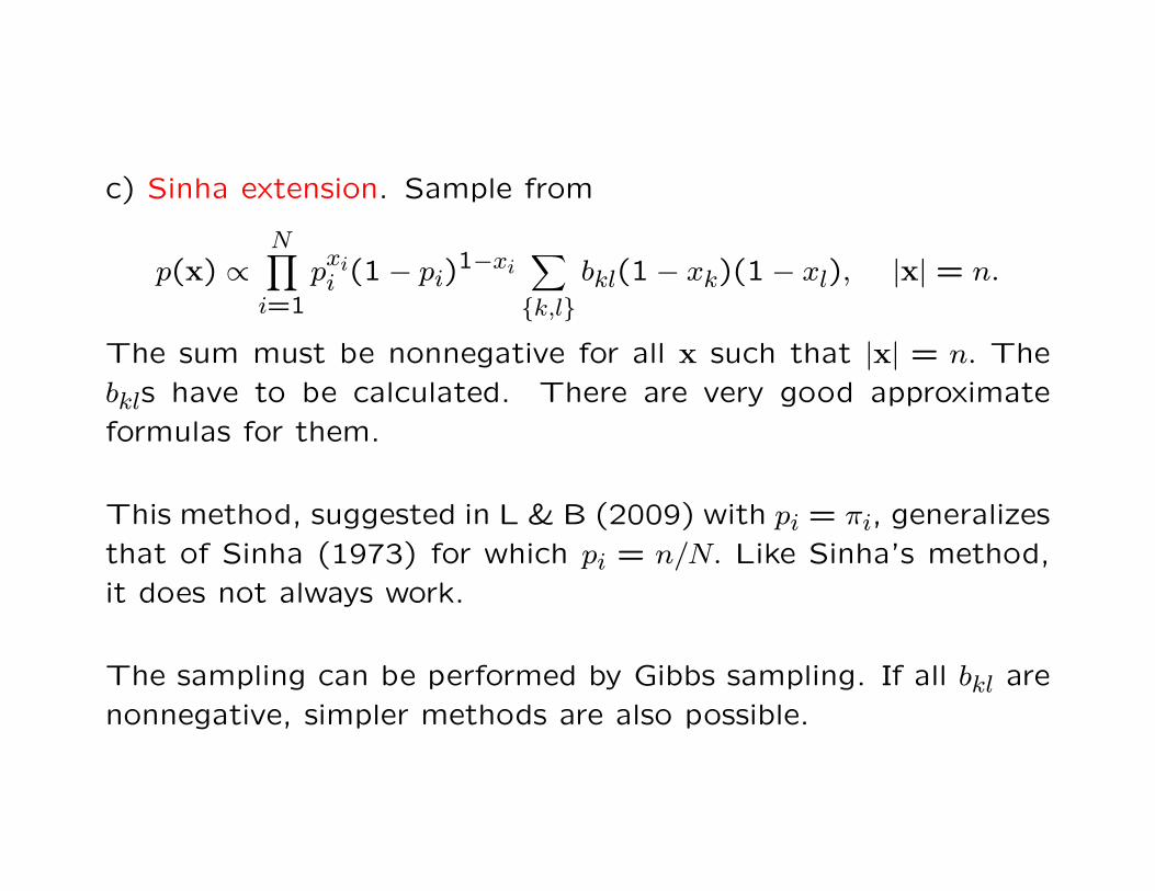
c) Sinha extension. Sample from

p(x) ∝N∏

i=1

pxii (1− pi)

1−xi∑{k,l}

bkl(1− xk)(1− xl), |x| = n.

The sum must be nonnegative for all x such that |x| = n. The

bkls have to be calculated. There are very good approximate

formulas for them.

This method, suggested in L & B (2009) with pi = πi, generalizes

that of Sinha (1973) for which pi = n/N. Like Sinha’s method,

it does not always work.

The sampling can be performed by Gibbs sampling. If all bkl are

nonnegative, simpler methods are also possible.

4. Conclusions

• Extended Sampford sampling (ESS), and variants thereof,

leads to a more continuous type of sampling and can be used

to change and improve common sampling practice. Variance

estimators can easily be produced.

• Balanced (restricted) Pareto sampling is an alternative to the

cube method by D & T (2004). It has the advantage that

it permits use of permanent random numbers.

• Methods for sampling with prescribed second-order inclusion

probabilities need further development to become practical.

5. References

Bondesson, L. (2010). Conditional and restricted Pareto sampling: two newmethods for unequal probability sampling. Scand. J. Statist. 37, 514-530.

” —— ” (2011). Sampling with prescribed second-order inclusion probabili-ties. Manuscript, 34 pages. Submitted.

” —— ” , Traat, I. & Lundqvist, A. (2006). Pareto sampling versus condi-tional Poisson and Sampford sampling. Scand. J. Statist. 33, 699-720.

” —— ” & Thorburn D. (2008). A list sequential sampling method suitablefor real time sampling. Scand. J. Statist. 35, 466-483.

” —— ” & Grafstrom, A. (2011). An extension of Sampfords method forunequal probability sampling. Scand. J. Statist. 38, 377-392.

Brewer, K.R.W. & Hanif, M. (1983). Sampling with unequal probabilities.Lecture Notes in Statistics, No. 15. Springer-Verlag, New York.

Chaudhuri, A. & Vos, J.W.E. (1988). Unified theory and strategies of surveysampling. North-Holland, Amsterdam.

Deville, J-C. & Tille, Y. (1998). Unequal probability sampling without re-placement through a splitting method. Biometrika 85, 89-101.

Deville, J-C. & Tille, Y. (2004). Efficient balanced sampling: The cubemethod. Biometrika, 91, 893-912.

Hajek, J. (1981). Sampling from a finite population. Marcel Dekker, NewYork.

Grafstrom, A. (2010). On Unequal Probability Sampling Designs. PhD-thesis, Dept of Math. and Math. Statist., Umea Univ.

Hanurav, T.V. (1966). Some aspects of unified sampling theory. Sankhya A28, 175-204.

Lundqvist, A. & Bondesson, L. (2009). On sampling with desired inclusionprobabilities of first and second order. Paper II in Lundqvist, A. (2009):Contributions to the theory of unequal probability sampling. PhD-thesis,Dept. of Mathematics and Mathematical Statistics, Umea University.

Meister, K. (2004). On methods for real time sampling and distributions insampling. Ph.D thesis, Dept. of Mathematical Statistics, Umea University,Umea.

Rosen, B. (1997). On sampling with probability proportional to size. J.Statist. Plann. Inference 62, 159-191.

Sampford, M.R. (1967). On sampling without replacement with unequalprobabilities of selection. Biometrika 54, 499-513.

Sarndal, C-E, Swensson, B. & Wretman, J. (1992). Model assisted surveysampling. Springer-Verlag, New York.

Sinha, B.K. (1973). On sampling schemes to realize preassigned sets ofinclusion probabilities of first two orders. Bull. Calcutta Statist. Assoc. 22,89-110.

Tille, Y. (2006). Sampling algorithms. Springer series in statistics. Springerscience + Business media, Inc., New York.

Traat, I., Bondesson, L. & Meister, K. (2004). Sampling design and sampleselection through distribution theory. J. Statist. Plann. Inference 123, 395-413.

Kadri Meister, Anders Lundqvist & Anton Grafstrom

Thanks for your attention!

Here this talk was prepared