Existence and regularity results for solutions of spectral ...
137
Existence and regularity results for solutions of spectral problems DerNaturwissenschaftlichenFakult¨at der Friedrich-Alexander-Universit¨ at Erlangen-N¨ urnberg und dem Dipartimento di Matematica “Felice Casorati” der Universit` a degli Studi di Pavia zur Erlangung des Doktorgrades Dr. rer. nat. Vorgelegt von Dario Mazzoleni aus Bergamo
Transcript of Existence and regularity results for solutions of spectral ...
Existence and regularity results for solutionsof spectral problems
Der Naturwissenschaftlichen Fakultat
der Friedrich-Alexander-Universitat Erlangen-Nurnberg
und
dem Dipartimento di Matematica “Felice Casorati”
der Universita degli Studi di Pavia
zur
Erlangung des Doktorgrades Dr. rer. nat.
Vorgelegt von
Dario Mazzoleni
aus Bergamo
2
Als Dissertation genehmigt
von der Naturwissenschaftlichen Fakultat
der Friedrich-Alexander-Universitat Erlangen-Nurnberg
Tag der mundlichen Prufung: 02.12.2014
Vorsitzender des Promotionsorgans: Jorn Wilms
Gutachter: Prof. Dr. Aldo Pratelli
Gutachter: Prof. Dr. Giuseppe Buttazzo
Gutachter: Prof. Dr. Dorin Bucur
3
Ai miei genitori,
a Valentina e a Stella

4
5
Abstract:
This Thesis is devoted to the study of some shape optimization problems for eigenvalues of
the Dirichlet Laplacian. More precisely we consider the minimum problem
minF (λ1(Ω), . . . , λk(Ω)) : Ω ⊂ RN , quasi-open, |Ω| = 1
,
with F : Rk → R increasing in each variable and lower semicontinuous.
The first result of the Thesis is a proof of the existence of an optimal set for such a prob-
lem, thus extending a well-known result due to Buttazzo and Dal Maso to the “unbounded”
setting. Moreover, under a slightly stronger assumption on F , it is possible to prove that all
the minimizers have a diameter uniformly bounded by a constant depending only on k,N (but
not on the functional). The main interest of this result is the very “elementary” techniques
that are used. In fact the key point consists in showing that it is always possible to choose a
minimizing sequence made of sets with uniformly bounded diameter, since getting rid of “long
tails” decreases the first k eigenvalues.
Then we focus on the study of the regularity of optimal sets, in particular a natural con-
jecture is that they should be open sets, at least. This kind of issue reveals to be quite hard to
solve. With a “direct” approach we can prove, in the two dimensional setting, that minimizers
for functionals like λ1(·) + · · ·+ λk(·) are open sets. Moreover we perform a finer analysis of the
eigenfunctions of optimal sets (in generic dimension), employing techniques from the regularity
of free boundary problems. In particular we prove that an optimal set Ω for the functional λk(·)has an eigenfunction, corresponding to the eigenvalue λk(Ω), which is Lipschitz continuous in
RN .
At last we study the connectedness of optimal sets for convex combinations of the first three
eigenvalues, and in particular we are able to prove that every minimizer for the problem
minαλ1(Ω) + (1− α)λ2(Ω) : Ω ⊂ RN , (quasi-)open, |Ω| = 1
,
is connected for all α ∈ (0, 1].
Sunto:
Questa Tesi tratta alcuni problemi di ottimizzazione di forma per autovalori del Laplaciano
con condizioni al bordo di Dirichlet omogenee. Piu precisamente consideriamo il problema di
minimo
minF (λ1(Ω), . . . , λk(Ω)) : Ω ⊂ RN , quasi-aperto, |Ω| = 1
,
ove F : Rk → R e un funzionale crescente in ciascuna variabile e semicontinuo inferiormente.
Il primo risultato della Tesi e una dimostrazione dell’esistenza di un insieme ottimale per
tale problema, che estende un ben noto risultato di Buttazzo e Dal Maso al caso “non limi-
tato”. Inoltre, sotto ipotesi leggermente piu forti per F , e possibile mostrare che tutti i minimi
6
hanno diametro uniformemente limitato da una costante che dipende solo da k,N (ma non dal
funzionale). Il principale interesse di questo risultato e il metodo di dimostrazione utilizzato,
che e molto “elementare”. Infatti il punto chiave consiste nel mostrare che e sempre possibile
prendere successioni minimizzanti composte da insiemi con diametro uniformemente limitato,
poiche eliminare delle “lunghe code” fa decrescere i primi k autovalori.
In seguito studiamo la regolarita degli insiemi ottimali, in particolare una naturale conget-
tura e che siano almeno aperti. Questo tipo di problema si rivela essere piuttosto difficile da
risolvere. Con un approccio “diretto” possiamo dimostrare, in due dimensioni, che i minimi
per funzionali come λ1(·) + · · · + λk(·) sono aperti. Inoltre analizziamo le autofunzioni degli
insiemi ottimali (in dimensione generica), utilizzando tecniche provenienti dalla teoria della re-
golarita per problemi con frontiera libera. In particolare, mostriamo che un insieme ottimo Ω
per il funzionale λk(·) ammette una autofunzione, corrispondente all’autovalore λk(Ω), che e
Lipschitziana in tutto RN .
Infine studiamo quando gli insiemi ottimali sono connessi per combinazioni convesse dei
primi tre autovalori e in particolare possiamo dimostrare che ogni minimo per il problema
minαλ1(Ω) + (1− α)λ2(Ω) : Ω ⊂ RN , (quasi-)aperto, |Ω| = 1
,
e connesso per ogni α ∈ (0, 1].
Zusammenfassung:
Diese Arbeit widmet sich der Untersuchung von Gestaltoptimierungsproblemen fur Eigen-
werte des Dirichlet-Laplace-Operators. Genauer gesagt betrachten wir das Minimierungsprob-
lem
minF (λ1(Ω), . . . , λk(Ω)) : Ω ⊂ RN , quasi-offen, |Ω| = 1
mit F : Rk → R wachsend in allen Variablen und unterhalbstetig.
Das erste Resultat ist der Existenzbeweis einer optimalen Menge fur ein solches Problem, was
ein bekanntes Resultat von Buttazzo und Dal Maso auf die “unbeschrankte” Situation erweitert.
Weiterhin ist es unter einer etwas starkeren Voraussetzung an F moglich zu zeigen, dass alle
Minimierer einen gleichmaßig durch eine Konstante beschrankten Durchmesser haben, wobei die
Konstante nur von k und N (jedoch nicht vom Funktional F ) abhangt. Das Bemerkenswerteste
an diesem Resultat sind die sehr “elementaren” Techniken die verwendet wurden. In der Tat ist
der entscheidende Punkt zu zeigen, dass es immer moglich ist, eine Minimalfolge von Mengen
mit gleichmaßig beschranktem Durchmesser auszuwahlen, da das Entfernen “langer Auslaufer”
die ersten k Eigenwerte verkleinert.
Danach konzentrieren wir uns auf die Untersuchung der Regularitat der optimalen Mengen.
Eine naturliche Vermutung dabei ist, dass diese zumindest offen sein sollten. Dies erweist
sich jedoch als recht schwierig zu beweisen. Mit einer “direkten” Vorgehensweise konnen wir
7
im zweidimensionalen Fall zeigen, dass Minimierer von Funktionalen wie λ1(·) + . . . + λk(·)offene Mengen sind. Daruber hinaus fuhren wir eine detailliertere Analyse der Eigenfunktionen
optimaler Mengen (allgemeiner Dimension) aus, wobei Techniken aus der Regularitatstheorie
freier Randwertprobleme zum Einsatz kommen. Insbesondere beweisen wir, dass eine optimale
Menge Ω fur das Funktional λk(·) eine Eigenfunktion zum Eigenwert λk(Ω) besitzt, welche
Lipschitz-stetig auf RN ist.
Abschließend untersuchen wir die Zusammenhangseigenschaften optimaler Mengen fur Kon-
vexkombinationen der ersten drei Eigenwerte. Genauer gelingt es uns dabei zu zeigen, dass jeder
Minimierer des Problems
minαλ1(Ω) + (1− α)λ2(Ω) : Ω ⊂ RN , quasi-offen, |Ω| = 1
zusammenhangend ist fur alle α ∈ (0, 1].

8
Contents
1 Introduction 11
2 Preliminaries and some existence results 19
2.1 Capacity, quasi-open sets and Sobolev spaces . . . . . . . . . . . . . . . . . . . . 19
2.2 PDEs and eigenvalues of elliptic operators . . . . . . . . . . . . . . . . . . . . . . 22
2.3 Extremum problems and bounds for eigenvalues . . . . . . . . . . . . . . . . . . . 26
2.4 γ-convergence and existence in a bounded box . . . . . . . . . . . . . . . . . . . . 32
2.5 Concentration compactness and subsolutions . . . . . . . . . . . . . . . . . . . . 35
3 Existence of minimizers in RN 39
3.1 Proof of Theorem 3.1 . . . . . . . . . . . . . . . . . . . . . . . . . . . . . . . . . . 39
3.1.1 Boundedness of the tails . . . . . . . . . . . . . . . . . . . . . . . . . . . . 40
3.1.2 Boundedness of the interior . . . . . . . . . . . . . . . . . . . . . . . . . . 51
3.1.3 Proof of Proposition 3.2 . . . . . . . . . . . . . . . . . . . . . . . . . . . . 57
3.2 Boundedness of all minimizers . . . . . . . . . . . . . . . . . . . . . . . . . . . . . 58
3.2.1 “Tails” . . . . . . . . . . . . . . . . . . . . . . . . . . . . . . . . . . . . . . 59
3.2.2 Interior . . . . . . . . . . . . . . . . . . . . . . . . . . . . . . . . . . . . . 62
3.2.3 Proof of Theorem 3.15 . . . . . . . . . . . . . . . . . . . . . . . . . . . . . 63
4 A two dimensional partial regularity result 65
4.1 Introduction and statement of the main Theorem . . . . . . . . . . . . . . . . . . 65
4.2 Proof of Theorem 4.2 . . . . . . . . . . . . . . . . . . . . . . . . . . . . . . . . . . 68
5 Lipschitz regularity of eigenfunctions 83
5.1 Preliminaries . . . . . . . . . . . . . . . . . . . . . . . . . . . . . . . . . . . . . . 83
5.2 Lipschitz continuity of energy quasi-minimizers . . . . . . . . . . . . . . . . . . . 86
5.3 Shape quasi-minimizers for Dirichlet eigenvalues . . . . . . . . . . . . . . . . . . 97
5.4 Shape supersolutions of spectral functionals . . . . . . . . . . . . . . . . . . . . . 101
5.5 Optimal sets for special functionals . . . . . . . . . . . . . . . . . . . . . . . . . . 106
9
10 CONTENTS
6 Connectedness of minimizers 111
6.1 Introduction . . . . . . . . . . . . . . . . . . . . . . . . . . . . . . . . . . . . . . . 111
6.2 Explicit computations of eigenvalues for balls . . . . . . . . . . . . . . . . . . . . 112
6.3 Statement of the main Theorems . . . . . . . . . . . . . . . . . . . . . . . . . . . 113
6.4 The general case . . . . . . . . . . . . . . . . . . . . . . . . . . . . . . . . . . . . 115
6.5 The two dimensional case . . . . . . . . . . . . . . . . . . . . . . . . . . . . . . . 126
6.5.1 Proof of Theorem 6.4 (a). . . . . . . . . . . . . . . . . . . . . . . . . . . . 131
6.5.2 Proof of Theorem 6.4 (b). . . . . . . . . . . . . . . . . . . . . . . . . . . . 132
Bibliography . . . . . . . . . . . . . . . . . . . . . . . . . . . . . . . . . . . . . . . . 133
Chapter 1
Introduction
Looking for optimal shapes is for sure one of the most fascinating topic of mathematics. This
is probably due to the many different fields of mathematics which are involved: spectral theory,
partial differential equations, calculus of variations, geometric measure theory, etc. Moreover,
as Buttazzo highlights in [24], a shape is something closer to human spirit than a function, and
maybe the big interest of mathematicians in shape optimization problems is motivated also by
this “philosophical” reason. The study of shapes from a mathematical point of view is a very
difficult subject and shape optimization problems are often, as Henrot writes in [38], very simple
to state but very hard to solve.
A very general shape optimization problem can be written in the following way:
min F(Ω) : Ω ∈ A, (1.1)
where A ⊂ P(RN ) denotes the family of admissible shapes and F : A → R is a “cost” functional.
In this wide setting, many well known topics fit: from isoperimetric problems to the Newton
problem of aerodynamical shapes, till spectral optimization for Schrodinger operators. Shapes
are very general geometric objects (manifolds, metric spaces, etc), but in this Thesis we focus
only on domains of the Euclidean space RN . The main issues regarding problem (1.1) are:
1. to prove the existence of a solution;
2. to describe the properties of optimal sets (e.g. openness, closedness, connectedness, con-
vexity);
3. to provide numerical approximations of solutions.
We address only the first two points in our work and we focus on the class of shape op-
timization problems involving eigenvalues of the Dirichlet Laplacian: in particular, we are in-
terested in the problem of existence of a solution, of its regularity and at last we study the
property of connectedness of minimizers in some peculiar case. More precisely, we choose
11
12 CHAPTER 1. INTRODUCTION
F(Ω) = F (λ1(Ω), . . . , λk(Ω)) and the general minimization problem that we consider is the
following:
minF (λ1(Ω), . . . , λk(Ω)) : Ω ⊂ RN , open, |Ω| ≤ 1
, (1.2)
where k,N ∈ N, | · | denotes the Lebesgue N -dimensional measure and we call λi the eigenvalues
of the Dirichlet Laplacian (counted with multiplicity). The bound on the measure is taken less
than or equal to 1 only for simplicity: with every other positive constant everything remains un-
changed. Moreover, since eigenvalues are decreasing with respect to set inclusion, it is equivalent
to consider the problem with the equality constraint.
This kind of optimization problems naturally arise in the study of many physical phenomena,
e.g. heat diffusion or wave propagation inside a domain Ω ⊂ RN , and the literature is very wide
(see [20, 38, 39, 24] for an overview), with many works in the last few years. Problem (1.2)
was studied first by Lord Rayleigh in his treatise The theory of sound of 1877 (see [48]), where
he focused on the case F = λ1 and he conjectured the unit ball to be the optimal set. This
was proved by Faber and Krahn (see [35, 43, 44]) in the 1920s, using techniques based on
spherical decreasing rearrangements. From that result, the case F = λ2 follows easily considering
the nodal domains: Krahn and Szego (see [43, 44, 49]) proved two disjoint equal balls of half
measure each to be optimal. The situation for k ≥ 3 becomes more complex and it is not known
what are the optimal shapes, up to now. As an example of the difficulties in finding explicit
minimizers, recent numerical results (see [4], [46]) shows that the minimizers for λ3 change with
the dimension. The only other functionals of eigenvalues for which the optimal shape is known
are λ1/λ2 and λ2/λ3: Ashbaugh and Benguria (see [7]) proved that the minimizers are the unit
ball and two equal disjoint balls of half measure each respectively.
Existence of optimal shapes. Since the search for explicit solutions did not give other
results, it is natural to study at least whether a minimizer for (1.2) exists, and this subject turns
out to be a difficult one, too. The main reason of difficulty is the lack of compactness for generic
sequences of open sets. Moreover it is not clear, given a converging sequence of open sets with
unit measure, whether the limit is a set at least in some suitable sense. The search for a “right”
notion of convergence in this setting was a main problem for many years. In the 1980s Dal Maso
and Mosco (see [31, 32]) proposed the notion of γ-convergence, which was the main tool used
by Buttazzo and Dal Maso in 1993 (see [26]) for proving a fundamental existence result for very
general functionals of eigenvalues, in the class of quasi-open1 sets inside a fixed bounded box.
More precisely, they fix, a priori, a bounded open set D ⊂ RN and consider a functional
F : Rk → R increasing in each variable and lower semicontinuous (l.s.c.). Then there exists a
minimizer for the problem:
min F (λ1(Ω), . . . , λk(Ω)) : Ω ⊂ D, quasi-open, |Ω| ≤ 1. (1.3)
1A quasi-open set is a superlevel of an H1 function.
13
The above result gives a definitive answer to the existence problem for very general class of
spectral functionals in a bounded ambient space (actually, it is sufficient to suppose D to have
finite measure in order to have the compact injection of H10 (D) in L2(D), as shown in [19]). The
extension of the result by Buttazzo and Dal Maso to generic domains in RN is a non trivial topic
because minimizing sequences, in principle, could have a significant portion of volume moving
to infinity.
A first result in the direction of existence in RN was obtained by Bucur and Henrot in 2000
(see [23]); they proved existence for λ3, using a concentration-compactness argument (see [18]).
Moreover, they showed that given k ≥ 1, if there exists a bounded minimizer for λj for all
j = 1, . . . , k − 1, then there exists a minimizer for λk and also for Lipschitz functionals of the
first k eigenvalues. Unfortunately, this boundedness hypothesis was not known even for λ3. In
a very recent result, Bucur (see [16]) was able to study the class of energy shape subsolutions
with techniques coming from the theory of free boundary and to prove, for them, boundedness
and finiteness of the perimeter. Since optimal sets for (1.2) can be proved to be energy shape
subsolutions, it is then possible to obtain existence for λk for all k.
At the same time, we gave in collaboration with Aldo Pratelli, an independent proof of
existence of a solution for problem (1.3) in RN (see [M4]), with the very same hypotheses of
Buttazzo and Dal Maso on F (increasing in each variable and l.s.c.). This different proof is more
“elementary” and involves neither a concentration-compactness argument nor the regularity of
energy shape subsolutions. The idea consists in showing that, given a minimizing sequence for
the problem,
minF (λ1(Ω), . . . , λk(Ω)) : Ω ⊂ RN , quasi-open, |Ω| = 1
, (1.4)
it is then possible to find a new one made of sets with diameter bounded by a constant depending
only on k,N and with all the first k eigenvalues not increased. This argument, roughly speaking,
works because sets with long “tails” must have some tiny section and hence they can not have
the first k eigenvalues very small. Moreover, with minor changes in the proof, it is also possible
to deduce that all minimizers for (1.4) are bounded, provided that F is weakly strictly increasing
(see [M3]).
In recent years, the existence of optimal sets was studied also for other kinds of shape
optimization problem involving eigenvalues of Dirichlet Laplacian. A first example is the case
of an internal constraint, that is,
minλk(Ω) : D ⊂ Ω ⊂ RN , quasi-open, |Ω| ≤ 1
,
where D is a fixed quasi open box with |D| ≤ 1. Bucur, Buttazzo and Velichkov in [22], using
a concentration compactness argument similar to the one in [18], proved existence of a solution
for k = 1, gave a characterization of the cases when k ≥ 2 and moreover proved some regularity
of the solutions.
It is also possible to consider spectral shape optimization problems with perimeter constraint
14 CHAPTER 1. INTRODUCTION
instead of volume constraint. This kind of problem was studied in the recent paper by De
Philippis and Velichkov [34], where they prove that there exists a minimizer for
minλk(Ω) : Ω ⊂ RN , measurable, P (Ω) ≤ 1
.
They use techniques to some extent analogous to those used by Bucur in [16], combining a
concentration compactness argument and the study of the regularity for perimeter shape subso-
lutions. The perimeter constraint turns out to have a better regularizing effect than the volume
constraint. In fact De Philippis and Velichkov are able to give many informations about regu-
larity of optimal shapes: first of all the optimal shapes are open, so the above problem has a
solution also among open sets.
Regularity of optimal shapes and of their eigenfunctions. The results exposed
above give a quite complete understanding for the problem of existence of minimizers for spectral
functionals involving eigenvalues of the Dirichlet Laplacian with a measure constraint. A further
question, arising from Buttazzo and Dal Maso Theorem, is the study of the regularity of optimal
sets or of the corresponding eigenfunctions. For example, a natural conjecture is that minimizers
for (1.3) and (1.4) are open sets and not only quasi-open. This is a quite difficult question, due to
the min-max nature of the eigenvalues and to the necessity of dealing with external perturbation
of sets. The only complete result in this field deals with the regularity of the free boundary of the
optimal set for λ1 inside a bounded box and was obtained by Briancon and Lamboley in [13]: in
that case the free boundary turns out to be smooth. On the other hand, at least in the bounded
setting, it is not always true the smoothness of a minimizer: in fact the optimal set for λ2 has
boundary not even Lipschitz, if the box is a sufficiently small rectangle. When working with
higher eigenvalues, many difficulties arise since the techniques developed by Alt and Caffarelli
for the study of the free boundary (see [2]) do not work for functionals defined through a min-
max procedure on H10 .
In Chapter 5 of the Thesis we present a result obtained in collaboration with Bucur, Pratelli
and Velichkov (see [M1]), in which we study the regularity of eigenfunctions on an optimal set
for
minλ1(Ω) + · · ·+ λk(Ω) : Ω ⊂ RN , (quasi-)open, |Ω| ≤ 1
, (1.5)
and we prove that the first k eigenfunctions are Lipschitz continuous in RN . Actually it is also
possible to provide regularity of eigenfunctions of optimal sets also for more general functionals,
but unfortunately, in the most interesting case of λk alone we are only able to prove that
there exists a Lipschitz eigenfunction corresponding to the kth eigenvalue. This does not imply
that an optimal set is open and this question remains one major conjecture in spectral shape
optimization.
We present in Chapter 4 of this Thesis also an “elementary” method that does not involve
free boundary techniques in order to prove the openness of optimal sets for problem (1.5) in
15
two dimensions. We do not obtain better results with this method, but we believe it is worth of
notice.
Connectedness of optimal shapes. In [M2], we deal with a different kind of problem
about connectedness of optimal sets for a spectral optimization problem. More precisely we
study, for a convex combination of the first three eigenvalues of the Dirichlet Laplacian, the
minimum problem
infαλ1(Ω) + βλ2(Ω) + (1− α− β)λ3(Ω) : Ω ⊂ RN , open, |Ω| ≤ 1, (1.6)
with α, β ∈ [0, 1] and α + β ≤ 1. Our aim is to investigate for which values of α, β all the
minimizers are connected. From Faber-Krahn inequality it follows that the unit ball is the
minimizer when α = 1 and β = 0. On the other hand, by the Krahn-Szego inequality, the
disjoint union of two equal balls of half measure each is the optimal set when α = 0, β = 1,
hence in this case the minimizer is disconnected.
The idea of studying such a convex combination arises from the inspiring paper by Wolf and
Keller [53], in which they proved that every minimizer for λ3 (that corresponds to α = β = 0)
must be connected in dimension N = 2 or 3. Their idea is quite simple and consists in studying
the best disconnected domain and to compare it with the ball, for which the values of eigenvalues
are known and depend only on the zeros of Bessel function.
The most important result that we obtain is to prove that every minimizer for the convex
combination
minαλ1(Ω) + (1− α)λ2(Ω) : Ω ⊂ RN , (quasi)-open, |Ω| ≤ 1
,
is connected in every dimension for α ∈ (0, 1]. Moreover we give some information for the other
cases, mostly in R2. A natural conjecture is that, in two dimensions, every minimizer for (1.6)
is connected unless α = 0 and β = 1. A recent numerical work by Kao and Osting (see [41])
supports the above conjecture and moreover suggests that the ball is an optimal set in all the
region α+ 2β ≤ 1.It is worth noticing that in the last few years many other numerical computations of the optimal
shapes for single lower eigenvalues have been done. In particular Oudet [46], Antunes and
Freitas [4] computed the optimal shapes for λk till k = 10 and k = 15, respectively. Their
computations suggest that only the optimal sets for λ2 and λ4 should be disconnected in the
two dimensional case. Moreover Berger and Oudet [11] proved that in R2 union of balls are
never optimal for λk if k ≥ 5.
Plan of the Thesis
In this thesis we will present the complete proofs only of original results obtained with our
contribution. For all the other results, we will give only the statements, sometimes a sketch of
the proof and the references where a detailed treatment can be found.
16 CHAPTER 1. INTRODUCTION
Chapter 2 is devoted to recall the basic concepts that we will need in the Thesis. First of
all we deal with the notions of capacity, quasi-open sets and Sobolev-like spaces. Then we recall
the definitions of eigenvalues for generic operators and we focus on the case of the Dirichlet
Laplacian. In Section 2.3 we treat some classical results about minimization of eigenvalues with
measure constraint and we present an useful bound. After that, we deal with the notion of
γ-convergence and the existence result by Buttazzo and Dal Maso, which is now classical. At
last, in Section 2.5, we deal with shape subsolutions and sketch the main idea of the existence
result [16] by Bucur.
In Chapter 3 we deal with the existence result presented in [M4], in particular we show that
it is always possible to apply the result of Buttazzo and Dal Maso also in the unbounded setting.
The proof is divided in two main steps: first we consider the tails of a regular set and then the
interior. Moreover, following [M3], we prove that all the optimal sets are uniformly bounded.
In Chapter 4 we start to study the regularity issue and we present a simple idea, strictly
related with the existence results just exposed, that gives some informations about the regularity
of optimal sets in two dimensions. In particular, we study what can be done if an optimal set
has “holes too small”. This approach allows also to understand what are the main difficulties
in proving a regularity result.
Chapter 5 is devoted to the presentation of the results of Lipschitz regularity for eigenfunc-
tions of optimal sets obtained in [M1]. First of all, we recall the techniques used by Briancon,
Hayouni and Pierre [14] for proving Lipschitz regularity of the energy function. Then we study
how to apply these techniques to shape quasi-minimizers for Dirichlet eigenvalues and at last we
deal with shape supersolutions and prove the Lipschitz regularity for eigenfunctions on optimal
domains. We also show for which functionals the Lipschitz regularity of eigenfunctions gives
informations about the openness of an optimal set.
At last, in Chapter 6 we deal with the question of connectedness of optimal sets for convex
combinations of the first three eigenvalues, following [M2]. More precisely, after recalling the
values of eigenvalues for balls, we first deal with the N -dimensional case and then give more
informations in two dimensions.
17
Table of notations
N,R space of natural and real numbers respectively
P(E) the power set of E
Hs s-dimensional Hausdorff measure
dimH(E) Hausdorff dimension of a set E
LN (E) = |E| N -dimensional Lebesgue measure of a set E
cap (E) (H1-)capacity of a set E
P (E; Ω) distributional perimeter of a set E inside Ω
〈·, ·〉 duality in H10
(·, ·) scalar product in a generic Hilbert space H
ωN N -dimensional Lebesgue measure of the unit ball in RN
CN constant depending only on the dimension N
E∆F symmetric difference between the sets E,F ⊆ RN
R(u,D) Rayleigh quotient of the function u in the domain D
∆ Laplace operator
div divergence operator
∂Ω topological boundary of the set Ω ⊆ RN
tΩ homothety of ratio t > 0 of a set Ω
X ′ topological dual of a Banach space X
λi i-th eigenvalue for −∆ with zero Dirichlet boundary conditions
ui i-th eigenfunction corresponding to the eigenvalue λi
Br(x) ball in RN of radius r ≥ 0 and centered in x
B ball in RN with measure 1
Θ disjoint union of two balls in RN of measure 12 each
M0(D) the class of capacitary measures on D
Aµ regular set of a measure µ
Rµ, RΩ resolvent operator associated to a measure µ or a set Ω
S class of measurable sets with finite Lebesgue measure
A(D) class of quasi-open sets Ω ⊂ D with |Ω| = 1
L(X) space of linear and continuous functional defined in a Banach space X
Jm m-th Bessel function
jm,k k-th zero of the Bessel function Jm
−∫A u average integral of the function u over the set A
l.s.c. lower semicontinuous
a.e. almost everywhere
q.e. quasi everywhere
18 CHAPTER 1. INTRODUCTION
Acknowledgments
After three years of “research”, there are really many people with whom I came in contact for
scientific reasons. Sometimes it was just for chatting about mathematics, in other cases it was
a full-time collaboration. Anyway my Thesis is really influenced by all these relations, that
improved greatly my human and mathematical knowledge.
First of all I have to thank my advisor Aldo Pratelli, whose deep insight in every corner of
Mathematical Analysis is really incredible. Working with him is for me a big honor, and I owe
him almost all of what I did in this Thesis and of what I learned of Mathematics in these three
years.
I have to thank a lot Bozhidar Velichkov, who helped me understand how to use the regularity
techniques for free boundary problems in this spectral shape optimization setting, and much
more. A great thanks goes to Dorin Bucur, for the suggestions and ideas that gave me and that
I hope to develop completely very soon. I want to thank Mette Iversen, for the work together
that is presented in Chapter 6, and Michiel van den Berg for putting us in contact.
There are then a lot of colleagues to thank for the discussions together: Giovanni Franzina,
Florian Zeisler (with huge gratitude for correcting the abstract in german), Emanuela Radici
and all the people from Erlangen that made me enjoy so much the time there.
A huge thanks goes also to Giuseppe Savare and Gian Pietro Pirola for supporting me in the
hard task of making the cotutelle agreement work and for answering kindly to the tons of email
I sent them.
I want then to thank all the people who were close to me during these years (and much
longer) with their mind and heart. First of all my family, who helped me in every choice and
without whom i would have never arrived at this point. I warmly thank Gabri and Paolo, for
being a second family for me. I thank all my friends from Bergamo and Pavia and Erlangen for
all the nice time that we spent (spend and will spend) together, and for being always ready to
help me when I needed support. At last, I can only say kheili, kheili mamnun to Hana (and to
the Iranian community of Erlangen), for the nice time together.
Chapter 2
Preliminaries and some existence
results
This Chapter is devoted to briefly introduce the reader to the main tools of spectral shape
optimization, which will be used throughout the Thesis. First, we deal with capacity, quasi-
open sets, generalized Sobolev spaces and classical extremum problems for eigenvalues. Then,
we enter more into details and we treat some recent fundamental existence results in shape
optimization. More precisely in Section 2.4 we introduce the γ-convergence and the existence
result by Buttazzo and Dal Maso [26]. Then in Section 2.5, we sketch the approach used by
Bucur [16] for proving existence in unbounded regions.
2.1 Capacity, quasi-open sets and Sobolev spaces
We need to recall the definition of capacity, which is very important in the study of problems
involving the space H10 , hence also for the study of eigenvalues of the Dirichlet Laplacian. For
more details we refer to [39].
Definition 2.1. Given a compact set K ⊂ RN , we define
cap (K) := inf‖v‖2H1(RN ) : v ∈ C∞c (RN ), v ≥ 1 in a neighborhood of K
.
Then, for an open set Ω ⊂ RN ,
cap (Ω) := sup cap (K) : K compact, K ⊂ Ω.
At last, for a generic measurable set E ⊂ RN ,
cap (E) := inf cap (Ω) : Ω open, Ω ⊃ E.
The last definition is well-posed, since it is easy to prove that for every compact set K ⊂ RN ,
it is cap (K) = inf cap (Ω) : Ω open, Ω ⊃ K. Moreover, it is possible to give the following
19
20 CHAPTER 2. PRELIMINARIES AND SOME EXISTENCE RESULTS
characterization of the capacity: for all measurable set E ⊂ RN ,
cap (E) = inf‖v‖2H1(RN ) : v ∈ H1(RN ), v ≥ 1 in a neighborhood of E
.
One can also consider the relative capacity inside a box, with analogous definitions, which can
be characterized as follows. Given an open, bounded set D ⊂ RN and a measurable set E ⊂ RN ,
the relative capacity is:
capD(E) = inf‖v‖2H1(D) : v ∈ H1(D), v ≥ 1 in a neighborhood of E
.
Mostly we are interested in sets with zero capacity, and it is immediate to check that cap (E) = 0
if and only if capD(E) = 0, for any suitable D ⊃ E.
Remark 2.2. It is clear from the definition that if cap (E) = 0, then |E| = 0. The opposite
implication is false, for example a segment in R2 has zero Lebesgue measure, but positive capacity.
In general, given E ⊂ RN , if dimH(E) ∈ [N − 1, N), then cap (E) > 0 and |E| = 0, while if
dimH(E) ≤ N − 2, then also cap (E) = 0.
We summarize some easy and useful properties of capacity.
(1) (Monotonicity) If E ⊂ F , then cap (E) ≤ cap (F );
(2) (Subadditivity) For all E,F we have cap (E ∩ F ) + cap (E ∪ F ) ≤ cap (E) + cap (F ).
(3) Given a family of disjoints sets (En)n∈N, then cap (∪En) ≤∑
cap (En).
(4) Given an increasing sequence of sets (En)n∈N, then cap (∪En) = limn→∞ cap (En).
(5) Given a decreasing sequence of compact sets (Kn)n∈N, then cap (∩Kn) = limn→∞ cap (Kn).
We say that a property P holds quasi everywhere (q.e.) if the set for which the property
does not hold has zero capacity, while we keep the usual terminology of almost everywhere (a.e.)
in the case of Lebesgue measure.
Remark 2.3. In the whole Thesis we consider sets defined up to zero capacity, hence also
notions such as connectedness should be intended in this acception.
Two very important notions related to the concept of capacity are the ones of quasi-open
set and quasi-continuous function, which will be fundamental throughout the Thesis.
Definition 2.4. We say that a set Ω ⊂ RN is quasi-open if for all ε > 0 there exists an open
set Ωε such that cap (Ω∆Ωε) < ε.
We call u : RN → R quasi-continuous if for all ε > 0 there exists an open set ωε such that
cap (ωε) < ε and the restriction of u to RN \ ωε is continuous.
2.1. CAPACITY, QUASI-OPEN SETS AND SOBOLEV SPACES 21
Every function u ∈ H1(RN ) has a quasi-continuous representative, which is unique up to
equality q.e. and can be defined in the following way:
∀x ∈ RN , u(x) := limr→0−∫Br(x)
u(y) dy.
In general, we will consider always the quasi-continuous representative of H1 functions and write
u instead of u. A key relation between these concepts is that, given u : RN → R quasi-continuous
and α ∈ R, then the set u > α is quasi-open. In fact, by definition, there exists, for all ε > 0,
an open set ωε, with cap (ωε) ≤ ε, such that u|ωcε is continuous. In particular, there are open
sets (Ωε) such that u > α ∩ ωcε = Ωε, that is equivalent to say that u > α ∪ ωε = Ωε ∪ ωε,which is an open set for all ε > 0.
We can then say that superlevels of H1 functions are quasi-open sets and this fact will be crucial
in the existence Theorem by Buttazzo and Dal Maso. Moreover for each quasi-open set Ω there
is a quasi-continuous function u ∈ H1(RN ) such that Ω = u > 0. It is clear that every open
set is quasi-open, and obviously one can add to an open set some pieces with zero capacity and
obtain a quasi-open set. But since quasi-open sets are defined up to sets with zero capacity this
is not really a new set. For an example of a quasi-open set which is not equivalent to an open
set see [39, Exercice 3.6].
In view of the above concepts, we can give a new definition of the space H10 , which is
meaningful also for a measurable set E ⊂ RN ,
H10 (E) :=
u ∈ H1(RN ) : u = 0 q.e. in RN \ E
. (2.1)
The extension of the space H1 to measurable sets is crucial, because, in order to obtain existence
results, it is very often necessary to work not only with open sets. We summarize some important
properties in the following lemma (a proof can be found in [39, Chapter 3]).
Lemma 2.5. (1) For a generic open set Ω, H10 (Ω) coincide with the usual definition as closure
of the smooth functions with compact support in Ω, that is C∞c (Ω), with respect to the H1
norm.
(2) For every measurable set E ⊂ RN there exists a quasi-open set ΩE such that H10 (E) =
H10 (ΩE).
(3) From the properties above we can deduce that if Ω is a quasi-open set with positive capacity,
then H10 (Ω) 6= 0, and hence |Ω| > 0.
Another possible extension of Sobolev spaces to measurable sets is given by the notion of Sobolev-
like space, which is employed mostly in Chapter 5. For any measurable set E ⊂ RN we define
H10 (E) :=
u ∈ H1(RN ) : u = 0 a.e. in RN \ E
. (2.2)
It is clear that the definition does not coincide in general with the one given in (2.1), not even
for open set: for example one can consider a ball minus a hyperplane passing through its center.
22 CHAPTER 2. PRELIMINARIES AND SOME EXISTENCE RESULTS
It is always true the obvious inclusion H10 (E) ⊆ H1
0 (E) and equality can be proved for open
sets with Lipschitz boundary (see [34]). Moreover, for all measurable E, there exists always a
quasi-open set ΩE ⊂ E such that
H10 (ΩE) = H1
0 (E).
Since H10 (E) is separable, it is sufficient to consider ΩE :=
⋃n∈N un 6= 0, where unn∈N is a
dense sequence in H10 (E).
2.2 PDEs and eigenvalues of elliptic operators
First of all we deal with the eigenvalues of general operators defined on Hilbert spaces. We
remind that, given a separable Hilbert space H with scalar product (·, ·) and a linear operator
R : H → H, we say that
• R is positive if (Rx, x) ≥ 0 for all x ∈ H,
• R is self-adjoint if (Rx, y) = (x,Ry) for all x, y ∈ H,
• R is compact if the image of a bounded set has compact closure in H.
We can summarize the main informations about eigenvalues in the following theorem (see, for
example, [38, Chapter 1]).
Theorem 2.6. Let H be a separable Hilbert space and R : H → H be a positive, self-adjoint and
positive operator. Then there exists a nonincreasing sequence of positive eigenvalues converging
to zero
0 ≤ · · · ≤ Λk+1(R) ≤ Λk(R) ≤ · · · ≤ Λ1(R),
and a sequence of normalized eigenvectors (xk)k, which are a basis for H and satisfy:
Rxk = Λk(R)xk, ∀k ∈ N.
Moreover the eigenvalues satisfy the so called Courant-Fisher and max-min formulas:
Λk(R) = minφ1,...,φk−1∈H
max
φ∈〈φ1,...,φk−1〉⊥
(Rφ, φ)
(φ, φ)
Λk(R) = max
Hk
min
φ∈Hk, (φ,φ)=1(Rφ,Rφ)
,
where the last maximum is over subspaces Hk ⊂ H of dimension k.
We want to focus on a special class of operators, related to capacitary measures. A positive
Borel measure is called capacitary if, for all measurable set E, cap (E) = 0 implies µ(E) = 0.
First of all, given µ ∈M0(RN ), we define its regular set Aµ (see [20, Chapter 4]) as the union of
2.2. PDES AND EIGENVALUES OF ELLIPTIC OPERATORS 23
all open sets A ⊂ RN such that µ(A) <∞. If Aµ has finite measure, we define Rµ the resolvent
operator associated to µ as:
Rµ : L2(RN )→ L2(RN ), Rµ(f) = u,
where u is the solution of
minv∈H1(RN )∩L2
µ(RN )
∫RN|Dv|2 +
∫RN
v2 dµ−∫RN
vf
,
where we call L2µ(RN ) :=
u ∈ L2(RN ) :
∫u2 dµ <∞
. Since |Aµ| < ∞, then H1
0 (Aµ) is
compactly embedded in L2(Aµ), hence Rµ is well defined, compact, positive and self-adjoint.
We are then able to define the eigenvalues associated to the measure µ, that is, eigenvalues of
the elliptic operator −∆ + µI, as
λk(µ) =1
Λk(Rµ),
so they form a positive nondecreasing sequence diverging to infinity as k → ∞. The Rayleigh
formula can be now read as
λk(µ) = minEk
maxv∈Ek
∫|Dv|2 +
∫v2 dµ∫
v2
,
where the minimum is over the k-dimensional subspaces of H1(RN ) ∩ L2µ(RN ).
We are interested, in this Thesis, mostly in eigenvalues of Dirichlet Laplacian on a open (or
quasi-open) subset of RN . In order to reduce the above machinery to this easier case, for every
(quasi-)open set Ω of finite volume |Ω|, we consider the measure
µΩ(E) =
0, if cap (E \ Ω) = 0,
+∞, if cap (E \ Ω) > 0,(2.3)
and we define λk(Ω) := λk(µΩ), observing that H1(RN ) ∩ L2µΩ
(RN ) = H10 (Ω). We remark that
this coincide with the usual definition of the kth eigenvalue of the Dirichlet Laplacian (counted
with multiplicity) as the kth element of the spectrum of the Dirichlet Laplacian, which is discrete
since |Ω| <∞ (see [36, 38]). In order to stress this equivalence, first of all we recall few definitions
about elliptic PDEs, which will also be used in the whole Thesis. Given Ω ⊂ RN a set of finite
measure and a function f ∈ L2(Ω), we say that u ∈ H1(RN ) satisfies the equation−∆u = f in Ω,
u ∈ H10 (Ω),
if for every v ∈ H10 (Ω) we have 〈∆u+ f, v〉 = 0, where we set
〈∆u+ f, v〉 := −∫RN
Du ·Dv +
∫RN
fv.
With the definition above in mind, we can say that λk(Ω) is the kth smaller number such that
there exists a function uk ∈ H10 (Ω) which satisfies
−∆uk = λk(Ω)uk in Ω,
24 CHAPTER 2. PRELIMINARIES AND SOME EXISTENCE RESULTS
and uk is called eigenfunction corresponding to λk(Ω). For sake of simplicity we always consider
the eigenfunctions with unit L2 norm, which is clearly possible up to rescaling. In this case the
min-max formula takes the form:
λk(Ω) = min
Ek ⊂H10 (Ω),
subspace of dimension k
maxv∈Ek\0
||Dv||2L(Ω)
||v||2L2(Ω)
. (2.4)
In particular, the minimum is achieved choosing Ek the space spanned by the first k eigenfunc-
tions u1, . . . , uk and the above ratio is called the Rayleigh quotient ; we denote it by
R(u,Ω) :=||Du||2
L(Ω)
||u||2L2(Ω)
.
In the case of measures corresponding to a set we call the resolvent operator RΩ := RµΩ and we
note that for all f ∈ L2(RN ),
RΩ(f) = arg min
1
2
∫RN|Du|2 −
∫RN
uf : u ∈ H10 (Ω)
.
We now list some important properties of eigenvalues of Dirichlet Laplacian, for the proofs
one can refer to [20]. We remind that given t > 0 and a set Ω, we use the notation tΩ :=
tx : x ∈ Ω .
Lemma 2.7. The following properties hold.
(1) (Monotonicity) Given Ω1,Ω2 ⊂ RN (quasi-)open set with finite measure, if Ω1 ⊆ Ω2, then
for all k ∈ N, λk(Ω2) ≤ λk(Ω1).
(2) (Scaling) Given Ω ⊂ RN a (quasi-)open set and t > 0, then for all k ∈ N, λk(tΩ) =
t−2λk(Ω).
(3) The first eigenfunction is strictly positive on the connected component on which is supported,
and it is zero on all the other components, if any.
Remark 2.8. Thanks to the scaling properties of eigenvalues the following minimum problems
are equivalent (for every k ∈ N):
min λk(Ω), |Ω| = 1, min λk(Ω), |Ω| ≤ 1, min|Ω|2/Nλk(Ω)
,
and we will use all the different formulations. It is worth noticing that in the last formulation
we have no more bound on the measure, and the quantity Ω 7→ |Ω|2/Nλk(Ω) is invariant under
homothety.
2.2. PDES AND EIGENVALUES OF ELLIPTIC OPERATORS 25
Remark 2.9. When Ω is disconnected, for example if it has two connected components Ω1 and
Ω2, we obtain the eigenvalues of Ω by collecting and reordering the eigenvalues of each connected
component
λ1(Ω) = min λ1(Ω1);λ1(Ω2)
λ2(Ω) = min
max λ1(Ω1);λ1(Ω2);λ2(Ω1);λ2(Ω2),
and so on. More generally we can always choose every eigenfunction of a disconnected open
set to vanish on all but one connected component of Ω. In fact, given λk, k ≥ 1, there exists
a connected component ω ⊂ Ω and an index i ≤ k, such that λk(Ω) = λi(ω). Hence we can
choose uk to be the eigenfunction linked to λi(ω), and we can extend it to zero on Ω \ ω. In
particular, when Ω is made by two equal connected components, we will have λ1(Ω) = λ2(Ω):
the first eigenvalue is double.
Another important property is about the eigenfunctions of the Dirichlet Laplacian, which
have the following bound in L∞ (for a proof we refer to [33]):
‖uk‖L∞ ≤ e1/8πλk(Ω)N/4, (2.5)
for every k ∈ N. This fact will be fundamental in Chapter 5, in order to use classical results
about PDEs with bounded data.
We conclude the Section with few words about eigenvalues on Sobolev-like spaces. One can
define the eigenvalues of the Dirichlet Laplacian on the linear subspace H10 (Ω) ⊆ H1(RN ). In
general, given a closed linear subspace H of H1(RN ), which is compactly embedded in L2(RN ),
one defines the spectrum of the Dirichlet Laplacian on H as (λ1(H), . . . , λk(H), . . . ), where the
kth eigenvalue is
λk(H) := minEk
maxu∈Ek\0
∫|Du|2 dx∫u2 dx
, (2.6)
and the minimum ranges over all k-dimensional subspaces Ek of H.
Given a measurable set E with finite measure and k ∈ N, then λk(Ω) = λk
(H1
0 (E))
and
there is a sequence of eigenfunctions uk ∈ H10 (E) orthonormal in L2 and satisfying the equation
−∆uk = λk(Ω)uk in Ω.
It is then clear that λk(H10 (E)) = λk(ΩE) ≥ λk(E) for some quasi-open set ΩE ⊂ E. Hence,
thanks to the monotonicity of eigenvalues w.r.t set inclusion, it is equivalent to study the mini-
mization problem
minF (λ1(E), . . . , λk(E)) : E ⊂ RN , |E| ≤ 1
,
in the class of quasi-open sets or in the family of measurable sets associated to H10 , up to
suppose the functional F to be increasing in each variable. We will use this new definition of
26 CHAPTER 2. PRELIMINARIES AND SOME EXISTENCE RESULTS
λk in Chapter 5 for the following reason. If a set of finite measure E∗ is minimal with respect
to exterior perturbations (and this is what we need to study the regularity issue), that is,
F(λ1(H1
0 (E∗)), . . . , λk(H10 (E∗))
)≤ F
(λ1(H1
0 (E)), . . . , λk(H10 (E))
)+ |E \ E∗|, ∀E ⊃ E∗,
then, for every ε > 0, E∗ is the unique solution of
minF(λ1(H1
0 (E)), . . . , λk(H10 (E))
)+ (1 + ε)|E| : E∗ ⊂ E ⊂ RN
. (2.7)
In fact, if E∗∗ is another solution of (2.7), then |E∗∆E∗∗| = 0, and so H10 (E∗) = H1
0 (E∗∗).
Remark 2.10. In the Thesis we focus only on Dirichlet boundary condition for the Laplacian,
but there are other common choices of boundary conditions that lead to completely different
problems (for more references one can look at the books [39, 20, 38]). One key property of the
Dirichlet boundary conditions is the monotonicity of eigenvalues with respect to inclusion, which
is false for the other conditions. In particular, a real number µ and a function u ∈ H1(RN ) are
an eigenvalue and the corresponding eigenfunction of the Neumann Laplacian if they solve (in
the weak formulation) −∆u = µu, in Ω,
∂u∂ν = 0, on ∂Ω.
More in general, given a, b ∈ [0, 1], the so called Robin boundary conditions reads as:−∆u = ρu, in Ω,
au+ b∂u∂ν = 0, on ∂Ω.
We observe that Robin conditions includes the others: for a = 1, b = 0 we find again the
Dirichlet boundary conditions, while for a = 0, b = 1 we obtain the Neumann one.
2.3 Extremum problems and bounds for eigenvalues of the Dirich-
let Laplacian
In this Section we consider classical minimum problems for eigenvalues of the Dirichlet Laplacian.
More precisely, one looks for a set (a “shape”) that minimize a single eigenvalue or a function of
eigenvalues. Due to the monotonicity, a constraint on the admissible sets is needed, otherwise
the minimization is not interesting. The most studied case is the one of volume constraint, but
in the last years also the perimeter constraint was investigated (see [34]). This kind of shape
optimization problem, in a general situation, can be written as
minF (λ1(Ω), . . . , λk(Ω)) : Ω ⊂ RN , (quasi-)open, |Ω| = 1
, (2.8)
and here we treat the few cases in which it is possible to find an explicit solution, considering
first the minimization of single eigenvalues, that is, F (λ1, . . . , λk) = λk, k ∈ N.
2.3. EXTREMUM PROBLEMS AND BOUNDS FOR EIGENVALUES 27
The minimization of λ1 was the first problem to be studied: Lord Rayleigh conjectured
the ball to be a minimizer in [48], and in the 1920s Faber and Krahn eventually proved his
conjecture to be true (see [35, 43, 44]), using spherical decreasing rearrangements. The so called
Faber-Krahn inequality states, in a scale invariant form,
λ1(Ω) ≥ λ1(B)
(|B||Ω|
)2/N
, for all open sets of finite measure Ω ⊂ RN , (2.9)
where B is the ball of unit measure in RN , and with equality if and only if Ω is any ball (up to
sets of capacity zero). Analogously, as a minimum problem:
λ1(B) = minλ1(Ω), : Ω ⊂ RN , open, |Ω| ≤ 1
.
The minimization of λ2 was implicitly solved in Krahn’s works (see [43, 44]) and then
rediscovered independently by Hong [40] and Szego [49] in the 1950s. In this case, studying the
nodal sets of the first two eigenfunctions, one can prove two disjoint equal balls to be optimal.
More precisely, in a scale invariant form, the (Hong-)Krahn-Szego inequality asserts that
λ2(Ω) ≥ 22/Nλ1(B)
(|B||Ω|
)2/N
, for all open sets of finite measure Ω ⊂ RN , (2.10)
with equality if and only if Ω is any disjoint union of two balls of equal measure. Equivalently,
it is
λ2(Θ) = minλ2(Ω), : Ω ⊂ RN , open, |Ω| ≤ 1
,
where we denote the union of two disjoint balls each of half measure by Θ.
Unfortunately explicit minimizers for λk, k ≥ 3, are not known and there is numerical
evidence, at least for λ3, that the optimal set should not be the same set in all dimensions
(see [4, 11]). For the interested reader we recall here some major conjectures about optimal sets
for single eigenvalues.
(1) The ball is optimal for λ3 in two dimensions,
(2) Three disjoint balls of equal volume are optimal for λ3 in dimension N ≥ 4,
(3) The optimal set for λ4 in two dimensions is made by two disjoint balls B1, B2 such that
λ3(B1) = λ1(B2),
(4) The ball of RN is optimal for λN+1 for all N ≥ 3.
It is worth noticing that minimizers for single eigenvalues are not always balls or union of balls:
Wolf and Keller proved in [53] that, for the minimization of λ13, the optimal union of rectangles
is a better candidate than the optimal union of balls in R2. Moreover Berger and Oudet [11], in
a very recent paper, proved that for k ≥ 5 the optimal set for λk in two dimensions is never a
union of balls.
28 CHAPTER 2. PRELIMINARIES AND SOME EXISTENCE RESULTS
The only other functionals for which the optimal sets are known are λ1/λ2 and λ2/λ3, thanks
to the works by Ashbaugh and Benguria [7, 8], who solved a conjecture by Payne, Polya and
Weinberger [47]. We present them in their original form as maximization results.
Theorem 2.11. The ball maximizes the ratio λ2/λ1, that is:
λ2(Ω)
λ1(Ω)≤ λ2(B)
λ1(B)for all open sets of finite measure Ω ⊂ RN . (2.11)
Moreover two equal disjoint balls maximize the ratio λ3/λ2, hence
λ3(Ω)
λ2(Ω)≤ λ3(Θ)
λ2(Θ)=λ2(B)
λ1(B)for all open sets of finite measure Ω ⊂ RN . (2.12)
In other words, the ball minimize λ1/λ2 and two equal disjoint balls minimize λ2/λ3.
At last we present an easy and well-known inequality that can be seen as an extension (even
if rougher) of the results by Ashbaugh and Benguria: in particular we have that the functional
λk/λ1 is bounded for all k ∈ N. This will be very useful in Chapter 3. We present here a simple
new proof given in [M4, Appendix], while another proof can be found in [6].
Theorem 2.12. There exists a constant M = M(k,N) such that for every (quasi-)open set one
hasλk(Ω)
λ1(Ω)≤M.
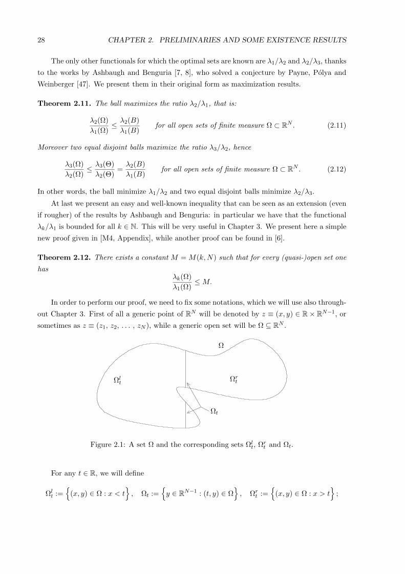
In order to perform our proof, we need to fix some notations, which we will use also through-
out Chapter 3. First of all a generic point of RN will be denoted by z ≡ (x, y) ∈ R× RN−1, or
sometimes as z ≡ (z1, z2, . . . , zN ), while a generic open set will be Ω ⊆ RN .
Ω
ΩrtΩl
t
Ωt
Figure 2.1: A set Ω and the corresponding sets Ωlt, Ωr
t and Ωt.
For any t ∈ R, we will define
Ωlt :=
(x, y) ∈ Ω : x < t
, Ωt :=
y ∈ RN−1 : (t, y) ∈ Ω
, Ωr
t :=
(x, y) ∈ Ω : x > t
;
2.3. EXTREMUM PROBLEMS AND BOUNDS FOR EIGENVALUES 29
notice that Ωlt and Ωr
t are subsets of RN , while Ωt is a subset of RN−1. Figure 2.1 shows an
example of a generic set Ω with Ωlt, Ωr
t and Ωt. On the other hand, given 0 ≤ m ≤ |Ω| and
0 ≤ m1 ≤ m2 ≤ |Ω|, we define the level τ(Ω,m) ∈ R and the width W (Ω,m1,m2) as
τ(Ω,m) := inft ∈ R :
∣∣Ωlt
∣∣ ≥ m , W (Ω,m1,m2) := τ(Ω,m2)− τ(Ω,m1) .
Observe that one surely has −∞ < τ(Ω,m) < +∞ whenever 0 < m < |Ω|, as well as
W (Ω,m1,m2) < +∞ if 0 < m1 ≤ m2 < |Ω|.Finally, given any set Ω ⊆ RN , we define its 1-dimensional projections for 1 ≤ p ≤ N as
πp(Ω) :=t ∈ R : ∃ (z1, z2, . . . , zN ) ∈ Ω, zp = t
.
For the ease of presentation, we will begin with a couple of technical lemmas, then pass to
the proof of the Theorem. The first simple step of our construction states that functions with
bounded Rayleigh quotients cannot concentrate too much on small regions.
Lemma 2.13. For every m ∈ (0, 1] and K > 0 there exists ρ = ρ(m,K,N) > 0 such that the
following holds. Let u ∈ H1(RN ) with∫RN
u2 = 1 ,
∫RN|Du|2 ≤ K .
Then for every cube Q ⊆ RN with half-side ρ one has∫Qu2 ≤ m.
Proof. Suppose that the claim is not true. Then there exists a sequence un ⊆ H1(RN )
satisfying ∫RN
u2n = 1 ,
∫RN|Dun|2 ≤ K ,
∫Q1/n
u2n ≥ m, (2.13)
being Qr = [−r, r]N the cube of half-side r centered at the origin. By definition, this sequence
is bounded in H1(RN ), hence up to a subsequence we have that un weakly converges to some
function u ∈ H1(RN ). In particular, for any ε > 0, un strongly converges to u in L2(Qε), so
that, thanks to (2.13), one has∫Qεu2 ≥ m. Since this is absurd, the claim follows.
The second lemma, which is the core of our proof of Theorem 2.12, ensures that every
set with bounded first eigenvalue can be split into two subregions, each of them having first
eigenvalue not too large.
Lemma 2.14. For every K > 0 there exists K ′ = K ′(K,N) such that, if Ω is an open subset
of RN with λ1(Ω) ≤ K, then there are two disjoint open subsets Ω1, Ω2 of Ω with λ1(Ωi) ≤ K ′
for i = 1, 2.
30 CHAPTER 2. PRELIMINARIES AND SOME EXISTENCE RESULTS
Proof. We start applying Lemma 2.13 with K and with m = 1/2, thus getting a positive number
ρ. Let then Ω ⊆ RN be an open set with λ1(Ω) ≤ K, and let u ∈ H10 (Ω) be a first eigenfunction
of Ω with unit L2 norm. Extending u by 0 outside Ω, we have then by definition∫RN
u2 =
∫Ωu2 = 1 ,
∫RN|Du|2 =
∫Ω|Du|2 ≤ K . (2.14)
Let now t− < t+ be identified by ∫Ωlt−
u2 =
∫Ωrt+
u2 =1
4N. (2.15)
We claim that it is possible to assume
t+ − t− ≥ 2ρ . (2.16)
In fact, if it is not so, this means that there is a vertical stripe of width 2ρ out of which the
squared L2 norm of u is less than 1/(2N) (by “vertical” we mean orthogonal to e1). If this
happens for every direction e1, e2, . . . , eN , the intersection of the corresponding stripes is a
square of half-side ρ out of which the squared L2 norm of u is less than 1/2. Since this is in
contradiction with Lemma 2.13, we obtain the validity of (2.16), up to a rotation.
Let us now call t = (t+ + t−)/2, define Ω1 = Ωlt and Ω2 = Ωr
t , and let u ∈ H1(Ω1) be defined
as
u(x, y) :=
u(x, y) for x ≤ t− ρ ,t− xρ
u(x, y) for t− ρ ≤ x ≤ t .
Since u ∈ H10 (Ω), it is clear that u ∈ H1
0 (Ω1). Moreover, writing Du = (D1u, Dyu), one has
Du(x, y) =
(t− xρ
D1u(x, y)− 1
ρu(x, y),
t− xρ
Dyu(x, y)
)for every (x, y) ∈ Ω1 with x ≥ t− ρ. As a consequence, minding (2.14) one gets∫
Ω1
|Du|2 ≤ 2
∫Ω1
|Du|2 +2
ρ2
∫Ω1
u2 ≤ 2K +2
ρ2. (2.17)
On the other hand, recalling (2.16) and (2.15) it is∫Ω1
u2 ≥∫
Ωlt−
u2 =1
4N. (2.18)
Putting together (2.17) and (2.18) one immediately obtains
λ1(Ω1) ≤ R(u,Ω1) =
∫Ω1
|Du|2∫Ω1
u2≤ 8N
(K +
1
ρ2
).
Finally, we can set K ′ = 8N(K + 1/ρ2
): since we have shown that λ1(Ω1) ≤ K ′, and since by
symmetry it is also λ1(Ω2) ≤ K ′, the thesis follows.
2.3. EXTREMUM PROBLEMS AND BOUNDS FOR EIGENVALUES 31
We are now in position to prove a first boundedness result of λk in terms of λ1, from which
Theorem 2.12 will then readily follow.
Lemma 2.15. For every K > 0 there exists M ′ = M ′(k,K,N) > 0 such that, for all open sets
Ω ⊆ RN , if λ1(Ω) ≤ K then λk(Ω) ≤M ′.
Proof. Let us start by setting K1 = K, and then, applying Lemma 2.14, we let recursively
Kl+1 = K ′(Kl, N) for every l ≥ 1. Finally, we define M ′ = Kj+1, where j is the smallest natural
number such that 2j ≥ k. We will show the claim of the Theorem with such constant M ′.
To do so, we pick any open set Ω with λ1(Ω) ≤ K = K1. Applying Lemma 2.14 to Ω with
constant K1, we find two disjoint open sets Ω1, Ω2 ⊆ Ω with λ1(Ωi) ≤ K ′(K1, N) = K2 for
i = 1, 2. Then, we can apply Lemma 2.14 to Ω1 and Ω2 with constant K2, finding four disjoint
subsets Ω11, Ω12, Ω21, Ω22 of Ω, each of them with first eigenvalue smaller than K3. Continuing
with the obvious induction, we end up with 2j disjoint open subsets of Ω, say Ωi for 1 ≤ i ≤ 2j ,
having λ1(Ωi) ≤ Kj+1 = M ′ for each i.
To conclude the thesis, it is thus enough to show that
λk(Ω) ≤ λ2j (Ω) ≤ maxλ1(Ωi) : 1 ≤ i ≤ 2j
≤M ′ , (2.19)
and in fact only the second inequality is to be shown, being the first and the last true by
construction.
To get (2.19), for every 1 ≤ i ≤ 2j let ui be a first eigenfunction of Ωi, again extended by 0
on Ω \ Ωi, so that∫Ωu2i =
∫Ωiu2i = 1 ,
∫Ω|Dui|2 =
∫Ωi|Dui|2 = λ1(Ωi) ≤M ′ ,
and then R(ui,Ω) ≤M ′. Observe that the functions ui are mutually orthogonal (both in the L2
and in the H1 sense) by construction, since they are supported on disjoint sets. Hence, the linear
subspace E2j of H10 (Ω) spanned by the functions ui for 1 ≤ i ≤ 2j is 2j-dimensional. Thanks to
the min-max formula (2.4), to prove (2.19) it is enough to show that R(w) ≤ maxλ1(Ωi) : 1 ≤
i ≤ 2j
for every w ∈ E2j . And in fact, writing the generic function w ∈ E2j as w =∑βiui, by
the orthogonality of the different ui one has clearly
R(w,Ω) =
∫Ω
∣∣∣∑βiDui
∣∣∣2∫Ω
(∑βiui
)2=
∑β2i
∫Ω
∣∣Dui∣∣2∑β2i
∫Ωu2i
=
∑β2i R(ui,Ω)
∫Ωu2i∑
β2i
∫Ωu2i
=
∑β2i λ1(Ωi)
∫Ωu2i∑
β2i
∫Ωu2i
≤ maxλ1(Ωi) : 1 ≤ i ≤ 2j
.
As noticed before, this gives the validity of (2.19), hence the proof is concluded.
32 CHAPTER 2. PRELIMINARIES AND SOME EXISTENCE RESULTS
To obtain Theorem 2.12, we now only need a trivial rescaling argument.
Proof of Theorem 2.12. First of all notice that, by density, it is admissible to consider only the
case of the open sets. We apply Lemma 2.15 with K = 1, so defining M := M ′(k, 1, N). We will
prove Theorem 2.12 with such M . Let Ω ⊆ RN be an open set, and apply the rescaling formula
(property (2) of Lemma 2.7) choosing α = λ1(Ω)12 , thus getting λ1(αΩ) = 1. By Lemma 2.15,
we derive λk(αΩ) ≤M , and then by scaling again we find λk(Ω) = α2λk(αΩ) ≤Mλ1(Ω), thus
the proof is concluded.
2.4 γ-convergence and existence in a bounded box
With the present Section we begin to treat the existence theory for spectral shape optimization
problems (i.e. having in mind (2.8)), which is a natural topic of interest since only in very special
case it is known an explicit solution. The first fundamental concept is the one of γ-convergence,
proposed by Dal Maso and Mosco [31, 32], which turns out to be a suitable notion of convergence
for applying the direct method of the Calculus of Variations to this kind of problems.
We first briefly define the γ-convergence for the capacitary measures M0(D), where D is
an open bounded box fixed a priori, in the following way:
µnγ→ µ, if Rµn(1)→ Rµ(1), in H1
0 (D).
It is possible to prove (see [20, Chapter 3 and 4]) that M0(D) with the topology of the γ-
convergence is a compact metric space and the class of measures corresponding to sets (of the
form µΩ) is dense in M0(D).
We focus now on the case of domains of RN , which is our main point of interest. Given
a bounded open box D ⊂ RN , we can consider the resolvent operator RΩ : L2(D) → L2(D)
for some Ω ⊂ D, and choose f = 1 ∈ L2(D). RΩ(1) =: wΩ is called torsion function and in
particular it is the (weak) solution of−∆w = 1 in Ω,
w ∈ H10 (Ω),
and hence the unique minimizer for the so called torsion energy functional
E(Ω) := minu∈H1
0 (Ω)
1
2
∫D|Du|2 −
∫Du
=
1
2
∫D|DwΩ|2 −
∫DwΩ = −1
2
∫DwΩ.
We are now in position to give the following.
Definition 2.16. Given a sequence of quasi-open sets contained in D, (Ωn)n∈N, we say that Ωn
γ-converge to a quasi-open set Ω ⊂ D, as n→∞, when wΩn wΩ in H10 (D).
2.4. γ-CONVERGENCE AND EXISTENCE IN A BOUNDED BOX 33
Moreover Dal Maso and Mosco proved (see [31, 32]) that the convergence above implies,
for all f ∈ L2(D), RΩn(f) → RΩ(f) in L2(D), hence also RΩn → RΩ in L(L2(D)) and the full
spectrum converges. Thus eigenvalues of the Dirichlet Laplacian are continuous with respect to
γ-convergence.
Unfortunately the γ-convergence is not compact in the class of quasi-open sets. Cioranescu
and Murat in [28] built a well regarded example of a sequence of open sets γ-converging to an
element of M0(D), which is not a quasi-open set. It is then necessary, in order to prove an
existence result for problems like (1.3), to introduce the so called weak γ-convergence.
Definition 2.17. A sequence of quasi-open sets contained in D, (Ωn)n∈N is said to weak γ-
converge to a quasi-open domain Ω ⊂ D if wΩn w in H10 (D) as n→∞, with Ω := w > 0.
Note that w coincide with wΩ = RΩ(1) if and only if the convergence is γ and not only
weak γ. More precisely, for some capacitary measure µ, w = Rµ(1), since the γ-convergence is
compact in the class of capacitary measures. From this characterization it is not difficult to see
that w ≤ wΩ; hence if Ωn weak γ-converge to Ω and Ωn ⊂ Ω for all n, then the convergence is
actually γ.
Since superlevels of H1 functions are in general only quasi-open sets, it should be now clear the
importance of this class of sets in order to obtain an existence result for minimum problems
involving eigenvalues of Dirichlet Laplacian.
A first good property of the (weak) γ-convergence is that it behaves well with respect to
the Lebesgue measure.
Remark 2.18. If Ωn converges in measure to Ω, that is |Ωn∆Ω| → 0, then there exists a
subsequence that γ-converges to Ω. On the other hand if Ωn weak γ-converges to Ω, then we
have the following l.s.c. with respect to the Lebesgue measure:
|Ω| ≤ lim infn→∞
|Ωn|.
It is immediate from the definition and Remark 2.18 that the weak γ-convergence is compact in
the class
A(D) := Ω ⊂ D, quasi-open, |Ω| = 1 ,
so it seems a good candidate for applying the direct method of the Calculus of Variations in
order to prove the following fundamental existence result by Buttazzo and Dal Maso. We recall
here a general version of the Direct Method for completeness.
Theorem 2.19 (Direct Method). Let (X, τ) be a topological space, J : X → R a functional τ -
l.s.c. and such that its sublevels are τ -sequentially relatively compact. Then J admits a minimum
point.
34 CHAPTER 2. PRELIMINARIES AND SOME EXISTENCE RESULTS
Theorem 2.20 (Buttazzo–Dal Maso). Let D ⊂ RN be a bounded and open set and F : Rk → Rbe a functional increasing in each variable and lower semicontinuous (l.s.c.). Then there exists
a minimizer for the problem
min F (λ1(Ω), . . . , λk(Ω)) : Ω ⊂ D, quasi-open, |Ω| ≤ 1.
Since the compactness of weak γ-convergence was already discussed, the other fundamental point
in the proof is to show that, at least for the class of functionals non decreasing with respect to
set inclusion, the weak γ-convergence has also good (semi)continuity properties.
Proposition 2.21. A functional J : A(D) → R non decreasing with respect to set inclusion is
γ l.s.c if and only if it is weak γ l.s.c..
We remind that eigenvalues of Dirichlet Laplacian are non decreasing with respect to set inclusion
and so are increasing functionals depending on them, as in the hypothesis of Theorem 2.20.
The proof of Proposition 2.21 is based on the following nontrivial claims, whose proofs make
also use of the maximum principle for the Dirichlet Laplacian.
a) If wΩn converge weakly in H10 (D) to w and vN ∈ H1
0 (Ωn) converge weakly in H10 (D) to v,
then v ∈ H10 (w > 0).
b) Let Ωn ⊂ D be quasi-open sets such that wΩn converge weakly in H10 (D) to w ∈ H1
0 (Ω)
for some quasi-open set Ω ⊂ D. Then there exist a subsequence (not relabeled) and a
sequence of quasi-open sets Ωn that γ-converge to Ω with Ωn ⊂ Ωn ⊂ D.
Then the Buttazzo and Dal Maso Theorem follows easily from Proposition 2.21 using the direct
method of the Calculus of Variations. Given a minimizing sequence (Ωn) of quasi-open sets for
problem (1.3), by the compactness of the weak γ-convergence we can extract a subsequence (not
relabeled) that weak γ-converges to a quasi-open set Ω ∈ A(D). Using Remark 2.18 and the
continuity of eigenvalues with respect to γ-convergence together with Proposition 2.21, we have
that
|Ω| ≤ lim infn→∞
|Ωn| ≤ 1, F (λ1(Ω), . . . , λk(Ω)) ≤ lim infn→∞
F (λ1(Ωn), . . . , λk(Ωn)),
thus Ω is an optimal set for (1.3).
This kind of approach for proving an existence result for monotone functionals is reformulated
in an abstract setting in [20, Section 5.2] and in [15].
Remark 2.22. The need of a bounded open box D in the statement of Buttazzo-Dal Maso
Theorem is only to ensure that the embedding H10 (D) → L2(D) is compact. Actually it is
sufficient to ask that D is an open set of finite measure in order to get the above embedding
(see [19]), so the result holds also with this weaker hypothesis.
2.5. CONCENTRATION COMPACTNESS AND SUBSOLUTIONS 35
2.5 Concentration compactness and subsolutions
With the result by Buttazzo and Dal Maso (Theorem 2.20), looking for minimizers among sets
inside a bounded box is a well understood topic for a large class of functionals. A first possible
step in order to study the minimization for generic (quasi-)open sets in RN is to study the
concentration-compactness principle by P.L. Lions (see [45]), which tries to focus on “how”
the embedding H1(RN ) → L2(RN ) can be non compact. In the case of subsets of RN Bucur
(see [18]) rearranged the principle in the following way, ruling out the vanishing case.
Theorem 2.23. Let Ωn ⊂ RN be quasi-open sets with |Ωn| ≤ 1 for all n ≥ 1. Then there exists
a subsequence (not relabeled) such that one of the following situations occur:
1) Compactness. There exist yn ∈ RN and a capacitary measure µ such that Ryn+Ωn → Rµ
in L(L2(RN )).
2) Dichotomy. There exist Ωin, i = 1, 2 such that |Ωi
n| > 0, d(Ω1n,Ω
2n) → ∞ and RΩn →
RΩ1n∪Ω2
nin L(L2(RN )) as n→∞.
Thanks to the concentration compactness argument above, Bucur and Henrot in 2000 proved the
following existence result for unbounded domains (see [23]), requiring a very strong hypothesis
on the optimal sets for the lower order eigenvalues.
Theorem 2.24. For k ≥ 2 if there exists a bounded minimizer for λ1, . . . , λk in the class A(RN ),
then there exists at least a minimizer for λk+1 in A(RN ).
In particular this provides existence of a solution for the problem:
minλ3(Ω) : Ω ⊂ RN , open, |Ω| = 1
,
since the minimizers for λ1 and λ2 are respectively a ball and two balls, which are bounded.
The idea of the proof is quite simple. Given a minimizing sequence made of bounded sets Ωn for
λk+1 in A(RN ), if compactness occur, existence follows from Theorem 2.20 by Buttazzo and Dal
Maso. On the other hand, if dichotomy happens, then Ω1n ∪ Ω2
n is also a minimizing sequence.
But it is thus possible to see that the sequence Ωin must be minimizing for some lower eigenvalue
in the class A(RN ), with different measure constraints: c1, c2 > 0 such that c1 + c2 ≤ 1. Hence,
up to translations, a minimizer for λk+1 will be the union of the two minimizers corresponding to
some lower eigenvalues. Note that if we do not know that there exists a bounded minimizer for
every lower eigenvalue, it is not possible to consider the union of two of them, since in principle
one can be dense in RN .
Since not even the boundedness of the minimizers for λ3 was known, Dorin Bucur studied
the link between this kind of shape optimization problems and free boundary problems. In
literature (see [2, 14]), the regularity of free boundaries is well understood only for energy-like
36 CHAPTER 2. PRELIMINARIES AND SOME EXISTENCE RESULTS
minimizers. Bucur develops the notion of shape subsolution for the energy functional, in order
to relate the minimization of λk with the regularity of free boundaries.
We need to endow the family of measurable sets of finite measure S with a distance induced
by γ-convergence:
dγ(A,B) :=
∫RN|wA − wB|, A,B ∈ S
where we considered the torsion functions wA, wB ∈ H1(RN ) with the obvious zero extension.
Definition 2.25. We say that a set A ∈ S is a local shape subsolution for a functional F : S →R if there exist δ > 0 and Λ > 0 such that
F(A) + Λ|A| ≤ F(A) + Λ|A|, ∀ A ⊂ A, dγ(A, A) < δ.
Roughly speaking, working with shape subsolutions means that only inner perturbations
are allowed. Bucur (see [16]) proved a very powerful regularity result for shape subsolution of
the torsion energy functional E.
Lemma 2.26. Let A be a local shape subsolution (with constants δ,Λ) for the torsion energy
E. Then it is bounded, with diam(A) ≤ C(|A|, δ,Λ), has finite perimeter and its fine interior
has the same measure of A.
The proof of the lemma for the finite perimeter part is based on controlling the term∫0≤wA≤ε |DwA|
2, while the boundedness and the inner density estimate come from the fol-
lowing Alt-Caffarelli type estimate: there exist r0, C0 > 0 such that for all r ≤ r0
supB2r(x)
wA ≤ C0r implies u = 0 in Br(x).
The next key point in Bucur’s argument consists in linking the minimizers of eigenvalues
of Dirichlet Laplacian with shape subsolution of the energy. We consider the minimization
problem, equivalent to (1.4) for some Λ > 0 sufficiently small (see [39] for more details),
minF (λ1(A), . . . , λk(A)) + Λ|A| : A ⊂ RN , quasi-open
, (2.20)
for a functional F : Rk → R which satisfies the following Lipschitz-like condition for some positive
αi, i = 1, . . . , k:
F (x1, . . . , xk)− F (y1, . . . , yk) ≤k∑i=1
αi(xi − yi), ∀xi ≥ yi, i = 1, . . . , k. (2.21)
Theorem 2.27. Assume that A is a solution of (2.20), then it is a local shape subsolution for
the energy problem.
The proof is based on [17, Theorem 3.4], which assures, for all k ∈ N, the existence of a
constant ck(A) such that: ∣∣∣∣ 1
λk(A)− 1
λk(A)
∣∣∣∣ ≤ ck(A)dγ(A, A).
2.5. CONCENTRATION COMPACTNESS AND SUBSOLUTIONS 37
Then, up to choose δ small enough and A ⊆ A with dγ(A, A) < δ, it follows
Λ(|A| − |A|) ≤ F (λ1(A), . . . , λk(A))− F (λ1(A), . . . , λk(A)) ≤∑i
αi(λi(A)− λi(A))
≤∑i
αic′i(E(A)− E(A)) ≤ Λ−1(E(A)− E(A)),
with a constant Λ depending on c′i = c′i(A, δ, i) and αi, for i = 1, . . . , k.
Now a straightforward application of Lemma 2.24 gives the main existence result.
Theorem 2.28. If the functional F satisfies the Lipschitz-like condition (2.21), then prob-
lem (2.20) has at least a solution for every k ∈ N. Moreover every solution is bounded and has
finite perimeter.
It is possible to give an alternative proof of the above Theorem that does not use the
concentration-compactness principle, but only the regularity of energy shape subsolutions. This
rearrangement of the proof is due to Bozhidar Velichkov.
Remark 2.29 (Velichkov). Let (Ωn)n≥1 be a minimizing sequence for problem (2.20), with
|Ωn| <∞ for all n ∈ N, and then we consider, for all n ∈ N, the minimum problem
min F (λ1(Ω), . . . , λk(Ω)) + |Ω| : Ω ⊂ Ωn.
Theorem 2.20 by Buttazzo and Dal Maso assures that there exists a solution Ω∗n, but this is also
a subsolution and hence by Lemma 2.26 by Bucur it has diameter uniformly bounded, depending
only on k,N . Hence we have a new minimizing sequence Ω∗n uniformly bounded to which it is
possible to apply again Theorem 2.20, thus obtaining existence for problem (2.20).

38 CHAPTER 2. PRELIMINARIES AND SOME EXISTENCE RESULTS
Chapter 3
Existence of minimizers in RN
In this Chapter we aim to extend Theorem 2.20 by Buttazzo and Dal Maso in an unbounded
setting. This is an interesting problem, because choosing a priori a bounded box seems somehow
not natural. Moreover it could also happen, in principle, that minimizers inside a box D1 are
different from minimizers inside another box D2, even if the boxes are very large. We present
the existence result obtained in [M4] and then we prove that all the minimizers for problem (3.1)
have diameter uniformly bounded, following [M3].
Theorem 3.1 (Existence of bounded minimizers). Let k ∈ N, and let F : Rk → R be a l.s.c.
functional, increasing in each variable. Then there exists a bounded minimizer for the problem
infF(λ1(Ω), λ2(Ω), . . . , λk(Ω)
): A ⊆ RN , |A| = 1
(3.1)
among the quasi-open sets. More precisely, a minimizer is contained in a cube QR, where the
size of the edges R depends on k and on N , but not on the particular functional F .
In the rest of this Chapter, the letter C will be always used to denote a big geometric
constant, possibly increasing from line to line; the constant C will always depend only on N
and on k (sometimes, possibly also on some constant K, which in turn will eventually be chosen
only depending on N and k), thus not on the particular choice of F , and not on the set Ω.
Sometimes, we will label the constants in our results as C1, C2, C3 . . . for successive reference.
3.1 Proof of Theorem 3.1
We immediately pass to the proof of Theorem 3.1. As already anticipated, our strategy basically
consists in showing that to minimize F it is enough to concentrate on uniformly bounded sets.
Roughly speaking, the basic idea why this works is that, if a set of unit volume has huge diameter,
then there must be some very thin sections. This works against the smallness of the Rayleigh
quotients of the eigenfunctions, since by definition they vanish on the boundary. More precisely,
we will show the following result.
39
40 CHAPTER 3. EXISTENCE OF MINIMIZERS IN RN
Proposition 3.2. For every K > 0 there exists a constant R = R(k,K,N), such that the
following holds. If Ω ⊆ RN is an open set of unit volume and with λk(Ω) ≤ K, there exists
another open set Ω, still of unit volume but contained in a cube of side R, and with λi(Ω) ≤ λi(Ω)
for every 1 ≤ i ≤ k.
Remark 3.3. All our construction is made working on open sets, because we need to be able
to “cut” and “add” pieces to the sets. This is sufficient, because we can always consider a
minimizing sequence for problem (3.1) made of open sets, since the infimum over quasi-open
sets and open (also smooth, if one wants) sets is the same.
Let us immediately see how Theorem 3.1 follows from this proposition; then the rest of the
section will be devoted to showing the proposition.
Proof of Theorem 3.1. Let us take a minimizing sequence of open sets Ωn for problem (3.1).
Fix a generic n ∈ N, and assume for a moment that λk(Ωn) ≥ Mλk(BN ), being BN the
ball of unit volume in RN and M the constant of Theorem 2.12. If it is so, then by Theo-
rem 2.12 one has λ1(Ωn) ≥ λk(BN ), thus for every 1 ≤ i ≤ k it is λi(Ωn) ≥ λi(BN ), hence
F (λ1(Ωn), . . . , λk(Ωn)) ≥ F (λ1(BN ), . . . , λk(BN )), being F increasing in each variable. Thanks
to this observation, it is admissible to assume that λk(Ωn) ≤ K := Mλk(BN ) for every n. By
Proposition 3.2, then, there exists another sequence Ωn, made by open sets of unit volume
contained in a cube of side R, with λi(Ωn) ≤ λi(Ωn) for every 1 ≤ i ≤ k and every n ∈ N.
Again by the assumption that F is increasing in each variable, we derive that also Ωn is a
minimizing sequence for (3.1).
We can then apply Theorem 2.20 to find a quasi-open set A, still contained in the cube of
side R, and such that, up to extract a subsequence of Ωn, one has λi(A) ≤ lim infn λi(Ωn) for
every 1 ≤ i ≤ k. By the lower semi-continuity of F , we derive that A is a minimizer for F , thus
the proof is concluded.
The rest of this section is devoted to show Proposition 3.2. For the ease of presentation,
we divide the construction in three sections. In the first one we obtain the boundedness of the
“tails” (Lemma 3.4), while in the second one we consider the internal part (Lemma 3.10). Then,
in the last section we put everything together to give the proof of Proposition 3.2.
3.1.1 Boundedness of the tails
This subsection is devoted to show that, under the assumptions of Proposition 3.2, we can reduce
to the case when the “tails” of Ω are bounded. More precisely, we fix once for all a small positive
number m = m(K,N) ∈ (0, 1/4) in such a way that
(4m)2N
λ1(BN )K ≤ 1
2, (3.2)
being BN the ball of unit volume in RN . We aim to show the following result.
3.1. PROOF OF THEOREM 3.1 41
Lemma 3.4. For every K > 0 there exist R1 = R1(k,K,N) and Γ1 = Γ1(k,K,N) such that,
for any open set Ω ⊆ RN of unit volume and with λk(Ω) ≤ K, there exists another open set
Ω ⊆ RN , still of unit volume, such that λi(Ω) ≤ λi(Ω) for every 1 ≤ i ≤ k, and that for every
2 ≤ p ≤ N
W(Ω, 0, m
)≤ R1 , (3.3)
W(Ω, m, 1
)≤ Γ1
(W(Ω, m, 1
)), diam
(πp(Ω)
)≤ Γ1 diam
(πp(Ω)
). (3.4)
The claim of the lemma, roughly speaking, says that it is always possible to assume that
the “tail” of Ω, i.e., the set Ωlτ(Ω,m) of volume m, has horizontal projection of length at most
R1. More precisely, condition (3.3) says that one can modify Ω in such a way that the tail
is uniformly horizontally bounded, while condition (3.4) says that this modification does not
excessively worsen the remaining part of the set Ω, nor its extension in the N −1 non-horizontal
directions.
To prove the lemma, we start setting for brevity t = τ(Ω, 2m), and for every t ≤ t we define
Ω+(t) := Ωrt , Ω−(t) := Ωl
t , ε(t) := HN−1(Ωt) . (3.5)
Observe that
m(t) :=∣∣Ω−(t)
∣∣ =
∫ t
−∞ε(s) ds ≤ 2m . (3.6)
Moreover, we let as usualu1, u2, . . . , uk
be an orthonormal set of eigenfunctions with unit L2
norm and corresponding to the first k eigenvalues of Ω. We define then also, for every 1 ≤ i ≤ kand every t ≤ t,
δi(t) :=
∫Ωt
|Dui(t, y)|2 dHN−1(y) , µi(t) :=
∫Ωt
ui(t, y)2 dHN−1(y) , (3.7)
which makes sense since every ui is smooth. It is convenient to give the further notation
δ(t) :=
k∑i=1
δi(t) =
k∑i=1
∫Ωt
∣∣Dui(t, y)∣∣2 dHN−1(y) ,
and in analogy with (3.6) we also set
φ(t) :=
k∑i=1
∫Ω−(t)
|Dui|2 =
∫ t
−∞δ(s) ds . (3.8)
Applying the Faber–Krahn inequality in RN−1 to the set Ωt, and using property (2) of Lemma 2.7
on RN−1, we know that
ε(t)2
N−1λ1(Ωt) = HN−1(Ωt)2
N−1λ1(Ωt) ≥ λ1(BN−1) ,
calling BN−1 the unit ball in RN−1. As a trivial consequence, we can estimate µi in terms of ε
and δi: in fact, noticing that ui(t, ·) ∈ H10 (Ωt) and writing Dui = (D1ui, Dyui), we have
µi(t) =
∫Ωt
ui(t, ·)2 dHN−1 ≤ 1
λ1(Ωt)
∫Ωt
|Dyui(t, ·)|2 dHN−1 ≤ Cε(t)2
N−1 δi(t). (3.9)
We can now present two estimates which assure that ui and Dui can not be too big in Ω−(t).
42 CHAPTER 3. EXISTENCE OF MINIMIZERS IN RN
Lemma 3.5. Under the assumptions of Lemma 3.4, for every 1 ≤ i ≤ k and t ≤ t the following
inequalities hold:∫Ω−(t)
u2i ≤ C1ε(t)
1N−1 δi(t) ,
∫Ω−(t)
|Dui|2 ≤ C1ε(t)1
N−1 δi(t) , (3.10)
for some C1 = C1(k,K,N).
Proof. Let us fix t ≤ t. Consider the set Ω−S obtained by the union of Ω−(t) and its reflection
with respect to the plane x = t, and call uS ∈ H10 (ΩS) the function obtained by reflecting ui.
Calling BN the unit ball in RN , we find then
λ1(BN )(2m(t)
) 2N
=λ1(BN )
|Ω−S |2N
≤ λ1(Ω−S ) ≤ R(uS ,Ω−S ) = R
(ui,Ω
−(t))
=
∫Ω−(t)
|Dui|2∫Ω−(t)
u2i
,
by the symmetry of Ω−S , and using again property (2) of Lemma 2.7. This estimate gives
∫Ω−(t)
u2i ≤
(2m(t)
) 2N
λ1(BN )
∫Ω−(t)
|Dui|2 (3.11)
which in particular, being m(t) ≤ 2m and recalling (3.2), implies∫Ω−(t)
u2i ≤
1
2. (3.12)
On the other hand, recalling that −∆ui = λiui, by Schwarz inequality and using (3.9) we have
∫Ω−(t)
|Dui|2 =
∫Ω−(t)
λiu2i +
∫Ωt
ui∂ui∂ν≤ K
∫Ω−(t)
u2i +
√∫Ωt
u2i
∫Ωt
|Dui|2
≤ K∫
Ω−(t)u2i + Cε(t)
1N−1 δi(t) .
(3.13)
It is now easy to obtain (3.10) combining (3.11) and (3.13). In fact, by inserting the latter into
the first, we find
∫Ω−(t)
u2i ≤
(2m(t)
) 2N
λ1(BN )
(K
∫Ω−(t)
u2i + Cε(t)
1N−1 δi(t)
),
which by (3.2) again yields
1
2
∫Ω−(t)
u2i ≤
(2m(t)
) 2N
λ1(BN )Cε(t)
1N−1 δi(t) ≤ Cε(t)
1N−1 δi(t) . (3.14)
The left estimate in (3.10) is then obtained. To get the right one, one has then just to insert (3.14)
into (3.13).
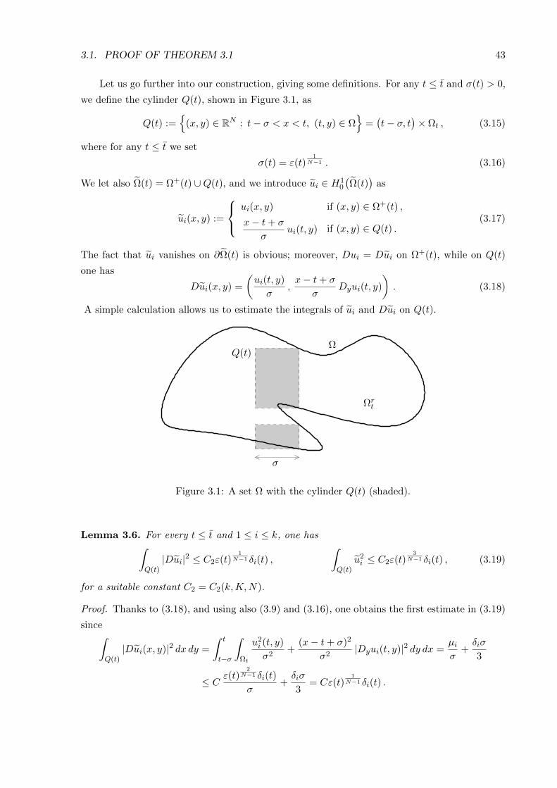
3.1. PROOF OF THEOREM 3.1 43
Let us go further into our construction, giving some definitions. For any t ≤ t and σ(t) > 0,
we define the cylinder Q(t), shown in Figure 3.1, as
Q(t) :=
(x, y) ∈ RN : t− σ < x < t, (t, y) ∈ Ω
=(t− σ, t
)× Ωt , (3.15)
where for any t ≤ t we set
σ(t) = ε(t)1
N−1 . (3.16)
We let also Ω(t) = Ω+(t) ∪Q(t), and we introduce ui ∈ H10
(Ω(t)
)as
ui(x, y) :=
ui(x, y) if (x, y) ∈ Ω+(t) ,
x− t+ σ
σui(t, y) if (x, y) ∈ Q(t) .
(3.17)
The fact that ui vanishes on ∂Ω(t) is obvious; moreover, Dui = Dui on Ω+(t), while on Q(t)
one has
Dui(x, y) =
(ui(t, y)
σ,x− t+ σ
σDyui(t, y)
). (3.18)
A simple calculation allows us to estimate the integrals of ui and Dui on Q(t).
Q(t)Ω
Ωrt
σ
Figure 3.1: A set Ω with the cylinder Q(t) (shaded).
Lemma 3.6. For every t ≤ t and 1 ≤ i ≤ k, one has∫Q(t)|Dui|2 ≤ C2ε(t)
1N−1 δi(t) ,
∫Q(t)
u2i ≤ C2ε(t)
3N−1 δi(t) , (3.19)
for a suitable constant C2 = C2(k,K,N).
Proof. Thanks to (3.18), and using also (3.9) and (3.16), one obtains the first estimate in (3.19)
since∫Q(t)|Dui(x, y)|2 dx dy =
∫ t
t−σ
∫Ωt
u2i (t, y)
σ2+
(x− t+ σ)2
σ2|Dyui(t, y)|2 dy dx =
µiσ
+δiσ
3
≤ C ε(t)2
N−1 δi(t)
σ+δiσ
3= Cε(t)
1N−1 δi(t) .
44 CHAPTER 3. EXISTENCE OF MINIMIZERS IN RN
On the other hand, the second estimate in (3.19) follows, also again using (3.9) and (3.16), by∫Q(t)
ui(x, y)2 dx dy =
∫ t
t−σ
∫Ωt
u2i (t, y) dy dx =
σµi3≤ Cσε(t)
2N−1 δi(t) = Cε(t)
3N−1 δi(t) .
Another simple but useful estimate concerns the Rayleigh quotients of the functions ui on
the sets Ω(t) and the integral of the products uiuj .
Lemma 3.7. For every t ≤ t and 1 ≤ i ≤ k, one has
R(ui, Ω(t)
)≤ λi(Ω) + Cε(t)
1N−1 δi(t) . (3.20)
Moreover, for every i 6= j ∈ 1, 2, . . . , k, one has∣∣∣∣ ∫Ω(t)
uiuj +Dui ·Duj∣∣∣∣ ≤ C(ε(t) 3
N−1 + ε(t)1
N−1
)√δi(t)δj(t) . (3.21)
Proof. Recalling that −∆ui = λi(Ω)ui, making use of (3.12) and (3.19) and arguing as in (3.13),
we obtain
R(ui, Ω(t)
)=
∫Ω+(t)
|Dui|2 +
∫Q(t)|Dui|2∫
Ω+(t)u2i +
∫Q(t)
u2i
≤
∫Ω+(t)
|Dui|2 +
∫Q(t)|Dui|2∫
Ω+(t)u2i
=
λi(Ω)
∫Ω+(t)
u2i +
∫Ωt
ui∂ui∂ν
+
∫Q(t)|Dui|2∫
Ω+(t)u2i
≤ λi(Ω) + Cε(t)1
N−1 δi(t) ,
hence (3.20) is proved.
On the other hand, recall that ui and uj are orthogonal on Ω both in L2 and in H10 sense
by definition, hence by using (3.10) and (3.19) we find∣∣∣∣ ∫Ω(t)
uiuj
∣∣∣∣ ≤ ∣∣∣∣ ∫Ω+(t)
uiuj
∣∣∣∣+
∣∣∣∣ ∫Q(t)
uiuj
∣∣∣∣ =
∣∣∣∣ ∫Ω−(t)
uiuj
∣∣∣∣+
∣∣∣∣ ∫Q(t)
uiuj
∣∣∣∣≤ C
(ε(t)
1N−1
√δi(t)δj(t) + ε(t)
3N−1
√δi(t)δj(t)
).
In the very same way, concerning Dui and Duj , we have∣∣∣∣ ∫Ω(t)
Dui ·Duj∣∣∣∣ ≤ ∣∣∣∣ ∫
Ω+(t)Dui ·Duj
∣∣∣∣+
∣∣∣∣ ∫Q(t)
Dui ·Duj∣∣∣∣
=
∣∣∣∣ ∫Ω−(t)
Dui ·Duj∣∣∣∣+
∣∣∣∣ ∫Q(t)
Dui ·Duj∣∣∣∣ ≤ Cε(t) 1
N−1
√δi(t)δj(t) .
Adding up the last two estimates yields (3.21).
3.1. PROOF OF THEOREM 3.1 45
In order to prove Lemma 3.4, we need to compare the eigenvalues of Ω and those of Ω(t);
this can be done by means of the min-max principle (2.4), which relates the eigenvalues with
the Rayleigh quotients of H10 functions.
Lemma 3.8. There exist a small constant ν = ν(k,K,N) < 1 and a constant C3 = C3(k,K,N)
such that, if ε(t), δi(t) ≤ ν for every 1 ≤ i ≤ k, then
λj(Ω(t)
)≤ λj(Ω) + C3ε(t)
1N−1 δ(t) ∀ 1 ≤ j ≤ k . (3.22)
Proof. We aim to use the characterization given by (2.4). To do so, for every 1 ≤ j ≤ k we
define Kj as the linear subspace of H10
(Ω(t)
)spanned by the functions ui with 1 ≤ i ≤ j. First
of all, we state and prove the following claim.
Claim 3.A.
For every 1 ≤ j ≤ k, the space Kj has dimension j.
Proof of Claim 3.A. Suppose that the claim is not true. Then, there should exist some 1 ≤ ` ≤ kand some coefficients βi for i 6= ` with all |βi| ≤ 1 and
u` =∑
1≤i≤k, i6=`βiui .
Notice now that by (3.12) we know that∫
Ω+(t) u2` ≥ 1/2, hence also by (3.21) we deduce
1
2≤∫
Ω(t)u2` =
∫Ω(t)
∑1≤i≤k, i6=`
βiuiu` ≤∑
1≤i≤k, i6=`
∣∣∣∣ ∫Ω(t)
uiu`
∣∣∣∣ ≤ k C(ν 3N−1 + ν
1N−1
)ν <
1
2,
where the last inequality is true provided that ν = ν(k,K,N) is chosen small enough. The
absurd shows the validity of Claim 3.A.
We can now show (3.22): to do so, pick a generic function w ∈ Kj , which can be written
(up to a rescaling) as w =∑j
i=1 βiui, where max|βi|, 1 ≤ i ≤ j
= 1. We need to evaluate
R(w, Ω(t)
): we start by noticing that
R(w, Ω(t)
)=
∫Ω(t)|Dw|2∫
Ω(t)w2
=
∑ji=1 β
2i
∫Ω(t)|Dui|2 +
∑i 6=j βiβj
∫Ω(t)
Dui ·Duj∑ji=1 β
2i
∫Ω(t)
u2i +
∑i 6=j βiβj
∫Ω(t)
uiuj
≤∑j
i=1 β2i
∫Ω(t)|Dui|2 + Ck2ε(t)
1N−1 δ(t)∑j
i=1 β2i
∫Ω(t)
u2i − Ck2ε(t)
1N−1 δ(t)
,
(3.23)
where the last inequality comes by (3.21). If ν(k,K,N) is small enough, then
Ck2ε(t)1
N−1 δ(t) ≤ Ck2νNN−1 ≤ 1
4,
hence by the choice of βi and by (3.12) the denominator in the last fraction of (3.23) is bigger
than 1/4 (in particular, it is strictly positive). As a consequence, recalling also that by (3.20)
46 CHAPTER 3. EXISTENCE OF MINIMIZERS IN RN
one has for every 1 ≤ i ≤ j∫Ω(t)|Dui|2∫
Ω(t)u2i
≤ λi(Ω) + Cε(t)1
N−1 δi(t) ≤ λj(Ω) + Cε(t)1
N−1 δ(t) ,
from (3.23) we deduce
R(w, Ω(t)
)≤
(λj(Ω) + Cε(t)
1N−1 δ(t)
)(∑ji=1 β
2i
∫Ω(t)
u2i
)+ Cε(t)
1N−1 δ(t)∑j
i=1 β2i
∫Ω(t)
u2i − Cε(t)
1N−1 δ(t)
≤
(λj(Ω) + Cε(t)
1N−1 δ(t)
)+ 2Cε(t)
1N−1 δ(t)
1− 2Cε(t)1
N−1 δ(t)≤ λj(Ω) + Cε(t)
1N−1 δ(t)
(keep in mind that the constant C = C(k,K,N) may increase from line to line). The validity
of (3.22) is then now an immediate consequence of (2.4) and of Claim 3.A.
We can now enter in the central part of our construction. Basically, we aim to show that
either Ω already satisfies the requirements of Lemma 3.4, or some Ω(t) does it, up to a rescaling.
To do so, we need another definition, namely, for every t ≤ t we define the rescaled set
Ω(t) :=∣∣Ω(t)
∣∣− 1N Ω(t) ,
so that∣∣Ω(t)
∣∣ = 1. We can now show the following result.
Lemma 3.9. Let Ω be as in the assumptions of Lemma 3.4, and let t ≤ t. There exists
C4 = C4(k,K,N) such that exactly one of the three following conditions hold:
(1) maxε(t), δ(t)
> ν;
(2) (1) does not hold and m(t) ≤ C4
(ε(t) + δ(t)
)ε(t)
1N−1 ;
(3) (1) and (2) do not hold and for every 1 ≤ i ≤ k, one has λi(Ω(t)
)< λi(Ω).
In particular, if condition (3) holds for t and m(t) ≥ m, then for every 1 ≤ i ≤ k one has
λi(Ω(t)
)< λi(Ω)− η, being η = η(k,K,N) > 0.
Proof. If (1) holds true, there is of course nothing to prove. Otherwise, it is possible to apply
Lemma 3.8, hence we have
λi(Ω(t)
)≤ λi(Ω) + C3ε(t)
1N−1 δ(t) (3.24)
for every 1 ≤ i ≤ k. By property (2) of Lemma 2.7 and the fact that∣∣Ω(t)
∣∣ = 1, we know that
λi(Ω(t)
)=∣∣Ω(t)
∣∣ 2N λi
(Ω(t)
).
3.1. PROOF OF THEOREM 3.1 47
By construction, ∣∣Ω(t)∣∣ =
∣∣Ω+(t)∣∣+∣∣Q(t)
∣∣ = 1−m(t) + ε(t)NN−1 ,
hence the above estimates and (3.24) lead to
λi(Ω(t)) =(
1−m(t) + ε(t)NN−1
) 2Nλi(Ω(t)
)≤(
1− 2
Nm(t) +
2
Nε(t)
NN−1
)(λi(Ω) + C3ε(t)
1N−1 δ(t)
)≤ λi(Ω)− 2λ1(BN )
Nm(t) +
2K
Nε(t)
NN−1 +
(C3 +
2
N
)ε(t)
1N−1 δ(t) .
(3.25)
This allows us to conclude. In fact, defining C4 := 2(K+1)N +C3, if m(t) ≤ C4
(ε(t)+δ(t)
)ε(t)
1N−1 ,
then condition (2) holds true. Otherwise, (3.25) directly implies that λi(Ω(t)
)< λi(Ω).
Finally, assume that condition (3) holds and m(t) ≥ m: in this case, (3.25) directly implies
λi(Ω(t)
)− λi(Ω) ≤ −2λ1(BN )
Nm+ C4ν
NN−1 ≤ −η ,
where η = λ1(BN )m/N and the last inequality is true up to decrease ν (notice that decreasing
the value of the constant ν of Lemma 3.8 does not change the value of C3).
We are finally in position to give the proof of Lemma 3.4.
Proof of Lemma 3.4. Let us start defining
t := supt ≤ t : condition (3) of Lemma 3.9 holds for t
, (3.26)
with the usual convention that, if condition (3) is false for every t ≤ t, then t = −∞. We
introduce now the following subsets of (t, t),
A : =t ∈ (t, t) : condition (1) of Lemma 3.9 holds for t
,
B : =t ∈ (t, t) : condition (2) of Lemma 3.9 holds for t and m(t) > 0
,
and we further subdivide them as
A1 :=t ∈ A : ε(t) ≥ δ(t)
, A2 :=
t ∈ A : ε(t) < δ(t)
,
B1 :=t ∈ B : ε(t) ≥ δ(t)
, B2 :=
t ∈ B : ε(t) < δ(t)
.
We aim to show that both A and B are uniformly bounded. Concerning A1, observe that
ν∣∣A1
∣∣ ≤ ∫A1
ε(t) dt =∣∣∣(x, y) ∈ Ω : x ∈ A1
∣∣∣ ≤ ∣∣Ω∣∣ = 1 ,
so that |A1| ≤ 1/ν. Concerning A2, in the same way and also recalling that λi(Ω) ≤ K for every
i ≤ k, we have
ν∣∣A2
∣∣ ≤ ∫A2
δ(t) dt =k∑i=1
∫A2
∫Ωt
∣∣Dui(t, y)∣∣2 dHN−1(y) dt ≤
k∑i=1
∫Ω
∣∣Dui∣∣2 ≤ kK ,
48 CHAPTER 3. EXISTENCE OF MINIMIZERS IN RN
so that |A2| ≤ kK/ν. Summarizing, we have proved that∣∣A∣∣ ≤ 1 + kK
ν. (3.27)
Let us then pass to the set B1. To deal with it, we need a further subdivision, namely, we write
B1 = ∪n∈NBn1 , where
Bn1 :=
t ∈ B1 :
m
2n< m(t) ≤ m
2n−1
. (3.28)
Keeping in mind (3.6), we know that t 7→ m(t) is an increasing function, and that for a.e. t ∈ Rone has m′(t) = ε(t). Moreover, for every t ∈ B1 one has by construction that
m(t) ≤ C4
(ε(t) + δ(t)
)ε(t)
1N−1 ≤ 2C4 ε(t)
NN−1 .
As a consequence, for every t ∈ Bn1 one has
m′(t) = ε(t) ≥ 1
Cm(t)
N−1N ≥ 1
Cm
N−1N
1(2N−1N
)n .This readily implies
1
Cm
N−1N
1(2N−1N
)n ∣∣Bn1
∣∣ ≤ ∫Bn1
m′(t) ≤ m
2n,
which in turn gives ∣∣Bn1
∣∣ ≤ Cm 1N(2−
1N)n.
Finally, we deduce
∣∣B1
∣∣ =∑n∈N
∣∣Bn1
∣∣ ≤ Cm 1N
∑n∈N
(2−
1N)n
= Cm1N
21N
21N − 1
. (3.29)
Notice that basically our argument consisted in using the fact that in B1 one has
m(t) ≤ Cε(t)NN−1 , with ε(t) = m′(t) . (3.30)
Concerning B2, we can almost repeat the same argument: in fact, thanks to (3.10), for every
t ∈ B2 we have
φ(t) =
k∑i=1
∫Ω−(t)
|Dui|2 ≤ C1 ε(t)1
N−1 δ(t) ≤ C1 δ(t)NN−1 , with δ(t) = φ′(t) .
which is the perfect analogous of (3.30) with δ and φ in place of ε and m respectively. Since as
already observed φ(t) ≤∑∫
Ω |Dui|2 ≤ kK, in analogy with (3.28) we can define
Bn2 :=
t ∈ B2 :
kK
2n+1< φ(t) ≤ kK
2n
,
thus the very same argument which lead to (3.29) now gives
∣∣B2
∣∣ =∑n∈N
∣∣Bn2
∣∣ ≤ C(kK) 1N∑n∈N
(2−
1N)n
= C(kK) 1N
21N
21N − 1
. (3.31)
3.1. PROOF OF THEOREM 3.1 49
Putting (3.27), (3.29) and (3.31) together, we find∣∣A∣∣+∣∣B∣∣ ≤ C5 = C5(k,K,N) . (3.32)
We will prove the validity of the lemma with the following choice of R1 and Γ1,
R1 = 2C5 + 4 , Γ1 = 2[K/η]+1 ,
where C5 = C5(k,K,N) and η = η(k,K,N) have been introduced in (3.32) and in Lemma 3.9
respectively. To obtain our proof, we will distinguish the possible cases for Ω.
Case I. One has t = −∞.
If this case happens, then condition (3) of Lemma 3.9 never holds true, i.e., for every t ≤ t
either condition (1) or (2) holds. Recalling the definition of A and B and (3.32), we deduce that
W (Ω, 0, m) ≤ C5. Therefore, the claim of Lemma 3.4 is immediately obtained simply taking
Ω = Ω, since R1 ≥ C5 and Γ1 ≥ 1.
Case II. One has t > −∞.
In this case, let us notice that it must be m(t) > 0, hence (t, t) ⊆ A ∪ B and thus by (3.32)
t ≥ t − C5. Let us now pick some t? ∈ [t − 1, t] for which condition (3) holds, and define
U1 := Ω(t?). By definition, U1 has unit volume, and λi(U1) < λi(Ω) for every 1 ≤ i ≤ k, being
condition (3) true for t?.
Observe now that by definition for every 2 ≤ p ≤ N one has πp(Ω(t?)
)= πp
(Ω+(t?)
), hence
diam(πp(U1)
)= diam
(πp(Ω(t?)
))= diam
(πp
(∣∣Ω(t?)∣∣− 1
N Ω(t?)))≤ 2 diam
(πp(Ω(t?)
))= 2 diam
(πp(Ω+(t?)
))≤ 2 diam
(πp(Ω)
),
where we have used that∣∣Ω(t?)
∣∣ ≥ 1/2. Concerning the widths of U1 and Ω, we can start
observing that
W(U1, m, 1
)=∣∣Ω(t?)
∣∣− 1N
(W(
Ω(t?), m∣∣Ω(t?)
∣∣, ∣∣Ω(t?)∣∣)) .
Moreover, since it is admissible to assume νNN−1 < m
2 and then∣∣Ω(t?)lt?∣∣ =
∣∣ε(t?) NN−1
∣∣ < ∣∣Ω(t?)∣∣m ,
we have
τ(
Ω(t?), m∣∣Ω(t?)
∣∣) = τ(
Ω, m∣∣Ω(t?)
∣∣+ 1−∣∣Ω(t?)
∣∣) ;
as a consequence, we evaluate
W(
Ω(t?), m∣∣Ω(t?)
∣∣, ∣∣Ω(t?)∣∣) = τ
(Ω(t?),
∣∣Ω(t?)∣∣)− τ(Ω(t?), m
∣∣Ω(t?)∣∣)
= τ(Ω, 1
)− τ(
Ω, m∣∣Ω(t?)
∣∣+ 1−∣∣Ω(t?)
∣∣) ≤ τ(Ω, 1)− τ(Ω, m)= W
(Ω, m, 1
),
50 CHAPTER 3. EXISTENCE OF MINIMIZERS IN RN
thus we deduce, again recalling∣∣Ω(t?)
∣∣ ≥ 1/2, that
W(U1, m, 1
)≤ 2W
(Ω, m, 1
).
Summarizing, we have found that
λi(U1) < λi(Ω) , diam(πp(U1)
)≤ 2 diam
(πp(Ω)
), W
(U1, m, 1
)≤ 2W
(Ω, m, 1
). (3.33)
As a consequence, the choice Ω = U1 satisfies all the requirements of Lemma 3.4, except possibly
condition (3.3). To deal with this last condition, we need to further subdivide this case.
Case IIa. One has t > −∞ and m(t?) < m.
In this case, we can show that the choice Ω = U1 actually works. As noticed above, we have
only to prove the validity of (3.3). To do so, we assume for simplicity that t = 0, which is clearly
admissible by translation. Hence, t? ≥ t− 1 ≥ t− C5 − 1 = −C5 − 1, and thus
Ω(t?) = Ω+(t?) ∪Q(t?) ⊆
(x, y) : x > t? − 1⊆
(x, y) : x > −C5 − 2.
Recalling that∣∣Ω(t?)
∣∣ ≥ ∣∣Ω+(t?)∣∣ ≥ |Ω+(t)| = 1− 2m ≥ 1/2, we deduce that
Ω = Ω(t?) =∣∣Ω(t?)
∣∣− 1N Ω(t?) ⊆ 2 Ω(t?) ⊆
(x, y) : x > −2C5 − 4
. (3.34)
Moreover, since m(t) < m,∣∣Ωl0
∣∣ =∣∣Ω(t?)l0
∣∣ ≥ ∣∣Ω(t?)l0∣∣ =
∣∣∣(Ω+(t?) ∪Q(t?))l
0
∣∣∣ ≥ ∣∣∣(Ω+(t?))l
0
∣∣∣=∣∣∣(x, y) ∈ Ω : t? < x < 0
∣∣∣ = m(0)−m(t?) ≥ m(0)−m(t) ≥ m ,
and this implies that τ(Ω, m) ≤ 0. The inclusion (3.34) ensures then that τ(Ω, 0) ≥ −2C5 − 4,
and then (3.3) holds true since R1 = 2C5 + 4.
Case IIb. One has t > −∞ and m(t?) ≥ m.
We have now to face the last possible case, namely, when t is finite but m(t?) ≥ m. In this case,
thanks to Lemma 3.9 the estimates (3.33) can be strengthened as
λi(U1) < λi(Ω)− η , diam(πp(U1)
)≤ 2 diam
(πp(Ω)
), W
(U1, m, 1
)≤ 2W
(Ω, m, 1
). (3.35)
Concerning the validity of (3.3), it does not follow by (3.34) because the assumption m(t) ≥ mdoes not imply that τ(Ω, m) ≤ 0. However, we can argue as follow: if (3.3) holds true for U1,
then of course we are done by setting Ω = U1. Otherwise, we apply the above construction to
the set U1 in place of Ω: since U1 does not satisfy (3.3), then Case I is impossible, thus we are
in Case II and then by (3.33) we find an open set U2 of unit measure such thatλi(U2) < λi(U1) < λi(Ω)− η ∀ 1 ≤ i ≤ k ,diam
(πp(U2)
)≤ 2 diam
(πp(U1)
)≤ 4 diam
(πp(Ω)
),
W(U2, m, 1
)≤ 2W
(U1, m, 1
)≤ 4W
(Ω, m, 1
).
3.1. PROOF OF THEOREM 3.1 51
If U1 is in Case IIa, then as before we are done with the choice of Ω = U2. Otherwise, if we are
in Case IIb, then (3.35) becomes
λi(U2) < λi(Ω)− 2η , diam(πp(U2)
)≤ 4 diam
(πp(Ω)
), W
(U2, m, 1
)≤ 4W
(Ω, m, 1
).
Going on with the obvious iteration, if the proof has not been concluded after ` ∈ N steps then
we have found an open set U` satisfying
λi(U`) < λi(Ω)− `η , diam(πp(U`)
)≤ 2` diam
(πp(Ω)
), W
(U`, m, 1
)≤ 2`W
(Ω, m, 1
).
This is of course impossible if `η ≥ K, being λk(Ω) ≤ K: as a consequence, our iteration must
stop after less than K/η steps, thus our thesis is concluded with our choice of Γ1.
3.1.2 Boundedness of the interior
The goal of this subsection is to obtain a uniform bound also for the interior part of a set Ω, in
the sense of Lemma 3.4. Most of the arguments of this case will be identical to those that we
made for the tails in Section 3.1.1, but some modifications are essential. In particular we give
new definitions for ε, δi, µi, Ω(t) and Ω(t) in order to maintain the analogy with what was done
in Section 3.1.1. The result that we are going to prove is the following.
Lemma 3.10. For every K > 0 there exist R2 = R2(k,K,N) and Γ2 = Γ2(k,K,N) such that,
for any open set Ω ⊆ RN of unit volume and with λk(Ω) ≤ K, and for any choice of m ∈(m, 1− m
2 ), there exists another open set Ω ⊆ RN , still of unit volume, such that λi(Ω) ≤ λi(Ω)
for every 1 ≤ i ≤ k, and such that for every 2 ≤ p ≤ N
W(Ω, 0,m
)≤ R2 + Γ2W
(Ω, 0,m− m
), diam
(πp(Ω)
)≤ Γ2 diam
(πp(Ω)
). (3.36)
To start with, we give the analogous of the definitions (3.5), (3.6) and (3.7) of Section 3.1.1
that we need now; Figure 3.2 helps to visualize the new situation. More precisely, we set for
brevity
t0 :=τ(Ω,m+ m
2 ) + τ(Ω,m− m)
2, t :=
τ(Ω,m+ m2 )− τ(Ω,m− m)
2;
keep in mind that, since m ∈ (m, 1− m2 ), then −∞ < τ(Ω,m− m) < τ(Ω,m+ m
2 ) < +∞. For
any 0 ≤ t ≤ t, we define
Ω+(t) := Ωlt0−t ∪ Ωr
t0+t , Ω−(t) := Ωrt0−t ∩ Ωl
t0+t = Ω \ Ω+(t) ,
ε(t) := HN−1(Ωt0−t) +HN−1(Ωt0+t) , m(t) :=∣∣Ω−(t)
∣∣ =
∫ t
0ε(s) ds ≤ 3
2m .
Moreover, having fixed an orthonormal setu1, u2, . . . , uk
of eigenfunctions with unit L2
norm corresponding to the first k eigenvalues of Ω, for every 1 ≤ i ≤ k and 0 ≤ t ≤ t we define
δi(t) :=
∫Ωt0−t
|Dui|2 +
∫Ωt0+t
|Dui|2 , µi(t) :=
∫Ωt0−t
u2i +
∫Ωt0+t
u2i .
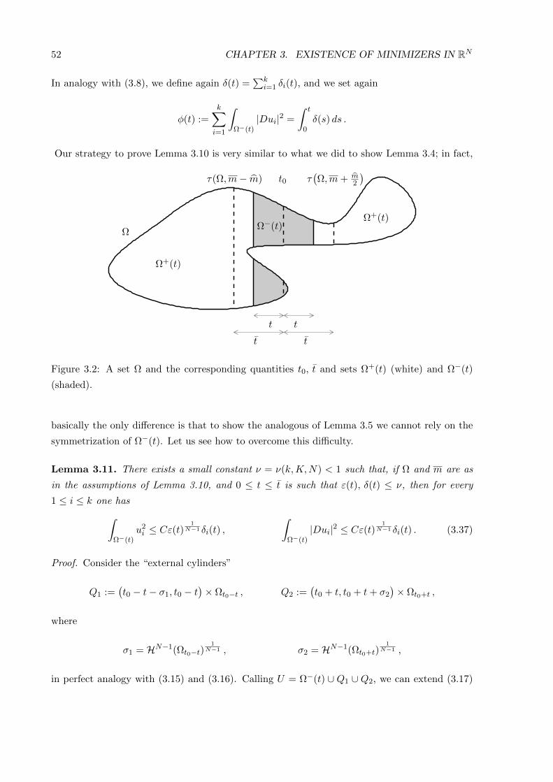
52 CHAPTER 3. EXISTENCE OF MINIMIZERS IN RN
In analogy with (3.8), we define again δ(t) =∑k
i=1 δi(t), and we set again
φ(t) :=
k∑i=1
∫Ω−(t)
|Dui|2 =
∫ t
0δ(s) ds .
Our strategy to prove Lemma 3.10 is very similar to what we did to show Lemma 3.4; in fact,
Ω−(t)Ω
Ω+(t)
Ω+(t)
t t
t0
t t
τ(Ω,m− m) τ(Ω,m+ m
2
)
Figure 3.2: A set Ω and the corresponding quantities t0, t and sets Ω+(t) (white) and Ω−(t)
(shaded).
basically the only difference is that to show the analogous of Lemma 3.5 we cannot rely on the
symmetrization of Ω−(t). Let us see how to overcome this difficulty.
Lemma 3.11. There exists a small constant ν = ν(k,K,N) < 1 such that, if Ω and m are as
in the assumptions of Lemma 3.10, and 0 ≤ t ≤ t is such that ε(t), δ(t) ≤ ν, then for every
1 ≤ i ≤ k one has∫Ω−(t)
u2i ≤ Cε(t)
1N−1 δi(t) ,
∫Ω−(t)
|Dui|2 ≤ Cε(t)1
N−1 δi(t) . (3.37)
Proof. Consider the “external cylinders”
Q1 :=(t0 − t− σ1, t0 − t
)× Ωt0−t , Q2 :=
(t0 + t, t0 + t+ σ2
)× Ωt0+t ,
where
σ1 = HN−1(Ωt0−t)1
N−1 , σ2 = HN−1(Ωt0+t)1
N−1 ,
in perfect analogy with (3.15) and (3.16). Calling U = Ω−(t) ∪ Q1 ∪ Q2, we can extend (3.17)
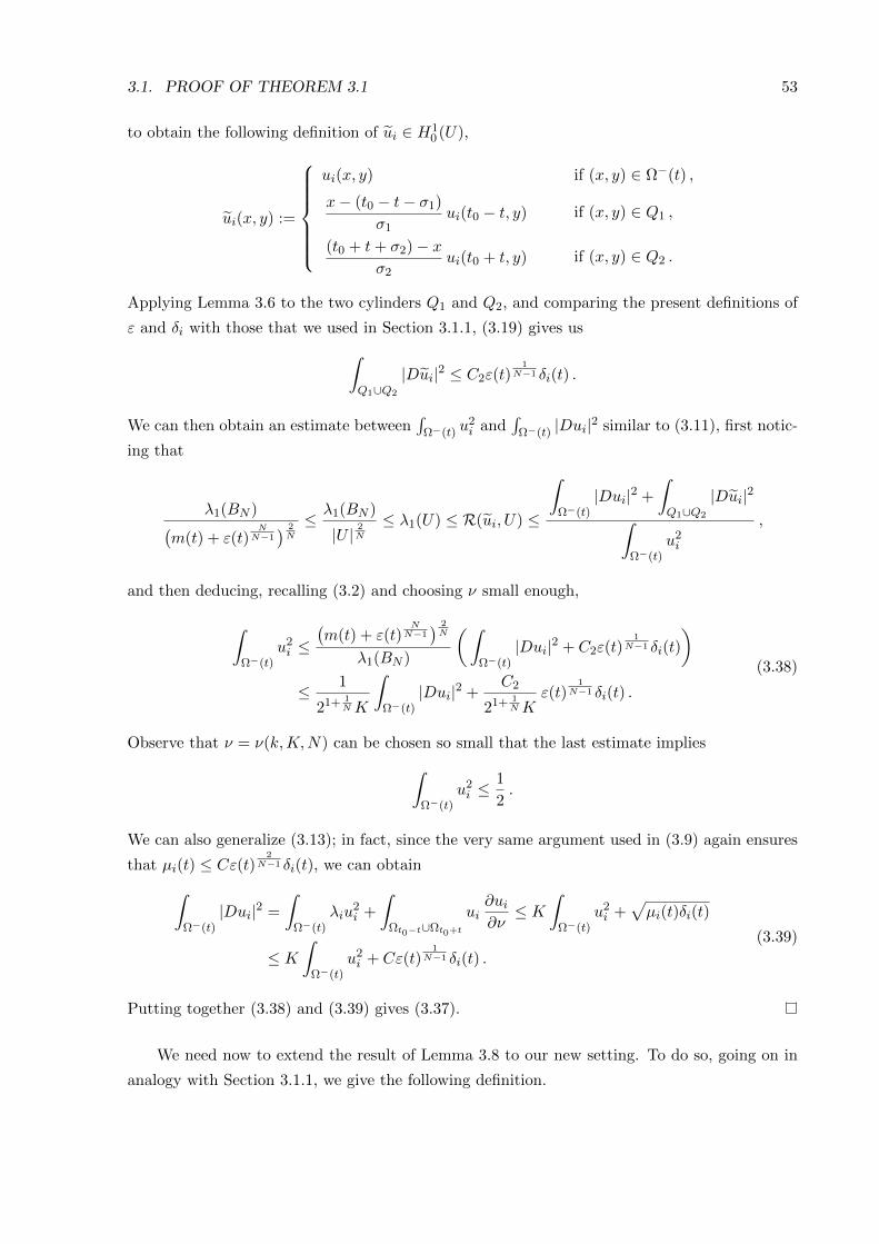
3.1. PROOF OF THEOREM 3.1 53
to obtain the following definition of ui ∈ H10 (U),
ui(x, y) :=
ui(x, y) if (x, y) ∈ Ω−(t) ,
x− (t0 − t− σ1)
σ1ui(t0 − t, y) if (x, y) ∈ Q1 ,
(t0 + t+ σ2)− xσ2
ui(t0 + t, y) if (x, y) ∈ Q2 .
Applying Lemma 3.6 to the two cylinders Q1 and Q2, and comparing the present definitions of
ε and δi with those that we used in Section 3.1.1, (3.19) gives us∫Q1∪Q2
|Dui|2 ≤ C2ε(t)1
N−1 δi(t) .
We can then obtain an estimate between∫
Ω−(t) u2i and
∫Ω−(t) |Dui|
2 similar to (3.11), first notic-
ing that
λ1(BN )(m(t) + ε(t)
NN−1
) 2N
≤ λ1(BN )
|U |2N
≤ λ1(U) ≤ R(ui, U) ≤
∫Ω−(t)
|Dui|2 +
∫Q1∪Q2
|Dui|2∫Ω−(t)
u2i
,
and then deducing, recalling (3.2) and choosing ν small enough,
∫Ω−(t)
u2i ≤
(m(t) + ε(t)
NN−1
) 2N
λ1(BN )
(∫Ω−(t)
|Dui|2 + C2ε(t)1
N−1 δi(t)
)≤ 1
21+ 1NK
∫Ω−(t)
|Dui|2 +C2
21+ 1NK
ε(t)1
N−1 δi(t) .
(3.38)
Observe that ν = ν(k,K,N) can be chosen so small that the last estimate implies∫Ω−(t)
u2i ≤
1
2.
We can also generalize (3.13); in fact, since the very same argument used in (3.9) again ensures
that µi(t) ≤ Cε(t)2
N−1 δi(t), we can obtain∫Ω−(t)
|Dui|2 =
∫Ω−(t)
λiu2i +
∫Ωt0−t∪Ωt0+t
ui∂ui∂ν≤ K
∫Ω−(t)
u2i +
√µi(t)δi(t)
≤ K∫
Ω−(t)u2i + Cε(t)
1N−1 δi(t) .
(3.39)
Putting together (3.38) and (3.39) gives (3.37).
We need now to extend the result of Lemma 3.8 to our new setting. To do so, going on in
analogy with Section 3.1.1, we give the following definition.
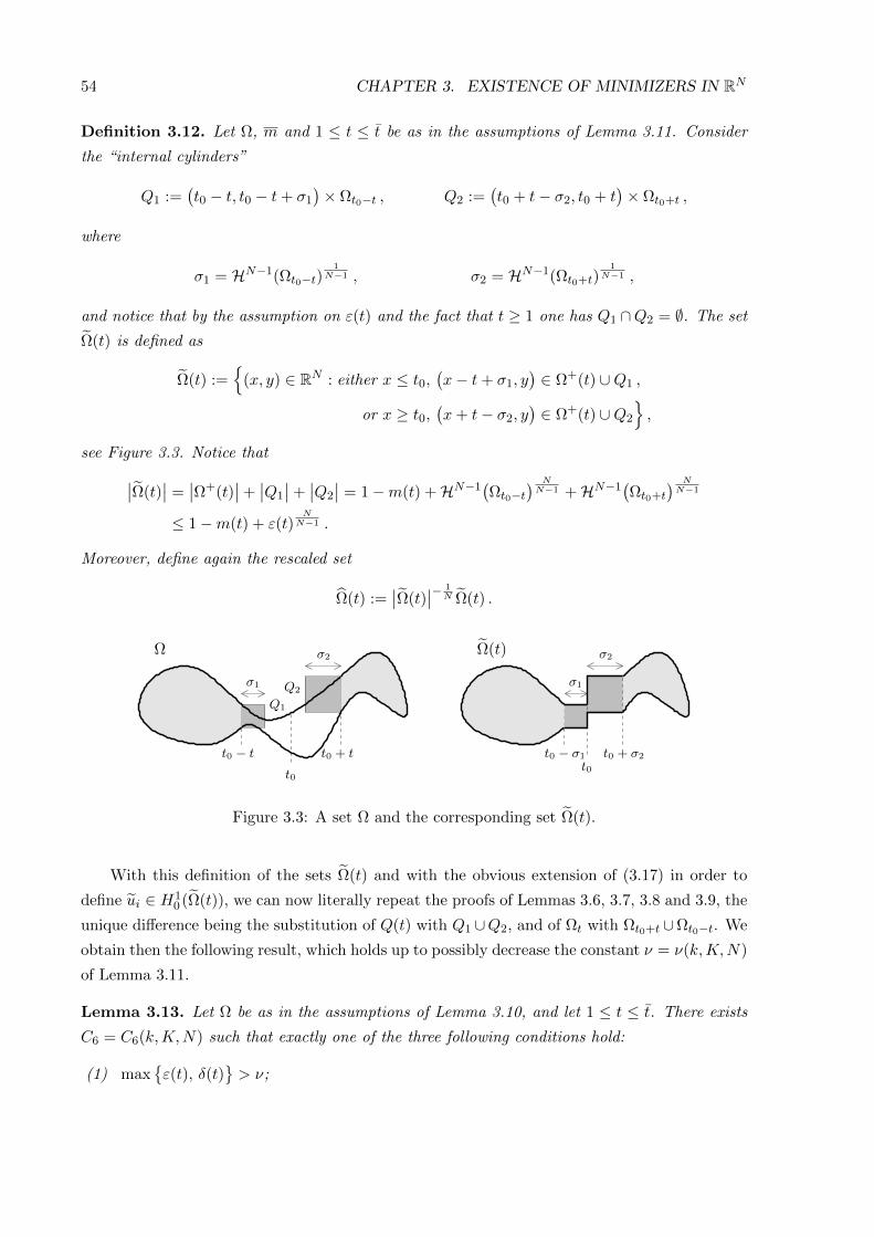
54 CHAPTER 3. EXISTENCE OF MINIMIZERS IN RN
Definition 3.12. Let Ω, m and 1 ≤ t ≤ t be as in the assumptions of Lemma 3.11. Consider
the “internal cylinders”
Q1 :=(t0 − t, t0 − t+ σ1
)× Ωt0−t , Q2 :=
(t0 + t− σ2, t0 + t
)× Ωt0+t ,
where
σ1 = HN−1(Ωt0−t)1
N−1 , σ2 = HN−1(Ωt0+t)1
N−1 ,
and notice that by the assumption on ε(t) and the fact that t ≥ 1 one has Q1 ∩Q2 = ∅. The set
Ω(t) is defined as
Ω(t) :=
(x, y) ∈ RN : either x ≤ t0,(x− t+ σ1, y
)∈ Ω+(t) ∪Q1 ,
or x ≥ t0,(x+ t− σ2, y
)∈ Ω+(t) ∪Q2
,
see Figure 3.3. Notice that∣∣Ω(t)∣∣ =
∣∣Ω+(t)∣∣+∣∣Q1
∣∣+∣∣Q2
∣∣ = 1−m(t) +HN−1(Ωt0−t
) NN−1 +HN−1
(Ωt0+t
) NN−1
≤ 1−m(t) + ε(t)NN−1 .
Moreover, define again the rescaled set
Ω(t) :=∣∣Ω(t)
∣∣− 1N Ω(t) .
t0 − t t0 + t
σ2
Q2
Q1
Ω(t)
t0 − σ1
σ2
t0 + σ2
σ1σ1
t0t0
Ω
Figure 3.3: A set Ω and the corresponding set Ω(t).
With this definition of the sets Ω(t) and with the obvious extension of (3.17) in order to
define ui ∈ H10 (Ω(t)), we can now literally repeat the proofs of Lemmas 3.6, 3.7, 3.8 and 3.9, the
unique difference being the substitution of Q(t) with Q1 ∪Q2, and of Ωt with Ωt0+t ∪Ωt0−t. We
obtain then the following result, which holds up to possibly decrease the constant ν = ν(k,K,N)
of Lemma 3.11.
Lemma 3.13. Let Ω be as in the assumptions of Lemma 3.10, and let 1 ≤ t ≤ t. There exists
C6 = C6(k,K,N) such that exactly one of the three following conditions hold:
(1) maxε(t), δ(t)
> ν;
3.1. PROOF OF THEOREM 3.1 55
(2) (1) does not hold and m(t) ≤ C6
(ε(t) + δ(t)
)ε(t)
1N−1 ;
(3) (1) and (2) do not hold and for every 1 ≤ i ≤ k, one has λi(Ω(t)
)< λi(Ω).
In particular, if condition (3) holds for t and m(t) ≥ m/2, then for every 1 ≤ i ≤ k one has
λi(Ω(t)
)< λi(Ω)− η, being η = η(k,K,N) > 0.
We can now conclude this section by presenting the proof of Lemma 3.10, which will be a
minor modification of the proof of Lemma 3.4.
Proof of Lemma 3.10. First of all, we want to show that it is admissible to assume
m(t) > 0 ∀ t > 0 . (3.40)
In fact, suppose that it is not so, and let τ = max0 ≤ t ≤ t : m(t) = 0 > 0. Then, Ω is
the disjoint union of Ω ∩ x > t0 + τ and Ω ∩ x < t0 − τ, and it does not intersect the
whole strip t0 − τ < x < t0 + τ. Therefore, replacing Ω with
(x + τ, y) : x < t0, (x, y) ∈Ω∪
(x − τ, y) : x > t0, (x, y) ∈ Ω
, that is, moving closer the two disjoint parts of Ω, does
not change any of the eigenvalues of Ω and is clearly admissible for the proof of the lemma;
moreover, the property (3.40) of course holds true for this new set. Hence, from now on we
directly assume that (3.40) holds true for Ω.
Define now t analogously to (3.26) by setting
t := sup
1 ≤ t ≤ t : condition (3) of Lemma 3.13 holds for t,
with the convention that, if condition (3) is false for every 1 ≤ t ≤ t, then t = 1. Again we
define A and B as
A : =t ∈ (t, t) : condition (1) of Lemma 3.13 holds for t
,
B : =t ∈ (t, t) : condition (2) of Lemma 3.13 holds for t and m(t) > 0
.
The same argument of the proof of Lemma 3.4 gives then∣∣A∣∣+∣∣B∣∣ ≤ C7 = C7(k,K,N) , (3.41)
and we are going to show the thesis with the choice
R2 = 4C7 + 8 , Γ2 = 2[K/η]+1 ,
being η the constant of Lemma 3.13. We can again subdivide the possible cases for Ω.
Case I. One has t = 1.
In this case, by (3.40) one has that every 1 < t ≤ t belongs either to A or to B, thus by (3.41)
56 CHAPTER 3. EXISTENCE OF MINIMIZERS IN RN
t ≤ C7 + 1; as a consequence, the choice Ω = Ω satisfies the requirements of the lemma. Indeed,
while the right condition of (3.36) is obviously true, the left one follows just noticing that
W(Ω, 0,m
)= W
(Ω, 0,m
)= τ(Ω,m)− τ(Ω,m− m) +W
(Ω, 0,m− m
)≤ τ
(Ω,m+
m
2
)− τ(Ω,m− m) +W
(Ω, 0,m− m
)= 2t+W
(Ω, 0,m− m
)≤ 2(C7 + 1
)+W
(Ω, 0,m− m
).
Case II. One has t > 1.
In this case, again by (3.40) we know that A∪B contains the whole segment (t, t), thus t ≤ t+C7
by (3.41). If we choose t? ∈ (t − 1, t) for which condition (3) holds and define U1 := Ω(t?), we
know by construction that |U1| = 1 and λi(U1) < λi(Ω) for every 1 ≤ i ≤ k. As in the proof of
Lemma 3.4, the fact that |Ω(t?)| ≥ 1 − 32m ≥ 1/2 ensures that diam
(πp(U1)
)≤ 2 diam
(πp(Ω)
)for each 2 ≤ p ≤ N . On the other hand, concerning the width of U1, recalling the definition of
Ω(t?) and observing that (m− m)∣∣Ω(t?)
∣∣ < m− m one finds
W(U1, 0,m− m
)= W
(Ω(t?), 0,m− m
)=∣∣Ω(t?)
∣∣− 1NW
(Ω(t?), 0, (m− m)
∣∣Ω(t?)∣∣)
≤ 2
(τ(
Ω(t?), (m− m)∣∣Ω(t?)
∣∣)− τ(Ω(t?), 0))
= 2
(τ(
Ω, (m− m)∣∣Ω(t?)
∣∣)− τ(Ω, 0))
= 2W(
Ω, 0, (m− m)∣∣Ω(t?)
∣∣)≤ 2W
(Ω, 0,m− m
).
Summarizing, we have found that
λi(U1) < λi(Ω) ,diam
(πp(U1)
)diam
(πp(Ω)
) ≤ 2 ,W(U1, 0,m− m
)W(Ω, 0,m− m
) ≤ 2 . (3.42)
To conclude the inspection of the validity of (3.36), we will again need to consider separately
two subcases.
Case IIa. One has t > 1 and m(t?) ≤ m/2.
In this case, we can quickly observe that
W(U1, 0,m
)=∣∣Ω(t?)
∣∣− 1NW
(Ω(t?), 0,m
∣∣Ω(t?)∣∣) ≤ 2W
(Ω(t?), 0,m+
m
2−∣∣Ω−(t?)
∣∣)≤ 2W
(Ω, 0,m− m
)+ 4(t− t? + 1
)≤ 2W
(Ω, 0,m− m
)+ 4(C7 + 2
),
(3.43)
and, together with (3.42), this concludes the proof of (3.36) and of the lemma with the choice
Ω = U1.
Case IIb. One has t > 1 and m(t?) > m/2.
Let us conclude with this last case. By Lemma 3.13, in place of (3.42) we have then
λi(U1) < λi(Ω)− η ,diam
(πp(U1)
)diam
(πp(Ω)
) ≤ 2 ,W(U1, 0,m− m
)W(Ω, 0,m− m
) ≤ 2 ,
3.1. PROOF OF THEOREM 3.1 57
which still does not guarantee the validity of (3.36). However, we can apply the construction
above to U1: if U1 is in Case I, then the choice Ω = U1 concludes the proof; otherwise, there
exists an open set U2 of unit measure satisfying
λi(U2) < λi(Ω)− η ,diam
(πp(U2)
)diam
(πp(Ω)
) ≤ 4 ,W(U2, 0,m− m
)W(Ω, 0,m− m
) ≤ 4 . (3.44)
If U1 is in Case IIa then (3.43) gives
W(U2, 0,m
)≤ 2W
(U1, 0,m− m
)+ 4(C7 + 2
)≤ 4W
(Ω, 0,m− m
)+ 4(C7 + 2
),
so the choice Ω = U2 concludes the proof. Instead, if U1 is in Case IIb then the first inequality
of (3.44) becomes λi(U2) < λi(Ω) − 2η for every 1 ≤ i ≤ k. The obvious iteration ensures us
that, if the proof has not been obtained after ` steps, then there must be some open set U`
satisfying
λi(U`) < λi(Ω)− `η ,diam
(πp(U`)
)diam
(πp(Ω)
) ≤ 2` ,W(U`, 0,m− m
)W(Ω, 0,m− m
) ≤ 2` .
Since this is not possible for ` > K/η, the iteration must stop at some ` ≤ [K/η], and thus we
conclude the proof thanks to the choice of Γ2.
3.1.3 Proof of Proposition 3.2
We are finally in position to give the proof of Proposition 3.2, which is now a simple consequence
of Lemma 3.4 and Lemma 3.10.
Proof of Proposition 3.2. Let us pick a generic open set Ω with λk(Ω) ≤ K. Applying Lemma 3.4
to Ω, we find a set E1 with
λi(E1) ≤ λi(Ω) , W (E1, 0, m) ≤ R1 ,diam
(πp(E1)
)diam
(πp(Ω)
) ≤ Γ1 ,
for every 2 ≤ p ≤ N . Then, we apply Lemma 3.10 to E1 with m = 2m finding E2 which satisfies
λi(E2) ≤ λi(Ω) , W (E2, 0, 2m) ≤ R2 + Γ2R1 ,diam
(πp(E2)
)diam
(πp(Ω)
) ≤ Γ2Γ1 .
Iterating, for any ` ≥ 3 such that `m ≤ 1 − m2 we apply Lemma 3.10 to E`−1 with m = `m
finding E` such that
λi(E`) ≤ λi(Ω) , W (E`, 0, `m) ≤ R2Γ`−1
2 − 1
Γ2 − 1+ Γ`−1
2 R1 ,diam
(πp(E`)
)diam
(πp(Ω)
) ≤ Γ`−12 Γ1 .
Possibly applying a last time Lemma 3.10 with m = 1− m, we have then found an open set E
satisfying
λi(E) ≤ λi(Ω) , W (E, 0, 1− m) ≤ R2Γ
[1/m]−12 − 1
Γ2 − 1+ Γ
[1/m]−12 R1,
diam(πp(E)
)diam
(πp(Ω)
) ≤ Γ[1/m]−12 Γ1.
58 CHAPTER 3. EXISTENCE OF MINIMIZERS IN RN
Calling E′ the set obtained by reflecting E with respect to the plane x = 0, the above estimates
become
λi(E′) ≤ λi(Ω) , W (E′, m, 1) ≤ R2
Γ[1/m]−12 − 1
Γ2 − 1+ Γ
[1/m]−12 R1 ,
diam(πp(E
′))
diam(πp(Ω)
) ≤ Γ[1/m]−12 Γ1 ,
so that applying once again Lemma 3.4 to E′ we find a set F1 satisfying
λi(F1) ≤ λi(Ω) , diam(π1(F1)
)= W (F1, 0, 1) ≤ R3 ,
diam(πp(F1)
)diam
(πp(Ω)
) ≤ Γ3 ,
having set
R3 := R1 + Γ1R2Γ
[1/m]−12 − 1
Γ2 − 1+ Γ1Γ
[1/m]−12 R1 , Γ3 := Γ
[1/m]−12 Γ2
1 .
We can now repeat the whole construction, using as starting set F1 in place of Ω, and using the
second coordinate in place of the first one. We will end up with a set F2 with
λi(F2) ≤ λi(F1) ≤ λi(Ω) ∀ 1 ≤ i ≤ k , diam(π2(F2)
)≤ R3 ,
and such that for every p 6= 2 it is diam(πp(F2)
)≤ Γ3 diam
(πp(F1)
). In particular, choosing
p = 1 we discover that diam(π1(F2)
)≤ Γ3R3. We have now to iterate also this argument:
for any 3 ≤ j ≤ N we repeat the above construction starting from Fj−1 and using the j-th
coordinate in the whole procedure, obtaining a set Fj which satisfies
λi(Fj)≤ λi(Ω) ∀1 ≤ i ≤ k , diam
(πp(Fj)
)≤ Γj−p3 R3 ∀ 1 ≤ p ≤ j .
The thesis is then finally obtained by defining Ω := FN , being R := ΓN−13 R3.
3.2 Boundedness of all minimizers
With a small improvement in the proof of Theorem 3.1, it is possible to prove that all the
minimizers for problem (3.1) have diameter uniformly bounded by a constant depending only
on k,N , if the functional F is weakly strictly increasing. Without this further assumption also
a constant functional would be admissible and in that case the uniform boundedness of all
minimizers is clearly false. The results of this section come from [M3].
Definition 3.14. A functional F : Rk → R is said to be weakly strictly increasing if for every
(x1, . . . , xN ), (y1, . . . , yk) ∈ Rk with xi > yi for all i = 1, . . . , k we have
F (x1, . . . , xk) > F (y1, . . . , yk).
We now state the Theorem and then we pass to its prove. As in the previous section we
first study the “tails”, then the interior and at the end we put all the informations together.
3.2. BOUNDEDNESS OF ALL MINIMIZERS 59
Theorem 3.15. Let k,N ∈ N and F : Rk → R be weakly strictly increasing and l.s.c.. Then
every minimizer for problem (3.1) is contained (up to translations) in an N -cube QR, where
R = R(k,N).
The idea of the proof is to show that, given a minimizer Ω∗ for (3.1) and a sequence of open
sets (Ωn)n∈N which γ-converges to Ω∗, then either Ωn are uniformly bounded (and so it is Ω∗)
or it is possible to find another minimizing sequence that contradicts the minimality of Ω∗.
During all the proof we will use the same notation of Section 3.1.
3.2.1 “Tails”
Throughout all this subsection and the next one, Ω ⊂ RN is an open set of unit volume such
that λk(Ω) ≤ K. We will choose K := Mλk(BN ), where M is the constant from Theorem 2.12,
so this big constant actually depends only on k,N . We also remind that the constant m(k,N)
is taken as in (3.2). We begin by proving a slightly stronger version of Lemma 3.8.
Lemma 3.16. Let Ω be an open set of unit volume, with λk(Ω) ≤ K. There exist a constant
C3 = C3(k,N) such that, if t ≤ t, then
λj(Ω(t)) ≤ λj(Ω) + C3
(ε(t)
NN−1 + δ(t)
NN−1
)∀1 ≤ j ≤ k.
Proof. It is clear that, thanks to Lemma 3.8, whenever ε(t), δi(t) ≤ ν for all i = 1, . . . , k, then
the thesis is true with C3 = C3, since ε(t)1
N−1 δ(t) ≤ ε(t)NN−1 + δ(t)
NN−1 .
We can now focus on the case when either ε(t) > ν or δi(t) > ν for some i. Then, we remind
that, since the first eigenfunction has not orthogonality constraints, Lemma 3.7 assures:
λ1(Ω(t)) ≤ λ1(Ω) + Cε(t)1
N−1 δi(t).
Thanks to Theorem 2.12 there exists a constant M > 0 such that λk(Ω)λ1(Ω) ≤ M for all Ω ⊂ RN .
Hence we can write, for all 1 ≤ j ≤ k:
λj(Ω(t)) ≤Mλ1(Ω(t)) ≤M(λ1(Ω) + Cε(t)
1N−1 δ(t)
).
Moreover it is possible to find a big constant A = A(k,N), such that MK ≤ AνNN−1 and then,
defining C3 = A+MC, we can conclude the computations above:
λj(Ω(t)) ≤M(K + Cε(t)
1N−1 δ(t)
)≤ Aν
NN−1 +MCε(t)
1N−1 δ(t)
≤ λj(Ω) +AνNN−1 +MCε(t)
1N−1 δ(t) ≤ λj(Ω) + C3
(ε(t)
NN−1 + δ(t)
NN−1
).
We are now in position to state and prove the main Lemma of this section.
Lemma 3.17. Let Ω be an open set of unit volume, with λk(Ω) ≤ K and t ≤ t. Then there
exists a constant C4 = C4(k,N) such that exactly one of the following situations happens.
60 CHAPTER 3. EXISTENCE OF MINIMIZERS IN RN
(1) m(t) ≤ C4
(ε(t)
NN−1 + δ(t)
NN−1
).
(2) (1) does not hold and for all 1 ≤ i ≤ k, λi(Ω(t)) < λi(Ω). Moreover for every m > 0 such
that m(t) ≥ m, there exists an η = η(N, m) such that for all 1 ≤ i ≤ k,
λi(Ω(t)) < λi(Ω)− η.
Proof. From Lemma 3.16 we have
λi(Ω(t)) ≤ λi(Ω) + C3
(ε(t)
NN−1 + δ(t)
NN−1
)∀1 ≤ i ≤ k,
moreover, putting in account that |Ω(t)| = |Ω+(t)|+ |Q(t)| = 1−m(t) + ε(t)NN−1 and the scaling
of the eigenvalues, then for all 1 ≤ i ≤ k
λi(Ω(t)) ≤(
1−m(t) + ε(t)NN−1
) 2N(λi(Ω) + C3
(ε(t)
NN−1 + δ(t)
NN−1
))≤ λi(Ω)− 2
Nλ1(BN )m(t) +
2K
Nε(t)
NN−1 + C3
(ε(t)
NN−1 + δ(t)
NN−1
)− 2
Nm(t)C3
(ε(t)
NN−1 + δ(t)
NN−1
)+
2
NC3ε(t)
NN−1
(ε(t)
NN−1 + δ(t)
NN−1
).
(3.45)
Then if m(t) ≤ C4
(ε(t)
NN−1 + δ(t)
NN−1
), condition (1) holds true; otherwise
m(t) > C4
(ε(t)
NN−1 + δ(t)
NN−1
),
and we can choose C4 ≥ 1 so that m(t) ≥ ε(t)NN−1 . Thus from the two last terms of (3.45), we
have
− 2
Nm(t)C3
(ε(t)
NN−1 + δ(t)
NN−1
)+
2
NC3ε(t)
NN−1
(ε(t)
NN−1 + δ(t)
NN−1
)≤ 0.
This allows us to conclude, choosing C4 ≥ 2K+NC3λ1(BN ) and obtaining:
λi(Ω(t))− λi(Ω) ≤ −λ1(BN )
Nm(t) < 0,
that is condition (2). Moreover if m(t) ≥ m, then we can improve the above estimate:
λi(Ω(t))− λi(Ω) ≤ −λ1(BN )
Nm = −η(N, m) < 0,
and the proof is concluded.
We introduce the following notations. Given an open set Ω as in the hypotheses of Lemma
3.17, we set
t = supt ∈ (−∞, t) : condition (2) of Lemma 3.17 holds for t
, (3.46)
with the usual convention that t = −∞ if condition (2) is false for every t ≤ t. If t > −∞, then
m(t) > 0 and we choose some t? ∈ [t− 1, t] for which condition (2) holds. The following Lemma
concludes this Section.
3.2. BOUNDEDNESS OF ALL MINIMIZERS 61
Lemma 3.18. Let (Ωn)n be as in the hypotheses of Lemma 3.17 and Ωnγ→ Ω.
(a) If there exists a subsequence (not relabeled) such that, for all n, m(t?(n)) ≥ m > 0 for
some m > 0, then Ω is not optimal for problem (3.1).
(b) If there exists a subsequence such that t(n) = −∞ for all n, then there exists R1 =
R1(k,N) > 0 such that W (Ω, 0, m) ≤ R1.
(c) If there exists a subsequence such that m(t?(n)) → 0 as n → ∞, then we have again
W (Ω, 0, m) ≤ R1.
Proof. We introduce the following subsets of (t(n), t(n)) for all n ∈ N:
An1 = t ∈ (t(n), t(n)) : ε(t) ≥ δ(t), An2 = t ∈ (t(n), t(n)) : ε(t) < δ(t).
Then, using Lemma 3.17, it is clear that for all t ∈ An1 , m(t) ≤ 2C4ε(t)NN−1 , while for all t ∈ An2 ,
thanks to Lemma 3.6 and reminding (3.8), φ(t) ≤ 2C1δ(t)NN−1 . Hence, since ε(t) = m′(t) and
δ(t) = φ′(t), we can work as in the proof of Lemma 3.4 and deduce that |An1 ∪ An2 | ≤ C5 =
C5(k,N).
If we are in case (b), since t(n) = −∞ for all n, then W (Ωn, 0, m) ≤ |An1 ∪ An2 | ≤ C5 and
the same is true for the γ-limit Ω.
On the other hand, if case (c) happens, in principle there could be some pieces of the limit
Ω outside the bounded strip, but it is clear from property (3) of Lemma 2.5 that Ω must have
zero capacity and not only zero Lebesgue measure outside the bounded strip. More precisely,
we can choose (up to translations) the origin such that m(0) = m. Since Ω corresponds to a
capacitary measure µΩ (see (2.3)), from point (c) we have that
µΩ ≡ ∞ in
(x, y) ∈ R× RN−1 : x < −C5
.
Hence W (Ω, 0, m) ≤ C5.
At last we consider case (a). Thanks to Lemma 3.17, we have that for all n and for all
1 ≤ i ≤ k,
λi(Ω(t?(n))) < λi(Ω)− η.
Hence, since we are supposing F to be weakly strictly increasing, we have a sequence (Ω(t?(n)))n
such that
infnF(λ1(Ω(t?(n))), . . . , λk(Ω(t?(n)))
)< F (λ1(Ω), . . . , λk(Ω)),
thus Ω can not be optimal for (3.1).
Remark 3.19. Applying Lemma 3.18 to a sequence of open sets (Ωn)n∈N satisfying the hypothe-
ses of Lemma 3.17 and which γ-converges to Ω∗, since (a), (b) and (c) cover all the possible
situations, we deduce
W (Ω∗, 0, m) ≤ R1(k,N).
62 CHAPTER 3. EXISTENCE OF MINIMIZERS IN RN
3.2.2 Interior
In analogy with Lemma 3.17 we can state the following. In this case we have to keep in account
also the case in which ε(t) or δ(t) are greater than ν, which was necessary in the proof of
Lemma 3.11 in the interior case, but for the remaining part the proof is completely equal to
Lemma 3.17.
Lemma 3.20. Let Ω be a set as in Lemma 3.17 and let 1 ≤ t ≤ t. There exists a constant
C6 = C6(k,N) such that exactly one of the three following conditions hold:
(1) max ε(t), δ(t) > ν;
(2) (1) does not hold and m(t) ≤ C6
(ε(t)
NN−1 + δ(t)
NN−1
);
(3) (1) and (2) do not hold and for every 1 ≤ i ≤ k, one has λi(Ω(t)) < λi(Ω). Moreover
if m(t) ≥ m for some m > 0, then there exists η = η(N, m) > 0 such that, for every
1 ≤ i ≤ k, one has λi(Ω(t)) < λi(Ω)− η.
In order to prove the last Lemma, analogous to Lemma 3.10, we define t as in (3.46) by
setting
t := sup
1 ≤ t ≤ t : condition (3) of Lemma 3.20 holds for t,
with the convention that, if condition (3) is false for every 1 ≤ t ≤ t, then t = 1. Moreover if
t > 1, then we choose some t? ∈ (t− 1, t] for which condition (3) holds.
Lemma 3.21. Let (Ωn)n be as in the hypotheses of Lemma 3.18, Ωnγ→ Ω and m ∈ (m, 1− m
2 ).
(a) If there exists a subsequence (not relabeled) such that, for all n, m(t?(n)) ≥ m > 0 for
some m, then Ω can not be optimal for problem (3.1).
(b) If there exists a subsequence such that t(n) = 1 for all n, then there exists R2 = R2(k,N) >
0 such that W (Ω,m− m,m) ≤ R2.
(c) If there exists a subsequence such that m(t?(n)) → 0 as n → ∞, then we have again
W (Ω,m− m,m) ≤ R2.
Proof. First of all in the proof of Lemma 3.13 we saw that it is admissible to assume
m(t) > 0 ∀ t > 0 .
We again define An and Bn as
An : =t ∈ (t(n), t(n)) : condition (1) of Lemma 3.20 holds for t
,
Bn : =t ∈ (t(n), t(n)) : condition (2) of Lemma 3.20 holds for t and m(t) > 0
.
3.2. BOUNDEDNESS OF ALL MINIMIZERS 63
The same argument of the proof of Lemma 3.13 gives then∣∣An∣∣+∣∣Bn
∣∣ ≤ C7 = C7(k,K,N), ∀n . (3.47)
Then it is possible to conclude as in Lemma 3.18. If we are in case (b), since t(n) = 1 for all n,
then W (Ωn,m− m,m) ≤ |An ∪Bn| ≤ C7 + 2 and the same is true for the γ-limit Ω.
On the other hand, if case (c) happens, in principle there could be some pieces of the limit
Ω outside the bounded strip, but property (3) of Lemma 2.5 assures that Ω must have zero
capacity and not only zero Lebesgue measure outside the bounded strip. More precisely, we
know that Ω corresponds to a capacitary measure µΩ and we call
µ := µΩx(τ(Ω,m− m), τ(Ω,m))× RN−1,
in order to restrict ourselves to the strip we are interested in. In the hypothesis of case (c) we
have that, up to translate together all the possible disconnected pieces,
µ ≡ ∞ in
(x, y) ∈ R× RN−1 : x > τ(Ω,m− m) + C7 + 2.
Hence W (Ω,m− m,m) ≤ C7 + 2.
At last we consider case (a). Analogously to Lemma 3.18, we have that for all n and for all
1 ≤ i ≤ k,
λi(Ω(t?(n))) < λi(Ω)− η.
Hence, since we are supposing F to be weakly strictly increasing, we have a sequence (Ω(t?(n)))n
such that
infnF (λ1(Ω(t?(n))), . . . , λk(Ω(t?(n)))) < F (λ1(Ω), . . . , λk(Ω)),
so Ω can not be optimal for (3.1).
Remark 3.22. Applying Lemma 3.21 to a sequence of open sets (Ωn)n∈N satisfying the hypothe-
ses of Lemma 3.17 and which γ-converges to Ω∗, since (a), (b) and (c) cover all the possible
situations, we deduce for all m ∈ (m, 1− m2 ),
W (Ω∗,m− m,m) ≤ R2(k,N).
3.2.3 Proof of Theorem 3.15
We are now in position to prove the main Theorem.
Proof of Theorem 3.15. Let Ω∗ be a minimizer for problem (3.1); we aim to show that it is
contained in an N -cube QR with edge of length R = R(k,N). We define K := Mλk(BN )
and it must happen that λk(Ω∗) ≤ K, otherwise λi(BN ) < λi(Ω
∗) for all i = 1, . . . , k, thus
contradicting the optimality. We can then consider a sequence (Ωn)n of open sets with unit
measure and such that λk(Ωn) ≤ K for all n, which γ-converges to the set Ω∗.
64 CHAPTER 3. EXISTENCE OF MINIMIZERS IN RN
First of all we apply Remark 3.19 and we have that W (Ω∗, 0, m) ≤ R1, otherwise we con-
tradict the optimality of Ω∗.
Then we apply Remark 3.22 with m = 2m and we have that W (Ω∗, m, 2m) ≤ R2. We can
iterate the application of Remark 3.22 with m = lm (l ≥ 3) till lm ≤ 1 − m2 , thus obtaining,
with a possible last application when m = 1− m:
W (Ω∗, 0, 1− m) ≤ R1 + lR2.
Now we can apply the above estimate to the symmetric of the set Ω∗ with respect to the plane
x = 0, thus obtaining:
W (Ω∗, m, 1) ≤ R1 + lR2.
In conclusion we proved that W (Ω∗, 0, 1) ≤ 2R1 + 2lR2. Now we repeat the whole construction
for all the other coordinates (e2, . . . , eN ) instead of the first one. At the end, we have proved
that the set Ω∗ must be contained in an N -cube QR with edge of length R = 2R1 + 2lR2, thus
the Theorem is proved.
Remark 3.23. The existence results by Buttazzo and Dal Maso [26], Bucur [16] and the one
presented in this Chapter provide a definitive answer to the existence topic for a large class of
spectral shape optimization problems. But there are still many other functionals for which it is
not known the existence of an optimal set even in the class of quasi-open domains. An example
of such a functional is F (λ1, λ2, λ3) = λ1/λ3, which is not increasing in the third component, but
for which we would conjecture existence of a minimizer, having in mind the results by Ashbaugh
and Benguria.
On the other hand, there are also functionals for which the lack of monotonicity leads to
non-existence of minimizers. Here is a nice example, proposed by Bozhidar Velichkov (see [51]):
we consider a spectral functional depending on an infinite number of eigenvalues:
F(Ω) :=
∞∑k=1
ak|λk+1(Ω)− λk(Ω)|,
where ak is an infinitesimal sequence (as k → ∞), such that∑
k∈N ak|λk+1(B)− λk(B)| = 1.
Then the shape optimization problem
minF(Ω) : Ω ⊂ RN , Ω quasi-open, |Ω| = 1
,
has no solution. In fact, one can consider, for n ∈ N, Ωn as the disjoint union of n balls of
equal measure, which is a minimizing sequence such that F(Ωn)→ 0, as n→∞. But it is also
clear that there is no set of positive measure which has only one element in the spectrum.
A more trivial example of functional of eigenvalues for which there exists no minimizer
is 1/λ1, which is clearly maximized by the ball, but has no minimum, unless we perform the
minimization in the class
Ω ⊂ RN , quasi-open, |Ω| ≤ 1
, and we think also the empty set to be
admissible, with λk(∅) =∞ for all k.
Chapter 4
A two dimensional partial regularity
result
The existence of minimizers for very general functionals depending on Dirichlet eigenvalues is
now well understood, both in the bounded case (Theorem 2.20 by Buttazzo and Dal Maso) and in
the unbounded one, thanks to the result presented in Chapter 3 and to Theorem 2.28 by Bucur.
All these works provide an optimal set that, in general, is only quasi-open. A major problem
is to understand whether optimality induces some better properties on the set, for example if
minimizers are open. In this Chapter and in the next one we give some partial results in this
direction and show what are the main difficulties in this analysis.
4.1 Introduction and statement of the main Theorem
We present here an ‘elementary’ method to prove a partial regularity result for an optimal set
Ω. This method can be viewed somehow as the natural extension of the techniques used in
Chapter 3 for proving a uniform boundedness estimate on minimizing sequences.
Unfortunately, in order to prove regularity of an optimal set, which means in this context its
openness, we need to perform outer perturbations instead of the inner perturbations (“cuts”)
used for the boundedness topic. This turns out to be a lot tougher, because in order to contradict
optimality, it is necessary to prove that the eigenvalues of the perturbed set decrease more than
what they increase due to the rescaling to unit measure.
The results that we are able to obtain in this Chapter are valid only in a two dimensional
setting and work only for a specific class of functionals. Even if in the next Chapter we will
present a more general regularity result, we want to show also this different method, which seems
to us worth of notice.
The basic idea, roughly speaking, is that if a set Ω, optimal for λk, is such that λk−1(Ω) <
λk(Ω), then level sets of the function u2k can not have “holes” too small, otherwise it is possible
to find a competitor (by “filling the holes”) with lower λk and the other eigenvalues almost
65
66 CHAPTER 4. A TWO DIMENSIONAL PARTIAL REGULARITY RESULT
unchanged.
For this aim we need to introduce the definition of shape supersolution, proposed by Bucur in
analogy with the one of subsolution, which is a main tool for the study of regularity by external
perturbations.
Definition 4.1. We say that a set Ω ⊂ RN is a shape supersolution for the functional F : S →R, defined on the class of Lebesgue measurable sets with finite measure S, if it satisfies:
F(Ω) ≤ F(A) ∀A ⊃ Ω.
Moreover, for sake of simplicity, we introduce the following notions, which will be used also
in the next Chapter:
• given two points x = (x1, . . . , xp) and y = (y1, . . . , yp) in Rp, we say that x ≥ y if xi ≥ yi
for all i = 1, . . . , p;
• a function F : Rp → R is said to be increasing if F (x) ≥ F (y) whenever x ≥ y;
• we say that F : Rp → R is increasingly bi-Lipschitz if F is increasing, Lipschitz, and there
is a constant L > 0 such that
F (x)− F (y) ≥ 1
L
p∑i=1
(xi − yi) ∀ x ≥ y .
For all the remainder of this Chapter we will work only in a two dimensional setting, for a reason
that will be clear in the next pages. The key result is the following.
Theorem 4.2. Let k, p ∈ N, F : Rp+1 → R be an increasingly bi-Lipschitz functional, Λ > 0
and Ω ⊂ R2 be a shape supersolution for F (λk(·), . . . , λk+p(·)) + Λ| · |, that is,
F (λk(Ω), . . . , λk+p(Ω)) + Λ|Ω| ≤ F (λk(A), . . . , λk+p(A)) + Λ|A| ∀R2 ⊃ A ⊃ Ω, (4.1)
and such that
1) λk(Ω) = · · · = λk+p(Ω),
2) k = 1 or λk−1(Ω) < λk(Ω) and λk+p(Ω) < λk+p+1(Ω).
Then the set Ω? :=x ∈ R2 : u2
k(x) + · · ·+ u2k+p(x) > 0
is open. Moreover Ω? has λk(Ω) as
an eigenvalue and satisfies |Ω?| = |Ω|.
Theorem 4.2, in particular, assures that an optimal set Ω for (4.1) is open if k = 1, since in
this case Ω? ⊂ Ω is a supersolution for the functional in (6.1) with the same eigenvalues of Ω up
to level p+ 1.
From the Theorem above, we are able to treat a lot of other situations, using the fact that
the notion of supersolution is very “robust” for this kind of problems. The following two lemmas
will enlighten how this is possible.
4.1. INTRODUCTION AND STATEMENT OF THE MAIN THEOREM 67
Lemma 4.3. Given k, p ∈ N and Ω a shape supersolution for the functional λk(·)+· · ·+λk+p(·)+
| · |, then Ω is also shape supersolution for the functional λk+i(·) + | · |, for all i = 0, . . . , p.
Proof. It follows from the monotonicity of eigenvalues with respect to inclusion and the definition
of shape supersolution.
Lemma 4.4. Let p ∈ N, 0 < k0 < k1 < · · · < kp and F : Rp+1 → R be a functional increasingly
bi-Lipschitz. If Ω is a shape supersolution for F (λk0(·), . . . , λkp(·)) + | · |, then it is also a shape
supersolution for the functional c (λk(·) + · · ·+ λk+p(·)) + | · |, for some positive constant c.
Proof. We call L the bi-Lipschitz constant of F and it follows from the hypothesis that if x ≥ y,
then
F (x0, . . . , xp)− F (y0, . . . , yp) ≥1
L
p∑i=0
(xi − yi).
Hence, using the definition of shape supersolution and the monotonicity of Dirichlet eigenvalues,
we have
|A|−|Ω| ≥ F(λk0(Ω), . . . , λkp(Ω)
)−F(λk0(A), . . . , λkp(A)
)≥
p∑i=0
(λki(Ω)− λki(A)
)∀A ⊃ Ω,
from which the thesis follows easily.
Remark 4.5. Lemma 4.3 and Lemma 4.4 assure that in Theorem 4.2 the real fundamental
hypothesis on Ω is that either k = 1 or λk(Ω) > λk−1(Ω). Unfortunately this last assumption is
conjectured to be false1 (see the numerical computations of [4]).
Remark 4.6. If k = 1, then it is clear that Ω? is an open subset of Ω with the same eigenvalues
up to order p + 1 and moreover it is supersolution for the same functional. Hence the optimal
set Ω is actually open, up to delete a non necessary subset. In particular, for example, optimal
sets for the functional λ1(·) + · · ·+ λp(·) + | · | are open.
We summarize the above extensions of Theorem 4.2 in a more general result of regularity
for minimizers of an increasingly bi-Lipschitz functional of eigenvalues. We remind that, if Ω is
an optimal set for λk with a measure constraint, then it is a supersolution for λk + Λ| · |, for
some Λ > 0 sufficiently small (see [39]).
Theorem 4.7. Let p ∈ N, F : Rp+1 → R be a functional increasingly bi-Lipschitz, 0 < k0 <
· · · < kp be natural numbers and Ω ⊂ R2 be an optimal set for
minF (λk0(A), . . . , λkp(A)) : A ⊂ R2 quasi-open, |A| = 1
,
such that k0 = 1 or λki(Ω) > λki−1(Ω) for some i = 0, 1, . . . , p. If we call Mi the natural number
such that λMi+1(Ω) > λMi(Ω) = λki(Ω), then the set Ω?i :=
x ∈ R2 : u2
ki(x) + · · ·+ u2
Mi(x) > 0
is open.
1There is a strong argument supporting this fact due to Dorin Bucur, consisting in a careful deleting of nodal
lines, which has not been published yet.
68 CHAPTER 4. A TWO DIMENSIONAL PARTIAL REGULARITY RESULT
4.2 Proof of Theorem 4.2
The main instrument in order to prove Theorem 4.2 is the following fundamental proposition.
We will use the following notation for squares:
Q2l(x) := (x1 − l, x1 + l)× (x2 − l, x2 + l), ∀x = (x1, x2) ∈ R2, ∀l > 0.
Proposition 4.8. Let Ω ⊂ R2 be a connected optimal set for problem (4.1) satisfying the
hypothesis of Theorem 4.2, ξ ∈ (0, 1) and A be a positive number sufficiently small. Then there
exists l(ξ, A) > 0 such that for every Lebesgue point x ∈ R2 for u2k + · · ·+ u2
k+p with
liml→0−∫Q2l(x)
k+p∑i=k
u2i = 4ξ2,
there is a rectangle Q ⊂ R2 containing x and with edges of length at least l/2 such that uk > ξ
a.e. on ∂Q and either Q ⊂ Ω? or there exists a set Ω ⊃ Ω such that
• λk(Ω) ≤ λk(Ω)−Xg,
• For all i = k + 1, . . . , k + p, λi(Ω) ≤ λi(Ω) + Y g,
where X = 16k , Y = 8p(1 + λk(Ω))A and g is defined in (4.13).
We will call ϑ := λk(Ω) − λk−1(Ω) > 0 in the following and M(λk) will denote the L∞
bound on ‖uk‖L∞ (see inequality (2.5)). We observe also that ‖ui‖L∞ ≤ e1/(8π)λi(Ω)N/4 ≤e1/(8π)λk(Ω)N/4 =: M(λk) for all i = 1, . . . , k− 1. Very often in the following we will call “hole”
the set Q \ Ω? and it will be denoted H.
The proof of Proposition 4.8 will be carried on in many lemmas. Keep in mind that we first
take ξ ∈ (0, 1), then choose A > 0, then η = η(ξ, A) > 0, and at last l = l(ξ, η, A) > 0. All these
constants will be asked to be small enough during the proof; we will make clear step by step on
which parameters they depend.
Let us take ξ ∈ (0, 1), η = η(ξ) > 0 and we consider a Lebesgue point x = (x1, x2) ∈ R2 for∑k+pi=k u
2i such that
liml→0−∫Q2l(x)
k+p∑i=k
u2i = 4ξ2. (4.2)
It is clear that, up to a translation, we can choose x ∈ Ω to be the origin and then Q2l := (−l, l)2,
in order to simplify the notation. Moreover, since∑k+p
i=k |Dui|2 ∈ L1(R2), by absolute continuity
of the integral we have that
∫Q2l
k+p∑i=k
|Dui|2 → 0 as l→ 0. (4.3)
4.2. PROOF OF THEOREM 4.2 69
We call Sσ = x ∈ Q2l : x1 = σ the 1−dimensional sections orthogonal to e1, while S⊥τ =
x ∈ Q2l : x2 = τ and we consider the set
E1 :=
σ ∈ (0, l) : ∃ i ∈ k, . . . , k + p such that
∫Sσ
|Dui| ≥ η.
We can prove the following.
Lemma 4.9. Up to choose l = l(ξ, η) small enough, we have
|E1| ≤l
100.
Proof. We suppose by contradiction that |E1| > l100 and we remind that applying the Holder
inequality we obtain: ∫Sσ
|Duj | ≤
√∫Sσ
|Duj |2√∫
Sσ
1.
Then for all σ ∈ E1 we can compute, using∫Sσ|Duj | ≥ η for a j ∈ k, . . . , k+ p and |Sσ| = 2l,
k+p∑i=k
∫Sσ
|Dui|2 ≥k+p∑i=k
(∫Sσ|Dui|
)2
|Sσ|≥ η2
2l.
So we can apply Fubini Theorem to find out:∫Q2l
∑i
|Dui|2 =
∫ l
σ=−l
∫Sσ
∑i
|Dui|2 ≥∫σ∈E1
∫Sσ
∑i
|Dui|2 ≥ |E1|η2
2l≥ η2
200,
that is absurd, thanks to (4.3), up to choose l(η) small enough.
We can define, in analogy to E1, the other three edges Ei of a “rectangle” inside Q2l,
E2 :=
σ ∈ (0, l) : ∃ i ∈ k, . . . , k + p such that
∫S⊥σ
|Dui| ≥ η
,
E3 :=
σ ∈ (−l, 0) : ∃ i ∈ k, . . . , k + p such that
∫Sσ
|Dui| ≥ η,
E4 :=
σ ∈ (−l, 0) : ∃ i ∈ k, . . . , k + p such that
∫S⊥σ
|Dui| ≥ η
,
and prove, in the very same way as in Lemma 4.9, that |Ei| ≤ l100 for all i = 1, . . . , 4.
Since we are in a two dimensional setting, it is clear that∫Sσ|Dui| < η implies oscSσ (ui) <
η, where the oscillation is defined in the “essential” meaning. Hence if σ ∈ [0, l] \ E1, then
oscSσ
(∑k+pi=k u
2k + · · ·+ u2
k+p
)< (p+ 1)η2, and the same holds for the other edges.
Now we call F1 :=σ ∈ (0, l) : −
∫Sσ
∑k+pi=k u
2i < 2ξ2
and we can prove the following.
Lemma 4.10. Up to choose η(ξ) and l(ξ, η) small enough, we have
|F1| ≤l
50.
70 CHAPTER 4. A TWO DIMENSIONAL PARTIAL REGULARITY RESULT
Proof. We argue by contradiction that |F1| > l50 . Let τ ∈ (0, l) \ E2 and σ ∈ F1 \ E1 such
that (σ, τ) is a Lebesgue point for∑k+p
i=k u2i . By the previous observations, we have that
oscS⊥τ(∑
i u2i
)< (p+ 1)η2 and oscSσ
(∑i u
2i
)< (p+ 1)η2.
Hence, since −∫Sσ
∑i u
2i < 2ξ2, we have for a.e. τ ∈ [−l, l],
∑i u
2i (σ, τ) < 9
4ξ2, up to choose η(ξ)
small enough.
Moreover for those σ ∈ [−l, l] such that (σ, τ) is a Lebesgue point for∑
i u2i , we have
∑i u
2i (σ, τ) <
52ξ
2, up to choose η(ξ) small enough. Then for a.e. σ ∈ [−l, l] \ (E1 ∪ E3),
−∫Sσ
k+p∑i=k
u2i <
5
2ξ2 + oscSσ
(k+p∑i=k
u2i
)< 3ξ2, (4.4)
up to choose η(ξ) small enough. From Fubini Theorem we deduce
−∫Q2l
k+p∑i=k
u2i =
1
2l
∫ l
σ=−l−∫Sσ
k+p∑i=k
u2i >
7
2ξ2, (4.5)
thanks to (4.2) and up to choose l(ξ, η) small enough. Putting together (4.4) and (4.5), it must
be that
|T | :=
∣∣∣∣∣σ ∈ [−l, l] : −
∫Sσ
k+p∑i=k
u2i > 6ξ2
∣∣∣∣∣ > 0.
We can then pick τ ∈ [−l, l] \ (E2 ∪ E4) and σ ∈ T such that (σ, τ) is a Lebesgue point for∑i u
2i and
∑i u
2i (σ, τ) > 6ξ2. Hence for those σ ∈ [−l, l] such that (σ, τ) is a Lebesgue point
for∑
i u2i , we have
∑i u
2i (σ, τ) > 5ξ2, up to choose η(ξ) small enough. This contradicts the fact
that |[−l, l] \ (E1 ∪ E3)| ≥ 9950 l and for a.e. σ ∈ [−l, l] \ (E1 ∪ E3) it holds∑i
u2i (σ, τ) < 3ξ2 for a.e. τ ∈ [−l, l].
So we have a contradiction and thus the proof is concluded.
We can apply the same procedure for the other three edges, defined in analogy with Ei, and
thus prove that |Fi| ≤ l50 for all i = 1, . . . , 4. Thanks to the bounds on the measure of the E1, F1
it is possible to choose a “good” σ ∈ ( l2 ,34 l) such that
−∫Sσ
k+p∑i=k
u2i ≥ 2ξ2 and
∫Sσ
|Dui| < η ∀ i = k, . . . , k + p. (4.6)
Then the same can be done for the other three edges. Moreover, in order to simplify the notation,
we can suppose that the “good” edges are such that we obtain a square Q = (−l/2, l/2)2 with
each edge satisfying (4.6). Otherwise in general we will obtain a rectangle with edges of length
at least l.
Using the previous observations about the oscillation, it is clear that
osc∂Q(u2k + · · ·+ u2
k+p
)< 2 (p+ 1)η2 < η, (4.7)
up to choose η(ξ) small enough.
4.2. PROOF OF THEOREM 4.2 71
Remark 4.11. We are working only in the two dimensional case because, if N ≥ 3, then it is
no more true that∫Sσ|Dui| < η implies oscSσ(ui) < η. But if it is possible to obtain the first
condition of (4.6) and (4.7) also for N ≥ 3, then everything of the following proof will work in
the very same way as in the two dimensional situation.
Moreover, given a square Q whose edges satisfy (4.6) and (4.7), so that u2k+· · ·+u2
k+p > ξ2 on
∂Q (up to choose η(ξ) small enough), then it is possible to rotate the eigenfunctions, preserving
the orthogonality, in a way such that
u2k ≈ u2
k + · · ·+ u2k+p > ξ2, while |ui| < η ∀i = k + 1, . . . , k + p on ∂Q. (4.8)
We call u = uk and without loss of generality we can suppose u > ξ > 0 on ∂Q: the case of
u < −ξ on ∂Q can be treated in the very same way. Then the following lemmas hold.
Lemma 4.12. Let Ω, F be as in Theorem 4.2, Q be such that (4.6) and (4.7) hold and
uk, . . . , uk+p be as in (4.8). Then u = uk can not change sign inside Q.
Proof. We have u > 0 on ∂Q, hence by absurd let Q ⊂ Q be a nodal domain where u < 0;
clearly |Q| ≤ |Q| ≤ l2. Then we have
λk+p(Ω) = · · · = λk(Ω) ≥ λ1(Q) ≥ λ1(B)
|Q|≥ λ1(B)
l2> λk+p(B) ≥ · · · ≥ λk(B),
up to choose l(ξ, η) sufficiently small. Since F is bilipschitz and increasing in each variable,
the above equation contradicts the optimality of Ω, because the unit ball would be a better
candidate in the minimization problem (4.1).
Lemma 4.13. Let Ω be as in Theorem 4.2, Q be such that (4.6) and (4.7) hold, u be as in (4.8).
We call Q = x ∈ Q : u(x) > ξ ⊆ Q. If there is a “hole” H := Q \ Ω, then we have
|H| ≤ η2
8λ1(B) ξ2|Q| ≤ η2
8λ1(B) ξ2|Q|. (4.9)
Proof. By contradiction let us suppose |H| > η2
8λ1(B) ξ2 |Q|. We consider the function v = u− ξ ∈H1
0 (Q). By Poincare inequality (using also the Faber-Krahn inequality and the above hypothesis)
we have ∫Q2l
k+p∑i=k
|Dui|2 ≥∫Q|Du|2 =
∫Q|Dv|2 ≥ λ1(Q)
∫Qv2 ≥ λ1(B)
|Q|
∫Hξ2
≥ λ1(B)
|Q|
∫Qv2 =
λ1(B)
|Q||H|ξ2 >
λ1(B)
|Q|η2
8λ1(B)ξ2|Q|ξ2 =
η2
8.
The above formula, combined with (4.3), up to choose l(ξ, η) small enough, gives a contradiction
and thus the proof is concluded.
72 CHAPTER 4. A TWO DIMENSIONAL PARTIAL REGULARITY RESULT
A last preliminary lemma assures that if an eigenfunction is “small” on the boundary of the
square Q, then it can not become “too big” in the interior.
Lemma 4.14. Let Q be such that (4.6), (4.7) hold and v ∈ H10 (Ω) be an eigenfunction (of
eigenvalue λ) for Ω such that 0 ≤ |v| ≤ η on ∂Q. Then |v| ≤ η + l2/α in Q, where α := πλM(λ) .
Proof. We consider the set Q′ := v > 0∩Q and show that v ≤ η+l2/α in Q′; clearly everything
can be done in the very same way in v < 0 ∩Q. Moreover we call Q′η := v > η ∩Q in order
to simplify the notations.
For all t > η we call Qt = x ∈ Q : v(x) > t and ϕ(t) = |Qt|. Given t > η a Lebesgue point
for the functions
t 7→ −∫∂Qt
|Dv| and t 7→ P (Qt),
by Coarea formula we have, as ε→ 0,
|Qt \Qt+ε| −∫∂Qt
|Dv|+ o(ε) = |Qt \Qt+ε| −∫Qt\Qt+ε
|Dv|
= ε −∫ t+ε
σ=tHd−1 (x : v(x) = σ) = εP (Qt) + o(ε),
hence we deduce ∣∣ϕ′(t)∣∣ =P (Qt)
−∫∂Qt|Dv|
. (4.10)
On the other hand we consider, for t > η and 0 < ε << 1, we consider
v(x) =
v(x) if v(x) < t,
t if x ∈ Qt \Qt+ε,
v(x)− ε if x ∈ Qt+ε.
Since v is the first eigenfunction in Q′ (it is strictly positive there), it must hold R(v,Q′) ≤R(v, Q′). We can compute, for ε→ 0∫Q′|Dv|2 −
∫Q′|Dv|2 =
∫Qt\Qt+ε
|Dv|2 = ε −∫ t+ε
σ=tP (Qσ) −
∫∂Qσ
|Dv| = εP (Qt) −∫∂Qt
|Dv|+ o(ε).
On the other hand we have∫Q′v2 −
∫Q′v2 ≤
∫Qt
v2 − (v − ε)2 ≤ ε‖v‖L∞(Q)|Qt|+ o(ε).
From R(v,Q′) ≤ R(v, Q′) we then obtain
2λε|Qt| ‖v‖L∞(Q) ≥ εP (Qt) −∫∂Qt
|Dv|,
that means
−∫∂Qt
|Dv| ≤2λ|Qt| ‖v‖L∞(Q)
P (Qt).
4.2. PROOF OF THEOREM 4.2 73
Putting the above inequality inside (4.10), using the isoperimetric inequality and reminding
|Qt| = ϕ(t), ϕ′(t) < 0, we obtain
∣∣ϕ′(t)∣∣ ≥ P (Qt)2
2λ|Qt| ‖v‖L∞(Ω)≥ 2π
ϕ(t)
2λϕ(t)‖v‖L∞(Ω)=
π
λ‖v‖L∞(Ω)≥ π
λM(λ)=: α, (4.11)
defining α = πλM(λ) , which depends only on λ, since M(λ) is the L∞ bound on the norm of
an eigenfunction (see inequality (2.5)). Now we can consider the differential equation in (4.11),
together with the initial condition ϕ(η) = |Q′η| ≤ l2. In the very same way as in the proof of
Lemma 3.4, we deduce that ϕ(t) ≤ −αt+ (αη + |Q′η|) which implies
v ≤ η +l2
α,
and the thesis is proved.
Remark 4.15. For sake of simplicity we will call in the following αl := l2/α.
We are now in position to prove Proposition 4.8.
Proof of Proposition 4.8. Let Q be such that (4.6) and (4.7) hold. If Q ⊂ Ω? there is nothing to
prove; otherwise let H := Q \ Ω? be a “hole” inside Ω. We remind that we are in the following
situation:
osc∂Q
(k+p∑i=k
u2i
)< η, u = uk > ξ on ∂Q, |ui| < η on ∂Q for i = k + 1, . . . , k + p.
(4.12)
Thanks to Lemma 4.12, u ≥ 0 in Q and u > 0 in Q \ H; moreover by Lemma 4.13,
|H| ≤ η2
8λ1(B) ξ2 |Q|. We consider the function u : Ω ∪H → R:
u(x) =
ξ if x ∈ 0 ≤ u(x) ≤ ξ ∩Q,
u(x) otherwise.
We aim to compare the functions u and u and their Rayleigh quotients. We call Ω = Ω∪H ⊃ Ω
and we apply Poincare inequality to ξ − u ∈ H10 (0 ≤ u < ξ ∩Q):
g =
∫Ω|Du|2 −
∫Ω|Du|2 =
∫0≤u<ξ∩Q
|Du|2 =
∫0≤u<ξ∩Q
|D(ξ − u)|2
≥ λ1(0 ≤ u < ξ ∩Q)
∫0≤u<ξ∩Q
|(ξ − u)|2
≥ λ1(B)
|0 ≤ u < ξ ∩Q|ξ2|H|,
(4.13)
where in the last step also the Faber-Krahn inequality was used. When we consider the L2 norm
of the functions we have: ∫Ωu2 −
∫Ωu2 ≥
∫Hξ2 = ξ2|H|.
74 CHAPTER 4. A TWO DIMENSIONAL PARTIAL REGULARITY RESULT
Hence we can obtain a relation between λk(Ω) and the Rayleigh quotient R(u, Ω) of u in Ω:
R(u, Ω) =
∫Ω|Du|2∫Ωu2
=
∫Ω |Du|
2 −(∫
Ω |Du|2 −
∫Ω|Du|2
)∫Ω u
2 +(∫
Ωu2 −
∫Ω u
2)
=
∫Ω |Du|
2 − g∫Ω u
2 + ξ2|H|≤ λk(Ω)− g.
We aim now to compare g with the L2 and H1 scalar product of u and ui, for i 6= k. First of all
we note that, using the divergence formula and the definition of eigenfunction,
g =
∫0≤u≤ξ∩Q
|Du|2 = λk(Ω)
∫0≤u≤ξ∩Q
u2 +
∫u=ξ∩Q
u∂u
∂ν, (4.14)
where we call ν the outer unit normal. Moreover we observe that both the terms in the right
hand side of (4.14) are positive, hence they are both smaller than the left hand side, and that
g ≤ λk(Ω).
Now we need to prove the following Claim, that gives a bound from below on g.
Claim 4.A.
We have that
g ≥ λ1(B)ξ2
200|0 ≤ u ≤ ξ ∩Q|
Proof of Claim 4.A. First of all we suppose that∣∣∣∣0 ≤ u ≤ 9
10ξ
∩Q
∣∣∣∣ ≥ ∣∣∣∣ 9
10ξ ≤ u ≤ ξ
∩Q
∣∣∣∣ , hence∣∣∣∣0 ≤ u ≤ 9
10ξ
∩Q
∣∣∣∣ ≥ 1
2|0 ≤ u ≤ ξ ∩Q| .
In this case, from (4.13) we can compute
g ≥ λ1(0 ≤ u < ξ ∩Q)
∫0≤u<ξ∩Q
|(ξ − u)|2
≥ λ1(B)
|0 ≤ u ≤ ξ ∩Q|
∫0≤u≤ 9
10ξ∩Q
|(ξ − u)|2 ≥ λ1(B)ξ2|0 ≤ u ≤ ξ ∩Q|200|0 ≤ u ≤ ξ ∩Q|
.
Since |0 ≤ u ≤ ξ ∩Q| < 1, it is clear that we have
g ≥ λ1(B)ξ2
200|0 ≤ u ≤ ξ ∩Q|.
On the other hand, it can happen that∣∣∣∣0 ≤ u ≤ 9
10ξ
∩Q
∣∣∣∣ ≤ ∣∣∣∣ 9
10ξ ≤ u ≤ ξ
∩Q
∣∣∣∣ , hence∣∣∣∣ 9
10ξ ≤ u ≤ ξ
∩Q
∣∣∣∣ ≥ 1
2|0 ≤ u ≤ ξ ∩Q| .
4.2. PROOF OF THEOREM 4.2 75
Then, using (4.14), we obtain
g ≥ λk(Ω)
∫0≤u≤ξ∩Q
u2 ≥ λk(Ω)
∫ 9
10ξ≤u≤ξ∩Q
u2 ≥ λk(Ω)
(9
10ξ
)2 ∣∣∣∣0 ≤ u ≤ 9
10ξ
∩Q
∣∣∣∣≥ λk(Ω)81ξ2
200|0 ≤ u ≤ ξ ∩Q| ≥ λ1(B)ξ2
200|0 ≤ u ≤ ξ ∩Q| ,
and the proof of the Claim is concluded.
We can estimate, using Holder inequality and Lemma 4.14 on uj , for j = k + 1, . . . , k + p:∣∣∣∣∫Ωuj(u− u)
∣∣∣∣ =
∣∣∣∣∣∫0≤u≤ξ∩Q
uj(ξ − u)
∣∣∣∣∣ ≤ ‖uj‖L∞(Q)‖ξ − u‖L1(0≤u≤ξ∩Q)
≤ (η + αl)ξ|0 ≤ u ≤ ξ ∩Q|.
Then, in order to have ∣∣∣∣∫Ωuj(u− u)
∣∣∣∣ ≤ Ag ∀j = k + 2, . . . , k + p,
for some A(k, p, λk(Ω), L) to be choosen later, it is sufficient that
(η + αl)ξ ≤ Aλ1(B)ξ2
200,
that is true up to choose η(ξ, A) and l(ξ, η, A) small enough.
The study of the L2 scalar product of the gradients is more complicate: first of all we note that,
for all j = k, . . . , k + p we have∫u=ξ∩Q
uj∂u
∂ν=
∫u=ξ∩Q
u∂uj∂ν
, (4.15)
which follows from a straightforward application of the divergence Theorem, using also that
u, uj are eigenfunctions with the same eigenvalue.
Now we use again the divergence Theorem, for j ∈ k + 1, . . . , k + p:∣∣∣∣∫ΩDuj · (Du−Du)
∣∣∣∣ =
∣∣∣∣∣∫0≤u≤ξ∩Q
Duj ·Du
∣∣∣∣∣≤ λj(Ω)
∣∣∣∣∣∫0≤u≤ξ∩Q
uju
∣∣∣∣∣+
∣∣∣∣∣∫u=ξ∩Q
u∂uj∂ν
∣∣∣∣∣ .(4.16)
From (4.15), we observe that∣∣∣∣∣∫u=ξ∩Q
u∂uj∂ν
∣∣∣∣∣ =
∣∣∣∣∣∫u=ξ∩Q
uj∂u
∂ν
∣∣∣∣∣ ≤ η + αlξ
∫u=ξ∩Q
u∂u
∂ν≤ Ag,
since (η+αl)ξ ≤ A, which holds true up to choose again η(ξ, A), l(ξ, η, A) small enough, and where
we used also (4.14) in the last inequality.
76 CHAPTER 4. A TWO DIMENSIONAL PARTIAL REGULARITY RESULT
On the other hand, when we consider the other term of (4.16), it comes out:
λj(Ω)
∣∣∣∣∣∫0≤u≤ξ∩Q
uju
∣∣∣∣∣ ≤ λj(Ω)(η + αl)ξ|0 ≤ u ≤ ξ|.
Up to choose η(ξ, A) and l(ξ, η, A) small enough, we have that
λj(Ω)(η + αl)ξ ≤ Aλ1(B)ξ2
200,
thus we deduce
λj(Ω)
∣∣∣∣∣∫0≤u≤ξ∩Q
uju
∣∣∣∣∣ ≤ Ag, (4.17)
and ∣∣∣∣∫ΩDuj ·Du
∣∣∣∣ =
∣∣∣∣∫ΩDuj · (Du−Du)
∣∣∣∣ ≤ 2Ag ∀j = k + 1, . . . , k + p. (4.18)
We need now to study the eigenfunctions related to the lower eigenvalues.
Claim 4.B.
Let i = 1, . . . , k− 1 and Q the square satisfying (4.12), with a hole H = Q \Ω? inside. Then we
have ∣∣∣∣∣∫0≤u≤ξ∩Q
uiu
∣∣∣∣∣ ≤ 2M(λk)
ξ2g,∣∣∣∣∣
∫0≤u≤ξ∩Q
Dui ·Du
∣∣∣∣∣ ≤ 3λk(Ω)M(λk)
ξ2g.
Proof of Claim 4.B. First of all, using the same technique as in Claim 4.A, we can compute
g ≥ λ1(B)
|0 ≤ u ≤ ξ ∩Q|
∫0≤u≤ 9
10ξ∩Q
(ξ − u)2 ≥ξ2λ1(B)
∣∣0 ≤ u ≤ 910ξ∩Q
∣∣100|0 ≤ u ≤ ξ ∩Q|
. (4.19)
We define the set, for all i = 1, . . . , k − 1
Ri =
x ∈
0 ≤ u ≤ 9
10ξ
∩Q : 0 ≤ u(x) ≤ ui(x)ξ2
‖ui‖L∞
,
and we can compute∣∣∣∣∫Ri
uiu
∣∣∣∣ ≤ ξ2
‖ui‖L∞
∫0≤u≤ 9
10ξ∩Q
u2i ≤ ξ2M(λk)
∣∣∣∣0 ≤ u ≤ 9
10ξ
∩Q
∣∣∣∣ ≤ M(λk)
ξ2g,
where the last inequality follows from (4.19) and up to choose l(ξ, η) small enough. Having in
mind (4.14), we can conclude, for all i = 1, . . . , k − 1∣∣∣∣∣∫0≤u≤ξ∩Q
uiu
∣∣∣∣∣ ≤∣∣∣∣∫Ri
uiu
∣∣∣∣+
∣∣∣∣∣∫Q\Ri
uiu
∣∣∣∣∣ ≤ M(λk)
ξ2g +‖ui‖L∞ξ2
∫0≤u≤ξ∩Q
u2 ≤ 2M(λk)
ξ2g.
4.2. PROOF OF THEOREM 4.2 77
We can now study the gradients, obtaining, using the divergence Theorem and again (4.14), for
all i = 1, . . . , k − 1∣∣∣∣∣∫0≤u≤ξ∩Q
Dui ·Du
∣∣∣∣∣ ≤∣∣∣∣∣∫u=ξ∩Q
ui∂u
∂ν
∣∣∣∣∣+ λi(Ω)
∣∣∣∣∣∫0≤u≤ξ∩Q
uiu
∣∣∣∣∣≤
∣∣∣∣∣‖ui‖L∞ξ
∫u=ξ∩Q
u∂u
∂ν
∣∣∣∣∣+ λk(Ω)
∣∣∣∣∣∫0≤u≤ξ∩Q
uiu
∣∣∣∣∣ ≤ 3λk(Ω)M(λk)
ξ2g.
We are now in position to prove the following
Claim 4.C.
Given ξ ∈ (0, 1), we define
X =1
6k, Y = 8p (1 + λk(Ω))A,
for some constant A(k, p, λk(Ω)) sufficiently small; then we have
λk(Ω) ≤ λk(Ω)−X g,
λi(Ω) ≤ λi(Ω) + Y g ∀i = k + 1, . . . , k + p,(4.20)
up to choose η(ξ, A) and l(ξ, η, A) small enough.
Proof of Claim 4.C. We aim to use the min-max formula for eigenvalues, so first of all let Zm (for
k < m ≤ k+p) be the linear subspace ofH10 (Ω) spanned by the functions u1, . . . , uk−1, u, . . . , um.
It is easy to see that Zm has dimension m. In fact by contradiction if it has dimension strictly
less than m there should exist coefficients αi for i 6= k with all |αi| ≤ 1 and
u =∑
1≤i≤m, i 6=kαiui.
We can then deduce, since ui is orthogonal to u in L2(Ω) for all i by hypothesis,
1 + ξ2|H| =∫
Ωu2 =
∫Ω
∑1≤i≤m, i 6=k
αiuiu ≤∑
αi
∣∣∣∣∫Ωuiu
∣∣∣∣ ≤∑αi
∣∣∣∣∫Ωuiu+
∫Ωui(u− u)
∣∣∣∣≤ (k + p)(η + αl)ξ|0 < u < ξ ∩Q| ≤ (k + p)(η + αl)ξl
2,
which is absurd up to choose η(ξ, A) and l(ξ, η, A) small enough. We can now show the first
part of (4.20): we choose Zk = span(u1, . . . , uk−1, u) as k-dimensional subspace of H10 (Ω), and
we consider w ∈ Zk such that w =∑
i<k αiui + αu, with (up to rescale) α = 1, maxi |αi| ≤ 1. If
there is a i < k such that
αi ≥ξ2
24k2λk(Ω)M(λk)= G,
78 CHAPTER 4. A TWO DIMENSIONAL PARTIAL REGULARITY RESULT
first of all we note that, up to choose l(ξ, η) small enough, we have
2k
∣∣∣∣∣∫0≤u≤ξ∩Q
Dui ·Du
∣∣∣∣∣ ≤ 2k‖Dui‖L2(Q)‖Du‖L2(Q) ≤ϑ
4kG2,
4kλk(Ω)
∣∣∣∣∣∫0≤u≤ξ∩Q
uiu
∣∣∣∣∣ ≤ 4kλk(Ω)√ξ‖ui‖L2(Q)l
d/2 ≤ ϑ
4kG2.
(4.21)
then we can study the Rayleigh quotient,
R(w, Ω) ≤∑
i<k α2i
∫Ω |Dui|
2 + α2∫
Ω|Du|2 + 2
∑i<k αiα
∫ΩDuiDu∑
i<k α2i
∫Ω u
2i + α2
∫Ωu2 + 2
∑i<k αiα
∫Ωuiu
≤λk(Ω)
(∑i<k α
2i
∫Ω u
2i +
∫Ω u
2)−G2ϑ− α2g + ϑ
4kG2(∑
i<k α2i
∫Ω u
2i +
∫Ω u
2)− ϑ
8kλk(Ω)G2
≤(λk(Ω)− G2ϑ
k+
ϑ
4kG2 − g
k
)(1 +
ϑ
4kλk(Ω)G2
)≤ λk(Ω)− G2ϑ
4k− g
k≤ λk(Ω)−Xg,
(4.22)
where we used (4.21) and the definition of eigenvalues:∫Ω|Dui|2 = λi(Ω)
∫Ωu2i < λk(Ω)
∫Ωu2i ∀i < k.
Moreover we have divided both the numerator and the denominator for(∑
i<k α2i
∫Ω u
2i +
∫Ω u
2),
which is bounded from below by 1 and from above by k, and used the fact that G ≤ 1/2, since
ξ < 1.
On the other hand it can happen that αi < G for all i = 1, . . . , k − 1, hence∑i<k
αi ≤ kG ≤ξ2
24kλk(Ω)M(λk).
Thus, thanks to Claim 4.B, we have
2∑i<k
αi
∫Dui ·Du ≤
1
6kg,
4λk(Ω)∑i<k
αi
∫uiu ≤
1
2kg,
1
12λk(Ω)k2g2 ≤ 1
6kg.
We can use the inequalities above in order to manage the Rayleigh quotient (using the same
techniques as in the previous case):
R(w, Ω) ≤∑
i<k α2i
∫Ω |Dui|
2 + α2∫
Ω|Du|2 + 2
∑i<k αiα
∫ΩDuiDu∑
i<k α2i
∫Ω u
2i + α2
∫Ωu2 + 2
∑i<k αiα
∫Ωuiu
≤(λk(Ω)− 1
kg +
1
6kg
)(1 +
1
2kg
)≤ λk(Ω)− 1
6kg.
4.2. PROOF OF THEOREM 4.2 79
Hence, thanks to the min-max principle (2.4), we have:
λk(Ω) ≤ λk(Ω)−X g.
For the other eigenvalues, we choose Zm = span(u1, . . . , uk−1, u, uk+1, . . . , um) and we pick
w ∈ Zm, which can be written as ∑1≤i≤m, i 6=k
αiui + αku,
with maxi |αi| = 1, up to rescaling. Note that, this time, αk can also be zero. In the very
same way of the previous case, we first study the situation when there exists i < k such that
αi >ξ2
24k2λk(Ω)M(λk)A =: G.
Up to choose l(ξ, η, A) small enough we have:
2k
∣∣∣∣∣∫0≤u≤ξ∩Q
Dui ·Du
∣∣∣∣∣ ≤ ϑ
4kG2, 4kλk(Ω)
∣∣∣∣∣∫0≤u≤ξ∩Q
uiu
∣∣∣∣∣ ≤ ϑ
4kG2.
We evaluate now R(w, Ω) as in (4.22), reminding that λj(Ω) = λk(Ω) for all j = k +
1, . . . , k + p and using (4.17), (4.18):
R(w, Ω) =
∑i 6=k α
2i
∫Ω |Dui|
2 + α2k
∫Ω|Du|2 + 2
∑i 6=k αiαk
∫ΩDuiDu∑
i 6=k α2i
∫Ω u
2i + α2
k
∫Ωu2 + 2
∑i 6=k αiαk
∫Ωuiu
≤∑
i 6=k α2i
∫Ω |Dui|
2 + α2k
∫Ω |Du|
2 − G2ϑ+ ϑ4k G
2 + 4pA g∑i 6=k α
2i
∫Ω u
2i + α2
∫Ω u
2 − ϑ8kλk(Ω)G
2 − 2pA g
≤λk(Ω)
(∑i 6=k α
2i
∫Ω u
2i +
∫Ω u
2)− G2ϑ+ ϑ
4k G2 + 4pA g(∑
i 6=k α2i
∫Ω u
2i +
∫Ω u
2)− ϑ
8kλk(Ω)G2 − 2pA g
,
and we note that the denominator is greater than 1/2, up to choose A(p, k) small enough. Then,
we can conclude, using again the min-max principle 2.4,
λj(Ω) ≤(λk(Ω)− ϑ
2kG2 + 4pAg
)(1 +
ϑ
4kλk(Ω)G2 + 4pAg
)≤ λk(Ω) + 4p (1 + λk(Ω))Ag + 16p2A2 g2 ≤ λk(Ω) + Y g,
up to choose A(p, k, λk(Ω)) small enough.
At last we have to treat the case when, for all i < k, αi < G, that implies
2∑i<k
αi
∫Dui ·Du ≤
1
6kAg,
4λk(Ω)∑i<k
αi
∫uiu ≤
1
2kAg.
80 CHAPTER 4. A TWO DIMENSIONAL PARTIAL REGULARITY RESULT
Having in mind also (4.17) and (4.18) we are now in position to treat the Rayleigh quotient:
R(w, Ω) =
∑i 6=k α
2i
∫Ω |Dui|
2 + α2k
∫Ω|Du|2 + 2
∑i 6=k αiαk
∫ΩDuiDu∑
i 6=k α2i
∫Ω u
2i + α2
k
∫Ωu2 + 2
∑i 6=k αiαk
∫Ωuiu
≤∑
i 6=k α2i
∫Ω |Dui|
2 + α2k
∫Ω |Du|
2 + 16kAg + 4pA g∑
i 6=k α2i
∫Ω u
2i + α2
∫Ω u
2 − 14kλk(Ω)Ag − 2pA g
≤λk(Ω)
(∑i 6=k α
2i
∫Ω u
2i + α2
∫Ω u
2)
+ 16kAg + 4pA g(∑
i 6=k α2i
∫Ω u
2i + α2
∫Ω u
2)− 1
4kλk(Ω)Ag − 2pA g,
and we note that the denominator is greater than 1/2, up to choose A(p, k) small enough. Then,
we can conclude, using the min-max principle
λj(Ω) ≤(λk(Ω) +
1
6kAg + 4pAg
)(1 +
1
2kλk(Ω)Ag + 4pAg
)≤ λk(Ω) + Y g,
up to choose again A(p, k, λk(Ω)) small enough and we have thus proved the Claim.
The previous Claim concludes the proof of Proposition 4.8. At last, we choose (the reason
will be clear in the following) that
Λ|H| ≤ 1
10Xg and Λ|H| ≤ ϑ
4L, (4.23)
which hold using (4.13) and up to choose l(ξ, η, A) small enough.
We can now prove the main Theorem of this Chapter.
Proof of Theorem 4.2. We call L > 0 the bi-Lipschitz constant of the functional F , and Ω is a
minimizer for (4.1). It is possible to assume Ω to be connected, otherwise we can work on each
connected component. We consider the following sets, for ξ ∈ (0, 1):
Oξ :=x ∈ R2 : u2
k(x) + · · ·+ u2k+p(x) > 2ξ2
.
We will prove that for every ξ ∈ (0, 1) there exists an open set Oξ such that Oξ ⊆ Oξ ⊆ Ω?.
Then the same must hold also for ξ > 1, since there can not be more “holes” in Ω?. Then it is
clear that
Ω? ⊆ ∪ξOξ ⊆ ∪ξOξ ⊆ Ω?,
hence Ω? = ∪ξOξ which is an open set.
It remains only to prove the existence of such a set Oξ. We fix ξ ∈ (0, 1) and we apply
Proposition 4.8, with A small enough depending only on k, p, λk(Ω), L to be choosen later. If
there exists a “square” Q such that (4.6) and (4.7) hold, with H = Q \ Ω? 6= ∅, we are going to
show that this contradicts the minimality of Ω, since Ω = Ω ∪ H is a better candidate in the
minimization problem (4.1).
4.2. PROOF OF THEOREM 4.2 81
We remind that, by definition of ϑ,
λj(Ω) ≤ λj(Ω)− ϑ ∀j = 1, . . . , k − 1.
We have now two cases to treat: if X g ≤ ϑ, then it is sufficient to use the hypothesis that F is
increasingly bi-Lipschitz and we find that
F (λk(Ω), . . . , λk+p(Ω)) + Λ|Ω| ≤ F (λk(Ω)−X g, λk+1(Ω) + Y g, . . . , λk+p(Ω) + Y g) + Λ|Ω|
≤ F (λk(Ω), . . . , λk+p(Ω)) + Λ|Ω|+ Λ|H|+ pLY g − 1
LX g
< F (λk(Ω), . . . , λk+p(Ω)) + Λ|Ω| − 9
20LX g,
up to take A(p, λk(Ω)) small enough, where in the last inequality we used also (4.23).
On the other hand, if X g > ϑ, again since F is increasingly bi-Lipschitz,
F (λk(Ω), . . . , λk+p(Ω)) + Λ|Ω| ≤ F (λk(Ω)− ϑ, λk+1(Ω) + Y g, . . . , λk+p(Ω) + Y g) + Λ|Ω|
≤ F (λk(Ω), . . . , λk+p(Ω)) + Λ|Ω|+ Λ|H|+ pLY g − ϑ
L
< F (λk(Ω), . . . , λk+p(Ω)) + Λ|Ω| − ϑ
4L,
up to take again A(k, p, L, λk(Ω)) small enough, where we used also (4.23) in the last inequality.
In both cases we contradict the minimality of Ω for problem (4.1) and thus the proof is concluded;
in fact then Q ⊂ Ω? and we can choose
Oξ := Oξ ∪x ∈ R2 : ∃Q 3 x as in Proposition 4.8
.
Remark 4.16. From the proof of Theorem 4.2, it is clear that a slightly weaker assumption on
F can be taken as hypothesis instead of the bi-Lipschitz condition. It is actually sufficient that
there exists a constant L > 0 such that for all x = (x1, . . . , xp+1) ∈ Rp+1, a, b > 0,
F (x1 − a, x2 + b, . . . , xp+1 + b) ≤ F (x1, . . . , xp+1) + pLb− a
L.
82 CHAPTER 4. A TWO DIMENSIONAL PARTIAL REGULARITY RESULT
Chapter 5
Lipschitz regularity of eigenfunctions
on optimal domains
The main topic presented in this Chapter is a regularity result for eigenfunctions on optimal
domains. In the whole Chapter we will deal with Sobolev-like spaces and with a slight abuse
of notation we will call, for a measurable set Ω of finite measure and k ∈ N, λk(Ω) = λk(Ω) =
λk(H10 (Ω)). The main result of the Chapter consists in proving that an optimal set Ω for λk has
an eigenfunction, corresponding to the eigenvalue λk(Ω), which is Lipschitz continuous in RN . In
the first Section we recall some definitions and results about PDEs and gradient estimates, then
we treat the Lipschitz regularity of shape quasi minimizers for the Dirichlet energy, following
the ideas of Briancon, Hayouni and Pierre [14]. Then, in Section 5.4, we use the “robustness”
of shape supersolutions to get the main result. At last, we discuss some cases in which we can
give more informations on optimal sets, in particular when we can say that they are open.
5.1 Preliminaries
First of all we summarize some preliminary result about regularity for solutions of some elliptic
PDE.
We start by reformulating some basic regularity facts in the case of PDEs and eigenfunctions on
measurable sets. We remark that in the present Chapter we use the quasi-Sobolev spaces H10 ,
defined in (2.2), because they appear more suitable for the study of the regularity of minimizers
of spectral functionals the the usual “capacitary” H10 . The key reason of this unusual choice will
be clear later.
Since H10 (Ω) is a close subspace of H1(RN ), one can define the Dirichlet Laplacian on Ω through
weak solutions of elliptic problems on Ω. More precisely, let Ω ⊂ RN be a set of finite Lebesgue
measure and f ∈ L2(Ω). We say that the function u satisfies the equation
−∆u = f, in Ω (5.1)
83
84 CHAPTER 5. LIPSCHITZ REGULARITY OF EIGENFUNCTIONS
if u ∈ H10 (Ω) and for every v ∈ H1
0 (Ω) it is 〈∆u+ f, v〉 = 0, where for all v ∈ H1(RN ) we set
〈∆u+ f, v〉 := −∫RN
Du ·Dv dx+
∫RN
fv dx. (5.2)
Equivalently, u is a solution of (5.1) if it is a minimizer in H10 (Ω) of the functional Jf : H1(RN )→
R, defined as
Jf (v) :=1
2
∫Ω|Dv|2 dx−
∫Ωvf dx, v ∈ H1(RN ).
It is easy to check that, if u is a solution of (5.1) in Ω, then u also belongs to H10 (u 6= 0), and
it is a solution of
−∆u = f in u 6= 0.
If Ω is an open set with smooth boundary and u is a solution of (5.1), then the operator
∆u+ f : H1(RN )→ R defined in (5.2) can be simply written as
〈∆u+ f, v〉 =
∫∂Ω
∂u
∂νv dHN−1, ∀v ∈ H1(RN ).
More generally, we can prove that, for a measurable set Ω, the operator ∆u + f is a measure
concentrated on the boundary of Ω.
Proposition 5.1. Let Ω ⊂ RN be a set of finite measure, f ∈ L2(Ω) and u ∈ H10 (Ω) be a
solution of (5.1). Then there exists a capacitary measure µ such that, for every v ∈ H1(RN )
one has
〈∆u+ f, v〉 =
∫RN
v dµ. (5.3)
Moreover, µ satisfies the following properties:
(i) If u ≥ 0, then the measure is positive.
(ii) The support of µ is contained in the topological boundary of Ω.
Proof. Suppose first that u ≥ 0, and define the functions pn : R+ → [0, 1] as
pn(t) = nt if t ∈ [0, 1/n] , pn(t) = 1 if t ≥ 1/n .
Then, for every non-negative ϕ ∈ C∞c (RN ), since pn(u)ϕ ∈ H10 (Ω) we can evaluate
0 = 〈∆u+ f, pn(u)ϕ〉 =
∫RN−Du ·D(pn(u)ϕ) + fpn(u)ϕdx
=
∫Rd−pn(u)Du ·Dϕ− p′n(u)|Du|2ϕ+ fpn(u)ϕdx
≤∫Rdpn(u) (−Du ·Dϕ+ fϕ) dx −−−→
n→∞
∫Rd−Du ·Dϕ+ fϕ dx = 〈∆u+ f, ϕ〉 .
The functional ∆u+f on C∞c (RN ) is then a positive distribution; keeping in mind that a positive
distribution is always a measure, we get a positive Radon measure µ such that the equality (5.3)
5.1. PRELIMINARIES 85
is true for every smooth function v. Thanks to the definition (5.2), an immediate approximation
argument shows that µ is a capacitary measure, then we get at once that the right term in (5.3)
makes sense also for any v ∈ H1(RN ), and that the equation (5.3) is true in H1(RN ).
Consider now the case of a generic function u ∈ H10 (Ω), and call Ω± =
u ≷ 0
. It
is immediate to observe that u+ solves the equation −∆u = f|Ω+ in Ω+, thus the argument
above implies that ∆u+ + f|Ω+ corresponds to a positive capacitary measure µ+, and the very
same argument shows also that ∆u− + f|Ω− is a negative capacitary measure µ−. Since it is
straightforward to check that(∆u+ + f|Ω+
)+(∆u−+ f|Ω−
)= ∆u+ f , the claim is then proved
with the (signed) measure µ = µ+ + µ−.
The fact that µ is concentrated on the topological boundary of Ω comes trivially by approx-
imation, since for every smooth ϕ concentrated either in the interior of Ω or in the interior of
Rd \ Ω one has 〈∆u+ f, ϕ〉 = 0 by definition.
We now quickly recall some properties of the solutions u ∈ H10 (Ω) of (5.1) when Ω is a
measurable set of finite measure and the datum f ∈ L∞(Ω). First of all, an L∞ estimate for u
holds, namely
‖u‖L∞ ≤|Ω|2/N‖f‖L∞
2Nω2/NN
,
and the equality achieved when Ω is a ball and f ≡ const on Ω (see for instance [50]). Moreover,
since the function
v(x) = u(x) +‖f‖L∞
2N|x|2 ,
is clearly subharmonic on RN , because ∆v = ∆u+ ‖f‖L∞ = −f + ‖f‖L∞ ≥ 0, then it is simple
to notice that every point of RN is a Lebesgue point for u. More in detail, whenever v ∈ H1(RN )
is a function such that ∆v is a measure on RN , then the following estimate holds for any x ∈ RN
and r > 0 (for a proof, see for instance [14, Lemma 3.6]):
−∫∂Br(x)
v dHN−1 − v(x) =1
NωN
∫ r
ρ=0ρ1−N∆v(Bρ(x)) dρ , (5.4)
where ∆v(Br(x)) is the measure of Br(x) with respect to the measure ∆v.
Most of the perturbation techniques that we will use to get the Lipschitz continuity of
the state functions u on the optimal sets Ω will provide us information about the mean values
−∫Bru dx or −
∫∂Br
u dHN−1. In order to transfer this information to the gradient |Du|, we will
make use of the following classical result (see for example [36] for a proof).
Remark 5.2 (Gradient estimate). If u ∈ H1(Br) is such that −∆u = f in Br and f ∈ L∞(Br),
then the following estimates hold
‖Du‖L∞(Br/2) ≤ CN‖f‖L∞(Br) +2N
r‖u‖L∞(Br) ,
‖u‖L∞(B2r/3) ≤r2
2N‖f‖L∞(Br) + CN −
∫∂Br
|u| dHN−1 .(5.5)
86 CHAPTER 5. LIPSCHITZ REGULARITY OF EIGENFUNCTIONS
Actually, while for the first estimate it is really important that the equation −∆u = f is valid in
the whole Br, the second estimate holds true also for balls Br centered in a point x ∈ ∂Ω, where
Ω is an open set such that u ∈ H10 (Ω) and −∆u = f is valid in Ω. Even if this fact is known,
we will add a simple proof of it while proving Theorem 5.5.
Thanks to the L∞ bound on eigenfunctions of the Dirichlet Laplacian (2.5), the arguments
above imply that every point of RN is a Lebesgue point for uk and that the function
x 7→ |uk(x)|+ e1/8πλk(Ω)N+4
4
2N|x|2
is subharmonic in RN . Applying then (5.5), we get that for any ball Br essentially contained in
Ω (this means, Ω \Br is negligible) one has
‖Duk‖L∞(Br/3) ≤ CN(λk(Ω)
N+44 +
1
r−∫∂Br
|uk| dHN−1
).
5.2 Lipschitz continuity of energy quasi-minimizers
In this Section we study the properties of the local quasi-minimizers for the Dirichlet integral.
More precisely, let f ∈ L2(RN ) and let u ∈ H1(RN ) satisfies −∆u = f in u 6= 0.
Definition 5.3. We say that u is a local quasi-minimizer for the functional
Jf (u) =1
2
∫RN|Du|2 dx−
∫RN
uf dx, (5.6)
if there is a positive constant C such that for every r > 0 we have
Jf (u) ≤ Jf (v) + CrN , ∀v ∈ Ar(u), (5.7)
where the admissible set Ar(u) is defined as
Ar(u) :=v ∈ H1(RN ) : ∃x0 ∈ RN such that v − u ∈ H1
0 (Br(x0)).
It is equivalent to check the validity of (5.7) only for 0 ≤ r ≤ r0, for some r0 > 0, since Jf
is clearly bounded from below.
Remark 5.4. We want to highlight three equivalent characterizations of local quasi-minimality.
First of all it is equivalent (and this is straightforward from the definition) to the existence of
a constant C > 0, such that for every ball Br(x0) of radius smaller than r0 and every v ∈H1
0 (Br(x0)), we have
|〈∆u+ f, v〉| ≤ 1
2
∫Br(x0)
|Dv|2 dx+ CrN . (5.8)
By the nonlinearity of the right term, it is enough that for some constant C1, C2 > 0, it holds
|〈∆u+ f, v〉| ≤ C1
∫Br(x0)
|Dv|2 dx+ C2rN . (5.9)
5.2. LIPSCHITZ CONTINUITY OF ENERGY QUASI-MINIMIZERS 87
Indeed it is clear that (5.8) implies (5.9) and on the other hand if (5.9) holds true, then for
every v ∈ H10 (Br(x0)) it is enough to apply (5.9) to the function (2C1)−1ϕ to get the validity
of (5.8) with constant C = 2C1C2. The third equivalent formulation is the following: there
exists a constant Cb > 0 such that for any ball Br(x0) of radius r ≤ r0 and any v ∈ H10 (Br(x0)),
it is
|〈∆u+ f, v〉| ≤ CbrN/2(∫
Br(x0)|Dv|2 dx
)1/2
. (5.10)
It is clear using the mean geometric-mean quadratic inequality that (5.10) implies (5.9). On
the other hand, testing (5.9) with ϕ := rN/2‖Dϕ‖−1L2ϕ gives (5.10) with Cb = C1 + C2. A last
observation, coming again from the nonlinearity of the right term in (5.9), is the following: if
we obtain (5.9) only for functions v ∈ H10 (Br(x0)) with
∫|Dv|2 ≤ 1, then it is sufficient to
obtain (5.10) for every v ∈ H10 (Br(x0)), just testing (5.9) with v := rN/2‖Dv‖−1
L2 v (this requires
r0 ≤ 1, which is admissible as already observed).
We present now a Theorem concerning the Lipschitz continuity of the local quasi-minimizers,
which is a consequence of the techniques introduced by Briancon, Hayouni and Pierre [14].
This will be the starting point for the regularity results for eigenfunctions on optimal domains
developed in the next Sections.
Theorem 5.5. Let Ω ⊂ RN be a measurable set of finite measure, f ∈ L∞(Ω) and the function
u ∈ H1(RN ) be a solution of the equation −∆u = f in H10 (Ω) and a local quasi-minimizer for
the functional Jf . Then:
(1) u is Lipschitz continuous on RN and its Lipschitz constant depends on N , ‖f‖∞, |Ω|, r0
and the constant Cb from (5.10).
(2) the distribution ∆|u| is a Borel measure on RN satisfying
|∆|u||(Br(x)) ≤ C rN−1, (5.11)
for every x ∈ RN such that u(x) = 0 and every 0 < r < r0/4, where the constant C depends
on N , ‖f‖∞, |Ω| and Cb (but not on r0).
We observe that the local quasi-minimality is also necessary for the Lipschitz continuity of
u, because it expresses in a weak form the boundedness of the gradient |Du| on the boundary
∂Ω.
The proof of this Theorem is implicitly contained in [14, Theorem 3.1], but we reproduce it
here with our notations and small changes. We will divide the proof in some Lemmas and recall
the monotonicity formula of Alt, Caffarelli and Friedmann.
First of all we note that if the state function u, quasi-minimizer for the functional Jf , is
positive, then the classical approach of Alt and Caffarelli (see [2]) can be applied to obtain
88 CHAPTER 5. LIPSCHITZ REGULARITY OF EIGENFUNCTIONS
the Lipschitz continuity of u. This approach is based on an external perturbation and on the
following inequality (see [2, Lemma 3.2])∣∣Br(x0) ∩ u = 0∣∣
r2
(−∫∂Br(x0)
u dHN−1)2≤ CN
∫Br(x0)
|D(u− v)|2 dx, (5.12)
which holds for every x0 ∈ RN , r > 0, u ∈ H1(RN ), u ≥ 0 and v ∈ H1(Br) that solves
min
∫Br(x0)
|Dv|2 dx : v − u ∈ H10 (Br(x0)), v ≥ u
. (5.13)
Since for sign-changing state functions u, the inequality (5.12) is not known, one needs a more
careful analysis on the common boundary of u > 0 and u < 0, which is based on the
monotonicity formula proved by Alt, Caffarelli and Friedmann in [3].
Theorem 5.6. Let U+, U− ∈ H1(B1) be continuous non-negative functions such that ∆U± ≥−1 on B1 and U+U− = 0. Then there is a dimensional constant CN such that for each r ∈ (0, 1
2)(1
r2
∫Br
|DU+(x)|2
|x|N−2dx
)(1
r2
∫Br
|DU−(x)|2
|x|N−2dx
)≤ CN
(1 +
∫B1
|U+ + U−|2 dx). (5.14)
For our purposes we will need the following rescaled version of this formula.
Corollary 5.7. Let Ω ⊂ RN be a quasi-open set of finite measure, f ∈ L∞(Ω) and u : RN → Rbe a continuous function such that
−∆u = f in Ω, u ∈ H10 (Ω). (5.15)
Setting u+ = supu, 0 and u− = sup−u, 0, there is a dimensional constant CN such that for
each 0 < r ≤ 1/2(1
r2
∫Br
|Du+(x)|2
|x|N−2dx
)(1
r2
∫Br
|Du−(x)|2
|x|N−2dx
)≤ CN
(‖f‖2∞ +
∫Ωu2 dx
)≤ Cm, (5.16)
where Cm = CN‖f‖2∞(
1 + |Ω|N+4N
).
Proof of Corollary 5.7. We apply Theorem 5.6 to U± = ‖f‖−1∞ u± and substituting in (5.14) we
obtain the first inequality in (5.16). The second one follows, using the equation (5.15):
‖u‖2L2 ≤ CN |Ω|2/N‖Du‖2L2 = CN |Ω|2/N∫
Ωfu dx ≤ CN |Ω|2/N+1/2‖f‖∞‖u‖L2 ,
and this concludes the proof.
The proof of the Lipschitz continuity of the quasi-minimizers for Jf needs two preliminary
results, precisely in Lemma 5.8 we prove the continuity of u and in Lemma 5.10, we give an
estimate on the Laplacian of u as a measure on the boundary ∂u 6= 0.
5.2. LIPSCHITZ CONTINUITY OF ENERGY QUASI-MINIMIZERS 89
Lemma 5.8. Suppose that u satisfies the assumptions of Theorem 5.5, then it is continuous.
Proof. Let xn → x∞ ∈ RN and set δn := |xn − x∞|. If for some n, |Bδn(x∞) ∩ u = 0| = 0,
then −∆u = f in Bδn(x∞) and so u is continuous in x∞.
Assume now that for all n, |Bδn(x∞) ∩ u = 0| 6= 0 and consider the function un : RN → Rdefined by un(ξ) = u(x∞ + δnξ). Since ‖un‖∞ = ‖u‖∞, for any n, and ‖u‖L∞ < ∞, we can
assume, up to a subsequence, that un converges weakly-∗ in L∞ to some function u∞ ∈ L∞(RN ).
We will prove that u∞ = 0 and that un → u∞ uniformly on B1, which implies the continuity of
u and u(x∞) = 0.
Step 1. u∞ is a constant.
For all R ≥ 1 and n ∈ N, we introduce the function vR,n such thay: −∆vR,n = f, in BRδn(x∞),
vR,n = u, on ∂BRδn(x∞).
Setting vn(ξ) := vR,n(x∞ + δnξ), we have that∫BR
|D(un − vn)|2dξ = δ2−Nn
∫BRδn (x∞)
|D(u− vR,n)|2dx
= δ2−Nn
∫BRδn (x∞)
Du ·D(u− vR,n)dx− δ2−Nn
∫BRδn (x∞)
f(u− vR,n)dx
≤ Cbδ2−Nn
(∫BRδn (x∞)
|D(u− vR,n)|2dx
)1/2
RN/2δN/2n
≤ CbRN/2δn(∫
BR
|D(un − vn)|2dξ)1/2
,
where Cb is the constant from (5.10), and then for δn ≤ r0, we have
−∫BR
|D(un − vn)|2 dξ ≤ C2b δ
2n,
In particular, un − vn → 0 in H1(BR) for any R ≥ 1. On the other hand, calling fn(ξ) :=
f(x∞ + δnξ), we have that −∆vn = δ2nf, in BR,
vn ≤ ‖u‖∞, on ∂BR.
Since ‖fn‖L∞ = ‖f‖L∞ , the maximum principle implies that the vn are equi-bounded in BR;
then the estimate (5.5) implies that they are equi-Lipschitz and thus equi-continuous in BR/2.
So, up to a subsequence, vn uniformly converges to some function which is harmonic on BR/2.
Since un − vn → 0 in H1(BR) and un converges weakly-∗ in L∞(RN ) to u∞, we deduce that vn
converges uniformly to u∞ on BR and that u∞ is harmonic on BR/2 for every R ≥ 1. Therefore
uinfty is a bounded harmonic function in RN , so it is constant.
90 CHAPTER 5. LIPSCHITZ REGULARITY OF EIGENFUNCTIONS
Step 2. un → u∞ in H1loc(RN ).
In fact, for the functions vn = vn − u∞, we have that −∆vn = δ2nf, in BR,
vn ≤ 2‖u‖∞, on ∂BR,
and vn → 0 uniformly on BR/2. Again by (5.5), we have that ‖Dvn‖L∞(BR/4) → 0 and so,
vn → u∞ in H1(BR/4). Since un − vn → 0 in H1(BR) we have completed also this Step.
Step 3. If u∞ ≥ 0, then u−n → 0 uniformly on balls.
Since on un < 0, the equality −∆u−n = −δ2nf holds, we have that −∆u−n ≤ −δ2
nfIun<0 ≤δ2n|f | on RN . Thus, it is enough to prove that for each R ≥ 1, un → 0 uniformly on B2R/3,
where −∆un = δ2n|f |, in BR,
un = u−n , on ∂BR.
Since u−n → 0 in H1(BR), we have that∫∂BR
u−n → 0 and the claim follows again from esti-
mate (5.5)
Step 4. u∞ = 0
Suppose, without loss of generality, that u∞ ≥ 0. Let yn = x∞ + δnξn, where ξn ∈ B1, be a
Lebesgue point of u such that u(yn) = 0. For each s > 0 consider the function φs ∈ C∞c (B2s(yn))
such that 0 ≤ φs ≤ 1, φs = 1 on Bs(yn) and ‖Dφs‖L∞ ≤ 2s . Thus, we have that
|〈∆u+ f, φs〉| ≤ CNCbsN−1,
where Cb is the constant from (5.10). Denote with µ1 and µ2 the positive Borel measures
∆u+ + fIu>0 and ∆u− − fIu<0. Then, we have
µ1(Bs(yn)) ≤ 〈µ1, φs〉 = 〈µ1 − µ2, φs〉+ 〈µ2, φs〉 ≤ CNCbsN−1 + µ2(B2s(yn)).
Moreover, since f ∈ L∞, we have that for each s ≤ 1,
∆u+(Bs(yn)) ≤ CNCbsN−1 + ∆u−(B2s(yn)) + CN‖f‖L∞sN
≤ CN(Cb + ‖f‖∞
)sN−1 + ∆u−(B2s(yn)).
(5.17)
We recall now the standard estimate
∂
∂s−∫∂Bs(yn)
u+ = −∫∂Bs(yn)
∂u+
∂ν=
1
NωNsN−1∆u+(Bs),
and observe that since yn is a Lebesgue point for u with u(yn) = 0, then
lims→0−∫∂Bs(yn)
u+ = 0.
Thanks to the above observation, multiplying the estimate (5.17) by s1−N and integrating, we
obtain
−∫∂Bδn (yn)
u+ dHN−1 ≤ CN(Cb + ‖f‖∞
)δn +
1
2−∫∂B2δn (yn)
u− dHN−1,
5.2. LIPSCHITZ CONTINUITY OF ENERGY QUASI-MINIMIZERS 91
or, equivalently,
−∫∂B1
u+n (ξn + ·) dHN−1 ≤ CN
(Cb + ‖f‖∞
)δn +
1
2−∫∂B2
u−n (ξn + ·) dHN−1.
Since by Step 3 the right-hand side goes to zero as n →∞, so does the left-hand side. Up
to a subsequence, we may assume that ξn → ξ∞ and so, un(ξn + ·) → u∞(ξ∞ + ·) = u∞ in
H1loc(RN ). Thus u∞ = 0.
Step 5. The convergence un → 0 is uniform on the ball B1.
Since u∞ = 0, this follows just applying twice Step 3, once to u and the other to −u.
Remark 5.9. In R2 the continuity of the state function u, instead of using Theorem 5.5, can
be deduced by the classical Alt-Caffarelli argument, which we apply after reducing the problem
to the case when u is positive. This is the analogous argument to the one exposed in Chapter 4,
rewritten with the notation of free boundary problems. For example, if u ∈ H1(R2) is a function
satisfying
Jλu(u) + c|u 6= 0| ≤ Jλu(v) + c|v 6= 0|, ∀v ∈ H1(R2),
for some λ > 0, then u is continuous. Indeed, let x0 ∈ R2 be such that u(x0) > 0 and let
r0 > 0 and ε > 0 be small enough such that, for every x ∈ R2 and every r ≤ r0, we have∫Br(x) |Du|
2 dx ≤ ε. As a consequence, for every x ∈ R2 there is some rx ∈ [r0/2, r0] such that∫∂Brx (x) |Du|
2 dx ≤ 2ε/r0 and
osc∂Brx (x)u ≤∫∂Brx (x)
|Du| dH1 ≤√
2πr0
√2ε/r0 ≤
√4πε. (5.18)
On the other hand, the positive part u+ = supu, 0 of u satisfies ∆u+ + λ‖u‖∞ ≥ 0 on R2 and
so, there is a constant C > 0 such that
u(x0) ≤ −∫∂Brx0
(x0)u dH1 + Cr2
x0,
which together with (5.18) gives that, choosing r0 > 0 small enough, we can construct a ball
Br(x0) of radius r ≤ r0 such that u ≥ u(x0)/2 > 0 on ∂Br(x0).
We then notice that the set u < 0 ∩Br(x0) has measure 0. Indeed, if this is not the case,
then the function u = sup−u, 0IBr(x0) ∈ H10 (Br(x0)) is such that Jλu(u) = Jλu(−u) +Jλu(u+
u). By the maximum principle ‖u‖∞ ≤ Cr20 and so, for some constant C > 0, we have
∣∣Jλu(−u)∣∣ ≤ Cr2
0
∣∣u < 0 ∩Br(x0)∣∣ < c
∣∣u < 0 ∩Br(x0)∣∣,
for r0 small enough. Hence we have Jλu(−u) + c|u < 0 ∩ Br(x0)| > 0, that contradicts the
quasi-minimality of u.
92 CHAPTER 5. LIPSCHITZ REGULARITY OF EIGENFUNCTIONS
We conclude the proof by showing that the set u = 0∩Br(x0) has measure 0. We compare
u with the function w = IBcr(x0)u+ IBr(x0)v, where v is the function from (5.13).
c∣∣u = 0 ∩Br(x0)
∣∣ ≥ Jλu(u)− Jλu(w)
=1
2
∫Br(x0)
(|Du|2 − |Dv|2
)dx−
∫Br(x0)
λu(u− v) dx
≥ 1
2
∫Br(x0)
|D(u− v)|2 dx
≥ C2
r2
∣∣u = 0 ∩Br(x0)∣∣( −∫
∂Br(x0)u dH1
)2,
where the last inequality is due to (5.12). If we suppose that |u = 0 ∩ Br(x0)| > 0, then
for some constant C > 0, we would have u(x0) ≤ Cr20, which is absurd choosing r0 > 0 small
enough.
Lemma 5.10. Let u ∈ H1(RN ) satisfies the assumptions of Theorem 5.5 and in particular let r0
and Cb be as in (5.10). Then, for each x0 ∈ RN , such that u(x0) = 0 and for every 0 < r ≤ r0/4,
it is
|∆|u||(Br(x0)) ≤ C rN−1,
where the constant C depends only on N, |Ω|, ‖f‖L∞ and Cb.
Proof. Without loss of generality we can suppose x0 = 0. For each r > 0, consider the functions
vr := vr+ − vr−, wr := wr+ − wr−,
where vr± and wr± are solutions of the following equations on Br −∆vr± = f±, in Br,
vr± = u±, on ∂Br,
−∆wr± = f±, in Br,
vr± = 0, on ∂Br.
Thus we have that vr± − wr± is harmonic in Br and so, the estimate∫Br
|D(vr± − wr±)|2 dx ≤∫Br
|Du±|2 dx. (5.19)
Since u± − vr± + wr± ∈ H10 (Br) and vr± − wr± is harmonic, we have∫
Br
|D(u± − vr± + wr±)|2 dx =
∫Br
Du± ·D(u± − vr± + wr±) dx
=
∫Br
|Du±|2 dx+
∫Br
Du± ·D(wr± − vr±) dx ≤ 2
∫Br
|Du±|2 dx,
where the last inequality is due to (5.19). Thus, for r ≤ 1/2 we obtain from the monotonicity
formula (5.16) the estimate(−∫Br
|D(u+ − vr+ + wr+)|2 dx)(−∫Br
|D(u− − vr− + wr−)|2 dx)
≤ 4
(−∫Br
|Du+|2 dx)(−∫Br
|Du−|2 dx)≤ 4Cm .
(5.20)
5.2. LIPSCHITZ CONTINUITY OF ENERGY QUASI-MINIMIZERS 93
On the other hand, for 0 < r ≤ r0 ≤ 1 and using also (5.10), we have∫Br
|D(u− vr + wr)|2 dx ≤ 2
∫Br
|D(u− vr)|2 dx+ 2
∫Br
|Dwr|2 dx
= 2
∫Br
[Du ·D(u− vr) + f(u− vr)] dx+ 2
∫Br
|Dwr|2 dx
≤ C2b rN + Cb
∫Br
|D(u− vr)|2 + 2
∫Br
|Dwr|2 dx ≤ CrN ,
(5.21)
where the constant C depends on N, |Ω|, ‖f‖L∞ and Cb. Using (5.20) and (5.21), we have
∫Br
|D(u+ − vr+ + wr+)|2 dx+
∫Br
|D(u− − vr− + wr−)|2 dx
≤ 2
(∫Br
|D(u+ − vr+ + wr+)|2 dx)1/2(∫
Br
|D(u− − vr− + wr−)|2 dx)1/2
+
∫Br
|D(u− vr + wr)|2 dx ≤ CrN ,
where the constant C might have incresed, but have the same dependences as before, since Cm
depends on N, |Ω|, ‖f‖L∞ . Putting together the last estimate with (5.21), we eventually get:∫Br
|D(u± − vr±)|2 dx ≤ CrN . (5.22)
Let us now define
U := u+ − vr+, µ1 := ∆u+ + fIu>0, µ2 := ∆u− − fIu<0.
By definition U ∈ H10 (Br) and we can see that it is also subharmonic:
∆U = ∆(u+ − vr+) = ∆u+ + f+ ≥ ∆u+ + fIu>0 = µ1 ≥ 0, (5.23)
and so U ≤ 0. Then, using also (5.22), we have∫Br
vr+ dµ1 =
∫Br
(vr+ − u+) dµ1 ≤∫Br
|DU |2 dx ≤ CrN . (5.24)
Recalling that U ≤ 0 on Br, we have that for each z ∈ Br/4
−∫∂B3r/4(z)
U dHN−1 ≤ 0 ≤ u+(z) = U(z) + vr+(z).
Applying then (5.4) to U ∈ H1(Br) (which is admissible because every signed distribution is a
measure) and using (5.23), we obtain
vr+(z) ≥ −U(z) = −∫∂B3r/4(z)
U dHN−1 +1
NωN
∫ 3r/4
0s1−N∆U(Bs(z)) ds
≥ 1
NωN
∫ 3r/4
0s1−Nµ1(Bs(z)) ds.
94 CHAPTER 5. LIPSCHITZ REGULARITY OF EIGENFUNCTIONS
By (5.24), we obtain eventually
C(r/4)N ≥∫Br/4
vr+(z) dµ1(z) ≥ 1
NωN
∫Br/4
dµ1(z)
∫ 3r/4
0s1−Nµ1(Bs(z)) ds
≥ 1
NωN
∫Br/4
dµ1(z)
∫ 3r/4
r/2s1−Nµ1(Bs(z)) ds
≥ 1
NωN
∫Br/4
dµ1(z)
∫ 3r/4
r/2s1−Nµ1(Br/4) ds ≥ CNr2−N (µ1(Br/4)
)2,
i.e. µ1(Br) ≤ CrN−1 for 0 < r < r0/4. Since the same clearly holds for µ2 and |∆|u|| ≤µ1 + µ2 + f , and f ∈ L∞, we get the thesis.
We are finally in position to give the proof of Theorem 5.5.
Proof of Theorem 5.5. By Lemma 5.8 we know that u is continuous, so we can assume that Ω
coincides with the open set u 6= 0. Thanks to Lemma 5.10, we already know the validity
of (5.11) for x such that u(x) = 0 and 0 < r < r0/4, hence to prove (2) of Theorem 5.5 we only
need to check that ∆|u| is a Borel measure on RN . Since ∆|u| ≡ 0 outside of Ω, we have only
to take care of Ω. But ∆|u| coincides with ±f ∈ L∞ inside Ω, thus just covering the compact
set ∂Ω with finitely many balls of radius r0/5 centered at points of ∂Ω we immediately obtain
that ∆|u| is a Borel measure on the whole RN .
Let us now prove (1). For any r > 0, denote with Ωr ⊆ Ω the set x ∈ Ω : d(x,Ωc) < r.Choose x ∈ Ωr0/12 and let y ∈ ∂Ω be such that Rx := d(x,Ωc) = |x− y|. We claim now that
‖u‖L∞(B2Rx (y)) ≤9R2
x
2N‖f‖L∞(B3Rx(y)) + CN −
∫∂B3Rx (y)
|u| dHN−1 . (5.25)
Notice that this is exactly the second gradient estimate (5.5) applied to u in the ball B3Rx(y),
but actually we cannot apply this estimate because on that ball the equation −∆u = f is
not satisfied. To prove the validity of (5.25), assume then without loss of generality that
‖u‖L∞(B2Rx (y)) = ‖u+‖L∞(B2Rx (y)), and define v+, as in Lemma 5.10, the solution of
−∆v+ = f+ in B3Rx(y) ,
v+ = u+ on ∂B3Rx(y) .
As already observed during the proof of Lemma 5.10, in (5.23), the function u+ − v+ is sub-
harmonic hence, since it belongs to H10
(B3Rx(y)
), it is negative in B3Rx(y). By this observation,
5.2. LIPSCHITZ CONTINUITY OF ENERGY QUASI-MINIMIZERS 95
and applying (5.5) in B3Rx(y) to the function v+, which is admissible, we get
‖u‖L∞(B2Rx (y)) = ‖u+‖L∞(B2Rx (y)) ≤ ‖v+‖L∞(B2Rx (y))
≤ 9R2x
2N‖f+‖L∞(B3Rx(y)) + CN −
∫∂B3Rx (y)
|v+| dHN−1
≤ 9R2x
2N‖f‖L∞(B3Rx(y)) + CN −
∫∂B3Rx (y)
|u+| dHN−1
≤ 9R2x
2N‖f‖L∞(B3Rx(y)) + CN −
∫∂B3Rx (y)
|u| dHN−1 ,
thus the validity of (5.25) is established. Hence, applying the first gradient estimate (5.5) to u
in the ball BRx(x), using (5.25), and then applying the estimate (5.4), which is possible because
∆|u| is a measure (mind also that u(y) = 0), we get
|∇u(x)| ≤ CN‖f‖L∞ +2N
Rx‖u‖L∞(BRx (x)) ≤ CN‖f‖L∞ +
2N
Rx‖u‖L∞(B2Rx (y))
≤ (CN + r0)‖f‖L∞ +CNRx−∫∂B3Rx (y)
|u| dHN−1
≤ (CN + r0)‖f‖L∞ +CNRx
∫ 3Rx
0s1−d|∆|u||(Bs(y)) ds ≤ (CN + r0)‖f‖L∞ + 3CNC ,
where C is the constant from Lemma 5.10. Since for x ∈ Ω \Ωr0/12 we have, still by (5.5), that
|∇u(x)| ≤ CN‖f‖L∞ +24N
r0‖u‖L∞ ,
we obtain that u is Lipschitz and its Lipschitz constant can be estimated as desired.
We prove now that, in the case of eigenfunctions, something better can be obtained, in
particular the Lipschitz constant does not depend on r0.
Theorem 5.11. Let Ω ⊆ RN be a measurable set of finite measure, and let u be a normalized
eigenfunction on Ω with eigenvalue λ, as well as a local quasi-minimizer of Jf , being f = λu; in
particular, u satisfies (5.10) with some constant Cu and for r smaller than some r0 = r0(u) ≤ 1.
Then u is Lipschitz continuous in RN and the Lipschitz constant depends only on N , |Ω|, λ,and Cu, but not on r0.
Proof. By Theorem 5.5, applied to u and f := λu, we already know that u is Lipschitz contin-
uous, then we must only show that its Lipschitz constant is independent on r0.
Let us then set Ω := u 6= 0 (note that Ω is open); let also x be any point with R :=
d(x, Ωc) < r0/8 and let y ∈ ∂Ω be such that |y − x| = R. Using the first estimate (5.5) on the
ball BR/2(x) ⊆ Ω we know that
|∇u(x)| ≤ CNλ‖u‖L∞ +4N
R‖u‖L∞(BR/2(x)) . (5.26)
96 CHAPTER 5. LIPSCHITZ REGULARITY OF EIGENFUNCTIONS
Let now z ∈ BR/2(x) be a point such that ‖u‖L∞(BR/2(x)) ≤ |u(z)|. For any 0 < r < R/2, the
ball Br(z) is contained in Ω, so we can apply the second estimate (5.5) on it, to get
‖u‖L∞(BR/2(x)) ≤ |u(z)| ≤ ‖u‖L∞(B2r/3(z)) ≤R2
8Nλ‖u‖L∞ + CN −
∫∂Br(z)
|u| dHN−1 .
Being this estimate valid for every 0 < r < R/2, then of course it is also
‖u‖L∞(BR/2(x)) ≤R2
8Nλ‖u‖L∞ + CN −
∫BR/2(z)
|u| dHN . (5.27)
Since BR/2(z) ⊆ B2R(y) by construction, we deduce
−∫BR/2(z)
|u| dHN =2N
ωNRN
∫BR/2(z)
|u| ≤ 2N
ωNRN
∫B2R(y)
|u| = 4N −∫B2R(y)
|u| dHN . (5.28)
Finally, there exists some r ∈ (0, 2R) such that
−∫B2R(y)
|u| dHN ≤ −∫∂Br(y)
|u| dHN−1 . (5.29)
Putting together (5.26), (5.27), (5.28) and (5.29), we then get
|∇u(x)| ≤ CNλ‖u‖L∞ +CNR−∫∂Br(y)
|u| dHN−1 . (5.30)
Observe now that the ball Br(y) is not contained in Ω, hence in this ball we could not apply the
gradient estimates (5.5). Nevertheless, |u| belongs to H1(RN ), because u does, and Theorem 5.5
ensures that ∆|u| is a measure on RN ; thus, we are in position to apply the estimate (5.4) with
v = |u| and x = y: keeping in mind that u(y) = 0 because y ∈ ∂Ω and u is Lipschitz continuous,
and using also (5.11) from Theorem 5.5, we get
−∫∂Br(y)
|u| dHN−1 =1
NωN
∫ r
ρ=0ρ1−N∆|u|(Bρ(y)) dρ ≤ Cr
NωN≤ 2CR
NωN,
which inserted in (5.30), and recalling again Theorem 5.5, finally gives
|∇u(x)| ≤ C ′ , (5.31)
for some constant C ′ depending on N , λ, ‖u‖L∞ , |Ω| and Cu, but not on r0. In turn, since
from (2.5) we have that ‖u‖L∞ can be bounded only in terms of λ and N , we have that C ′
actually depends only on N , λ, |Ω| and Cu, and of course still not on r0. Summarizing, up to
now we have shown that the Lipschitz constant of u is independent of r0 in a r0/8-neighborhood
of the boundary of Ω; we will conclude the proof by showing that an estimate near the boundary
implies a (worse) estimate in the whole set Ω.
To do so, consider the auxiliary function P ∈ C∞(Ω) defined as
P := |∇u|2 + λu2 − 2λ2‖u‖2L∞wΩ,
5.3. SHAPE QUASI-MINIMIZERS FOR DIRICHLET EIGENVALUES 97
where wΩ∈ H1
0 (Ω) is the solution of the equation −∆wΩ
= 1 in Ω. A direct computation gives
that P is sub-harmonic on the open set Ω, indeed
∆P =(2[Hess(u)]2 − 2λ|∇u|2
)+(2λ|∇u|2 − 2λ2u2
)+ 2λ2‖u‖2L∞ ≥ 0 .
Thus, by the maximum principle we get
supP (x) : x ∈ Ω
≤ sup
P (x) : x ∈ Ω, dist(x, ∂Ω) < r0/8
,
and so, recalling the estimate (5.31) near the boundary, we immediately obtain
‖∇u‖2L∞ ≤ ‖P‖L∞ + 2λ2‖u‖2L∞‖wΩ‖L∞ ≤ C ′2 + λ‖u‖2L∞ + 2λ2‖u‖2L∞‖wΩ
‖L∞ .
We finally conclude the proof, just recalling again that ‖u‖L∞ can be bounded only in terms
of λ and N as shown in (2.5), and also by the classical bound ‖wΩ‖L∞ ≤ CN |Ω|2/N (see, for
example, [50, Theorem 1]).
5.3 Shape quasi-minimizers for Dirichlet eigenvalues
In this section we discuss the regularity of the eigenfunctions on sets which are minimal with
respect to a given (spectral) shape functional; in particular, we will show in Lemma 5.17 that
the k-th eigenfunction of a set which is a shape quasi-minimizer for λk is Lipschitz as soon as
λk is a simple eigenvalue for Ω. In what follows we denote by S the family of subset of RN with
finite Lebesgue measure endowed with the equivalence relation Ω ∼ Ω, whenever |Ω∆Ω| = 0.
Definition 5.12. We say that the measurable set Ω ∈ S is a shape quasi-minimizer for the
functional F : S → R if there exists a constant C > 0 such that for every ball Br(x) and every
set Ω ∈ S with Ω∆Ω ⊆ Br(x) it is
F(Ω) ≤ F(Ω) + C|Br| .
Of course, whenever F is positive (as is almost always the case in the applications) then we can
restrict ourselves in considering balls with radius r smaller than some given r0 > 0.
Remark 5.13. If the functional F is non-increasing with respect to inclusions, then Ω is a
shape quasi-minimizer if and only if for every ball Br(x) it is
F(Ω) ≤ F(Ω ∪Br(x)
)+ C|Br| .
One may expect that the property of shape quasi-minimality contains some information on
the regularity of Ω, or of the eigenfunctions on Ω. Let us quickly see what happens with a very
simple example, namely, let us consider the Dirichlet Energy
E(Ω) := minJ1(u) : u ∈ H1
0 (Ω),
98 CHAPTER 5. LIPSCHITZ REGULARITY OF EIGENFUNCTIONS
where the functional J1 is intended in the sense of (5.6) with f ≡ 1, and let Ω be a shape
quasi-minimizer for E. Then, calling ωΩ the energy function, it is clear that for any ball Br(x)
and any Ω ∈ S such that Ω∆Ω ⊆ Br(x) it is
J1(wΩ) = E(Ω) ≤ E(Ω) + C|Br| ≤ J1(wΩ + ϕ) + C|Br| ∀ϕ ∈ H10
(Br(x)
).
This means that wΩ is a local quasi-minimizer for the functional J1, according to Definition 5.7,
and then Theorem 5.5 ensures that wΩ is Lipschitz continuous on RN .
The case F = λk is more involved, since the k-th eigenvalue is not defined through a single
state function, but is variationally characterized by a min-max procedure involving an entire
linear subspace of H10 (Ω); therefore, we will need to transfer information from the minimality of
Ω to the variation of the eigenvalues of Ω, then from this to the variation of the eigenfunctions,
and finally from this to the regularity of Ω itself.
The main tool to prove Lemma 5.17 is the technical Lemma 5.14 below. There, we consider
a generic set Ω ∈ S, we take k ≥ l ≥ 1 so that
λk(Ω) = · · · = λk−l+1(Ω) > λk−l(Ω) , (5.32)
where by consistence we mean λ0(Ω) = 0, and we fix l normalized orthogonal eigenfunctions cor-
responding to eigenvalue λk(Ω), that we call uk−l+1, . . . , uk. We will use the following notation:
given a vector α = (αk−l+1, ..., αk) ∈ Rl, we denote by uα the corresponding linear combination
uα := αk−l+1uk−l+1 + ...+ αkuk .
Lemma 5.14. Let Ω ⊆ RN be a set of finite measure and k ≥ l ≥ 1 be such that (5.32) holds.
For every η > 0 there is a constant r0 > 0 such that, for every x ∈ RN , every 0 < r < r0, and
every l-uple of functions vk−l+1, . . . , vk ∈ H10 (Br(x)), there is a unit vector α ∈ Rl such that
λk(Ω ∪Br(x)) ≤∫|∇(uα + vα)|2∫|uα + vα|2
+ η
∫|∇vα|2 . (5.33)
The constant r0 depends on Ω and in particular, if the gap λk−l+1(Ω)− λk−l(Ω) vanishes, then
so does r0 as well.
Proof. For the sake of shortness, let us simply write Br in place of Br(x), as well as λj in place
of λj(Ω). By the definition of the k-th eigenvalue, we know that
λk(Ω ∪Br) ≤ max
∫|∇u|2∫u2
: u ∈ span⟨u1, ..., uk−l, uk−l+1 + vk−l+1, ..., uk + vk
⟩, (5.34)
and the maximum is attained for some linear combination
α1u1 + ...+ αk−luk−l + αk−l+1(uk−l+1 + vk−l+1) + ...+ αk(uk + vk) .
One can immediately notice that the vector α = (αk−l+1, ..., αk) ∈ Rl must be non-zero if
λk−l(Ω) < λk(Ω ∪ Br). And in turn, an immediate argument by contradiction shows that this
5.3. SHAPE QUASI-MINIMIZERS FOR DIRICHLET EIGENVALUES 99
is always the case if r0 is small enough; we can then assume that α is a unitary vector. On the
other hand, consider the vector (α1, . . . , αk−l): if it is the null vector, then (5.33) comes directly
from (5.34), hence we have nothing to prove. Otherwise, let us call
u :=α1u1 + ...+ αk−luk−l√
α21 + ...+ α2
k−l
,
so that∫u2 = 1,
∫|∇u|2 ≤ λk−l, and from (5.34) we derive
λk(Ω ∪Br) ≤ maxt∈R
∫|∇(uα + vα + tu)|2∫|uα + vα + tu|2
. (5.35)
We can now quickly evaluate, keeping in mind that u and uα are orthogonal,∫|∇(uα + vα + tu)|2∫
(uα + vα + tu)2≤∫|∇(uα + vα)|2 + 2t
∫∇(uα + vα) · ∇u+ t2λk−l∫
|uα + vα|2 + 2t∫
(uα + vα)u+ t2
=
∫|∇(uα + vα)|2 + 2t
∫Br∇vα · ∇u+ t2λk−l∫
|uα + vα|2 + 2t∫Br
vαu+ t2=A+ 2ta+ t2λk−lB + 2tb+ t2
,
where by shortness we write
A =
∫RN|∇(uα + vα)|2 , a =
∫Br
∇vα · ∇u
B =
∫RN|uα + vα|2 , b =
∫Br
vαu .
Calling now for simplicity D =√∫|∇vα|2, and picking a small number δ = δ(η) > 0 to be
chosen later, it is clear by the Holder inequality and the embedding of H10 (Br) into L2(Br) that,
if r0 is small enough, then
|a| ≤ ‖∇u‖L2(Br)D ≤ δD , |b| ≤ ‖vα‖L2(Br) ≤ δD , B ≥∫RN\Br
u2α ≥ 1− δ . (5.36)
On the other hand, we can estimate the quotient A/B as
A
B=
∫|∇(uα + vα)|2 dx∫|uα + vα|2 dx
=λk + 2
∫∇uα · ∇vα dx+
∫|∇vα|2 dx
1 + 2∫uαvα dx+
∫v2α dx
≥λk − 2D
(∫Br|∇uα|2 dx
)1/2+D2
1 + 2(∫
Bru2α dx
)1/2 (∫Br
v2α dx
)1/2+∫v2α dx
≥λk − 2D
(∫Br0|∇uα|2 dx
)1/2+D2
1 + 2(∫
Brv2α dx
)1/2+∫Br
v2α dx
≥λk − 2D
(∫Br0|∇uα|2 dx
)1/2+D2
1 + 2CN |Br0 |1/dD + C2N |Br0 |2/dD2
> λk−l ,
(5.37)
where the last inequality is again true as soon as r0 is small enough. Moreover, we also have
B + 2tb+ t2 ≥(1− δ
)B ∀ t ∈ R . (5.38)
100 CHAPTER 5. LIPSCHITZ REGULARITY OF EIGENFUNCTIONS
Indeed, if∫Br
v2α ≤ 100, then for r0 small enough we have
|b| ≤
√∫Br
u2
√∫Br
v2α ≤ δ ,
thus 2tb + t2 ≥ −b2 ≥ −δ2 ≥ −δB also by (5.36) and (5.38) holds. Instead, if∫Br
v2α > 100,
then b ≤ δ√B and thus again 2tb+ t2 ≥ −b2 ≥ −δ2B and (5.38) is again true.
We are finally in position to conclude. Indeed, if
|t| ≤√δD and D2 ≥ λk ,
then A ≤ 3D2 and then, recalling (5.36) and (5.38), we have
A+ 2ta+ t2λk−lB + 2tb+ t2
≤ A+ 2δ3/2D2 + δD2λk−lB(1− δ)
≤ A
B+ ηD2
as soon as δ is small enough with respect to η. Keeping in mind (5.35), this estimate gives (5.33).
Instead, if
|t| ≤√δD and D2 ≤ λk ,
thenA+ 2ta+ t2λk−lB + 2tb+ t2
≤ A+ 2δ3/2D2 + δD2λk−lB − 2δ3/2D2
≤ A
B+ ηD2
and we again deduce (5.33). Finally, if
|t| ≥√δD ,
then by (5.36) |at| ≤√δt2 and |bt| ≤
√δt2, which in view of (5.37) if δ 1 gives
A+ 2ta+ t2λk−lB + 2tb+ t2
≤A+ t2
(λk−l + 2
√δ)
B + t2(1− 2
√δ) ≤ A
B≤ A
B+ ηD2 .
We have then deduced (5.33) in any case, and the proof is concluded.
Remark 5.15. The preceding lemma enlightens one of the main difficulties in the study of
the regularity of spectral minimizers. Indeed, let Ω∗ be a solution of a spectral optimization
problem of the form (2.8) involving λk and such that (5.32) holds for some l > 1. Then every
perturbation uk = uk + v of the eigenfunction uk ∈ H10 (Ω∗) gives information on some linear
combination uα of eigenfunctions uk, . . . , uk−l+1, and not simply on the function uk. Recovering
some information on uk from estimates on uα is a difficult task, since the combination is a priori
unknown, and anyway it depends on the perturbation v.
Remark 5.16. In case λk(Ω) > λk−1(Ω), the estimate (5.33) reads as
λk(Ω ∪Br(x)) ≤∫|∇(uk + v)|2 dx∫|uk + v|2 dx
+ η
∫|∇v|2 dx (5.39)
for every ball Br(x) with r < r0 and every v ∈ H10 (Br(x)).
5.4. SHAPE SUPERSOLUTIONS OF SPECTRAL FUNCTIONALS 101
Lemma 5.17. Let Ω ⊆ RN be a shape quasi-minimizer (with constant C) for λk such that
λk(Ω) > λk−1(Ω). Then every eigenfunction uk ∈ H10 (Ω), normalized in L2 and corresponding to
the eigenvalue λk(Ω), is Lipschitz continuous on RN . Moreover, the Lipschitz constant depends
only on λk(Ω), |Ω|, N , and on the constant C, but not on uk nor on Ω.
Proof. Let uk be a normalized eigenfunction corresponding to λk. Applying first the shape
quasi-minimality of Ω and then the estimate (5.39) for v ∈ H10 (Br(x)), with r ≤ r0 ≤ 1 and∫
|∇v|2 ≤ 1, we obtain
λk(Ω) ≤ λk(Ω ∪Br(x)
)+ C|Br| ≤
∫|∇(uk + v)|2 dx∫|uk + v|2 dx
+ η
∫|∇v|2 dx+ C|Br| . (5.40)
We now observe that, using Poincare inequality and the hypotheses r ≤ 1,∫|∇v|2 dx ≤ 1, we
have ∫|uk + v|2 dx ≤ 2
∫u2k dx+ 2
∫v2 dx ≤ 2 +
2
λ1(Br)
∫|∇v|2 dx ≤ 4.
Then we multiply both sides of (5.40) by∫|uk + v|2 dx, so to get
−2
∫∇uk · ∇v + 2λk(Ω)
∫ukv dx+ λk(Ω)
∫v2 dx ≤ (4η + 1)
∫|∇v|2 dx+ 4C|Br| ,
from which we deduce∣∣〈∆uk + λk(Ω)uk, v〉∣∣ =
∣∣∣∣−∫ ∇uk · ∇v dx+ λk(Ω)
∫ukv dx
∣∣∣∣ ≤ 4η + 1
2
∫|∇v|2 dx+ 2C|Br| .
Hence the function uk is a quasi-minimizer for the functional Jf , with f = λk(Ω)uk, thanks
to (5.9) with C1 = 4η+12 and C2 = 2C. Since uk is bounded by (2.5), the claim follows directly
by Theorem 5.11.
It is important to underline something: if Ω is a minimizer of λk, then one expects the
eigenvalue not to be simple; nevertheless, in the next sections we will be able to extract some
information on optimal sets by using the above result.
5.4 Shape supersolutions of spectral functionals
In what follows we use the results of the preceding sections to derive the existence of Lipschitz
eigenfunctions for sets which are shape supersolutions (see Definition 4.1) of suitable spectral
functionals.
Let us recall immediately some obvious but useful observations about shape supersolutions
that will be fundamental in our analysis.
Remark 5.18. • If Ω∗ is a shape supersolution for F + Λ| · | and Λ > 0 then, for every Λ′ > Λ,
Ω∗ is the unique solution of
minF(Ω) + Λ′|Ω| : Ω Lebesgue measurable, Ω ⊇ Ω∗
.
102 CHAPTER 5. LIPSCHITZ REGULARITY OF EIGENFUNCTIONS
Note that this point was already highlighted when we introduced the Sobolev-like spaces in
Section 2.2. This property is the main reason for this choice of spaces instead of the capacitary
ones.
• If F is non-increasing with respect to the inclusion, then every shape supersolution of the
functional F + Λ| · |, where Λ > 0, is also a shape quasi-minimizer for the functional F , with
constant C = Λ in Definition 5.12 (this immediately follows by Remark 5.13).
• If Ω∗ is a shape supersolution for the functional∑m
i=1 ciλi + Λ| · |, then it is also a shape
supersolution for the functional∑m
i=1 ciλi + Λ| · | whenever 0 ≤ ci ≤ ci for every 1 ≤ i ≤ m,
and Λ ≥ Λ ≥ 0 (this is immediate from the definition).
• If Ω∗ minimizes λk among all the sets of given volume, then it is also a shape quasi-minimizer
for the functional F = λk, as well as a shape supersolution of λk + Λ| · | for some positive Λ
(this follows just by rescaling).
In Lemma 5.17 it was shown that the k-th eigenfunctions of the the shape quasi-minimizers
for λk are Lipschitz continuous under the assumption λk(Ω) > λk−1(Ω). In the next Theorem,
we show that for shape supersolutions of λk + Λ| · | the later assumption can be dropped.
Theorem 5.19. Let Ω∗ ⊆ RN be a bounded shape supersolution for the functional λk + Λ| · |,being Λ > 0. Then there is an eigenfunction uk ∈ H1
0 (Ω∗), normalized in L2 and corresponding
to the eigenvalue λk(Ω∗), which is Lipschitz continuous on RN .
Proof. The core of the proof of this theorem is the following claim.
Claim 5.A. Let Ω∗ be a bounded shape supersolution for λj + Λj | · |, with some Λj > 0. Then,
either there exists a Lipschitz eigenfunction uj for λj(Ω∗), or λj(Ω
∗) = λj−1(Ω∗) and there exists
some constant Λj−1 such that Ω∗ is also a shape supersolution for λj−1 + Λj−1| · |.We show now first that the claim implies the thesis, and then the validity of the claim.
Step I. The claim implies the thesis.
By hypothesis, we can apply the claim with j = k. If we find a Lipschitz eigenfunction uk
for λk(Ω∗) we are done; otherwise, we can apply the claim with j = k − 1. If we find a
Lipschitz eigenfunction uk−1 for λk−1(Ω∗) we are again done, since if we are in this situation
then λk−1(Ω∗) = λk(Ω∗). Otherwise, we pass to j = k − 2 and so on, with a finite recursive
argument (which surely concludes since at least for j = 1 the first alternative of the claim must
hold true). Summarizing, there is always some 1 ≤ j ≤ k such that a Lipschitz eigenfunction
for λj(Ω∗) exists, and by construction λj(Ω
∗) = λk(Ω∗). Therefore, the thesis comes from the
claim.
Step II. The claim holds true.
First of all, since λj is non-increasing with respect to the inclusion, then by Remark 5.18 we
know that Ω∗ is a shape quasi-minimizer for λj , with constant C = Λj in Definition 5.12. As a
5.4. SHAPE SUPERSOLUTIONS OF SPECTRAL FUNCTIONALS 103
consequence, if λj(Ω∗) > λj−1(Ω∗), then Lemma 5.17 already ensures the Lipschitz property for
any normalized eigenfunction uj corresponding to λj(Ω∗), and the claim is already proved.
Let us instead assume that λj(Ω∗) = λj−1(Ω∗) and, for every ε ∈ (0, 1), consider the problem
min
(1− ε)λj(Ω) + ελj−1(Ω) + 2Λj |Ω| : Ω ⊇ Ω∗. (5.41)
It is well-known that a minimizer Ωε of this problem exists, and it is clear that any such minimizer
is a shape supersolution of the functional λj + 2(1− ε)−1Λj | · |.Suppose then that, for some sequence εn → 0, there is a corresponding sequence of solutions
Ωεn to (5.41) which satisfy λj(Ωεn) > λj−1(Ωεn). Again by Lemma 5.17, we deduce the existence
of normalized eigenfunctions unj for λj(Ωεn), which are Lipschitz with a constant depending only
on N , λj(Ωεn), |Ωεn |, and on Λj . Since the sets Ωεn are uniformly bounded (see for instance [22,
Proposition 5.12]), a suitable subsequence γ-converges to some set Ω ⊇ Ω∗, which is then a
minimizer of the functional λj + 2Λj | · | among sets containing Ω∗, and thus in turn it is Ω = Ω∗
by Remark 5.18. Still up to a subsequence, the functions unj uniformly and weakly-H10 converge
to a function uj ∈ H10 (Ω∗); moreover, since for every v ∈ H1
0 (Ω∗) we have∫∇uj · ∇v dx = lim
n→∞
∫∇unj · ∇v dx = lim
n→∞λj(Ωεn)
∫unj v dx = λj(Ω
∗)
∫ujv dx ,
we deduce that uj is a normalized Lipschitz eigenfunction for λj(Ω∗), and then the claim has
been proved also in this case.
We are then left to consider the case when λj(Ω∗) = λj−1(Ω∗) and, for some small ε >
0, every solution Ωε of (5.41) has λj(Ωε) = λj−1(Ωε). This implies that Ωε minimizes also
λj(Ω)+2Λj |Ω| for sets Ω ⊇ Ω∗, so that actually Ωε = Ω∗ again by Remark 5.18. In other words,
Ω∗ itself is a solution of (5.41) for ε. As an immediate consequence, Ω∗ is a shape supersolution
for the functional λj−1 + 2Λj ε−1| · |: indeed, for any Ω ⊇ Ω∗ one has
ελj−1(Ω∗) + 2Λj |Ω∗| ≤ ελj−1(Ω∗) + (1− ε)(λj(Ω
∗)− λj(Ω))
+ 2Λj |Ω∗| ≤ ελj−1(Ω) + 2Λj |Ω|
by (5.41), and thus the claim has been proved also in this last case.
A particular case of the above theorem concerns the optimal sets for the k-th eigenvalue.
Corollary 5.20. Let Ω∗ be a minimizer of the k-th eigenvalue among all the quasi-open sets of a
given volume. Then, there exists an eigenfunction uk ∈ H10 (Ω∗), corresponding to the eigenvalue
λk(Ω∗), which is Lipschitz continuous on RN .
Proof. Since it is known that such a minimizer exists and is bounded (see [16, M4, M3]), and
since we have already observed in Remark 5.18 that any such minimizer is also a shape quasi-
minimizer for λk + Λ| · |, the claim follows just by applying Theorem 5.19.
It is important to observe that, if Ω∗ is a minimizer of the k-th eigenvalue and the k-th
eigenvalue of Ω∗ is not simple (which actually seems always to be the case, unless when k = 1),
104 CHAPTER 5. LIPSCHITZ REGULARITY OF EIGENFUNCTIONS
then the above corollary only states the existence of a Lipschitz eigenfunction for λk(Ω∗), but
not that the whole eigenspace of λk in H10 (Ω∗) is done by Lipschitz functions.
Our next aim is to improve Theorem 5.19 by considering functionals depending on more
than just a single eigenvalue, hence of the form F(λk1(Ω), . . . , λkp(Ω)
). To do so, we need the
following preliminary result.
Lemma 5.21. Let Ω∗ ⊆ RN be a bounded shape supersolution for the functional
λk + λk+1 + · · ·+ λk+p + Λ| · | ,
for some constant Λ > 0. Then there are L2-orthonormal eigenfunctions uk, . . . , uk+p ∈ H10 (Ω∗),
corresponding to the eigenvalues λk(Ω∗), . . . , λk+p(Ω
∗), which are Lipschitz continuous on RN .
Proof. For any k ≤ j ≤ k + p, the set Ω∗ is a shape supersolution for λj + Λ| · |, thus also a
shape quasi-minimizer for λj with constant Λ, by Remark 5.18; hence, if λj(Ω∗) > λj−1(Ω∗),
by Lemma 5.17 we already know that the whole eigenspace corresponding to λj(Ω∗) is done by
Lipschitz functions, and then for every j ≤ l ≤ k + p such that λj(Ω∗) = λl(Ω
∗) we have or-
thogonal eigenfunctions uj , uj+1, . . . , ul corresponding to the eigenvalues λj(Ω∗) = λj+1(Ω∗) =
· · · = λl(Ω∗).
Since eigenfunctions corresponding to different eigenvalues are always orthogonal, the above
observation concludes the proof of the lemma if λk(Ω∗) > λk−1(Ω∗).
Otherwise, we can use an argument very similar to that of the proof of Theorem 5.19: for
every ε ∈ (0, 1) we consider a solution Ωε of the problem
min k+p∑j=k+1
λj(Ω) + (1− ε)λk(Ω) + ελk−1(Ω) + 2Λ|Ω| : Ω ⊇ Ω∗, (5.42)
which is in turn also a shape supersolution for the functional
k+p∑j=k
λj +2Λ
1− ε| · | ,
again using Remark 5.18. If there is a sequence εn → 0 such that λk(Ωεn) > λk−1(Ωεn), then
we can apply the above argument to every set Ωεn finding orthogonal eigenfunctions unj for
k ≤ j ≤ k+p which are Lipschitz continuous, with constants not depending on ε. Then, exactly
as in the proof of Theorem 5.19, one immediately obtains that Ωεn γ-converges to Ω∗, and that
weak-H10 limits uj of the functions unj are the desired Lipschitz eigenfunctions.
We must now only face the case that, for some small ε, every solution Ωε of (5.42) satisfies
λk(Ωε) = λk−1(Ωε), and thus Ωε actually coincides with Ω∗. Since this implies in particular that
Ω∗ is a shape supersolution for the functional
λk−1 + λk + λk+1 + · · ·+ λk+p +2Λ
ε| · | ,
5.4. SHAPE SUPERSOLUTIONS OF SPECTRAL FUNCTIONALS 105
then we are in the same situation as at the beginning, with k replaced by k − 1. With a finite
recursion argument (which surely has an end, because we conclude when λk > λk−1, which
emptily holds when k = 1), we obtain the thesis.
Before stating the main result of this section, we recall the following terminology from
Chapter 4:
• given two points x = (x1, . . . , xp) and y = (y1, . . . , yp) in Rp, we say that x ≥ y if xi ≥ yi
for all i = 1, . . . , p;
• a function F : Rp → R is said to be increasing if F (x) ≥ F (y) whenever x ≥ y;
• we say that F : Rp → R is increasingly bi-Lipschitz if F is increasing, Lipschitz, and there
is a constant c > 0 such that
F (x)− F (y) ≥ c|x− y| ∀ x ≥ y .
• an increasing and locally Lipschitz function F : Rp → R is said locally increasingly bi-
Lipschitz if for every x there is a constant c(x) and a neighborhood U ⊆ Rp of x such that,
for every y1 ≥ y2 in U , one has F (y1)− F (y2) ≥ c(x)|y1 − y2|.
Theorem 5.22. Let F : Rp → R be a locally increasingly bi-Lipschitz function, and let 0 < k1 <
k2 < · · · < kp ∈ N and Λ > 0. Then for every bounded shape supersolution Ω∗ of the functional
Ω 7→ F(λk1(Ω), . . . , λkp(Ω)
)+ Λ|Ω| ,
there exists a sequence of orthonormal eigenfunctions uk1 , . . . , ukp, corresponding to the eigen-
values λkj (Ω∗), j = 1, . . . , p, which are Lipschitz continuous on RN . Moreover,
• if for some kj we have λkj (Ω∗) > λkj−1(Ω∗), then the full eigenspace corresponding to
λkj (Ω∗) consists only on Lipschitz functions;
• if λkj (Ω∗) = λkj−1
(Ω∗), then there exist at least kj − kj−1 + 1 orthonormal Lipschitz
eigenfunctions corresponding to λkj (Ω∗).
Proof. Since the eigenspaces corresponding to different eigenvalues are orthogonal, we can re-
strict ourselves to consider the case when λk1(Ω∗) = λkp(Ω∗). Moreover, the local bi-Lipschitz
property ensures that Ω∗ is also shape supersolution of the functional
p∑j=1
λkj + Λ′| · | ,
for a suitable positive constant Λ′. As a consequence, Ω∗ is shape supersolution also for the
functional (p−1∑j=1
1
kj+1 − kj
kj+1−1∑i=kj
λi
)+ λkp + Λ′| · | ,
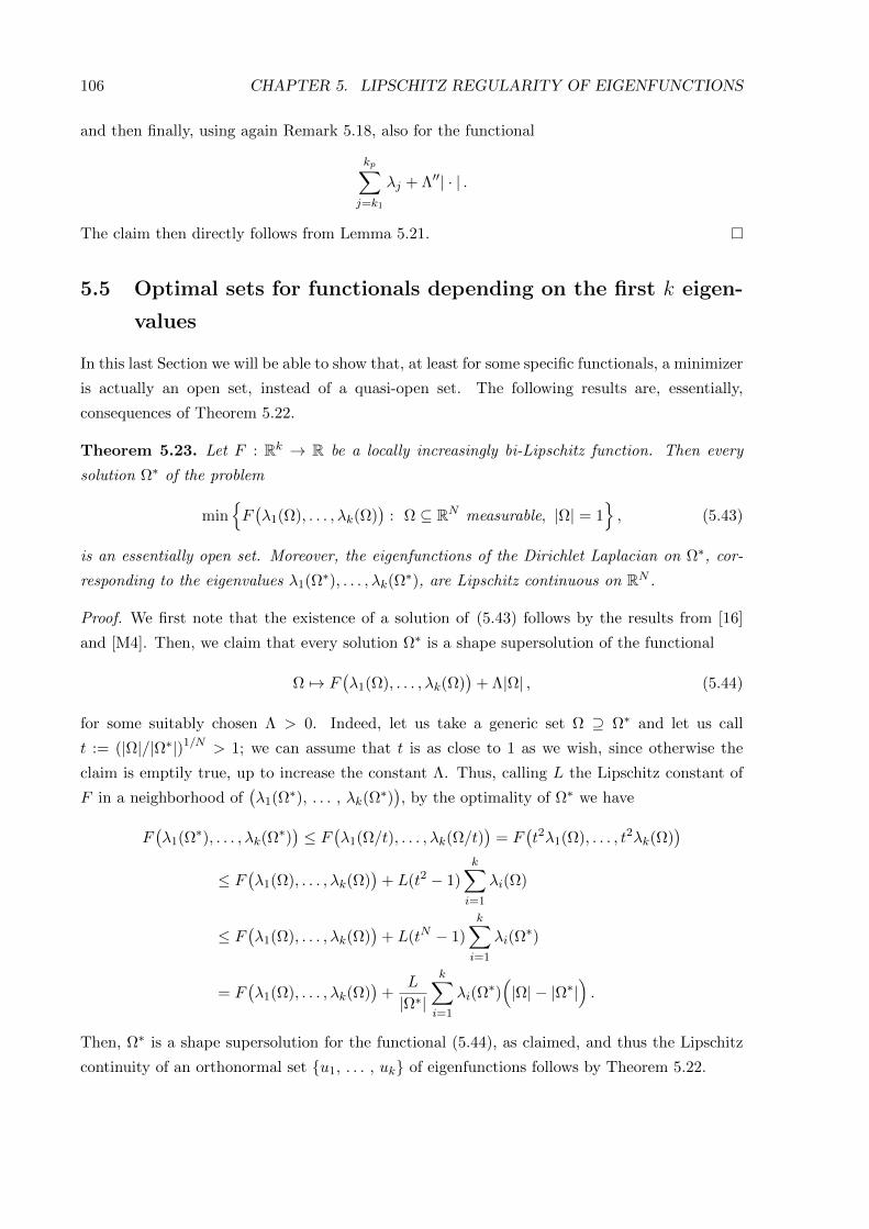
106 CHAPTER 5. LIPSCHITZ REGULARITY OF EIGENFUNCTIONS
and then finally, using again Remark 5.18, also for the functional
kp∑j=k1
λj + Λ′′| · | .
The claim then directly follows from Lemma 5.21.
5.5 Optimal sets for functionals depending on the first k eigen-
values
In this last Section we will be able to show that, at least for some specific functionals, a minimizer
is actually an open set, instead of a quasi-open set. The following results are, essentially,
consequences of Theorem 5.22.
Theorem 5.23. Let F : Rk → R be a locally increasingly bi-Lipschitz function. Then every
solution Ω∗ of the problem
minF(λ1(Ω), . . . , λk(Ω)
): Ω ⊆ RN measurable, |Ω| = 1
, (5.43)
is an essentially open set. Moreover, the eigenfunctions of the Dirichlet Laplacian on Ω∗, cor-
responding to the eigenvalues λ1(Ω∗), . . . , λk(Ω∗), are Lipschitz continuous on RN .
Proof. We first note that the existence of a solution of (5.43) follows by the results from [16]
and [M4]. Then, we claim that every solution Ω∗ is a shape supersolution of the functional
Ω 7→ F(λ1(Ω), . . . , λk(Ω)
)+ Λ|Ω| , (5.44)
for some suitably chosen Λ > 0. Indeed, let us take a generic set Ω ⊇ Ω∗ and let us call
t := (|Ω|/|Ω∗|)1/N > 1; we can assume that t is as close to 1 as we wish, since otherwise the
claim is emptily true, up to increase the constant Λ. Thus, calling L the Lipschitz constant of
F in a neighborhood of(λ1(Ω∗), . . . , λk(Ω
∗)), by the optimality of Ω∗ we have
F(λ1(Ω∗), . . . , λk(Ω
∗))≤ F
(λ1(Ω/t), . . . , λk(Ω/t)
)= F
(t2λ1(Ω), . . . , t2λk(Ω)
)≤ F
(λ1(Ω), . . . , λk(Ω)
)+ L(t2 − 1)
k∑i=1
λi(Ω)
≤ F(λ1(Ω), . . . , λk(Ω)
)+ L(tN − 1)
k∑i=1
λi(Ω∗)
= F(λ1(Ω), . . . , λk(Ω)
)+
L
|Ω∗|
k∑i=1
λi(Ω∗)(|Ω| − |Ω∗|
).
Then, Ω∗ is a shape supersolution for the functional (5.44), as claimed, and thus the Lipschitz
continuity of an orthonormal set u1, . . . , uk of eigenfunctions follows by Theorem 5.22.
5.5. OPTIMAL SETS FOR SPECIAL FUNCTIONALS 107
The openness of the set Ω∗ follows by the observation that the open set
Ω∗∗ :=
k⋃i=1
uk 6= 0
is essentially contained in Ω∗ and has the same first k eigenvalues as Ω∗: indeed, these eigenvalues
are smaller than those of Ω∗ by the characterization (2.6) of the eigenvalues and thanks to the
functions ui, but also greater than those of Ω∗ because Ω∗∗ is essentially contained in Ω∗. By
the optimality of Ω∗ we deduce that |Ω∗∆Ω∗∗| = 0, i.e., Ω∗∗ is equivalent to Ω∗ and the proof is
completed.
Observe that, by the definition of the open set Ω∗∗ in the above proof, it follows that the
first k eigenvalues defined on the space H10 (Ω∗∗), and those defined on the classical Sobolev
space H10 (Ω∗∗), coincide. Thus, we have a solution of the shape optimization problem (5.43) in
its classical formulation.
Corollary 5.24. Let F : Rk → R be a locally increasingly bi-Lipschitz function. Then there is
a solution Ω∗ of the problem
minF(λ1(Ω), . . . , λk(Ω)
): Ω ⊆ RN open, |Ω| = 1
.
Moreover, the eigenfunctions of the Dirichlet Laplacian on Ω∗, corresponding to the eigenvalues
λ1(Ω∗), . . . , λk(Ω∗), are Lipschitz continuous on RN .
The openness can be obtained not only for sets minimizing (5.43), but also for shape super-
solutions.
Proposition 5.25. Let F : Rk → R be a locally increasingly bi-Lipschitz function, and let Ω∗
be a shape supersolution for the functional
Ω 7→ F(λ1(Ω), . . . , λk(Ω)
)+ Λ|Ω| . (5.45)
Then there is an open set Ω∗∗ ⊆ Ω∗ such that λi(Ω∗∗) = λi(Ω
∗) for i = 1, . . . , k, and which
is still a supersolution for the functional (5.45). Moreover, there exists a sequence of Lipschitz
orthonormal eigenfunctions corresponding to the first k eigenvalues in Ω∗∗.
Proof. Applying Theorem 5.22 to Ω∗, we find an orthonormal set of Lipschitz eigenfunctions
u1, u2, . . . , uk for Ω∗; then, as in Theorem 5.23, we define
Ω∗∗ :=k⋃i=1
ui 6= 0 ,
which is open since the functions ui are Lipschitz continuous. As before, Ω∗∗ is essentially
contained in Ω∗, thus it has bigger eigenvalues, and on the other hand the definition of eigenvalues
–together with the fact that each ui is by definition in H10 (Ω∗∗)– gives the opposite inequality.
108 CHAPTER 5. LIPSCHITZ REGULARITY OF EIGENFUNCTIONS
As a consequence, we conclude that λi(Ω∗) = λi(Ω
∗∗) for every i = 1, . . . , k. It is now immediate
to show that Ω∗∗ is also a shape supersolution for (5.45): indeed, for every Ω ⊇ Ω∗∗, we just
compute
F(λ1(Ω∗∗), . . . , λk(Ω
∗∗))
+ Λ|Ω∗∗| = F(λ1(Ω∗), . . . , λk(Ω
∗))
+ Λ|Ω∗| − Λ|Ω∗ \ Ω∗∗|
≤ F(λ1(Ω ∪ Ω∗), . . . , λk(Ω ∪ Ω∗)
)+ Λ|Ω ∪ Ω∗| − Λ|Ω∗ \ Ω∗∗|
≤ F(λ1(Ω), . . . , λk(Ω)
)+ Λ|Ω| .
Being then Ω∗∗ a shape supersolution for (5.45), and being the functions ui also eigenfunctions
for Ω∗∗, the proof is concluded.
For functionals of the form
Ω 7→ F(λk1(Ω), . . . , λkp(Ω)
),
depending on some non-consecutive eigenvalues λk1 , . . . , λkp , it is still possible to obtain that an
optimal sets Ω∗ for the problem
minF(λk1(Ω), . . . , λkp(Ω)
): Ω ⊆ RN measurable, |Ω| = 1
, (5.46)
is open, provided that an additional condition on the eigenvalues of Ω∗ is satisfied.
Proposition 5.26. Let F : Rp → R be a locally increasingly bi-Lipschitz function, 0 < k1 <
k2 < · · · < kp be natural numbers, and Ω∗ be a minimizer for the problem (5.46). If for
all j = 1, . . . , p one has λkj (Ω∗) > λkj−1(Ω∗), then Ω∗ is essentially open. Moreover all the
eigenfunctions corresponding to λkj (Ω∗), for j = 1, . . . , p are Lipschitz continuous on RN .
Proof. First of all, we remind that a minimizer for the problem (5.46) exists and is bounded,
and moreover it is also a shape supersolution of the functional F(λk1(Ω), . . . , λkp(Ω)
))+ Λ|Ω|
for a suitable Λ, exactly as in the proof of Theorem 5.23; thus, the second part of the claim
simply follows by Theorem 5.22, and it only remains to show that Ω∗ is essentially open.
Let us fix an orthonormal set of eigenfunctions ui, 1 ≤ i ≤ kp for the first kp eigenvalues
in Ω∗, and consider the family of indices
I :=i ≤ kp : λi(Ω
∗) = λkj (Ω∗), for some j
.
Recalling again Theorem 5.22, we know that for every i ∈ I the eigenfunction ui is Lipschitz
continuous, thus the set
ΩA :=
x ∈ RN :
∑i∈I
ui(x)2 > 0
is open, and of course essentially contained in Ω∗. Our aim is then to prove that N = Ω∗ \ ΩA
is negligible. Suppose, by contradiction, that |N | > 0 and let x ∈ N be a point of density one
for N , i.e.
limρ→0
|N ∩Bρ(x)||Bρ(x)|
= 1 .
5.5. OPTIMAL SETS FOR SPECIAL FUNCTIONALS 109
Since, for ρ → 0, the sets Ω∗ \ (N ∩ Bρ(x)) γ-converge to Ω∗ we have the convergence of the
spectra λk(Ω∗ \ (N ∩Bρ(x)))→ λk(Ω
∗), for every k ∈ N. Then, being λkj (Ω∗) > λkj−1(Ω∗), we
can choose ρ small enough such that the set Ω = Ω∗ \ (N ∩Bρ(x)) satisfies
λkj−1(Ω) < λkj (Ω∗), ∀ j = 1, . . . , p . (5.47)
We note now that for i ∈ I the eigenfunction ui belongs to H10 (Ω), and since Ω ⊆ Ω∗ we get
that ui satisfies the equation
−∆ui = λkj (Ω∗)ui, ui ∈ H1
0 (Ω) .
Thus, for each i ∈ I the number λi(Ω∗) is also in the spectrum of the Dirichlet Laplacian on Ω.
Combined with (5.47) and with the fact that Ω ⊆ Ω∗, this gives
λk(Ω) = λk(Ω∗), ∀ k = 1, . . . , kp .
Since for every ρ > 0 we have |N ∩ Bρ(x)| > 0, it follows that |Ω| < |Ω∗| = 1; by the strict
monotonicity of F , if we rescale Ω till volume 1 we get a competitor strictly better than Ω∗
in (5.46), which is a contradiction with the optimality of Ω∗.
Remark 5.27. Unfortunately, Proposition 5.26 provides the openness of optimal sets only up to
zero Lebesgue measure. Hence we have that H10 (Ω∗) = H1
0 (ΩA), but we do not know in general
if H10 (Ω∗) = H1
0 (ΩA); thus, it is not clear whether an open “classical” solution exists, where by
“classical” we refer to the case when the eigenvalues are considered in the standard H10 spaces,
and not in the modified H10 spaces. Keep in mind that this problem did not occur with the
situation of Theorem 5.23, as noticed right after its proof.

110 CHAPTER 5. LIPSCHITZ REGULARITY OF EIGENFUNCTIONS
Chapter 6
Connectedness of minimizers for
convex combinations of low
eigenvalues
6.1 Introduction
In this last Chapter of the Thesis, we deal with the problem of connectedness of minimizers
for a convex combination of the first three eigenvalues of Dirichlet Laplacian. In particular, for
α, β ∈ [0, 1] and α+ β ≤ 1, we consider
infαλ1(Ω) + βλ2(Ω) + (1− α− β)λ3(Ω) : Ω ⊂ RN , open, |Ω| ≤ 1, (6.1)
and we aim to understand for which values of α, β all the minimizers for (6.1) are connected.
When α = 1 and β = 0, problem (6.1) reduces to the minimization of the first eigenvalue, and
by the Faber-Krahn inequality (2.9), it is well known that the ball is the unique minimizer.
Hence, in this case, the minimizer -the ball- is connected in every dimension. On the other
hand, if we consider the case of α = 0 and β = 1, which means that we are minimizing the
second eigenvalue, the Krahn-Szego inequality (2.10) asserts that two equal disjoint balls are
the unique minimizer. In this case the disconnectedness of the optimal set is somehow intrinsic
in the problem: it is easy to see that if we impose a connectedness constraint and consider,
infλ2(Ω) : Ω ⊂ RN , open, connected, |Ω| ≤ 1
,
then there are no minimizers and the infimum equals the value of λ2 for two equal disjoint balls
of half measure each. It is in fact sufficient to consider as a minimizing sequence the two equal
balls connected with a very thin strip (of volume decreasing to zero).
Very little is known about the other cases: Wolf and Keller in [53] proved that in dimension
N = 2, 3 any minimizer for λ3(Ω) (which corresponds to α = β = 0 in (6.1)) is connected, by
111
112 CHAPTER 6. CONNECTEDNESS OF MINIMIZERS
showing that the ball has lower third eigenvalue than any disconnected set of the same measure.
For N ≥ 4 it is not known whether minimizers for λ3 are connected; Wolf and Keller conjectured
that three disjoint equal balls should be optimal.
The Chapter is organized as follow: after Section 6.2 in which we recall how eigenvalues of
balls can be computed, in Section 6.3 we state the main results and propose a conjecture for the
cases that we are not able to treat. In Section 6.4 we give the proof of the results for generic
dimension, while Section 6.5 is devoted to the two dimensional case, in which more informations
can be obtained.
6.2 Explicit computations of eigenvalues for balls
We recall here some explicit computations of the eigenvalues for balls in the two dimensional
setting. Let BR ⊂ R2 be the ball of radius R centered in the origin. We look for eigenvalues
(and eigenfunctions) in polar coordinates (ρ, ϑ), that means we search a real number λ and a
function u such that,
−∆u(ρ, ϑ) = λu(ρ, ϑ) and u(ρ = R,ϑ) = 0.
The first equation can be rewritten using the expression of Laplace operator in polar coordinates:
−uρρ(ρ, ϑ)− 1
ρuρ(ρ, ϑ)− 1
ρ2uϑϑ(ρ, ϑ) = λu(ρ, ϑ).
Using the usual technique of separation of variables, we look for a solution of the form u(ρ, ϑ) =
v(ρ)w(ϑ), that leads to the equation:
−w(ϑ)v′′(ρ)− 1
ρw(ϑ)v′(ρ)− 1
ρ2w′′(ϑ)v(ρ) = λv(ρ)w(ϑ).
Forgetting the zero solution, we can divide both the right and the left hand side by v(ρ)w(ϑ):
−ρ2 v′′(ρ)
v(ρ)− ρv
′(ρ)
v(ρ)− ρ2λ =
w′′(ϑ)
w(ϑ).
Since the two sides of the equality depends on different variables, the only chance to achieve a
solution is that they are both equals to a constant k:
w′′(ϑ) + kw(θ) = 0 with w(ϑ) = w(ϑ+ 2mπ) ∀m ∈ Z (6.2)
v′′(ρ) +1
ρv′(ρ) + (λ− k
ρ2)v(ρ) = 0 with v(R) = 0 and v′(0) = 0 (6.3)
The periodicity condition in equation (6.2) implies k = m2 and w(ϑ) = am cos(mϑ)+bm sin(mϑ)
for m ∈ N. Hence equation (6.3) for k = m2 becomes a Bessel differential equation.
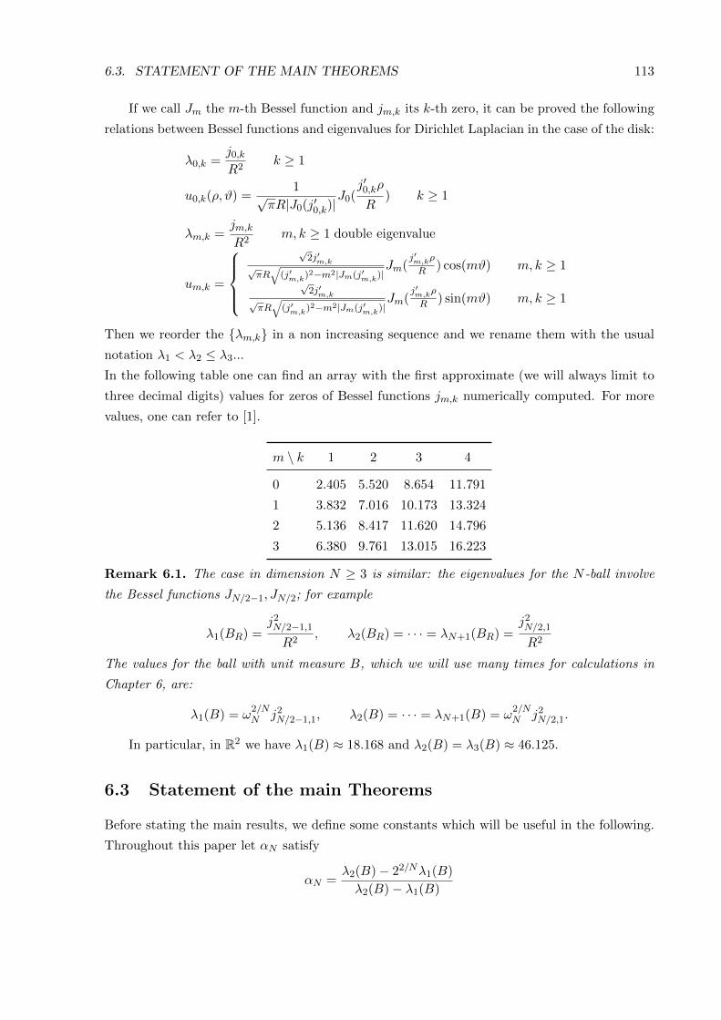
6.3. STATEMENT OF THE MAIN THEOREMS 113
If we call Jm the m-th Bessel function and jm,k its k-th zero, it can be proved the following
relations between Bessel functions and eigenvalues for Dirichlet Laplacian in the case of the disk:
λ0,k =j0,kR2
k ≥ 1
u0,k(ρ, ϑ) =1√
πR|J0(j′0,k)|J0(
j′0,kρ
R) k ≥ 1
λm,k =jm,kR2
m, k ≥ 1 double eigenvalue
um,k =
√
2j′m,k√πR
√(j′m,k)2−m2|Jm(j′m,k)|
Jm(j′m,kρ
R ) cos(mϑ) m, k ≥ 1√
2j′m,k√πR
√(j′m,k)2−m2|Jm(j′m,k)|
Jm(j′m,kρ
R ) sin(mϑ) m, k ≥ 1
Then we reorder the λm,k in a non increasing sequence and we rename them with the usual
notation λ1 < λ2 ≤ λ3...
In the following table one can find an array with the first approximate (we will always limit to
three decimal digits) values for zeros of Bessel functions jm,k numerically computed. For more
values, one can refer to [1].
m \ k 1 2 3 4
0 2.405 5.520 8.654 11.791
1 3.832 7.016 10.173 13.324
2 5.136 8.417 11.620 14.796
3 6.380 9.761 13.015 16.223
Remark 6.1. The case in dimension N ≥ 3 is similar: the eigenvalues for the N -ball involve
the Bessel functions JN/2−1, JN/2; for example
λ1(BR) =j2N/2−1,1
R2, λ2(BR) = · · · = λN+1(BR) =
j2N/2,1
R2
The values for the ball with unit measure B, which we will use many times for calculations in
Chapter 6, are:
λ1(B) = ω2/NN j2
N/2−1,1, λ2(B) = · · · = λN+1(B) = ω2/NN j2
N/2,1.
In particular, in R2 we have λ1(B) ≈ 18.168 and λ2(B) = λ3(B) ≈ 46.125.
6.3 Statement of the main Theorems
Before stating the main results, we define some constants which will be useful in the following.
Throughout this paper let αN satisfy
αN =λ2(B)− 22/Nλ1(B)
λ2(B)− λ1(B)
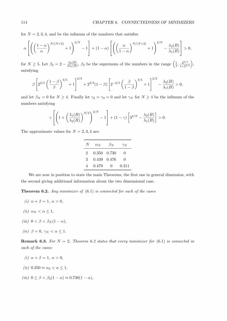
114 CHAPTER 6. CONNECTEDNESS OF MINIMIZERS
for N = 2, 3, 4, and be the infimum of the numbers that satisfies
α
((1− αα
)N/(N+2)
+ 1
)2/N
− 1
+ (1− α)
(( α
1− α
)N/(N+2)
+ 1
)2/N
− λ2(B)
λ1(B)
> 0,
for N ≥ 5. Let β2 = 2 − λ2(B)2λ1(B) , β3 be the supremum of the numbers in the range
(13 ,
22/3
1+22/3
),
satisfying
β
[22/5
(1− ββ
)3/5
+ 1
]2/3
+ 22/3(1− β)
[2−2/5
(β
1− β
)3/5
+ 1
]2/3
− λ2(B)
λ1(B)> 0,
and let βN = 0 for N ≥ 4. Finally let γ2 = γ3 = 0 and let γN for N ≥ 4 be the infimum of the
numbers satisfying
γ
(1 +
(λ1(B)
λ2(B)
)N/2)2/N
− 1
+ (1− γ)
[32/N − λ2(B)
λ1(B)
]> 0.
The approximate values for N = 2, 3, 4 are:
N αN βN γN
2 0.350 0.730 0
3 0.439 0.476 0
4 0.479 0 0.311
We are now in position to state the main Theorems, the first one in general dimension, with
the second giving additional information about the two dimensional case.
Theorem 6.2. Any minimizer of (6.1) is connected for each of the cases
(i) α+ β = 1, α > 0,
(ii) αN < α ≤ 1,
(iii) 0 < β < βN (1− α),
(iv) β = 0, γN < α ≤ 1.
Remark 6.3. For N = 2, Theorem 6.2 states that every minimizer for (6.1) is connected in
each of the cases:
(i) α+ β = 1, α > 0,
(ii) 0.350 ≈ α2 < α ≤ 1,
(iii) 0 ≤ β < β2(1− α) ≈ 0.730(1− α),
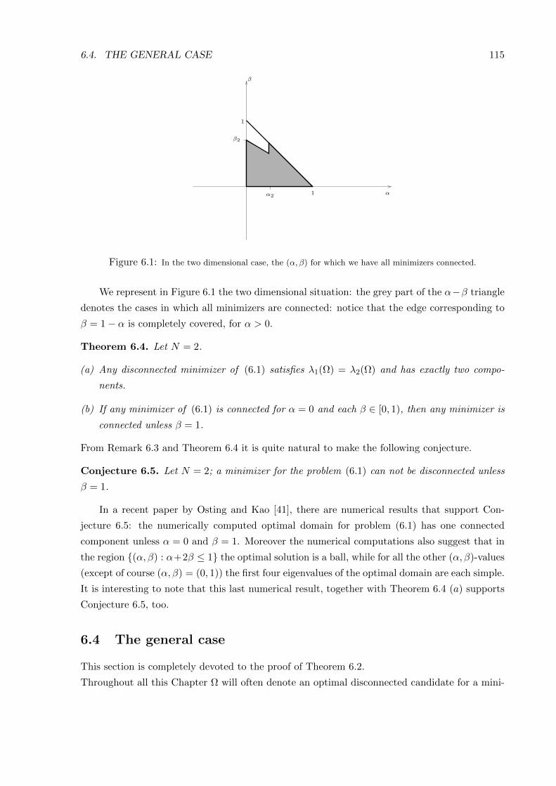
6.4. THE GENERAL CASE 115
1
α1
β
α2
β2
Figure 6.1: In the two dimensional case, the (α, β) for which we have all minimizers connected.
We represent in Figure 6.1 the two dimensional situation: the grey part of the α−β triangle
denotes the cases in which all minimizers are connected: notice that the edge corresponding to
β = 1− α is completely covered, for α > 0.
Theorem 6.4. Let N = 2.
(a) Any disconnected minimizer of (6.1) satisfies λ1(Ω) = λ2(Ω) and has exactly two compo-
nents.
(b) If any minimizer of (6.1) is connected for α = 0 and each β ∈ [0, 1), then any minimizer is
connected unless β = 1.
From Remark 6.3 and Theorem 6.4 it is quite natural to make the following conjecture.
Conjecture 6.5. Let N = 2; a minimizer for the problem (6.1) can not be disconnected unless
β = 1.
In a recent paper by Osting and Kao [41], there are numerical results that support Con-
jecture 6.5: the numerically computed optimal domain for problem (6.1) has one connected
component unless α = 0 and β = 1. Moreover the numerical computations also suggest that in
the region (α, β) : α+2β ≤ 1 the optimal solution is a ball, while for all the other (α, β)-values
(except of course (α, β) = (0, 1)) the first four eigenvalues of the optimal domain are each simple.
It is interesting to note that this last numerical result, together with Theorem 6.4 (a) supports
Conjecture 6.5, too.
6.4 The general case
This section is completely devoted to the proof of Theorem 6.2.
Throughout all this Chapter Ω will often denote an optimal disconnected candidate for a mini-
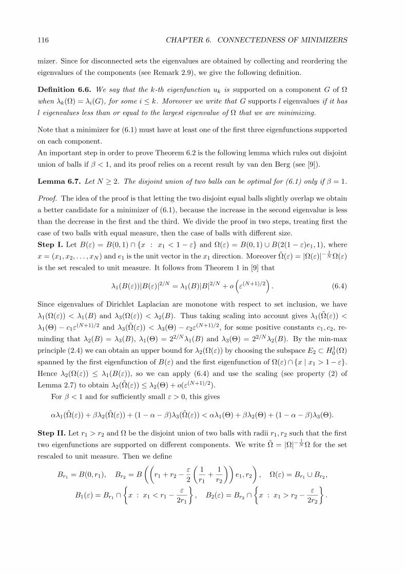
116 CHAPTER 6. CONNECTEDNESS OF MINIMIZERS
mizer. Since for disconnected sets the eigenvalues are obtained by collecting and reordering the
eigenvalues of the components (see Remark 2.9), we give the following definition.
Definition 6.6. We say that the k-th eigenfunction uk is supported on a component G of Ω
when λk(Ω) = λi(G), for some i ≤ k. Moreover we write that G supports l eigenvalues if it has
l eigenvalues less than or equal to the largest eigenvalue of Ω that we are minimizing.
Note that a minimizer for (6.1) must have at least one of the first three eigenfunctions supported
on each component.
An important step in order to prove Theorem 6.2 is the following lemma which rules out disjoint
union of balls if β < 1, and its proof relies on a recent result by van den Berg (see [9]).
Lemma 6.7. Let N ≥ 2. The disjoint union of two balls can be optimal for (6.1) only if β = 1.
Proof. The idea of the proof is that letting the two disjoint equal balls slightly overlap we obtain
a better candidate for a minimizer of (6.1), because the increase in the second eigenvalue is less
than the decrease in the first and the third. We divide the proof in two steps, treating first the
case of two balls with equal measure, then the case of balls with different size.
Step I. Let B(ε) = B(0, 1) ∩ x : x1 < 1 − ε and Ω(ε) = B(0, 1) ∪ B(2(1 − ε)e1, 1), where
x = (x1, x2, . . . , xN ) and e1 is the unit vector in the x1 direction. Moreover Ω(ε) = |Ω(ε)|−1N Ω(ε)
is the set rescaled to unit measure. It follows from Theorem 1 in [9] that
λ1(B(ε))|B(ε)|2/N = λ1(B)|B|2/N + o(ε(N+1)/2
). (6.4)
Since eigenvalues of Dirichlet Laplacian are monotone with respect to set inclusion, we have
λ1(Ω(ε)) < λ1(B) and λ3(Ω(ε)) < λ2(B). Thus taking scaling into account gives λ1(Ω(ε)) <
λ1(Θ) − c1ε(N+1)/2 and λ3(Ω(ε)) < λ3(Θ) − c2ε
(N+1)/2, for some positive constants c1, c2, re-
minding that λ2(B) = λ3(B), λ1(Θ) = 22/Nλ1(B) and λ3(Θ) = 22/Nλ2(B). By the min-max
principle (2.4) we can obtain an upper bound for λ2(Ω(ε)) by choosing the subspace E2 ⊂ H10 (Ω)
spanned by the first eigenfunction of B(ε) and the first eigenfunction of Ω(ε)∩ x | x1 > 1− ε.Hence λ2(Ω(ε)) ≤ λ1(B(ε)), so we can apply (6.4) and use the scaling (see property (2) of
Lemma 2.7) to obtain λ2(Ω(ε)) ≤ λ2(Θ) + o(ε(N+1)/2).
For β < 1 and for sufficiently small ε > 0, this gives
αλ1(Ω(ε)) + βλ2(Ω(ε)) + (1− α− β)λ3(Ω(ε)) < αλ1(Θ) + βλ2(Θ) + (1− α− β)λ3(Θ).
Step II. Let r1 > r2 and Ω be the disjoint union of two balls with radii r1, r2 such that the first
two eigenfunctions are supported on different components. We write Ω = |Ω|−1N Ω for the set
rescaled to unit measure. Then we define
Br1 = B(0, r1), Br2 = B
((r1 + r2 −
ε
2
(1
r1+
1
r2
))e1, r2
), Ω(ε) = Br1 ∪Br2 ,
B1(ε) = Br1 ∩x : x1 < r1 −
ε
2r1
, B2(ε) = Br2 ∩
x : x1 > r2 −
ε
2r2
.
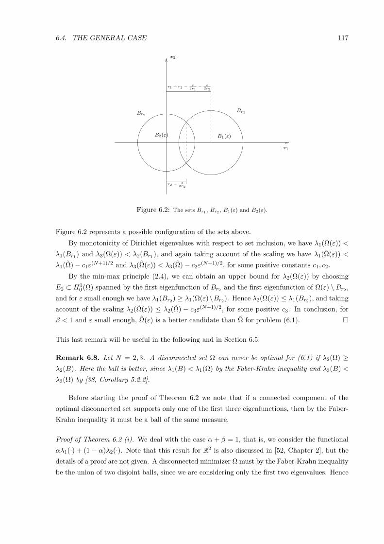
6.4. THE GENERAL CASE 117
x1
x2
r1 + r2 − ε2r1− ε
2r2
Br2
B2(ε)
Br1
B1(ε)
r2 − ε2r2
Figure 6.2: The sets Br1 , Br2 , B1(ε) and B2(ε).
Figure 6.2 represents a possible configuration of the sets above.
By monotonicity of Dirichlet eigenvalues with respect to set inclusion, we have λ1(Ω(ε)) <
λ1(Br1) and λ3(Ω(ε)) < λ2(Br1), and again taking account of the scaling we have λ1(Ω(ε)) <
λ1(Ω)− c1ε(N+1)/2 and λ3(Ω(ε)) < λ3(Ω)− c2ε
(N+1)/2, for some positive constants c1, c2.
By the min-max principle (2.4), we can obtain an upper bound for λ2(Ω(ε)) by choosing
E2 ⊂ H10 (Ω) spanned by the first eigenfunction of Br2 and the first eigenfunction of Ω(ε) \Br2 ,
and for ε small enough we have λ1(Br2) ≥ λ1(Ω(ε)\Br2). Hence λ2(Ω(ε)) ≤ λ1(Br2), and taking
account of the scaling λ2(Ω(ε)) ≤ λ2(Ω) − c3ε(N+1)/2, for some positive c3. In conclusion, for
β < 1 and ε small enough, Ω(ε) is a better candidate than Ω for problem (6.1).
This last remark will be useful in the following and in Section 6.5.
Remark 6.8. Let N = 2, 3. A disconnected set Ω can never be optimal for (6.1) if λ2(Ω) ≥λ2(B). Here the ball is better, since λ1(B) < λ1(Ω) by the Faber-Krahn inequality and λ3(B) <
λ3(Ω) by [38, Corollary 5.2.2].
Before starting the proof of Theorem 6.2 we note that if a connected component of the
optimal disconnected set supports only one of the first three eigenfunctions, then by the Faber-
Krahn inequality it must be a ball of the same measure.
Proof of Theorem 6.2 (i). We deal with the case α + β = 1, that is, we consider the functional
αλ1(·) + (1 − α)λ2(·). Note that this result for R2 is also discussed in [52, Chapter 2], but the
details of a proof are not given. A disconnected minimizer Ω must by the Faber-Krahn inequality
be the union of two disjoint balls, since we are considering only the first two eigenvalues. Hence
118 CHAPTER 6. CONNECTEDNESS OF MINIMIZERS
an immediate application of Lemma 6.7 rules out this configuration in any dimension when
α > 0, so we conclude.
Remark 6.9. It is actually possible to give a different proof of the connectedness of the mini-
mizers for the problem
infαλ1(Ω) + (1− α)λ2(Ω) : Ω ⊆ RN , open, with |Ω| ≤ 1
, (6.5)
for α > 0, that does not involve the use of Theorem 1 from [9]. It is easy to see that the optimal
disconnected set for problem (6.5) if α ∈ (1/2, 1] is made by two disjoint ball of different measure
and hence can never be optimal by Step II of Lemma 6.7. On the other hand when α ∈ (0, 1/2]
the best disconnected set is the disjoint union of two equal balls with half measure, Θ. We give
here a different proof of the fact that Θ can not be optimal for (6.5) unless α = 0. It is clearly
sufficient to focus on the case α ∈ (0, 1/2].
We introduce the set
E =
(λ1(Ω), λ2(Ω)) : Ω ⊆ RN open, with |Ω| = 1.
For a description of many properties of this set and a numerical approximation of it we refer
to [21] or to [38, Chapter 6.4]. The property which interests us deals with the lower part of the
boundary of E, the curve C that joins the point A = (λ1(Θ), λ2(Θ)) and B = (λ1(B), λ2(B)) (see
Figure 6.3).
B
A
E
αx+ (1− α)y = a
C
λ2
λ1
Figure 6.3: The set E .
Wolf and Keller in [53] proved that the curve C must be vertical at the point B by a pertur-
bation argument with nearly circular domains. They also suggested that C should be horizontal
at A, and this was proved recently by Brasco, Nitsch and Pratelli in [12]. This is the crucial
point of our proof, as a minimizer for the convex combination αλ1(Ω) + (1 − α)λ2(Ω) is given
6.4. THE GENERAL CASE 119
by the set corresponding to the first point in which the straight line αx + (1 − α)y = a touches
E, by increasing a. In particular, for α = 0 this line is y = λ2(Θ) = 2λ1(B) by the Krahn-Szego
inequality. On the other hand, for all α ∈ (0, 1/2), it is possible to find a set Ω that is linked
to a line of the form αx + (1 − α)y = aα, with aα < λ2(Θ) = 2λ1(B), since the curve C has
horizontal tangent. Hence Θ can not be the minimizer for (6.5) unless α = 0.
Proof of Theorem 6.2 (ii). We need a different argument from the one used in the proof of part
(i), but start again from the case α + β = 1. The case α = 1 was already solved by the
Faber-Krahn inequality (2.9). Again a disconnected minimizer Ω must be the union of two
disjoint balls. Without loss of generality, we suppose that the ball supporting u1 has measure
m ≤ 1, while the other one (supporting u2) has measure 1 −m. Having in mind the scaling of
eigenvalues, it is clear that m ≥ 1/2 and we have
αλ1(Ω) + (1− α)λ2(Ω) = λ1(B)
(α
m2/N+
1− α(1−m)2/N
).
First of all we consider the case when α ∈ (12 , 1). By minimizing in m in the previous expression
to obtain a lower bound and comparing with the value for the unit ball rules out this configuration
if
αλ1(B)
[(1− αα
)N/(N+2)
+ 1
]2/N
+ (1− α)λ1(B)
[(α
1− α
)N/(N+2)
+ 1
]2/N
(6.6)
> αλ1(B) + (1− α)λ2(B),
that is, when the function fN : (0, 1)→ R,
fN (α) = α
[(
1− αα
) NN+2
+ 1
] 2N
− 1
+ (1− α)
[(
α
1− α
) NN+2
+ 1
] 2N
− λ2(B)
λ1(B)
is positive. The following property of fN (α) is important for our analysis.
Claim 6.A.
For every N ∈ N, there exists αN ∈ (0, 1) such that
fN (α) < 0 if α ∈ (0, αN ) and fN (α) > 0 if α ∈ (αN , 1).
Proof of Claim 6.A. We introduce the increasing function ψ : [0, 1)→ [0,∞):
ψ(α) =α
1− α,
and φN : (0,∞)→ R
φN (t) = t
[(
1
t
) NN+2
+ 1
] 2N
− 1
+
[tNN+2 + 1
] 2N − λ2(B)
λ1(B)
,
120 CHAPTER 6. CONNECTEDNESS OF MINIMIZERS
so that fN (α) = (1 − α)φN (ψ(α)), for α ∈ (0, 1). Hence the sign of fN in the interval (0, 1) is
the same as that of φN in the interval (0,∞). We note that φN is the sum of two functions,
where the second one,
t 7→(tNN+2 + 1
) 2N − λ2(B)
λ1(B),
is strictly increasing. The first one,
t 7→ t
[(
1
t
) NN+2
+ 1
] 2N
− 1
=: φ1N (t),
is also strictly increasing, since we have:
d
dtφ1N (t) =
[(
1
t
) NN+2
+ 1
] 2N
− 1
− 2
N + 2t−
NN+2
[(1
t
) NN+2
+ 1
] 2N−1
,
that is positive when
1 +N
N + 2t−
NN+2 >
[(1
t
) NN+2
+ 1
]1− 2N
.
The above inequality holds, since t 7→ t1−2/N is concave and thus[(1
t
) NN+2
+ 1
]1− 2N
< 1 +N − 2
N
(1
t
) NN+2
< 1 +N
N + 2
(1
t
) NN+2
,
where we used also the inequality (N − 2)/N < N/(N + 2). So φN is the sum of two strictly
increasing functions and thus it has the same property. Hence φN can change sign only once in
(0,∞). We note that
limt→0+
φN (t) = 1− λ2(B)
λ1(B)< 0 and lim
t→∞φN (t) = +∞,
so there exists an unique tN ∈ (0,∞) such that
φN (t) < 0 if t ∈ (0, tN ) and φN (t) > 0 if t ∈ (tN ,∞).
In conclusion the thesis follows setting αN = ψ−1(tN ).
Keep in mind that, for all N ≥ 2, fN (α) > 0 if and only if (6.6) holds for α. We can
compute
f2
(1
2
)=
1
2
((1 + 1)− 1
)+
1
2
[(1 + 1)− λ2(B)
λ1(B)
]≈ 0.230 > 0,
f3
(1
2
)=
1
2
((1 + 1)2/3 − 1
)+
1
2
[(1 + 1)2/3 − λ2(B)
λ1(B)
]≈ 0.065 > 0,
f4
(1
2
)=
1
2
((1 + 1)1/2 − 1
)+
1
2
[(1 + 1)1/2 − λ2(B)
λ1(B)
]≈ 0.016 > 0,
6.4. THE GENERAL CASE 121
where we used that
λ2(B)
λ1(B)≈
2.539 if N = 2,
2.044 if N = 3,
1.796 if N = 4.
Then, by Claim 6.A, for N ≤ 4 we have that αN < 1/2, since fN (1/2) > 0. Hence fN (α) > 0
for all α ∈ (1/2, 1) and thus (6.6) holds in that range.
When N ≥ 5, we define αN = inf α ∈ (1/2, 1) : (6.6) holds and Claim 6.A assures that (6.6)
is true for all α ∈ (αN , 1).
Now we deal with the case when α ∈ (0, 12 ]. The constraint m ≥ 1/2 implies that the optimal
disconnected configuration consists in two disjoint balls of equal measure, since in this case we
have
λ1(B)22/n = αλ1(Θ) + (1− α)λ2(Θ) < λ1(B)
(α
m2/n+
1− α(1−m)2/n
).
This is ruled out by comparison with the unit ball when
λ1(B)22/N > αλ1(B) + (1− α)λ2(B), (6.7)
and we call, for N ≤ 4, αN = λ2(B)−22N λ1(B)
λ2(B)−λ1(B) , so that if α ∈ (αN , 1/2], then (6.7) holds. On the
other hand, if N ≥ 5, (6.7) is never true.
In conclusion, putting together the discussion for α ∈ (0, 1/2] and for α ∈ (1/2, 1), we have that
(a) For N ≤ 4 the ball is a better candidate for problem (6.1) than any disconnected minimizer
if α ∈ (αN , 1/2] ∪ (1/2, 1).
(b) For N ≥ 5 the ball is a better candidate for problem (6.1) than any disconnected minimizer
if α ∈ (αN , 1).
Thus we define αN = αN if N ≥ 5 and αN = αN if N ≤ 4; hence we have that the ball is better
than any disconnected set for 1 ≥ α > αN .
Finally to extend beyond the situation α+ β = 1, just note that for 1 ≥ α > αN
αλ1(Ω) + βλ2(Ω) + (1− α− β)λ3(Ω) ≥ αλ1(Ω) + (1− α)λ2(Ω)
> αλ1(B) + (1− α)λ2(B) = αλ1(B) + βλ2(B) + (1− α− β)λ3(B),
using the fact that λ2(Ω) ≤ λ3(Ω) while λ2(B) = λ3(B), so we conclude.
Proof of Theorem 6.2 (iii). The case α = 0. We first consider the case α = 0, that is, we
deal with the functional βλ2(·) + (1 − β)λ3(·). First of all we find out the best disconnected
configuration.
Claim 6.B.
Let α = 0. A disconnected minimizer is made by a ball supporting u2 and another set supporting
u1 and u3.
122 CHAPTER 6. CONNECTEDNESS OF MINIMIZERS
Proof of Claim 6.B. At first, we consider the configuration made by a set supporting u1, u2 and
a ball supporting u3. Since λ1 does not appear in the functional, it is better to have three balls
by applying Krahn-Szego inequality (2.10) to the set supporting u1 and u2. Note that the new
set, made by three disjoint balls, is as in the statement of the claim.
On the other hand an optimal configuration made by a ball supporting u1 and by another set
supporting u2, u3 should satisfy λ1(Ω) = λ2(Ω), since λ1 is not involved in the minimization.
Up to switch λ1 and λ2, we are in a configuration made by a ball supporting u2 and another set
supporting u1, u3 so the claim is proved.
Thanks to Claim 6.B, it remains only to rule out a disconnected minimizer made by a ball
supporting u2, which we suppose to have measure m (hence λ2(Ω) = λ1(B)
m2/n ) and a set supporting
u1 and u3 (which must have measure 1−m). Unfortunately, we are able to find out informations
only when n = 2, 3. First of all we note that m ≤ 1/2, otherwise, by the Faber-Krahn inequality,
λ1(Ω) > λ2(Ω). Moreover, using Remark 6.8, it must happen that λ2(B) > λ2(Ω), which implies
λ1(B)
m2/N< λ2(B), that is, m >
(λ1(B)
λ2(B)
)N/2,
that assures m ≥ 1/3 for N = 2, 3. For β ∈ [0, 1), the Krahn-Szego inequality gives the lower
bound
βλ2(Ω) + (1− β)λ3(Ω) ≥ λ1(B)
(β
m2/N+
22/N (1− β)
(1−m)2/N
). (6.8)
We are interested in minimizing the left hand side of (6.8) with respect to m, in order to improve
the lower bound. We define
m(β) =
[22/(N+2)
(1− ββ
)N/(N+2)
+ 1
]−1
,
and note that the right hand side of (6.8) is decreasing in (0,m(β)) and increasing in (m(β),∞).
Moreover, we have that
m(β) ≤ 1
3if β ∈
[0,
1
3
]and m(β) ≥ 1
2if β ∈
[2
2N
1 + 22N
, 1
),
so that (from the constraints on m) in this two ranges the right hand side of (6.8) is minimal for
m = 1/3 and m = 1/2 respectively. On the other hand, when β ∈(
13 ,
22N
1+22N
), the right hand
side of (6.8) is minimal for m = m(β).
We are now in position to compare the lower bound for βλ2(Ω) + (1− β)λ3(Ω) with βλ2(B) +
(1− β)λ3(B) = λ2(B).
For β ∈ [0, 1/3] we have
λ2(B) < 32N λ1(B) ≤ βλ2(Ω) + (1− β)λ3(Ω),
6.4. THE GENERAL CASE 123
hence in this range, for N = 2, 3, the ball is a better candidate than any disconnected set for
problem (6.1).
Now we deal with the case when β ∈(
13 ,
22/N
1+22/N
). Substituting the optimal values for m in (6.8)
and comparing with βλ2(B) + (1 − β)λ3(B) = λ2(B) gives connectedness for the whole range
when N = 2, since
λ2(B) < λ1(B)
[β
(√2(1− β)
β+ 1
)+ 2(1− β)
(√β
2(1− β)+ 1
)]∀β ∈
(1
3,2
3
).
On the other hand, for n = 3, we have connectedness when
λ2(B) < λ1(B)
β[
22/5
(1− ββ
)3/5
+ 1
]2/3
+ 22/3(1− β)
[2−2/5
(β
1− β
)3/5
+ 1
]2/3 .
(6.9)
In order to study this situation, we start by considering the function g : (0, 1)→ R
g(β) = β
[22/5
(1− ββ
)3/5
+ 1
]2/3
+ 22/3(1− β)
[2−2/5
(β
1− β
)3/5
+ 1
]2/3
− λ2(B)
λ1(B),
and note that (6.9) holds for a β ∈(
13 ,
22/3
1+22/3
)if and only if g(β) > 0. The function g is concave
in its whole domain (0, 1), since it is possible to compute
g′′(β) = −
(29/5
25β−11/5(1− β)−2/5
)[22/5
(1− ββ
)3/5
+ 1
]−4/3
− 29/5
25
(β−3/5(1− β)−7/5 + β−8/5(1− β)−2/5
)[22/5
(1− ββ
)3/5
+ 1
]−1/3
− 213/15
25β−4/5(1− β)−11/5
[2−2/5
(β
1− β
)3/5
+ 1
]−4/3
− 234/15
25
(β−2/5(1− β)−8/5 + β−7/5(1− β)−3/5
)[2−2/5
(β
1− β
)3/5
+ 1
]−1/3
< 0.
Moreover we have that
g(1/3) ≈ 0.036 > 0, while g
(22/3
1 + 22/3
)≈ −0.094 < 0,
hence we define β3 = supβ ∈
(13 ,
22/3
1+22/3
): g(β) > 0
and notice that the set
β ∈
(1
3,
22/3
1 + 22/3
): (6.9) holds
= (1/3, β3)
is a nonempty interval.
124 CHAPTER 6. CONNECTEDNESS OF MINIMIZERS
At last, we consider also the case when β ∈[
22/N
1+22/N , 1)
. As we pointed out above, here we
obtain the minimum in the right hand side of (6.8) for m = 1/2. Comparing again with the
functional for the ball, in the two dimensional case, we have connectedness when 2/3 ≤ β < β2,
since we have
λ2(B) < 2(2− β)λ1(B).
On the other hand, unfortunately, we do not obtain additional informations when N = 3.
Putting all the above information together, we conclude connectedness for:
N = 2 : β ∈ [0, β2) ≈ [0, 0.730),
N = 3 : β ∈ [0, β3) ≈ [0, 0.476).
The case 0 < β < βN (1− α). Recall from the above (case α = 0) that
ηλ2(Ω) + (1− η)λ3(Ω) > ηλ2(B) + (1− η)λ3(B),
for η ∈ [0, βN ). This implies, with the choice η = β1−α ,
β
1− αλ2(Ω) +
(1− α− β)
1− αλ3(Ω) >
β
1− αλ2(B) +
(1− α− β)
1− αλ3(B),
for β1−α ∈ [0, βN ), and so
βλ2(Ω) + (1− α− β)λ3(Ω) > βλ2(B) + (1− α− β)λ3(B),
for β ∈ [0, βN (1 − α)). Together with λ1(Ω) ≥ λ1(B) this concludes the proof of Theorem 6.2
(iii).
Proof of Theorem 6.2 (iv): the case β = 0. We finally consider the case β = 0, that is, we deal
with the functional αλ1(·) + (1 − α)λ3(·). To prove connectedness we first look for the best
disconnected set.
Claim 6.C.
Let β = 0. A disconnected minimizer is made by a ball supporting u3 and another set supporting
u1, u2.
Proof of Claim 6.C. First of all we note that a configuration with a ball supporting the first
eigenfunction and a set supporting the others would be three balls using the Krahn-Szego in-
equality (2.10) on this last set. A set made by three balls is as required in the claim.
On the other hand an optimal configuration with a ball supporting the second eigenvalue would
have λ2(Ω) = λ3(Ω), as scaling down the ball to obtain this does not effect λ1(Ω), λ3(Ω). Up to
switch λ2 and λ3 we are in a configuration with a ball supporting u3 and another set supporting
u1, u2. So the claim is proved.
6.4. THE GENERAL CASE 125
We can now focus on a disconnected set made by a ball with measure m supporting u3 and
a set (with measure 1−m) supporting u1, u2; we aim to rule it out. This is done by obtaining
lower bounds for the first and third eigenvalues and using comparison with a ball. By the
scaling (see property (2) of Lemma 2.7), we have λ3(Ω) = λ1(B)
m2/N , while the Faber-Krahn and the
Krahn-Szego inequalities respectively give
λ1(Ω) ≥ λ1(B)
(1−m)2/Nand
λ1(B)
m2/N= λ3(Ω) ≥ λ2(Ω) ≥ 22/N λ1(B)
(1−m)2/N, (6.10)
which implies 1m ≥ 3, and so m ≤ 1
3 . By [38, Corollary 5.2.2] we have that, since Ω is discon-
nected, for N = 2, 3
λ3(B) = λ2(B) ≤ λ3(Ω).
By the Faber-Krahn inequality, the ball strictly lowers the first eigenvalue, so we rule out this
configuration for all α ∈ [0, 1] when N = 2, 3.
For N ≥ 4 we must be more precise and obtain only partial estimates. If λ3(Ω) = λ1(B)
m2/N ≥λ2(B)
(1−m)2/N , then as we assume β = 0, the set supporting the first two eigenvalues should be a ball
B1. This would contradict the optimality of Ω, as we would have λ3(B1) = λ2(B1) ≤ λ3(Ω) and
|B1| < 1. So we conclude λ1(B)
m2/N < λ2(B)
(1−m)2/N , hence m >mN/20
1+mN/20
, which gives the bound
1
1−m> 1 +m
N/20 . (6.11)
Taking into account (6.10), (6.11) and the estimate m ≥ 1/3, we obtain
αλ1(Ω) + (1− α)λ3(Ω) ≥ αλ1(B)(
1 +mN/20
)2/N+ (1− α)λ1(B)32/N . (6.12)
By comparing the lower bound (6.12) with αλ1(B) + (1− α)λ3(B) we deduce that a minimizer
is connected when γN < α ≤ 1 and the proof of Theorem 6.2 (iv) is concluded. We have
connectedness, for example, in the following ranges:
N = 2 : α ∈ [0, 1],
N = 3 : α ∈ [0, 1],
N = 4 : α ∈ (γ4, 1] ≈ (0.311, 1],
N = 5 : α ∈ (γ5, 1] ≈ (0.467, 1],
N = 6 : α ∈ (γ6, 1] ≈ (0.547, 1].
126 CHAPTER 6. CONNECTEDNESS OF MINIMIZERS
6.5 The two dimensional case
We start this section with a lemma which rules out a minimizer for problem (6.1) with three
connected components when n = 2. We remind that we call F(·) = αλ1(·) + βλ2(·) + (1− α−β)λ3(·), while G is the same functional for α = 0, in order to avoid confusion.
Lemma 6.10. Let N = 2. Any disconnected minimizer of (6.1) has at most two connected
components.
Proof. For the case α + β = 1, which corresponds to the functional αλ1(·) + (1 − α)λ2(·), it is
clear that a minimizer has at most two components since only the first two eigenvalues are into
play. For α + β < 1 the Faber-Krahn inequality implies that a disconnected minimizer with
three components would be the union of three disjoint balls. If α > 0, it is possible to apply
Lemma 6.7 to the union of the balls supporting the second and the third eigenfunctions, thus
ruling out this configuration. For α = 0 (that is, for the functional βλ2(·) + (1 − β)λ3(·)) this
argument does not work, since we can lower only λ1 which is not into play, while neither λ2 nor
λ3 are lowered. Hence we rule out the configuration with three connected components only for
n = 2, by comparing it with B and Θ.
Let G(·) = βλ2(·) + (1 − β)λ3(·), and write Ωi, i = 1, 2, 3, for the three components of Ω.
Assuming λi(Ω) = λ1(Ωi) for i = 1, 2, 3 gives |Ω1| ≥ |Ω2| ≥ |Ω3|. We write m = |Ω1| and note
that |Ω2| = m, as for |Ω1| > |Ω2| we could enlarge Ω2 and shrink Ω1, lowering the functional.
Thus |Ω3| = 1− 2m, and the following constraints on m hold:
1) Remark 6.8 implies λ2(B) > λ2(Ω) = λ1(Ω2) = λ1(B)m , so m > λ1(B)
λ2(B) = m1 ≈ 0.394.
2) We must have λ2(B)m = λ2(Ω1) ≥ λ1(Ω3) = λ1(B)
1−2m , as otherwise we can reduce to only two
components. This inequality implies
m ≤ λ2(B)
λ1(B) + 2λ2(B)= m2 ≈ 0.418.
Coming back to the study of G, we can use the scaling properties of eigenvalues and the bounds
above to obtain
G(Ω) = βλ2(Ω)+(1−β)λ3(Ω) =
β
m+
(1− β)
(1− 2m)
λ1(B) ≥
β
m2+
(1− β)
(1− 2m1)
λ1(B). (6.13)
Now we look for those β for which the unit ball B gives a lower value of G than this lower bound.
In particular we are looking for those β that satisfy
G(B)− G(Ω) ≤ λ2(B)−β
m2+
(1− β)
(1− 2m1)
λ1(B) < 0,
i.e.
β <
1(1−2m1) −
1m1
1(1−2m1) −
1m2
≈ 0.936.
6.5. THE TWO DIMENSIONAL CASE 127
For this range of β three balls can not be optimal when minimizing G.
The remaining β are ruled out by comparing Ω with Θ. Using (6.13), three connected compo-
nents can not be optimal when
G(Θ)− G(Ω) ≤ 2βλ1(B) + 2(1− β)λ2(B)−β
m2+
(1− β)
(1− 2m1)
λ1(B) < 0,
i.e. when
β >2λ2(B)− λ1(B)
1−2m1
2λ2(B)−(
2 + 11−2m1
− 1m2
)λ1(B)
≈ 0.479.
Since the two ranges we obtained on β cover all cases, a minimizer for (6.1) can never have three
components in R2.
We prove now an important lemma, which asserts that a disconnected minimizer must
have multiple eigenvalues. The idea of the proof is that if every eigenvalue is simple, then
small variations of the connected components (in the sense of shrinking one and enlarging the
other) contradict the optimality of such a disconnected set. For simplicity we will often write
λi = λi(Ω), γ = 1− α− β, and as before define m0 = λ1(B)λ2(B) ≈ 0.394.
Lemma 6.11. A disconnected minimizer Ω for (6.1) in R2 can not have both λ1(Ω) 6= λ2(Ω)
and λ2(Ω) 6= λ3(Ω).
Proof. Note that we only need to consider the cases for problem (6.1) that are not covered
by Remark 6.3. Additionally, the case of three components is ruled out by Lemma 6.10. The
analysis of the remaining cases is divided into three steps.
Step I. We consider the case of a set Ω = Ω1∪Ω2, with Ω1 supporting u1, while Ω2 supports
u2 and u3. From the hypotheses of the Step, λ1 = λ1(Ω1), λ2 = λ1(Ω2) and λ3 = λ2(Ω2), and
by Faber-Krahn Ω1 is a ball. We define m = |Ω1|, so 1 −m = |Ω2|. The following constraints
on m hold:
1) m > λ1(B)λ2(B) = m1 ≈ 0.394, since λ1(B)
m = λ1(Ω1) ≤ λ1(Ω2) = λ2 < λ2(B) (see Remark 6.8).
2) λ2(B)m = λ2(Ω1) ≥ λ2(Ω2) > λ2(Θ)
(1−m) = 2λ1(B)(1−m) , so m < λ2(B)
2λ1(B)+λ2(B) = m2 ≈ 0.559.
Now we can shrink Ω1 and enlarge Ω2, in order to obtain two new sets of the same shape Ω1,
Ω2, such that |Ω1| = m − ε, while |Ω2| = 1 −m + ε. Writing λi for the eigenvalues of Ω1 ∪ Ω2
we obtain the following ratios (for ε << 1):
λ1
λ1=
m
m− ε≈ 1 +
ε
m;
λ2
λ2=λ3
λ3=
(1−m)
1−m+ ε≈ 1− ε
1−m.
The optimality of Ω implies F(Ω) ≤ F(Ω1 ∪ Ω2), that means(αλ1
m− βλ2 + γλ3
1−m
)ε+ o(ε) ≥ 0.
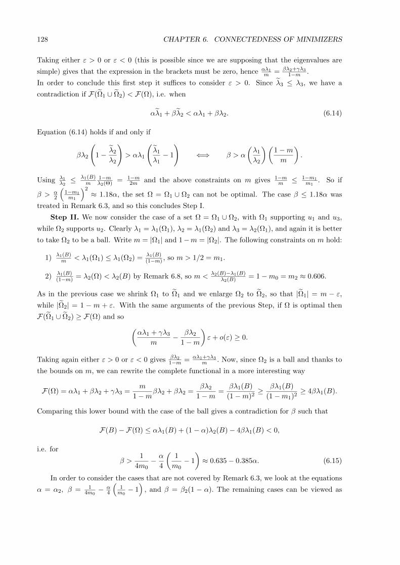
128 CHAPTER 6. CONNECTEDNESS OF MINIMIZERS
Taking either ε > 0 or ε < 0 (this is possible since we are supposing that the eigenvalues are
simple) gives that the expression in the brackets must be zero, hence αλ1m = βλ2+γλ3
1−m .
In order to conclude this first step it suffices to consider ε > 0. Since λ3 ≤ λ3, we have a
contradiction if F(Ω1 ∪ Ω2) < F(Ω), i.e. when
αλ1 + βλ2 < αλ1 + βλ2. (6.14)
Equation (6.14) holds if and only if
βλ2
(1− λ2
λ2
)> αλ1
(λ1
λ1− 1
)⇐⇒ β > α
(λ1
λ2
)(1−mm
).
Using λ1λ2≤ λ1(B)
m1−mλ2(Θ) = 1−m
2m and the above constraints on m gives 1−mm ≤ 1−m1
m1. So if
β > α2
(1−m1m1
)2≈ 1.18α, the set Ω = Ω1 ∪ Ω2 can not be optimal. The case β ≤ 1.18α was
treated in Remark 6.3, and so this concludes Step I.
Step II. We now consider the case of a set Ω = Ω1 ∪ Ω2, with Ω1 supporting u1 and u3,
while Ω2 supports u2. Clearly λ1 = λ1(Ω1), λ2 = λ1(Ω2) and λ3 = λ2(Ω1), and again it is better
to take Ω2 to be a ball. Write m = |Ω1| and 1−m = |Ω2|. The following constraints on m hold:
1) λ1(B)m < λ1(Ω1) ≤ λ1(Ω2) = λ1(B)
(1−m) , so m > 1/2 = m1.
2) λ1(B)(1−m) = λ2(Ω) < λ2(B) by Remark 6.8, so m < λ2(B)−λ1(B)
λ2(B) = 1−m0 = m2 ≈ 0.606.
As in the previous case we shrink Ω1 to Ω1 and we enlarge Ω2 to Ω2, so that |Ω1| = m − ε,while |Ω2| = 1 −m + ε. With the same arguments of the previous Step, if Ω is optimal then
F(Ω1 ∪ Ω2) ≥ F(Ω) and so (αλ1 + γλ3
m− βλ2
1−m
)ε+ o(ε) ≥ 0.
Taking again either ε > 0 or ε < 0 gives βλ2
1−m = αλ1+γλ3
m . Now, since Ω2 is a ball and thanks to
the bounds on m, we can rewrite the complete functional in a more interesting way
F(Ω) = αλ1 + βλ2 + γλ3 =m
1−mβλ2 + βλ2 =
βλ2
1−m=
βλ1(B)
(1−m)2≥ βλ1(B)
(1−m1)2≥ 4βλ1(B).
Comparing this lower bound with the case of the ball gives a contradiction for β such that
F(B)−F(Ω) ≤ αλ1(B) + (1− α)λ2(B)− 4βλ1(B) < 0,
i.e. for
β >1
4m0− α
4
(1
m0− 1
)≈ 0.635− 0.385α. (6.15)
In order to consider the cases that are not covered by Remark 6.3, we look at the equations
α = α2, β = 14m0− α
4
(1m0− 1), and β = β2(1 − α). The remaining cases can be viewed as
6.5. THE TWO DIMENSIONAL CASE 129
0
1
1
A
B
C
α
β
Figure 6.4: The small triangle in the α-β plane
inside a small triangle in the α-β plane, with vertices approximately given by A = (0.275; 0.529),
B = (0.350; 0.500) and C = (0.350; 0.474) (See Figure 6.4).
For these remaining points, it is possible to show that a ball is better than Ω, i.e. that
F(B)− F(Ω) < 0. In fact, the following relations hold between the eigenvalues of the ball and
those of Ω (using m ∈ (m1,m2), the Faber-Krahn and the Krahn-Szego inequalities):
λ1(B)− λ1 ≤(
1− 1
m
)λ1(B) ≤
(1− 1
m2
)λ1(B),
λ2(B)− λ2 = λ2(B)− λ1(B)
1−m≤ λ2(B)− 2λ1(B),
λ3(B)− λ3 ≤ λ2(B)− 2λ1(B)
m≤ λ2(B)− 2λ1(B)
m2.
(6.16)
From (6.16) we get
F(B)−F(Ω) ≤ αλ1(B)
(1− 1
m2
)+ β (λ2(B)− 2λ1(B)) + (1− α− β)
(λ2(B)− 2λ1(B)
m2
).
Hence the ball is better than Ω if
β <2λ1(B)−m2λ2(B)
2λ1(B)− 2m2λ1(B)+ α
(−λ1(B) +m2(λ2(B)− λ1(B)))
2λ1(B)− 2m2λ1(B)≈ 0.58− 0.08α.
This inequality together with (6.15) concludes Step II.
Step III. We now consider the case of a set Ω = Ω1 ∪ Ω2, with Ω1 supporting u1 and u2,
while Ω2 supports u3. Clearly λ1 = λ1(Ω1), λ2 = λ2(Ω1) and λ3 = λ1(Ω2), and it is better to
take Ω2 to be a ball. Let m = |Ω1| and 1−m = |Ω2|. Note that if λ3(Ω) = λ1(Ω2) ≥ mλ3(Ω1),
then Ω can not be optimal. In fact in this case it is better to take the connected set obtained by
130 CHAPTER 6. CONNECTEDNESS OF MINIMIZERS
enlarging Ω1 till unit measure, since this lowers both λ1 and λ2 (by monotonicity), while also
the third eigenvalue is lower, by hypothesis. The following constraints on m hold:
1) λ2(B) > λ2(Ω) = λ2(Ω1) ≥ 2λ1(B)m (see Remark 6.8), so m > 2m0 = m1 ≈ 0.788.
2) In order to have Ω optimal, an upper bound on m follows from inequality mλ3(Ω1) >
λ1(Ω2) explained above and from the fact that λ2(Ω) < λ2(B) (see Remark 6.8). Using
also (2.12) from Theorem 2.11 gives
λ1(B)
(1−m)= λ1(Ω2) < mλ3(Ω1) ≤ mλ2(B)
λ1(B)λ2(Ω1) < m
λ2(B)2
λ1(B).
This means m2 −m+m20 < 0, which gives the upper bound
m <λ2(B) +
√λ2(B)2 − 4λ1(B)2
2λ2(B)= m2 ≈ 0.808.
As in the previous steps we can enlarge Ω1 to Ω1 and we can shrink Ω2 to Ω2, in order that
|Ω1| = m+ ε, while |Ω2| = 1−m− ε. The following ratios between the eigenvalues of Ω1 ∪ Ω2
and those of Ω hold (for ε << 1) :
λ1
λ1=λ2
λ2=
m
m+ ε≈ 1− ε
m;
λ3
λ3=
1−m1−m− ε
≈ 1 +ε
1−m.
In order to be optimal, Ω must satisfy
αλ1 + βλ2 + (1− α− β)λ3 ≥ αλ1 + βλ2 + (1− α− β)λ3.
An analogous argument to that in Step I and Step II gives a contradiction for β & 0.914−0.948α.
Actually we can obtain a better result observing that Ω is worse than Ω1 enlarged to unit measure
(which we will call Ω in the following) if β is suitably large. We denote by λi the eigenvalues
of Ω and we again write γ = 1−α−β for the sake of simplicity. The following relations between
the eigenvalues hold: λ1 = mλ1, λ2 = mλ2 and λ3 = mλ3(Ω1) ≤ mm0λ2, using (2.12) from
Theorem 2.11 by Ashbaugh and Benguria. This gives
F(Ω) = αλ1 + βλ2 + γλ3 ≤ F(Ω) + α(m− 1)λ1 + β(m− 1)λ2 + γ
(m
m1− 1
)λ2.
Clearly Ω can not be optimal when F(Ω)−F(Ω) < 0, which holds if
α(m− 1)λ1 +
[β(m− 1) + γ
(m
m0− 1
)]λ2 < 0.
The first part (2.11) of Theorem 2.11 gives that the result follows if[α(m− 1)m0 + β(m− 1) + γ
(m
m0− 1
)]λ2 < 0.
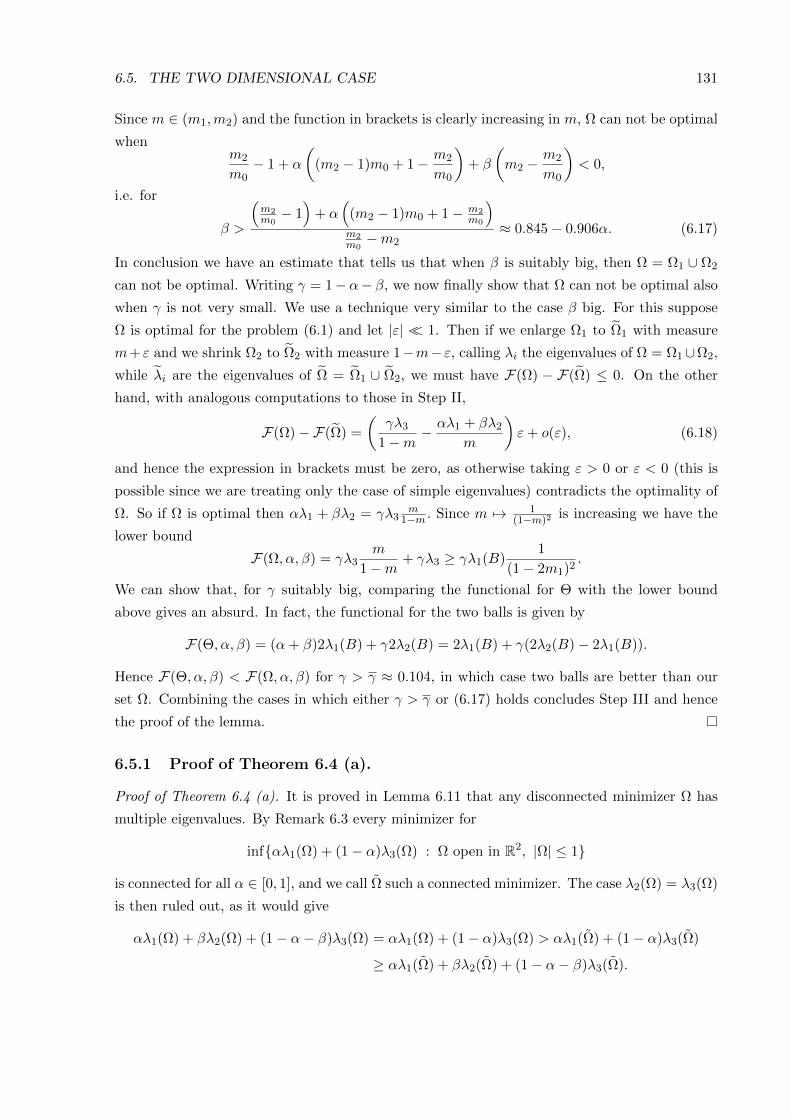
6.5. THE TWO DIMENSIONAL CASE 131
Since m ∈ (m1,m2) and the function in brackets is clearly increasing in m, Ω can not be optimal
whenm2
m0− 1 + α
((m2 − 1)m0 + 1− m2
m0
)+ β
(m2 −
m2
m0
)< 0,
i.e. for
β >
(m2m0− 1)
+ α(
(m2 − 1)m0 + 1− m2m0
)m2m0−m2
≈ 0.845− 0.906α. (6.17)
In conclusion we have an estimate that tells us that when β is suitably big, then Ω = Ω1 ∪ Ω2
can not be optimal. Writing γ = 1−α− β, we now finally show that Ω can not be optimal also
when γ is not very small. We use a technique very similar to the case β big. For this suppose
Ω is optimal for the problem (6.1) and let |ε| << 1. Then if we enlarge Ω1 to Ω1 with measure
m+ ε and we shrink Ω2 to Ω2 with measure 1−m− ε, calling λi the eigenvalues of Ω = Ω1∪Ω2,
while λi are the eigenvalues of Ω = Ω1 ∪ Ω2, we must have F(Ω) − F(Ω) ≤ 0. On the other
hand, with analogous computations to those in Step II,
F(Ω)−F(Ω) =
(γλ3
1−m− αλ1 + βλ2
m
)ε+ o(ε), (6.18)
and hence the expression in brackets must be zero, as otherwise taking ε > 0 or ε < 0 (this is
possible since we are treating only the case of simple eigenvalues) contradicts the optimality of
Ω. So if Ω is optimal then αλ1 + βλ2 = γλ3m
1−m . Since m 7→ 1(1−m)2 is increasing we have the
lower bound
F(Ω, α, β) = γλ3m
1−m+ γλ3 ≥ γλ1(B)
1
(1− 2m1)2.
We can show that, for γ suitably big, comparing the functional for Θ with the lower bound
above gives an absurd. In fact, the functional for the two balls is given by
F(Θ, α, β) = (α+ β)2λ1(B) + γ2λ2(B) = 2λ1(B) + γ(2λ2(B)− 2λ1(B)).
Hence F(Θ, α, β) < F(Ω, α, β) for γ > γ ≈ 0.104, in which case two balls are better than our
set Ω. Combining the cases in which either γ > γ or (6.17) holds concludes Step III and hence
the proof of the lemma.
6.5.1 Proof of Theorem 6.4 (a).
Proof of Theorem 6.4 (a). It is proved in Lemma 6.11 that any disconnected minimizer Ω has
multiple eigenvalues. By Remark 6.3 every minimizer for
infαλ1(Ω) + (1− α)λ3(Ω) : Ω open in R2, |Ω| ≤ 1
is connected for all α ∈ [0, 1], and we call Ω such a connected minimizer. The case λ2(Ω) = λ3(Ω)
is then ruled out, as it would give
αλ1(Ω) + βλ2(Ω) + (1− α− β)λ3(Ω) = αλ1(Ω) + (1− α)λ3(Ω) > αλ1(Ω) + (1− α)λ3(Ω)
≥ αλ1(Ω) + βλ2(Ω) + (1− α− β)λ3(Ω).
132 CHAPTER 6. CONNECTEDNESS OF MINIMIZERS
Therefore any disconnected minimizer must satisfy λ1(Ω) = λ2(Ω) and can be viewed as the
union of a disk supporting the first eigenvalue with a connected set supporting the second and
third, since a minimizer with three connected components was ruled out by Lemma 6.10.
6.5.2 Proof of Theorem 6.4 (b).
Proof of Theorem 6.4 (b). Let α + β < 1, and let Ω be a connected minimizer for inf(α +
β)λ2(Ω)+(1−α−β)λ3(Ω) : Ω open in R2, |Ω| ≤ 1, while there are no disconnected minimizers
by hypothesis. Theorem 6.4 (a) then gives λ1(Ω) = λ2(Ω) for a disconnected minimizer Ω for
problem (6.1), whereby
αλ1(Ω) + βλ2(Ω)+(1− α− β)λ3(Ω) = (α+ β)λ2(Ω) + (1− α− β)λ3(Ω)
> (α+ β)λ2(Ω) + (1− α− β)λ3(Ω),
≥ αλ1(Ω) + βλ2(Ω) + (1− α− β)λ3(Ω),
which contradicts the minimality of Ω and thus the proof is concluded.
Bibliography
The thesis is based on the following papers
[M1] D. Bucur, D. Mazzoleni, A. Pratelli, B. Velichkov, Lipschitz regularity of the eigenfunc-
tions on optimal domains, to appear on Arch. Rational Mech. Anal., preprint available at
http://cvgmt.sns.it/person/977/.
[M2] M. Iversen, D. Mazzoleni, Minimising convex combinations of low eigenvalues,
ESAIM:COCV, 20 (2) 442–459 (2014).
[M3] D. Mazzoleni, Boundedness of minimizers for spectral problems in RN , to appear on Rend.
Sem. Mat. Univ. Padova, preprint available at http://cvgmt.sns.it/person/977/.
[M4] D. Mazzoleni, A. Pratelli, Existence of minimizers for spectral problems, J. Math. Pures
Appl. 100 (3) (2013), 433-453.
Other references
[1] M. Abramowitz, I.A. Stegun, eds. Handbook of Mathematical Functions with Formulas,
Graphs, and Mathematical Tables, Dover Publications, New York (1972).
[2] H.W. Alt, L.A. Caffarelli, Existence and regularity for a minimum problem with free
boundary, J. Reine Angew. Math., 325 (1981), 105–144.
[3] H.W. Alt, L.A. Caffarelli, A. Friedman, Variational problems with two phases and their
free boundaries, Trans. Amer. Math. Soc., 282 (1984), 431–461.
[4] P. Antunes, P. Freitas, Numerical optimization of low eigenvalues of the Dirichlet and
Neumann Laplacians, J. Optim. Theory Appl., 154 (1) (2012), 235–257.
[5] M.S. Ashbaugh, Open problems on eigenvalues of the Laplacian, In Analytic and Geometric
Inequalities and Applications, Math. Appl. 478, Kluwer Acad. Publ., Dordrecht (1999),
13–28.
133
134 BIBLIOGRAPHY
[6] M.S. Ashbaugh, The universal eigenvalue bounds of Payne-Polya-Weinberger, Hile-
Protter, and H C Yang, Proc. Indian Acad. Sci. (Math. Sci.), 112 (1) (2002), 3–30.
[7] M.S. Ashbaugh, R. Benguria, Proof of the Payne-Polya-Weinberger conjecture, Bull.
Amer. Math. Soc., 25 (1) (1991), 19–29.
[8] M. S. Ashbaugh, R. Benguria, Isoperimetric bound for λ3/λ2 for the membrane problem,
Duke Math. J., 63 (1991), 333–341.
[9] M. van den Berg, On Rayleigh’s formula for the first Dirichlet eigenvalue of a radial
perturbation of a ball, J. Geom. Anal., 23 (3) (2013), 1427–1440.
[10] M. van den Berg, M. Iversen, On the minimization of Dirichlet eigenvalues of the Laplace
operator, J. Geom. Anal., 23 (2) (2013), 660–676.
[11] A. Berger, E. Oudet, The eigenvalues of the Laplacian with Dirichlet boundary conditions
in R2 are almost never minimized by disks, in preparation.
[12] L. Brasco, C. Nitsch, A. Pratelli, On the boundary of the attainable set of the Dirichlet
spectrum, Z. Angew. Math. Phys., 64 (3) (2013), 591–597.
[13] T. Briancon, J. Lamboley, Regularity of the optimal shape for the first eigenvalue of the
Laplacian with volume and inclusion constraints, Ann. I. H. Poincare – AN, 26 (4) (2009),
1149–1163.
[14] T. Briancon, M. Hayouni, M. Pierre, Lipschitz continuity of state functions in some optimal
shaping, Calc. Var. PDE, 23 (1) (2005), 13–32.
[15] D. Bucur, How to prove existence in shape optimization, Control and cybernetics, 34 (1)
(2005), 103–116.
[16] D. Bucur, Minimization of the k-th eigenvalue of the Dirichlet Laplacian, Arch. Rational
Mech. Anal., 206 (3) (2012), 1073–1083.
[17] D. Bucur, Regularity of optimal convex shapes, J. Convex Anal., 10 (2003), 501–516.
[18] D. Bucur, Uniform concentration-compactness for Sobolev spaces on variable domains, J.
Diff. Eq., 162 (2000), 427–450.
[19] D. Bucur, G. Buttazzo, On the characterization of the compact embedding of Sobolev
spaces, Calc. Var. PDE, 44 (3-4) (2012), 455–475.
[20] D. Bucur, G. Buttazzo, Variational Methods in Shape Optimization Problems. Progress in
Nonlinear Differential Equations 65, Birkhauser Verlag, Basel (2005).
BIBLIOGRAPHY 135
[21] D. Bucur, G. Buttazzo, I. Figueiredo, On the attainable eigenvalues of the Laplace oper-
ator, SIAM J. Math. Anal., 30 (3) (1999), 527–536.
[22] D. Bucur, G. Buttazzo, B. Velichkov, Spectral optimization problems with internal con-
straint, Ann. I. H. Poincare – AN 30 (3) (2013), 477–495.
[23] D. Bucur, A. Henrot, Minimization of the third eigenvalue of the Dirichlet Laplacian, Proc.
Roy. Soc. London, 456 (2000), 985–996.
[24] G. Buttazzo, Spectral optimization problems, Rev. Mat. Complut., 24 (2) (2011), 277–322.
[25] G. Buttazzo, G. Dal Maso, Shape optimization for Dirichlet problems: relaxed formulation
and optimality conditions, Appl. Math. Optim., 23 (1991), 17–49.
[26] G. Buttazzo, G. Dal Maso, An existence result for a class of shape optimization problems,
Arch. Rational Mech. Anal., 122 (2) (1993), 183–195.
[27] L. Caffarelli, D. Jerison, C. Kenig, Some new monotonicity theorems with applications to
free boundary problems, Annals of Mathematics, 155 (2) (2002), 369–404.
[28] D. Cioranescu, F. Murat, A strange term coming from nowhere, Topics in the Mathemat-
ical Modelling of Composite Materials, Progress in Nonlinear Differential Equations and
Their Applications, 31 (1997), 45–93.
[29] R. Courant, D. Hilbert, Methods of Mathematical Physics, voll. 1 and 2, Wiley, New York
(1953 and 1962).
[30] G. Dal Maso, An Introduction to Γ-convergence. Birkhauser, Boston (1993).
[31] G. Dal Maso, U. Mosco, Wiener criteria and energy decay for relaxed Dirichlet problems,
Arch. Rational Mech. Anal., 95 (4) (1986), 345–387.
[32] G. Dal Maso, U. Mosco, Wiener’s criterion and Γ-convergence, Appl. Math. Optim., 15
(1987), 15–63.
[33] E. Davies, Heat kernels and spectral theory. Cambridge University Press, 1989.
[34] G. De Philippis, B. Velichkov, Existence and regularity of minimizers for some spectral
optimization problems with perimeter constraint, Appl. Math. Optim., 69 (2014), 199–231.
[35] G. Faber, Beweiss, dass unter alles homogenen Membranen von gleicher Flache und gleicher
Spannung die kreisformige den tiefsten Grundton gibt, Sitz. Ber. Bayer. Akad. Wiss.
(1923), 169–172.
[36] D. Gilbarg, N. Trudinger, Elliptic partial differential equations of second order, Springer,
second edition (2001).
136 BIBLIOGRAPHY
[37] A. Henrot, Minimization problems for eigenvalues of the Laplacian, J. Evol. Equ., 3 (3)
(2003), 443–461.
[38] A. Henrot, Extremum Problems for Eigenvalues of Elliptic Operators. Frontiers in Math-
ematics, Birkhauser Verlag, Basel (2006).
[39] A. Henrot, M. Pierre, Variation et Optimisation de Formes. Une Analyse Geometrique.
Mathematiques & Applications 48, Springer-Verlag, Berlin (2005).
[40] I. Hong, On an inequality concerning the eigenvalue problem of membrane, Kodai Math.
Sem. Rep., (1954), 113–114.
[41] C.-Y. Kao, B. Osting, Minimal convex combinations of three sequential Laplace-Dirichlet
eigenvalues, Appl. Math. Optim., 69 (2014), 123–139.
[42] S. Kesavan, Topics in functional analysis and applications, Wiley Eastern Limited (1989).
[43] E. Krahn, Uber eine von Rayleigh formulierte Minimaleigenschaft des Kreises, Math. Ann.,
bf 94 (1924), 97–100.
[44] E. Krahn, Uber Minimaleigenschaften der Kugel in drei und mehr Dimensionen, Acta
Comm. Univ. Dorpat., A9 (1926), 1–44.
[45] P.L. Lions, The concentration-compactness principle in the calculus of variations. The
locally compact case, part 1, Ann. I. H. Poincare – AN, 1 (2) (1984), 109–145.
[46] E. Oudet, Numerical minimization of eigenmodes of a membrane with respect to the
domain, ESAIM:COCV, 10 (3) (2004), 315–330.
[47] L.E. Payne, G. Polya, H.F. Weinberger, On the ratio of consecutive eigenvalues, J. Math.
Phys., 35 (1956), 289–298.
[48] L. Rayleigh, The Theory of Sound, 1st edition, Macmillan, London (1877).
[49] G. Szego, Inequalities for certain eigenvalues of a membrane of given area, J. Rational
Mech. Anal., 3 (1954), 343–356.
[50] G. Talenti, Elliptic equations and rearrangements, Ann. Scuola Norm. Sup. Pisa Cl. Sci.,
3 (4), 697–718.
[51] B. Velichkov, Existence and regularity results for some shape optimization problems, Ph.D.
Thesis, Scuola Normale Superiore (Pisa) and Universite J. Fourier (Grenoble), 2013.
[52] S. A. Wolf, Asymptotic and Numerical Analysis of Linear and Nonlinear Eigenvalue Prob-
lems, Ph.D. Thesis, Stanford University (1993).
BIBLIOGRAPHY 137
[53] S. A. Wolf, J. B. Keller, Range of the First Two Eigenvalues of the Laplacian, Proc. R.
Soc. Lond. A, 447, (1930) (1994), 397–412.
[54] W.P. Ziemer, Weakly Differentiable Functions. Springer-Verlag, Berlin (1989).