Exercise Sheet 1...Machine Learning Nando de Freitas January 22, 2015 2Rn nis diagonal with positive...

Machine LearningNando de FreitasJanuary 22, 2015

Exercise Sheet 1

1 Probability revision 1: Student-t as an infinite mixture ofGaussians

Show that an infinite mixture of Gaussian distributions, with Gamma distributions as mixingweights in the following manner:

p(x) =

∫ ∞0N (x|0, 1/λ)Ga(λ|ν/2, ν/2)dλ (1)

is equal to a t-distribution:

p(x) = (2πν

2)−

12

Γ(ν+12 )

Γ(ν/2)(1 +

x2

ν)−

ν+12 = T (x|0, 1, ν) (2)

I recommend that you look at section 2.4.2 of Kevin’s book for visualization of these distribu-tions. You can also look them up in Wikipedia. Hint: Consider a change of variable z = λ∆.

This popular integration trick appears in the formulation of numerous statistical and neu-roscience models, for example:

• Martin Wainwright and Eero Simoncelli. “Scale mixtures of Gaussians and the statisticsof natural images.” NIPS. 1999.

• Gavin Cawley, Nicola Talbot, and Mark Girolami. “Sparse multinomial logistic regressionvia Bayesian L1 regularisation.” NIPS. 2007.

2 Reducing the cost of linear regression for large d small n

The ridge method is a regularized version of least squares, with objective function:

minθ∈Rd

‖y −Xθ‖22 + δ2‖θ‖22.

Here, δ is a scalar, the input matrix X ∈ Rn×d and the output vector y ∈ Rn. The param-eter vector θ ∈ Rd is obtained by differentiating the above cost function, yielding the normalequations

(XTX + δ2Id)θ = XTy,

where Id is the d×d identity matrix. The predictions y = y(X?) for new test points X? ∈ Rn?×dare obtained by evaluating the hyperplane

y = X?θ = X?(XTX + δ2Id)

−1XTy = Hy. (3)

The matrix H is known as the hat matrix because it puts a “hat” on y.


1. Show that the solution can be written as θ = XTα, where α = δ−2(y −Xθ).

2. Show that α can also be written as follows: α = (XXT + δ2In)−1y and, hence, thepredictions can be written as follows:

y = X?θ = X?XTα = [X?X

T ]([XXT ] + δ2In)−1y (4)

(This is an awesome trick because if n = 20 patients with d = 10, 000 gene measurements,the computation of α only requires inverting the n×nmatrix, while the direct computationof θ would have required the inversion of a d× d matrix.)

3 Linear algebra revision: Eigen-decompositions

Once you start looking at raw data, one of the first things you notice is how redundant itoften is. In images, it’s often not necessary to keep track of the exact value of every pixel; intext, you don’t always need the counts of every word. Correlations among variables also createredundancy. For example, if every time a gene, say A, is expressed another gene B is alsoexpressed, then to build a tool that predicts patient recovery rate from gene expression data, itseems reasonable to remove either A or B. Most situations are not as clear-cut.

In this question, we’ll look at eigenvalue methods for factoring and projecting data matrices(images, document collections, image collections), with an eye to one of the most common uses:Converting a high-dimensional data matrix to a lower-dimensional one, while minimizing theloss of information.

The Singular Value Decomposition (SVD) is a matrix factorization that has many applica-tions in information retrieval, collaborative filtering, least-squares problems and image process-ing.

Let X be an n × n matrix of real numbers; that is X ∈ Rn×n. Assume that X has neigenvalue-eigenvector pairs (λi,qi):

Xqi = λiqi i = 1, . . . , n

If we place the eigenvalues λi ∈ R into a diagonal matrix Λ and gather the eigenvectors qi ∈ Rninto a matrix Q, then the eigenvalue decomposition of X is given by

X[

q1 q2 . . . qn]

=[

q1 q2 . . . qn]σ1

σ2. . .

σn

(5)

or, equivalently,X = QΛQ−1.

For a symmetric matrix, i.e. X = XT , one can show that X = QΛQT . But what if X is nota square matrix? Then the SVD comes to the rescue. Given X ∈ Rm×n, the SVD of X is afactorization of the form

X = UΣVT .

These matrices have some interesting properties:


• Σ ∈ Rn×n is diagonal with positive entries (singular values σ in the diagonal).

• U ∈ Rm×n has orthonormal columns: uTi uj = 1 only when i = j and 0 otherwise.

• V ∈ Rn×n has orthonormal columns and rows. That is, V is an orthogonal matrix, soV−1 = VT .

Often, U is m-by-m, not m-by-n. The extra columns are added by a process of orthogonal-ization. To ensure that dimensions still match, a block of zeros is added to Σ. For our purposes,however, we will only consider the version where U is m-by-n, which is known as the thin-SVD.

It will turn out useful to introduce the vector notation:

Xvj = σjuj j = 1, 2, . . . , n

where u ∈ Rm are the left singular vectors, σ ∈ [0,∞) are the singular values and v ∈ Rn arethe right singular vectors. That is,

X[

v1 v2 . . . vn]

=[

u1 u2 . . . un]σ1

σ2. . .

σn

(6)

or XV = UΣ. Note that there is no assumption that m ≥ n or that X has full rank. Inaddition, all diagonal elements of Σ are non-negative and in non-increasing order:

σ1 ≥ σ2 ≥ . . . ≥ σp ≥ 0

where p = min (m,n).

Question: Outline a procedure for computing the SVD of a matrix X. Hint: assume you canfind the eigenvalue decompositions of the symmetric matrices XTX and XXT .

4 Representing data with eigen-decompositions

It is instructive to think of the SVD as a sum of rank-one matrices:

Xr =r∑j=1

σjujvTj ,

with r ≤ min(m,n). What is so useful about this expansion is that the k − th partial sumcaptures as much of the “energy” of X as possible. In this case, “energy” is defined by the2-norm of a matrix :

‖X‖2 = σ1,


which can also be written as follows:

‖X‖2 = max‖y‖2=1

‖Xy‖2,

This definition of the norm of a matrix builds upon our standard definition for the 2-norm ofa vector ‖y‖2 =

√yTy. Essensiatily, you can think of the norm of a matrix as how much it

expands the unit-circle ‖y‖2 = 1, when applied to it.

Question: Using the SVD, prove that the two definitions of the 2-norm of a matrix areequivalent.

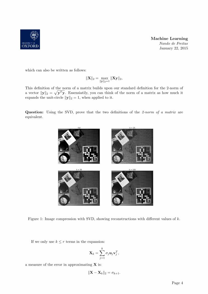
full k = 25

k = 50 k = 100

Figure 1: Image compression with SVD, showing reconstructions with different values of k.

If we only use k ≤ r terms in the expansion:

Xk =

k∑j=1

σjujvTj ,

a measure of the error in approximating X is:

‖X−Xk‖2 = σk+1.


We will illustrate the value of this with an image compression example. Figure 1 shows theoriginal image X, and three SVD compressions Xk. We can see that when k is low, we get acoarse version of the image. As more eigen-components are added, we get more high-frequencydetails – text becomes legible and pieces of the go game become circular instead of blocky.

The memory savings are dramatic as we only need to store the eigenvalues and eigen-vectorsup to order k in order to generate the compressed image Xk. Too see this, let the original imagebe of size 961 pixels by 1143 pixels, stored as a 961-by-1143 array of 32-bit floats. The total sizeof the data is over 17 MB (the number of entries in the array times 4 bytes per entry). UsingSVD, we can compress and display the image to obtain the following numbers:

compression bytes reduction

original 17 574 768 0%k = 100 842 000 95.2%k = 50 ? 97.6%k = 25 ? 98.8%

Question: Replace the question marks in the tables above with actual numbers of bytes.

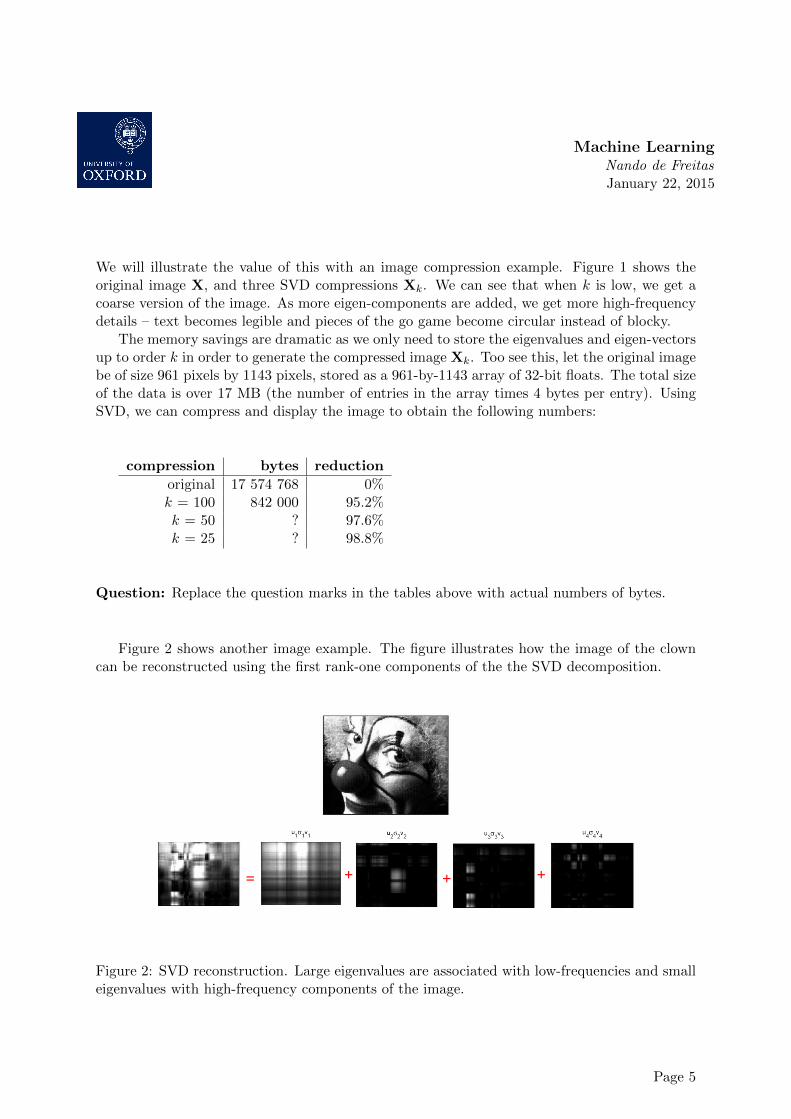
Figure 2 shows another image example. The figure illustrates how the image of the clowncan be reconstructed using the first rank-one components of the the SVD decomposition.

++ += ++ +=

Figure 2: SVD reconstruction. Large eigenvalues are associated with low-frequencies and smalleigenvalues with high-frequency components of the image.

Exercise Sheet 1...Machine Learning Nando de Freitas January 22, 2015 2Rn nis diagonal with positive...

Documents

Transcript of Exercise Sheet 1...Machine Learning Nando de Freitas January 22, 2015 2Rn nis diagonal with positive...