EXAFS Analysis - X-ray Absorption

EXAFS Analysis

Matthew Newville

Center for Advanced Radiation SourcesThe University of Chicago

9-July-2013

http://xafs.org/Workshops/IIT2013

EXAFS Analysis with feff and ifeffit M Newville Univ of Chicago 9-July-2013 http://xafs.org/Workshops/IIT2013

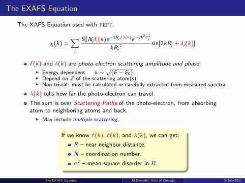
The EXAFS Equation

The XAFS Equation used with feff:

χ(k) =∑j

S20 Nj fj(k)e−2Rj/λ(k)e−2k2σ2

j

kRj2 sin[2kRj + δj(k)]

f (k) and δ(k) are photo-electron scattering amplitude and phase:I Energy dependent k ∼

√(E − E0).

I Depend on Z of the scattering atom(s).I Non-trivial: must be calculated or carefully extracted from measured spectra.

λ(k) tells how far the photo-electron can travel.

The sum is over Scattering Paths of the photo-electron, from absorbingatom to neighboring atoms and back.

I May include multiple scattering.

If we know f (k), δ(k), and λ(k), we can get:

R – near neighbor distance.

N – coordination number.

σ2 – mean-square disorder in R.

The EXAFS Equation M Newville Univ of Chicago 9-July-2013

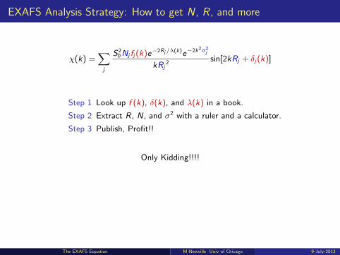
EXAFS Analysis Strategy: How to get N , R , and more

χ(k) =∑j


j


Step 1 Look up f (k), δ(k), and λ(k) in a book.

Step 2 Extract R, N, and σ2 with a ruler and a calculator.

Step 3 Publish, Profit!!

Only Kidding!!!!


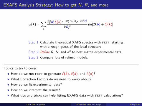
EXAFS Analysis Strategy: How to get N , R , and more

χ(k) =∑j


j


Step 1 Calculate theoretical XAFS spectra with feff, startingwith a rough guess of the local structure.

Step 2 Refine R, N, and σ2 to best match experimental data.

Step 3 Compare lots of refined models.

Topics to try to cover:

How do we run feff to generate f (k), δ(k), and λ(k)?

What Correction Factors do we need to worry about?

How do we fit experimental data?

How do we interpret the results?

What tips and tricks can help fitting EXAFS data with feff calculations?


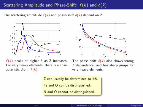
Scattering Amplitude and Phase-Shift: f (k) and δ(k)

The scattering amplitude f (k) and phase-shift δ(k) depend on Z:

f (k) peaks at higher k as Z increases.For very heavy elements, there is a char-acteristic dip in f (k).

The phase shift δ(k) also shows strongZ dependence, and has sharp jumps forvery heavy elements.

Z can usually be determined to ±5.

Fe and O can be distinguished.

N and O cannot be distinguished.

feff M Newville Univ of Chicago 9-July-2013

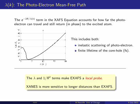
λ(k): The Photo-Electron Mean-Free Path

The e−2R/λ(k) term in the XAFS Equation accounts for how far the photo-electron can travel and still return (in phase) to the excited atom.

This includes both:

inelastic scattering of photo-electron.

finite lifetime of the core-hole (fs).

The λ and 1/R2 terms make EXAFS a local probe.

XANES is more sensitive to longer distances than EXAFS.


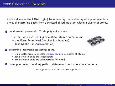
feff Calculation Overview

feff calculates the EXAFS χ(k) by simulating the scattering of a photo-electronalong all scattering paths from a selected absorbing atom within a cluster of atoms.

1 build atomic potentials. To simplify calculations,

Use the Cup-Cake Tin Approximation: atomic potentials upto a uniform Fermi level (no chemical bonding).

(aka Muffin-Tin Approximation)

2 determine important scattering paths.

I Build paths from a selected central atom in a cluster of atomsI decide which ones are “degenerate” .I decide which ones are unimportant for XAFS

3 move photo-electron along path to determine f and δ as a function of k:

propagate ⇒ scatter ⇒ propagate ⇒ . . . .


feff: what’s so hard about that??

feff includes sophisticated techniques to calculate of f (k), δ(k), and λ(k).

Curved Wave Effects the photo-electron goes out as spherical wave andscatters from atoms with finite size.

Muffin-Tin Approximation: Makes the calculations tractable, but is anapproximation.

Multiple Scattering the photo-electron can scatter multiple times. Mostimportant at low k and for linear paths.

Extrinsic Losses λ(k): self-energy and core-hole lifetime.

Intrinsic Losses S20 : the absorbing atom relaxes to the presence of the hole

left in the core electron level.

Polarization Effects synchrotron beams are highly polarized, which needs tobe taken into account. This is simple for K edges (s → p isdipole), but slightly more complicated for L and M edges.

Usually, you don’t have to worry about these things!


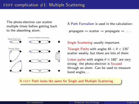
feff complication #1: Multiple Scattering

The photo-electron can scattermultiple times before getting backto the absorbing atom:

Single Scattering

Triangle Paths

Focused Multiple Scattering

A Path Formalism is used in the calculation:

propagate ⇒ scatter ⇒ propagate ⇒ . . . .

Single Scattering usually important.

Triangle Paths with angles 45 < θ < 135◦

scatter weakly, but there are lots of them.

Linear paths with angles θ ≈ 180◦ are verystrong: the photo-electron is focusedthrough an atom. Can be used to measurebond angles. . .

A feff Path looks the same for Single and Multiple Scattering

feff complications M Newville Univ of Chicago 9-July-2013

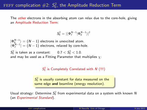
feff complication #2: S20 , the Amplitude Reduction Term

The other electrons in the absorbing atom can relax due to the core-hole, givingan Amplitude Reduction Term:

S20 = |〈ΦN−1

f |ΦN−10 〉|2

|ΦN−10 〉 = (N − 1) electrons in unexcited atom.〈ΦN−1

f | = (N − 1) electrons, relaxed by core-hole.

S20 is taken as a constant: 0.7 < S2

0 < 1.0.and may be used as a Fitting Parameter that multiplies χ:

S20 is Completely Correlated with N (!!!)

S20 is usually constant for data measured on the

same edge and beamline (energy resolution).

Usual strategy: Determine S20 from experimental data on a system with known N

(an Experimental Standard).

feff complications M Newville Univ of Chicago 9-July-2013

Practical feff

Good News: you don’t have to worry about the hard parts (mostly)!

The normal scheme for using feff for EXAFS data analysis is:

1 Start with a structure close to the local atomic structure of your sample, andgenerate x,y,z coordinates for the atoms. Often a crystal structure is close – it doesnot have to be perfect!

2 Run feff. This creates a feffnnnn.dat files for each path in your structure.

3 Use these Path Files in to model measured XAFS in an analysis program.

artemis and sixpack makes this even easier: they run and manages feff for you.

Having good starting structures can be important, but you do notneed the exact structure to use feff.

You can (may need to) mix structural models to model real data.

Practical FEFF M Newville Univ of Chicago 9-July-2013

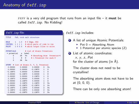
Anatomy of feff.inp

feff is a very old program that runs from an input file – it must becalled feff.inp. No Kidding!

feff.inp file:

TITLE FeO, rock salt structure

HOLE 1 1.0 # K Edge, S02

CONTROL 1 1 1 1 # which parts of code to run

PRINT 1 0 0 3 # which output files to write

POTENTIALS # list of Atomic Potentials

* potential z label

0 26 Fe # Absorbing Atom Potential=0

1 8 O # 1 Potential for each Z

2 26 Fe

ATOMS # list of Atomic X, Y, Z, Potential

0.00000 0.00000 0.00000 0 Fe

0.00000 0.00000 -2.13870 1 O

-2.13870 0.00000 0.00000 1 O

0.00000 -2.13870 0.00000 1 O

0.00000 0.00000 2.13870 1 O

2.13870 0.00000 0.00000 1 O

0.00000 2.13870 0.00000 1 O

0.00000 2.13870 2.13870 2 Fe

0.00000 -2.13870 -2.13870 2 Fe

-2.13870 2.13870 0.00000 2 Fe

2.13870 -2.13870 0.00000 2 Fe

0.00000 -2.13870 2.13870 2 Fe

feff.inp includes:

1 A list of unique Atomic Potentials:I Pot 0 = Absorbing AtomI 1 Potential per atomic species (Z)

2 List of atomic coordinates:x , y , z , Pot

for the cluster of atoms (in A).

The cluster does not need to becrystalline!

The absorbing atom does not have to beat (0, 0, 0).

There can be only one absorbing atom!


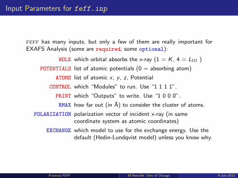
Input Parameters for feff.inp

feff has many inputs, but only a few of them are really important forEXAFS Analysis (some are required, some optional):

HOLE which orbital absorbs the x-ray (1 = K , 4 = LIII )

POTENTIALS list of atomic potentials (0 = absorbing atom)

ATOMS list of atomic x , y , z , Potential

CONTROL which “Modules” to run. Use “1 1 1 1”.

PRINT which “Outputs” to write. Use “1 0 0 0”.

RMAX how far out (in A) to consider the cluster of atoms.

POLARIZATION polarization vector of incident x-ray (in samecoordinate system as atomic coordinates)

EXCHANGE which model to use for the exchange energy. Use thedefault (Hedin-Lundqvist model) unless you know why.


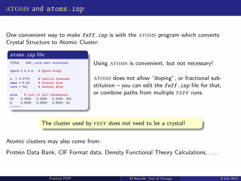
atoms and atoms.inp

One convenient way to make feff.inp is with the atoms program which convertsCrystal Structure to Atomic Cluster:

atoms.inp file:

TITLE FeO, rock salt structure

space f m 3 m # Space Group

a = 4.2774 # Lattice Constant

rmax = 6.00 # Cluster Size

core = Fe1 # Central Atom

atom # List of Cell Parameters

Fe 0.0000 0.0000 0.0000 Fe1

O 0.5000 0.5000 0.5000 O1

------

Using atoms is convenient, but not necessary!

atoms does not allow “doping”, or fractional sub-stitution – you can edit the feff.inp file for that,or combine paths from multiple feff runs.

The cluster used by feff does not need to be a crystal!

Atomic clusters may also come from:

Protein Data Bank, CIF Format data, Density Functional Theory Calculations, . . . .


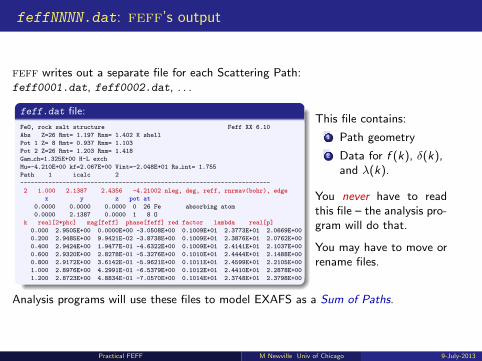
feffNNNN.dat: feff’s output

feff writes out a separate file for each Scattering Path:feff0001.dat, feff0002.dat, . . .

feff.dat file:

FeO, rock salt structure Feff XX 6.10

Abs Z=26 Rmt= 1.197 Rnm= 1.402 K shell

Pot 1 Z= 8 Rmt= 0.937 Rnm= 1.103

Pot 2 Z=26 Rmt= 1.203 Rnm= 1.418

Gam ch=1.325E+00 H-L exch

Mu=-4.210E+00 kf=2.067E+00 Vint=-2.048E+01 Rs int= 1.755

Path 1 icalc 2

-----------------------------------------------------------------------

2 1.000 2.1387 2.4356 -4.21002 nleg, deg, reff, rnrmav(bohr), edge

x y z pot at

0.0000 0.0000 0.0000 0 26 Fe absorbing atom

0.0000 2.1387 0.0000 1 8 O

k real[2*phc] mag[feff] phase[feff] red factor lambda real[p]

0.000 2.9505E+00 0.0000E+00 -3.0508E+00 0.1009E+01 2.3773E+01 2.0669E+00

0.200 2.9485E+00 9.9421E-02 -3.8738E+00 0.1009E+01 2.3876E+01 2.0762E+00

0.400 2.9424E+00 1.9477E-01 -4.6322E+00 0.1009E+01 2.4141E+01 2.1037E+00

0.600 2.9320E+00 2.8278E-01 -5.3276E+00 0.1010E+01 2.4444E+01 2.1488E+00

0.800 2.9172E+00 3.6142E-01 -5.9621E+00 0.1011E+01 2.4599E+01 2.2105E+00

1.000 2.8976E+00 4.2991E-01 -6.5379E+00 0.1012E+01 2.4410E+01 2.2878E+00

1.200 2.8723E+00 4.8834E-01 -7.0570E+00 0.1014E+01 2.3748E+01 2.3798E+00

This file contains:

1 Path geometry

2 Data for f (k), δ(k),and λ(k).

You never have to readthis file – the analysis pro-gram will do that.

You may have to move orrename files.

Analysis programs will use these files to model EXAFS as a Sum of Paths.


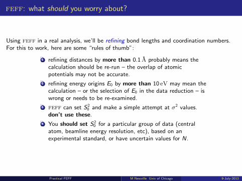
feff: what should you worry about?

Using feff in a real analysis, we’ll be refining bond lengths and coordination numbers.For this to work, here are some “rules of thumb”:

1 refining distances by more than 0.1 A probably means thecalculation should be re-run – the overlap of atomicpotentials may not be accurate.

2 refining energy origins E0 by more than 10 eV may mean thecalculation – or the selection of E0 in the data reduction – iswrong or needs to be re-examined.

3 feff can set S20 and make a simple attempt at σ2 values.

don’t use these.

4 You should set S20 for a particular group of data (central

atom, beamline energy resolution, etc), based on anexperimental standard, or have uncertain values for N.


Structural Disorder and the Pair Distribution Function

An EXAFS measurement averages billions of snapshots of the local structure:

Each absorbed x-ray generates 1 photo-electron.

the photo-electron / core-hole pair lives for about 10−15 s –much faster than the thermal vibrations (10−12 s).

An EXAFS measurement samples 104 (dilute fluorescence)to 1010 absorbed x-rays for each energy point.

So far, we’ve put this in the EXAFS Equation as χ ∼ N exp(−2k2σ2)

More generally, EXAFS samples the

Partial Pair Distribution Function

g(R) = probability that an atom is adistance R away from the absorber.

Disorder Terms M Newville Univ of Chicago 9-July-2013

EXAFS and The Pair Distribution Function

To fully account for a highly disordered local structure, we should use

χ(k) =

⟨∑j

fj(k)e i2kRj+δj (k)

kR2j

⟩where 〈x〉 =

∫dR x g(R)/

∫dR g(R) – averaging over the billions+ of snapshots.

R won’t change too much, so we’ll neglect the changes to 1/R2:

χ ≈∑j

fj(k)e iδj (k)

kR2j

⟨e i2kRj

⟩each path in the sum now has a g(R) with respect to the absorbing atom.

The the cumulant expansion relates 〈ex〉 to 〈x〉, the moments of g(x):⟨e i2kR

⟩= exp

[ ∞∑n=1

(2ik)n

n!Cn

].


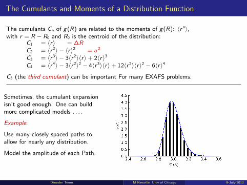
The Cumulants and Moments of a Distribution Function

The cumulants Cn of g(R) are related to the moments of g(R): 〈rn〉,with r = R − R0 and R0 is the centroid of the distribution:

C1 = 〈r〉 = ∆RC2 = 〈r 2〉 − 〈r〉2 = σ2

C3 = 〈r 3〉 − 3〈r 2〉〈r〉+ 2〈r〉3C4 = 〈r 4〉 − 3〈r 2〉2 − 4〈r 3〉〈r〉+ 12〈r 2〉〈r〉2 − 6〈r〉4

C3 (the third cumulant) can be important For many EXAFS problems.

Sometimes, the cumulant expansionisn’t good enough. One can buildmore complicated models . . . .

Example:

Use many closely spaced paths toallow for nearly any distribution.

Model the amplitude of each Path.


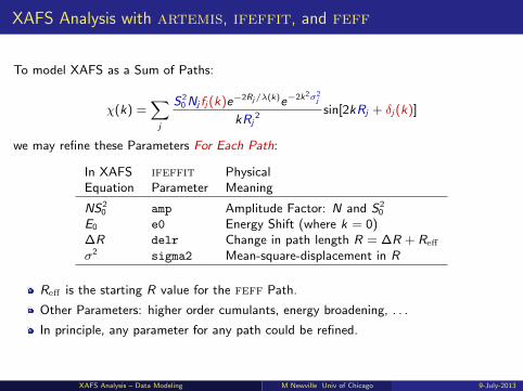
XAFS Analysis with artemis, ifeffit, and feff

To model XAFS as a Sum of Paths:

χ(k) =∑j


j


we may refine these Parameters For Each Path:

In XAFS ifeffit PhysicalEquation Parameter Meaning

NS20 amp Amplitude Factor: N and S2

0

E0 e0 Energy Shift (where k = 0)∆R delr Change in path length R = ∆R + Reff

σ2 sigma2 Mean-square-displacement in R

Reff is the starting R value for the feff Path.

Other Parameters: higher order cumulants, energy broadening, . . .

In principle, any parameter for any path could be refined.

XAFS Analysis – Data Modeling M Newville Univ of Chicago 9-July-2013

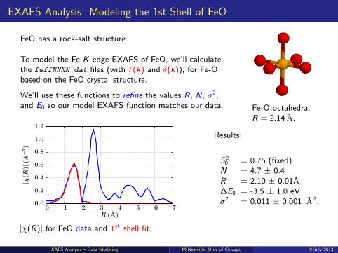
EXAFS Analysis: Modeling the 1st Shell of FeO

FeO has a rock-salt structure.

To model the Fe K edge EXAFS of FeO, we’ll calculatethe feffNNNN.dat files (with f (k) and δ(k)), for Fe-Obased on the FeO crystal structure.

We’ll use these functions to refine the values R, N, σ2,and E0 so our model EXAFS function matches our data. Fe-O octahedra,

R = 2.14 A.

R (A)

|χ(R

)|(A

−3)

76543210

1.2

1.0

0.8

0.6

0.4

0.2

0.0

|χ(R)| for FeO data and 1st shell fit.

Results:

S20 = 0.75 (fixed)

N = 4.7 ± 0.4R = 2.10 ± 0.01A∆E0 = -3.5 ± 1.0 eVσ2 = 0.011 ± 0.001 A2.


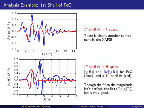
Analysis Example: 1st Shell of FeO

k (A−1)

k2χ(k

)(A

−2)

14121086420

1.5

1.0

0.5

0.0

-0.5

-1.0

-1.5

1st shell fit in k space.

There is clearly another compo-nent in the XAFS!

R (A)

|χ(R

)|(A

−3)

76543210

1.21.00.80.60.40.20.0

-0.2-0.4-0.6-0.8

1st shell fit in R space.

|χ(R)| and Re[χ(R)] for FeO(blue), and a 1st shell fit (red).

Though the fit to the magnitudeisn’t perfect, the fit to Re[χ(R)]looks very good.


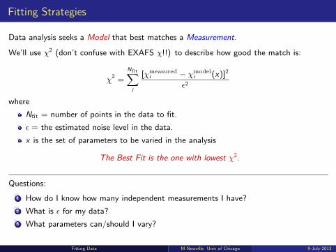
Fitting Strategies

Data analysis seeks a Model that best matches a Measurement.

We’ll use χ2 (don’t confuse with EXAFS χ!!) to describe how good the match is:

χ2 =

Nfit∑i

[χmeasuredi − χmodel

i (x)]2

ε2

where

Nfit = number of points in the data to fit.

ε = the estimated noise level in the data.

x is the set of parameters to be varied in the analysis

The Best Fit is the one with lowest χ2.

Questions:

1 How do I know how many independent measurements I have?

2 What is ε for my data?

3 What parameters can/should I vary?

Fitting Data M Newville Univ of Chicago 9-July-2013

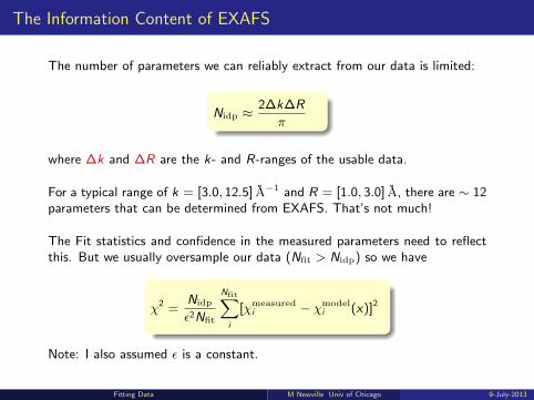
The Information Content of EXAFS

The number of parameters we can reliably extract from our data is limited:

Nidp ≈2∆k∆R

π

where ∆k and ∆R are the k- and R-ranges of the usable data.

For a typical range of k = [3.0, 12.5] A−1 and R = [1.0, 3.0] A, there are ∼ 12parameters that can be determined from EXAFS. That’s not much!

The Fit statistics and confidence in the measured parameters need to reflectthis. But we usually oversample our data (Nfit > Nidp) so we have

χ2 =Nidp

ε2Nfit

Nfit∑i

[χmeasuredi − χmodel

i (x)]2

Note: I also assumed ε is a constant.


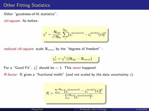
Other Fitting Statistics

Other “goodness-of-fit statistics”:

chi-square: As before:

χ2 =Nidp

ε2Nfit

Nfit∑i

[χmeasuredi −χmodel

i (x)]2

reduced chi-square: scale Nvarys by the “degrees of freedom” :

χ2ν = χ2/(Nidp − Nvarys)

For a “Good Fit”, χ2ν should be ∼ 1. This never happens!

R-factor: R gives a “fractional misfit” (and not scaled by the data uncertainty ε):

R =

∑Nfiti [χmeasured

i − χmodeli (x)]2∑Nfit

i [χmeasuredi ]2


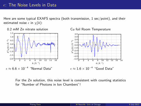
ε: The Noise Levels in Data

Here are some typical EXAFS spectra (both transmission, 1 sec/point), and theirestimated noise ε in χ(k):

0.2 mM Zn nitrate solution Cu foil Room Temperature

k (A−1)

k2χ(k

)(A

−2)

1614121086420

1.5

1.0

0.5

0.0

-0.5

-1.0

-1.5

-2.0

k (A−1)

k2χ(k

)(A

−2)

181614121086420

4.0

3.0

2.0

1.0

0.0

-1.0

-2.0

-3.0

-4.0

-5.0

ε ≈ 6.6× 10−4 “Normal Data” ε ≈ 1.6× 10−4 “Good Data”

For the Zn solution, this noise level is consistent with counting statisticsfor “Number of Photons in Ion Chambers”!


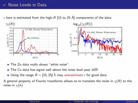
ε: Noise Levels in Data

ε here is estimated from the high-R [15 to 25 A] components of the data:

|χ(R)| log10(|χ(R)|)

Zn solution

Cu foil, Room Temerature

R(A)

|χ(R

)|(A

−3)

1086420

4.5

4.0

3.5

3.0

2.5

2.0

1.5

1.0

0.5

0.0

Zn solution

Cu foil, Room Temerature

R(A)

|χ(R

)|(A

−3)

302520151050

1

0.1

0.01

0.001

The Zn data really shows “white noise”.

The Cu data has signal well above the noise level past 10A!

Using the range R = [15, 25] A may overestimate ε for good data.

A general property of Fourier transforms allows us to translate the noise in χ(R) to thenoise in χ(k).


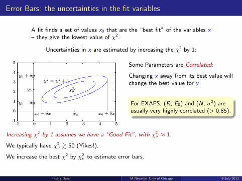
Error Bars: the uncertainties in the fit variables

A fit finds a set of values x0 that are the “best fit” of the variables x– they give the lowest value of χ2.

Uncertainties in x are estimated by increasing the χ2 by 1:

χ2 = χ20 + 1

χ20

y0 + δy

y0 − δy

x0 + δxx0 − δx

y0

x0

543210-1

5

4

3

2

1

0

-1

Some Parameters are Correlated:

Changing x away from its best value willchange the best value for y .

For EXAFS, (R, E0) and (N, σ2) areusually very highly correlated (> 0.85).

Increasing χ2 by 1 assumes we have a “Good Fit”, with χ2ν ≈ 1.

We typically have χ2ν & 50 (Yikes!).

We increase the best χ2 by χ2ν to estimate error bars.


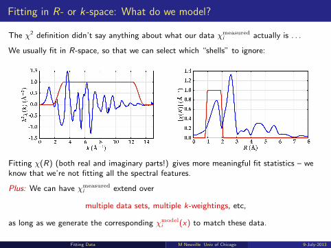
Fitting in R- or k-space: What do we model?

The χ2 definition didn’t say anything about what our data χmeasuredi actually is . . .

We usually fit in R-space, so that we can select which “shells” to ignore:

Fitting χ(R) (both real and imaginary parts!) gives more meaningful fit statistics – weknow that we’re not fitting all the spectral features.

Plus: We can have χmeasuredi extend over

multiple data sets, multiple k-weightings, etc,

as long as we generate the corresponding χmodeli (x) to match these data.


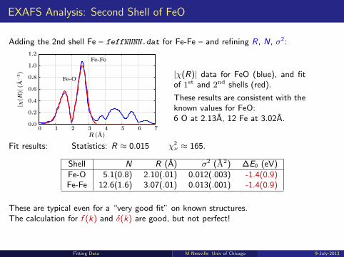
EXAFS Analysis: Second Shell of FeO

Adding the 2nd shell Fe – feffNNNN.dat for Fe-Fe – and refining R, N, σ2:

Fe-Fe

Fe-O

R (A)

|χ(R

)|(A

−3)

76543210

1.2

1.0

0.8

0.6

0.4

0.2

0.0

|χ(R)| data for FeO (blue), and fitof 1st and 2nd shells (red).

These results are consistent with theknown values for FeO:6 O at 2.13A, 12 Fe at 3.02A.

Fit results: Statistics: R ≈ 0.015 χ2ν ≈ 165.

Shell N R (A) σ2 (A2) ∆E0 (eV)Fe-O 5.1(0.8) 2.10(.01) 0.012(.003) -1.4(0.9)Fe-Fe 12.6(1.6) 3.07(.01) 0.013(.001) -1.4(0.9)

These are typical even for a “very good fit” on known structures.The calculation for f (k) and δ(k) are good, but not perfect!


EXAFS Analysis: Second Shell of FeO

Other views of the data and fit:

Fe-Fe

Fe-O

k (A−1)

k2χ(k

)(A

−2)

14121086420

1.5

1.0

0.5

0.0

-0.5

-1.0

-1.5

-2.0

-2.5

-3.0

The Fe-Fe EXAFS extends to higher-kthan the Fe-O EXAFS.

Even in this simple system, there issome overlap of shells in R-space.

The fit in Re[χ(R)] look especially good– this is how the fits are done.

Fe-Fe

Fe-O

R (A)

|χ(R

)|(A

−3)

76543210

1.2

1.0

0.8

0.6

0.4

0.2

0.0

Fe-Fe

Fe-O

R (A)

|χ(R

)|(A

−3)

76543210

1.21.00.80.60.40.20.0

-0.2-0.4-0.6-0.8-1.0


Path Parameters: what can we vary in a fit?

The EXAFS Equation has at least 4 adjustable parametes Per Path: E0, NS20 ,

R, and σ2. But Nidp is low:

Nidp = 8 for ∆R = 1 A and ∆k = 12.5 A−1

For simple crystalline structures with well-isolated, single-scattering path (likeFeO), it’s OK to fit N, R, σ2, and E0 for every path.

For more complicated problems, we need a way to limit the number of parametersvaried.

We might want to impose relationships between parameters to get more mean-ingful results. . .


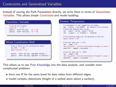
Constraints and Generalized Variables

Instead of varying the Path Parameters directly, we write them in terms of GeneralizedVariables. This allows simple Constraints and model building:

Parameter=Variable

# one e0 for 2 paths

guess e0 = 1.0

path(1, feff= feo.dat, e0 = e0)

path(2, feff= fefe.dat, e0 = e0)

Mixed Coordination Shell

# mix O and S in 1st coordination shell

set S02 = 0.80

guess xSulfur = 0.5

path(1, feff= feo.dat, amp=S02* xSulfur )

path(2, feff= fes.dat, amp=S02* (1-xSulfur) )

Einstein Temperature

# 1 parameter to set sigma2 for all paths

set factor = 24.254337 #= (hbar*c)^2/(2 k_boltz)

# mass and reduced mass in amu

set mass1 = 63.54, mass2 = 63.54

set r_mass = 1/ (1/mass1 + 1/mass2)

# the Einstein Temp will be adjusted in the fit!

guess thetaE = 200

# use for data set 1, T=77

set temp1 = 77

def ss2_path1 = factor*coth(thetaE/(2*temp1))/r_mass )

path(101, sigma2 = ss2_path1 )

# use for data set 2, T=300

set temp2 = 300

def ss2_path2 = factor*coth(thetaE/(2*temp2))/r_mass )

path(201, sigma2 = ss2_path2 )

This allows us to use Prior Knowledge into the data analysis, and consider morecomplicated problems:

force one R for the same bond for data taken from different edges.

model complex distortions (height of a sorbed atom above a surface).


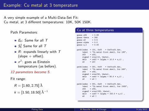
Example: Cu metal at 3 temperature

A very simple example of a Multi-Data-Set Fit:Cu metal, at 3 different temperatures: 10K, 50K 150K.

Path Parameters:

E0: Same for all T

S20 Same for all T

R: expands linearly with T(slope + offset).

σ2: goes as Einsteintemperature (as before).

12 parameters become 5.

Fit range:

R = [1.60, 2.75] A

k = [1.50, 18.50] A−1

Cu at three temperatures

guess s02 = 0.93

guess theta = 240

guess e0 = 3.5

guess alpha = 0.0

guess a_t = 0.00

path(index = 101, feff = feffcu01.dat,

label = "Cu metal first shell, for 10K",

s02 = s02,

sigma2 = eins(10, theta),

delr = reff * (alpha + 10.0 * a_t) ,

e0 = e0)



s02 = s02,



e0 = e0 )



s02 = s02,



e0 = e0 )


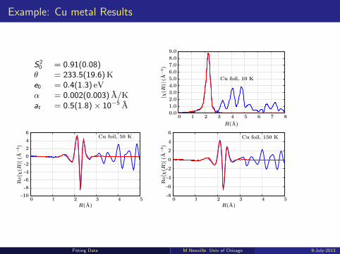
Example: Cu metal Results

S20 = 0.91(0.08)θ = 233.5(19.6)Ke0 = 0.4(1.3) eVα = 0.002(0.003) A/Kat = 0.5(1.8)× 10−5 A

Cu foil, 10 K

R(A)

|χ(R

)|(A

−3)

876543210

9.0

8.0

7.0

6.0

5.0

4.0

3.0

2.0

1.0

0.0

Cu foil, 50 K

R(A)

Re[χ

(R)]

(A−

3)

543210

6

4

2

0

-2

-4

-6

-8

-10

Cu foil, 150 K

R(A)

Re[χ

(R)]

(A−

3)

543210

6

4

2

0

-2

-4

-6

-8


Multiple Scattering Example: Cp-MnCO3

Cp-MnCO3 = tricarbonyl(η5-cyclopentadienyl)manganese(I)This molecule has linear Mn-C-O bonds, and two distinct Mn-C distances.

To model the EXAFS, we need thesepaths:

ring5 Mn-C at ∼ 2.13 A

carbonyl3 Mn-C at ∼ 1.78 A3 Mn-O at ∼ 2.93 A6 Mn-C-O paths at ∼ 2.93 A3 Mn-C-O-C paths at ∼ 2.93 A

The Multiple Scattering Paths will overlap the longer Mn-C(ring) distance!!Using only the single-scattering paths will gives:

large coordination numbers: 6 Mn-C(ring) at 2.10 A, 10Mn-C(carbonyl) at 1.80 A , and 10 Mn-O (carbonyl) at 2.99 A.

E0 of -13eV (pretty big! A hint!).


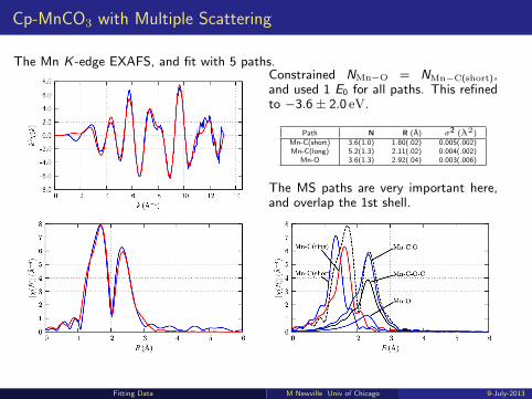
Cp-MnCO3 with Multiple Scattering

The Mn K -edge EXAFS, and fit with 5 paths.Constrained NMn−O = NMn−C(short),and used 1 E0 for all paths. This refinedto −3.6± 2.0 eV.

Path N R (A) σ2 (A2)

Mn-C(short) 3.6(1.0) 1.80(.02) 0.005(.002)Mn-C(long) 5.2(1.3) 2.11(.02) 0.004(.002)

Mn-O 3.6(1.3) 2.92(.04) 0.003(.006)

The MS paths are very important here,and overlap the 1st shell.


Conclusions

EXAFS Analysis is challenging:

1 Lots of Paths.

2 f (k), δ(k) are not trivial.

3 There’s not much information in a real measurement: Nidp ≈ 2∆k∆Rπ

We need to:

1 reduce the number of Paths to consider (Fourier analysis).

2 re-use feff calculations for f (k) and δ(k).

3 recycle parameters to cut down the number of independent variablesin the fit, while keeping a meaningful analysis.

Build physical models with Constraints

Study the error bars and correlations.

Find the simplest interpretation of your data.


EXAFS Analysis - X-ray Absorption

Documents

Transcript of EXAFS Analysis - X-ray Absorption