Journal of Empirical Finance 17 (2010) 180–194

Contents lists available at ScienceDirect

Journal of Empirical Finance

j ourna l homepage: www.e lsev ie r.com/ locate / jempf in

Exact inference and optimal invariant estimation for the stability parameterof symmetric α-stable distributions☆

Jean-Marie Dufour a,⁎, Jeong-Ryeol Kurz-Kim b

a Department of Economics, McGill University, Leacock Building, Room 519, 855 Sherbrooke Street West, Montréal, Québec, Canada H3A 2T7b Deutsche Bundesbank, Wilhelm-Epstein-Strasse 14, 60431 Frankfurt am Main, Germany

a r t i c l e i n f o

☆ The views expressed in this paper are those of th⁎ Corresponding author.

E-mail addresses: jean-marie.dufour@mcgill.ca (J.-1 Kurz-Kim and Loretan (2007), for example, revisit

Asset Pricing Model driven by Fama and French (1992

0927-5398/$ – see front matter © 2009 Elsevier B.V.doi:10.1016/j.jempfin.2009.09.001

a b s t r a c t

Available online 29 September 2009

Hill estimation (Hill, 1975), the most widespread method for estimating tail thickness ofheavy-tailed financial data, suffers from two drawbacks. One is that the optimal number of tailobservations to use in the estimation is a function of the unknown tail index being estimated,which diminishes the empirical relevance of the Hill estimation. The other is that thehypothesis test of the underlying data lying in the domain of attraction of an α-stable law(α<2) or of a normal law (α≥2) for finite samples, is performed on the basis of the asymptoticdistribution, which can be different from those for finite samples. In this paper, using theMonteCarlo technique, we propose an exact test method for the stability parameter of α-stabledistributions which is based on the Hill estimator, yet is able to provide exact confidenceintervals for finite samples. Our exact test method automatically includes an estimationprocedure which does not need the assumption of a known number of observations on thedistributional tail. Empirical applications demonstrate the advantages of our new method incomparison with the Hill estimation.

© 2009 Elsevier B.V. All rights reserved.

JEL Classification:C1C15C22G0E0

Keywords:α-Stable distributionHill estimatorMonte Carlo testHodges–Lehmann estimatorExact confidence intervalFinite sample

1. Introduction

Since the influentialwork byMandelbrot (1963),α-stable distributions haveoftenbeen considered amore realistic distribution forhigh-frequency variables, such as financial data, than the normal distribution, because asset returns, for example, are typically heavy-tailed and excessively peaked around zero—a phenomena that can be captured by α-stable distributions with α<2.

Statistical inferences for estimations and hypothesis tests under the α-stable distributional assumption depend crucially on α(DuMouchel, 1971).1 Therefore, one of the most important tasks in using the α-stable distribution is to precisely estimate α and tofind exact confidence intervals for finite samples for estimated α. To discriminate α<2 (domain of attraction of an α-stable law,Paretian case) from α≥2 (domain of attraction of normal law), or rather α=2 (Gaussian case), would be one example of howimportant it is to know what the exact confidence interval for the estimated α is.

Because of its simplicity and well-developed asymptotic properties, the Hill estimator (Hill, 1975) is the most popular methodfor estimating the tail thickness of empirical data, the stability parameter in the context of α-stable distributions. It is a simplenonparametric estimator based on order statistics. A severe drawback of the Hill estimator, however, is that it depends heavily onthe number of tail observations used. In practice, the optimal number of observations on the distributional tail is generallyunknown and depends on an unknown α. Another drawback is that its confidence interval for finite samples can be given only

e authors and not necessarily those of the Deutsche Bundesbank.

M. Dufour), jeong-ryeol.kurz-kim@bundesbank.de (J.-R. Kurz-Kim).the CRSP data used in Fama and French (1992) and show that the empirical conclusion about the Capita) is not robust depending on the distributional assumption for the underlying data.

All rights reserved.

l

181J.-M. Dufour, J.-R. Kurz-Kim / Journal of Empirical Finance 17 (2010) 180–194

based on the asymptotic distribution, which generally differ from the finite sample distributions. The Pickands (Pickands, 1975)and Dekkers, Einmahl and de Haan estimators (Dekkers et al., 1989) are variations on the Hill estimator. Some modifications arealso considered bymany authors. Huisman et al. (2001), for example, propose aweightedHill estimator that takes into account thetrade-off between bias and variance of the Hill estimator. However, for all the modified estimators of the Hill estimator, say, Hill-type estimators, the assumption of a known number of observations on the distributional tail is necessary, and confidenceintervals for finite samples can be given only based on the asymptotic distribution.2

In this paper, we propose an estimation procedure based on the Hill estimator which automatically results from an exact testmethod viaMonte Carlo (MC) technique (Dufour, 2006)3 (henceforth referred to as theMC test or theMC estimation). This is becausean exact confidence interval for finite samples can be constructed in the estimation procedures, or rather, an estimate in the testprocedure. The novelty of the paper is, however, that we do not use the Hill estimator as a direct estimate of α, but rather as a pivotalstatistic onwhich to base our estimate ofα. In so doing, ourMCmethod improves on the (direct) Hill estimation in twoways. First, theoptimal number of observations on the distributional tail does not need (to be assumed) to be known for our estimator, i.e. it can varyoptimally with the unknown α. Second, our estimator provides exact confidence intervals for finite samples.

The rest of the paper is structured as follows. Section 2 gives a brief summary of α-stable distributions and the Hill estimator.Consequently, the problem of choice of optimal k is discussed. Two practical problems for applying the Hill estimator, the two-tailedHill estimator and the relocation of empirical data, are also discussed. In Section 3, after a brief summary of theMC technique, theMCestimation and test procedure are explained. In Section 4, we perform simulations to study the size of the usual asymptotic test andpowerof theMC test forfinite samples. An empirical application is given in Section5 todemonstrate the advantage of ournewmethodover the Hill estimation. Section 6 summarizes the paper.

2. Framework

2.1. A brief summary of α-stable distributions

A random variable (r.v.) X is said to be stable if, for any positive numbers A and B, there is a positive number C and a real numberD such that AX1 + BX2 =d CX + D, where X1 and X2 are independent r.v.s with Xi =

d X; i = 1;2; and “=d ” denotes equality indistribution. Moreover, C=(Aα+Bα)1/α for some α∈ (0, 2], where the exponent α is called a stability parameter. A stable r.v., X, witha stability parameter α is called α-stable. The α-stable distributions are described by four parameters denoted by S(α, β, μ, σ).Although theα-stable laws are absolutely continuous, their densities canbe expressed only by a complicated special functionexcept inthree special cases.4 Therefore, the logarithmof the characteristic function of theα-stable distribution is the bestway of characterizingall members of this family and is given as

2 Foruses a bto the d

3 Anthe bas

4 Thesymme

lnZ ∞

�∞eistdPðX < xÞ =

�σα jt jα 1� iβ sign ðtÞ tanπα2

h i+ iμt; for α≠ 1;

�σ jt j 1 + iβπ2sign ðtÞ ln jt j

h i+ iμt; for α = 1:

8><>:

The shape of theα-stable distribution is determined by the stability parameter α. For α=2 the α-stable distribution reduces tothe normal distribution, which is the only member of the α-stable family with finite variance. If α<2, moments of order α orhigher do not exist and the tails of the distribution become thicker, i.e. the magnitude and frequency of outliers (from theviewpoint of the Gaussian) increase as α decreases. Skewness is governed by β∈ [−1,1]. If β=0, the distribution is symmetric.The location and scale of the α-stable distributions are denoted by μ and σ. The standardized version of the α-stable distribution isgiven by S((x−μ)/σ; α, β, 0,1). The present paper considers only the symmetric case, i.e. we assume β=0 throughout.

A strong argument in favor of the α-stable distribution as a distributional assumption for heavy-tailed empirical data is that onlythe α-stable distribution can serve as the limiting distribution of sums of independent identically distributed (i.i.d.) r.v.s proved byZolotarev (1986). Formore details on theα-stable distributions, see Zolotarev (1986) and Samorodnitsky and Taqqu (1994); and for adiscussionof the role of theα-stable distributions infinancialmarkets andmacroeconomicmodelling, seeMcCulloch (1996), Kimet al.(1997) and Rachev et al. (1999).

2.2. Hill estimator, choice of the number of tail observations and relocation

2.2.1. Hill estimatorThe most popular method of estimating for α is the Hill estimator (Hill, 1975), which is a simple nonparametric estimator

based on order statistics. Because of its simplicity and popularity, we use the Hill estimator for constructing our test statistic

a rough check, the quantile estimation of McCulloch (1986) may be used. The maximum likelihood (ML) estimation is also available: DuMouchel (1971)inned approximate ML based on the cumulative distribution function. McCulloch (1998) considers symmetric stable ML using a numerical approximationensity. But these are more complicated and computationally intensive than the Hill estimator.estimation procedure which is based on the MC method is termed a Hodges–Lehmann estimation in the literature. See Hodges and Lehmann (1963) foric idea.three special cases, in which the densities are expressible via elementary functions, are i) the Gaussian distribution S(2,0,μ,σ)≡N(μ,2σ2), ii) the

tric Cauchy distribution S(1,0,μ,σ), and iii) the Lévy distribution S(0.5,±1,μ,σ); see Zolotarev (1986).

182 J.-M. Dufour, J.-R. Kurz-Kim / Journal of Empirical Finance 17 (2010) 180–194

although any consistent estimator can be used to formulate our test statistic. Given a sample of n observations, X1, X2,…, Xn, the(upper-tail) Hill estimator5 is given as

5 Becin the e

6 The7 Bec

estimat

αH = k�1∑k

j=1ln Xn+1�j:n � ln Xn�k:n

� �" #�1

; ð1Þ

k is the number of tail observations used and Xj:n denotes the j-order statistic of the sample size n. If the tail of the

wheredistribution is asymptotically Pareto, which for 0<α<2 is in the domain of attraction of the α-stable Paretian law, αH is used asestimate for the stability parameter. The asymptotic properties of the Hill estimator have been studied by many authors and arewell developed: Goldie and Smith (1987) prove asymptotic normality of the Hill estimator, i.e.

ffiffiffik

pα�1

H � α�1� �

∼N 0;α�2� �

: ð2Þ

Mason (1982) and Hsing (1991) consider weak consistency of the Hill estimator for independent and dependent cases. Thestrong consistency is proved by Deheuvels et al. (1988). Although the asymptotic properties of the Hill estimator are well known,little can be said about its finite sample performance.

2.2.2. Choice of optimal kBefore we estimate the stability parameter using the Hill estimator, one practical problem needs to be solved: how to choose

optimally the number of observations on the distributional tail, k, which are contained in the Hill estimator. Note that the choice of kinvolves a trade-off, because it must be small enough for the observation Xn−k:n to characterize the asymptotic power tail of thedistribution. If it is too small, however, the estimator will lack precision. For more analytic details on this issue see Segers (2002). Inpractice, k is determined more or less by intuition or rather arbitrarily in the Hill estimation. This is a severe drawback for the Hillestimation in terms of empirical relevance and, as far aswe know, there is no statistical consensus to determine k. Some authors havelooked into the problem. DuMouchel (1983) proposes setting the combined k from both tails equally to 10% of samples as kindependent of n andα, which, aswill be shown, can be optimal onlywhenα is very small and n is very large. Beirlant et al. (1996), forinstance, consider a couple of the quantile-plot methods that can be implemented and used in empirical work. Therefore, from thepractical point of view, our MC estimation, for which k does not need to be known, is of empirical importance.

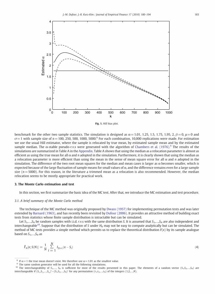
In order to demonstrate the problem of the dependence of k on the unknown α, we show the so-called Hill bias plot. Fig. 1 showsHill estimates for which the data come from anα-stable distributionwith α=1.75 and a sample size of 1000.6 The values of k plottedare in steps of 10 from 10 (the ten largest observations in absolute value) to 990. For each value of k, 100,000 replications are made.

The solid line shows the mean of the 100,000 estimates for each k and the dashed lines above and below of the decreasing solidline show 95% Monte Carlo confidence intervals. The straight solid line means the true value of α is 1.75.

Fig. 1 shows clearly that the Hill estimate is extremely sensitive to the choice of k. Depending on k, almost every value of α ispossible for empirical data. But the true α=1.75 can be mostly detected for a certain k, namely k=430.7 Furthermore, Fig. 1 alsoshows that estimates of the stability parameter larger than 2 in empirical applications are not necessarily evidence against infinite-variance stable distributions with α<2, as is pointed out in McCulloch (1997). A bad choice of k is often misleadingwith respect tothe true tail thickness.

2.3. Two-tailed Hill estimator and median relocation

In this subsection, we discuss some aspects raised in practical applications of the Hill estimator in Eq. (1). The Hill estimator in Eq. (1)uses the largest k observations for estimating the stability parameter. For the symmetric case, especially for small samples, the two-tailedHill estimator based on the order statistics of the absolute values can be also used in order to achieve high estimation efficiency, as:

α2H = k�1∑k

j=1ln jX jn+1�j:n � ln jX jn�k:n

� �" #�1

; ð3Þ

, for the same n, k here is two times the k in the one-tailed case in Eq. (1). For practical applications, the data must somehow

wherebe relocated, because the estimator in Eq. (3) is scale-invariant, but not location-invariant. Despite the existence of the firstmoment for 1<α<2, the mean often cannot serve optimally as a relocation parameter because of its fluctuation, especially whenα is small. Therefore, the median is an alternative choice as a relocation parameter.

Regarding relocation, we perform a simulation study. The simulation shows the efficiency of the Hill estimator among threerelocations; true mean, sample mean and sample median. The case for true mean is not of empirical relevance, but it serves as a

ause we consider only the symmetric case, we will use the two tails later in the paper in order to obtain more tail observations and, hence, more efficiencystimation.results for other α values and sample sizes are the same as that for 1000 with respect to the main conclusion.ause our MC procedure, as will be shown, uses such k determined by simulation under the null hypothesis (i.e. by known α), in this sense our MCe can be regarded as optimal.

8 If α=1 the true mean doesn't exist. We therefore use α=1.01 as the smallest value.9 The same random generator will be used for all the following simulations.

10 The interchangeability of S1,…, SN is sufficient for most of the results presented in this paper. The elements of a random vector (S1,S2,…,SN) areinterchangeable if (Sr1,Sr2,…,SrN)′~(S1,S2,…,SN)′ for any permutation (r1,r2,…,rN) of the integers (1,2,…,N).

Fig. 1. Hill bias plot.

183J.-M. Dufour, J.-R. Kurz-Kim / Journal of Empirical Finance 17 (2010) 180–194

benchmark for the other two sample statistics. The simulation is designed as α=1.01, 1.25, 1.5, 1.75, 1.95, 2, β=0, μ=0 andσ=1 with sample size of n=100, 250, 500, 1000, 5000.8 For each combination, 10,000 replications were made. For estimationwe use the usual Hill estimator, where the sample is relocated by true mean, by estimated sample mean and by the estimatedsample median. The α-stable pseudo-r.v.s were generated with the algorithm of Chambers et al. (1976).9 The results of thesimulations are summarized in Table A in the Appendix. Table A shows that using themedian as a relocation parameter is almost asefficient as using the true mean for all α and n adopted in the simulation. Furthermore, it is clearly shown that using the median asa relocation parameter is more efficient than using the mean in the sense of mean square error for all α and n adopted in thesimulation. The difference of the two root mean squares for the median and mean cases is larger as α becomes smaller, which isexpected because of the large fluctuation of samplemeans for small values of α, and the difference remains even for a large samplesize (n=5000). For this reason, in the literature a trimmed mean as a relocation is also recommended. However, the medianrelocation seems to be mostly appropriate for practical work.

3. The Monte Carlo estimation and test

In this section, we first summarize the basic idea of the MC test. After that, we introduce the MC estimation and test procedure.

3.1. A brief summary of the Monte Carlo method

The technique of the MC method was originally proposed by Dwass (1957) for implementing permutation tests and was laterextended by Barnard (1963), and has recently been revisited by Dufour (2006). It provides an attractive method of building exacttests from statistics whose finite sample distribution is intractable but can be simulated.

Let S1,…,SN be random samples with i.i.d. r.v.s with the same distribution S. It is assumed that S1,…,SN are also independent andinterchangeable10. Suppose that the distribution of S under H0 may not be easy to compute analytically but can be simulated. Themethod of MC tests provides a simple method which permits us to replace the theoretical distribution F(x) by its sample analoguebased on S1,…,SN as

FN ½x; SðNÞ� =1N

N∑

i = 1I½0;∞Þðx� SiÞ ð4Þ

be thevariab

then

and

where

whichintege

in whregionregiondetails

11 The12 For

See

184 J.-M. Dufour, J.-R. Kurz-Kim / Journal of Empirical Finance 17 (2010) 180–194

S(N)=(S1,…,SN), and IA(x) is the usual indicator function associated with the set A, i.e. IA(x)=1, when x∈A and 0

whereotherwise. Furthermore, let

GN ½x; SðNÞ� =1N

N∑

i = 1I½0;∞ÞðSi � xÞ ð5Þ

corresponding sample function of the tail area. The sample distribution function is related to the ranks R1,…,RN of theles S1,…,SN (when put in ascending order) by the expression:

Rj = N FN ½Sj; SðNÞ� = ∑N

i=1s Sj � Si� �

; j = 1;…;N: ð6Þ

The main idea of the MC method is that one can obtain critical values and/or compute p-values by replacing the “theoretical”null distribution F(x) through its simulation-based “estimate” F N(x) in a way that will preserve the level of the test in finitesamples, irrespective of the number N of replications used as follows. Let S0 be an empirical sample of interest, (S1,…,SN)′, a simulated(N×1)-, and consequently (S0,S1,…,SN)′, a ((N+1)×1)-randomvector of interchangeable real r.v.s.11Moreover, let FN(x)≡ FN[x; S(N)]and ĜN(x) =ĜN[x; S(N)] be defined as in Eqs. (4)–(5) and FN

−1(x) be the quantile function12 and set

pNðxÞ = N GNðxÞ + 1N + 1

: ð7Þ

P GNðS0Þ≤α1

h i= P FNðS0Þ≥1�α1

h i= I½α1N� + 1

N + 1; for 0≤α1≤1; ð8Þ

P S0≥ F�1N ð1� α1Þ

h i= I½α1N� + 1

N + 1; for 0 < α1 < 1; ð9Þ

P½ pNðS0Þ≤α� = I½αðN + 1Þ�N + 1

; for 0 ≤ α ≤1; ð10Þ

I[z]is the largest integer less than or equal to z. For practical purposes, α1 and N will be chosen as

α =I½α1N� + 1

N + 1; ð11Þ

is the desired significance level. Provided N is reasonably large, α1 will be very close to α; in particular, if α(N+1) is anr, we can take

α1 = α� ð1� αÞN

;

ich case we see easily that the critical region GN(S0)≤α1 is equivalent to GN(S0)<α. For 0<α<1, the randomized criticalS0 ≥ F N

−1(1−α1) has the same level (α) as the non-randomized critical region S0≥F−1(1−α), or equivalently the criticals pN(S0)≤α and G N(S0)≤α1 have the same level as the critical region G(S0)≡1−F(S0)≤α. See Dufour (2006) for moreon proofs and discussions about the MC test.

zero probability of ties is assumed, but the results are still valid for a positive probability of ties.any probability distribution function F(x), the quantile function F−1(q) is defined as follows:

F�1ðqÞ =inf x : FðxÞ≥q; if 0 < q < 1;

inf x : FðxÞN 0; if q = 0;

sup x : FðxÞ < 1; if q = 1:

8>><>>:

Reiss (1989, p. 13).

185J.-M. Dufour, J.-R. Kurz-Kim / Journal of Empirical Finance 17 (2010) 180–194

3.2. Finite sample estimation and test for the stability parameter

We now test our random sample, {X1,X2,…,Xn}, from a symmetric α-stable (SαS) distribution13 for

with Xconstrbetweas the

be an

then th

then th

13 In cstatistic14 Theby a lin

n

10025050010002000500010,00

15 Whbetweemean sq(see BoFurtherconditioof a dis

H0ðα0Þ : α = α0: ð12Þ

For our MC test the α0 is not a unique value, but, depending on a preliminary choice, several values. To make this clear, we usethe symbol H0(α0) instead of the usual H0. To perform this test, we need a test statistic which is free of nuisance parameters underthe null hypothesis. A possible statistic can be given as

STðα0Þ = α�α0; ð13Þ

αmay be any consistent estimator for α. The fact that αmay be any consistent estimator for αmeans that our MC method

wherecan provide any consistent estimator with an exact confidence interval for finite samples. Furthermore, we construct an estimatorfor each α0 assumed based on Eq. (3) and median relocation which can be used as α in Eq. (13):

αðα0Þ = kðα0Þ�1 ∑kðα0Þ

j=1ln jX jn + 1�j:n � ln jX jn�kðα0Þ:n

� �" #�1

; ð14Þ

i:=Xi−Xmed and k(α0)=k(n,α0) being the number of tail observations under each respective null hypothesis. Thisuction enables us to use any optimal k in some sense which is determined by a theoretical and/or a simulative relationshipen k andα. We adopt the k/n ratio tabulated by simulation in Rachev andMittnik (2000, p. 114). For a givenα, they choose the koptimal number of tail observations by which the mean of the estimates from the simulated samples with α is equal to α.14 Innse, we regard our MC estimation as optimal—at least for finite samples.15

this se

To estimate the stability parameter using our MC method, the test statistic in Eq. (13) should be nuisance-free. Because theestimator in Eq. (14) is location and scale-invariant, the test statistic in Eq. (13) is pivotal as proved in the following lemma.

Proposition 1. [Invariance] Let X1,X2,…,Xn be i.i.d. random variables which follow an S(α,β,μ,σ) distribution, and let

α = aðX1;X2;…;XnÞ ð15Þ

estimator of α. If the estimator α is scale-invariant, i.e.

α = aðcX1;…; cXnÞ = aðX1;X2;…;XnÞ; for all c N 0; ð16Þ

e estimator αhas a distribution which depends only on α, β and μ/σ. If, furthermore, α is location-scale-invariant, i.e.

α = aðcX1 + d;…; cXn + dÞ = aðX1;X2;…;XnÞ; for all c N 0 and d∈R; ð17Þ

e estimator α has a distribution which depends only on β.

ase of asymmetric data, our procedure can be also applied in the same way, as in the Hill estimation, for only one tail. Based on the Kolmogorov–Smirnov, Dufour et al. (2007) propose an estimation and test for the asymmetric parameter of α-stable distributions.k/n values for the two-tailed case are reproduced for selected n in the following table, where the intermediate values needed in the paper are calculatedear interpolation.

α

1.0 1.1 1.2 1.3 1.4 1.5 1.6 1.7 1.8 1.9

.23 .29 .35 .37 .39 .41 .42 .43 .44 .44

.168 .240 .324 .348 .380 .408 .420 .424 .432 .440

.140 .214 .308 .348 .378 .404 .418 .424 .432 .440

.121 .197 .295 .342 .378 .402 .417 .425 .431 .439

.0715 .1845 .2880 .3405 .3765 .3995 .4160 .4245 .4315 .4380

.0660 .1768 .2814 .3390 .3750 .3980 .4140 .4240 .4318 .43720 .0400 .1671 .2801 .3385 .3747 .3981 .4139 .4239 .4317 .4373

en implementing our method, there are other rules that may be used for determining k(n,α). One can easily employ any asymptotic relationshipsn k and α (see de Haan and Ferreira, 2006, Ch.3 for more details on the topic) which usually are determined, for instance, by minimizing the asymptoticuared error of the Hill estimate. The true tail behavior of α-stable laws, however, is visible only for extremely large data sets, possibly larger than 106

rak et al., 2005) which implies that the optimal k/n for finite samples can be vastly different from those calculated from such asymptotic relationships.more, whatever rule is used for determining k/n, the results from our method will be unchanged, because the rule that is chosen provides the samen in estimating for both the empirical data and the simulated data from every grid of α assumed under the null hypothesis. This footnote is the outcomecussion with an anonymous referee, whom we wish to thank very much.

186 J.-M. Dufour, J.-R. Kurz-Kim / Journal of Empirical Finance 17 (2010) 180–194

Proof 1. To obtain the first result, we observe that

fromcondit

Table 1Asympt

α

1

1.25

1.5

1.75

2

The usuTable).by DuM

Xi = σ∼Sðα;β; μ = σ;1Þ; i = 1;…;n: ð18Þ

Then, using the scale-invariance property (16) with c=1/σ, we can write

α = aðX1 = σ;…;Xn = σÞ; ð19Þ

which we see that the distribution of α depends only on α, β, and μ/σ. Similarly, under the location-scale invarianceion (17), we observe the following:

ðXi � μÞ = σ∼Sðα;β;0;1Þ; i = 1;…;n: ð20Þ

Hence, taking c=1/σ and d=−μ/σ

α = aðX1⁎;…;Xn

⁎Þ; ð21Þ

Xi⁎ = ðXi � μÞ= σ; i = 1;…;n:

where

Now, we introduce theMC estimation and test procedure for the stability parameter. Given a random sample {X1,X2,…,Xn} froma SαS distribution, the following seven steps are needed:

1. Determine the set of possible α under the null hypothesis. From the viewpoint of empirical relevance it is reasonable to assumethat α0∈ [1, 2].

2. Choose a rule k(α0)=k(n, α0) for selecting k as a function of n and α0.3. Using the empirical data, calculate the estimator in Eq. (14) and the test statistic in Eq. (13) for every point in a fine grid of α0

values in the set of possible values, in steps of 0.01, for example.

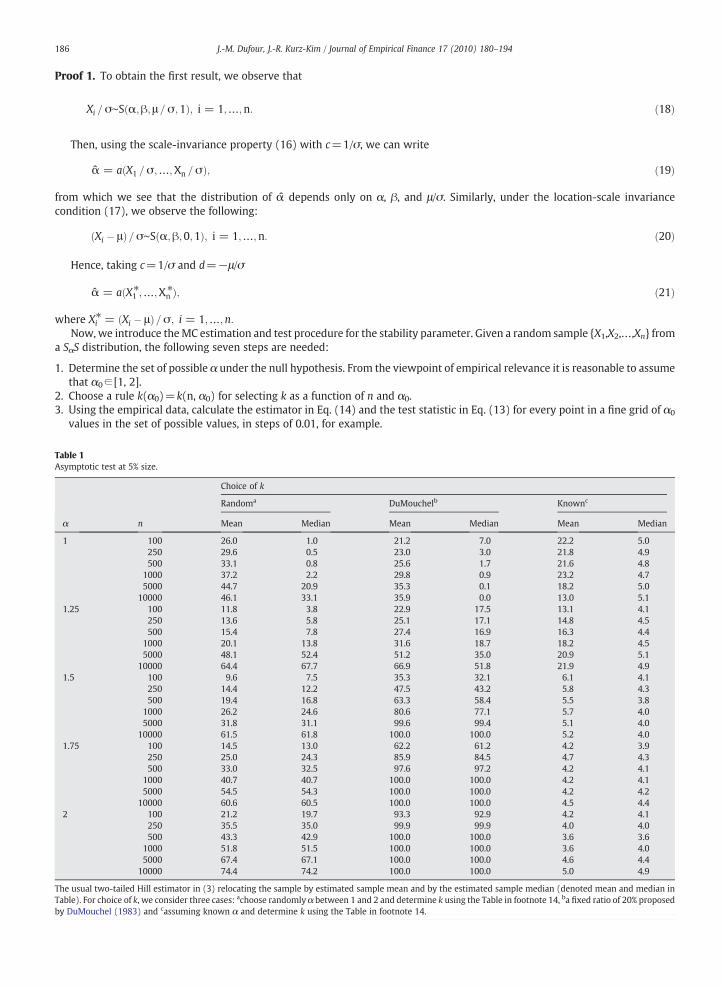
otic test at 5% size.

Choice of k

Randoma DuMouchelb Knownc

n Mean Median Mean Median Mean Median

100 26.0 1.0 21.2 7.0 22.2 5.0250 29.6 0.5 23.0 3.0 21.8 4.9500 33.1 0.8 25.6 1.7 21.6 4.8

1000 37.2 2.2 29.8 0.9 23.2 4.75000 44.7 20.9 35.3 0.1 18.2 5.0

10000 46.1 33.1 35.9 0.0 13.0 5.1100 11.8 3.8 22.9 17.5 13.1 4.1250 13.6 5.8 25.1 17.1 14.8 4.5500 15.4 7.8 27.4 16.9 16.3 4.4

1000 20.1 13.8 31.6 18.7 18.2 4.55000 48.1 52.4 51.2 35.0 20.9 5.1

10000 64.4 67.7 66.9 51.8 21.9 4.9100 9.6 7.5 35.3 32.1 6.1 4.1250 14.4 12.2 47.5 43.2 5.8 4.3500 19.4 16.8 63.3 58.4 5.5 3.8

1000 26.2 24.6 80.6 77.1 5.7 4.05000 31.8 31.1 99.6 99.4 5.1 4.0

10000 61.5 61.8 100.0 100.0 5.2 4.0100 14.5 13.0 62.2 61.2 4.2 3.9250 25.0 24.3 85.9 84.5 4.7 4.3500 33.0 32.5 97.6 97.2 4.2 4.1

1000 40.7 40.7 100.0 100.0 4.2 4.15000 54.5 54.3 100.0 100.0 4.2 4.2

10000 60.6 60.5 100.0 100.0 4.5 4.4100 21.2 19.7 93.3 92.9 4.2 4.1250 35.5 35.0 99.9 99.9 4.0 4.0500 43.3 42.9 100.0 100.0 3.6 3.6

1000 51.8 51.5 100.0 100.0 3.6 4.05000 67.4 67.1 100.0 100.0 4.6 4.4

10000 74.4 74.2 100.0 100.0 5.0 4.9

al two-tailed Hill estimator in (3) relocating the sample by estimated sample mean and by the estimated sample median (denoted mean and median inFor choice of k, we consider three cases: achoose randomly α between 1 and 2 and determine k using the Table in footnote 14, ba fixed ratio of 20% proposedouchel (1983) and cassuming known α and determine k using the Table in footnote 14.

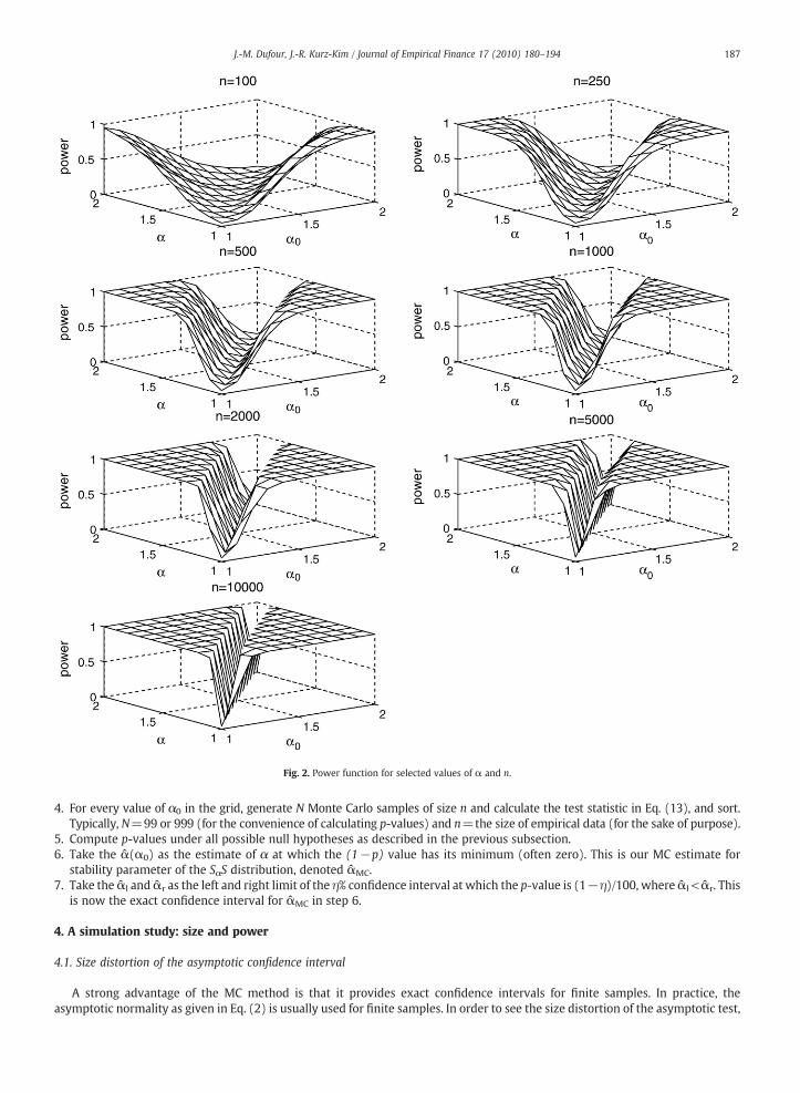
Fig. 2. Power function for selected values of α and n.

187J.-M. Dufour, J.-R. Kurz-Kim / Journal of Empirical Finance 17 (2010) 180–194

4. For every value of α0 in the grid, generate N Monte Carlo samples of size n and calculate the test statistic in Eq. (13), and sort.Typically, N=99 or 999 (for the convenience of calculating p-values) and n=the size of empirical data (for the sake of purpose).

5. Compute p-values under all possible null hypotheses as described in the previous subsection.6. Take the α(α0) as the estimate of α at which the (1−p) value has its minimum (often zero). This is our MC estimate for

stability parameter of the SαS distribution, denoted αMC.7. Take the αl and αr as the left and right limit of the η% confidence interval at which the p-value is (1−η)/100, where αl< αr. This

is now the exact confidence interval for αMC in step 6.

4. A simulation study: size and power

4.1. Size distortion of the asymptotic confidence interval

A strong advantage of the MC method is that it provides exact confidence intervals for finite samples. In practice, theasymptotic normality as given in Eq. (2) is usually used for finite samples. In order to see the size distortion of the asymptotic test,

16 If necessary, we choose the same k/n ratio α=1.9 for α=2.

Fig. 3. DAX returns in different frequencies.

188 J.-M. Dufour, J.-R. Kurz-Kim / Journal of Empirical Finance 17 (2010) 180–194

we perform a simulation study. The simulation is designed as α=1, 1.25, 1.5, 1.75,216, β=0, μ=0 and σ=1with a sample size ofn=100, 250, 500, 1000, 5000, 10,000. For each combination, 10,000 replications were made. We use the usual two-tailed Hillestimator in Eq. (3) relocating the sample by the estimated sample mean and by the estimated sample median. For our choice of k,we consider three cases: i) choose randomly α between 1 and 2 and determine k using the table in footnote 14, ii) a fixed ratio of20% proposed by DuMouchel (1983) and iii) assume a known α and determine k using the table in footnote 14. The result of thesimulation is summarized in Table 1, where the numbers in the table are percentage points of rejection. Although we only reportfor the 5% size, the other usual confidence levels show very similar results.

Some comments on Table 1 are in order. (1) the median relocation generally shows a better result for all α and n selected.Even in the known case, themedian relocation works better when α is small, because of the large fluctuation of the sample meanfor small α, as discussed in Subsection 2.3. (2) In a comparison of the three different choicemethods, the ratio of over-rejection istheworst for the fixed k, followed by the random choice, and is, as expected, best for the known case. The fixed percentage of 20%is, as can be seen in the table in Footnote 14, only appropriate for a small α, say 1.1, or even smaller α when n is very small.Because of that, the fixed percentage method is not appropriate in almost all cases considered, while the random choice can befrom time to time a proper one, just randomly. (3) Contrary to the general intuition, the general aggravation of the size distortionwhen n becomes large, at least for the random and the fixed method, can be explained because the large outliers for a small αwhich occur seldom have a better chance of being included in the sample when n is sufficiently large. (4) The size distortion ismore dramatic as α approaches 2, because the thinner the tail becomes, the more difficult to estimate it precisely, and it is wellknown that the Hill-type estimates have a bias as α approaches 2. This phenomenon has a severe consequence in empiricalstudies, because most empirical data have an α between 1.5 and 2 (see Kim et al., 1997) meaning that a careful choice of k, orrather, using a method without assuming known k, is of importance for empirical work. The results of the asymptotic test showthat it suffers generally from size distortion, even for the known case if α is small. Note that the sizes from ourMCmethod are, byconstruction, exact.

189J.-M. Dufour, J.-R. Kurz-Kim / Journal of Empirical Finance 17 (2010) 180–194

4.2. Power function of the Monte Carlo test

The theoretical size and power of the MC test is considered in Dufour (2006). Although the discrepancy of the correct size andthe superior power of the MC test over the conventional test go to zero as the sample size approaches infinity, the behavior of thepower function for the finite sample is usually of interest.

To check the power of ourMC test, we perform a simulation study by drawing from symmetric α-stable pseudo-r.v.s relocated bythe median. As pseudo-empirical data we use the same α-stable random sample generated earlier, and test H0: α=α0, where α0 isassumed to take on values from 1.0 to 2.0 in steps of 0.1. Sample sizes of n=100, 250, 500, 1000, 2000, 5000 and 10,000 are selected,and the number of replications is 10,000. To demonstrate the power function, we select a usual significance level of 95%. Fig. 2 showsthe power functions for the selected α, n and percentage points as described above.

As expected, the power converges to the corresponding ideal value for each given significance level as the sample size grows. Asample size of 2000 gives a rather satisfactory power. A large loss of power can be observed for extremely small sample sizes.

5. Empirical applications

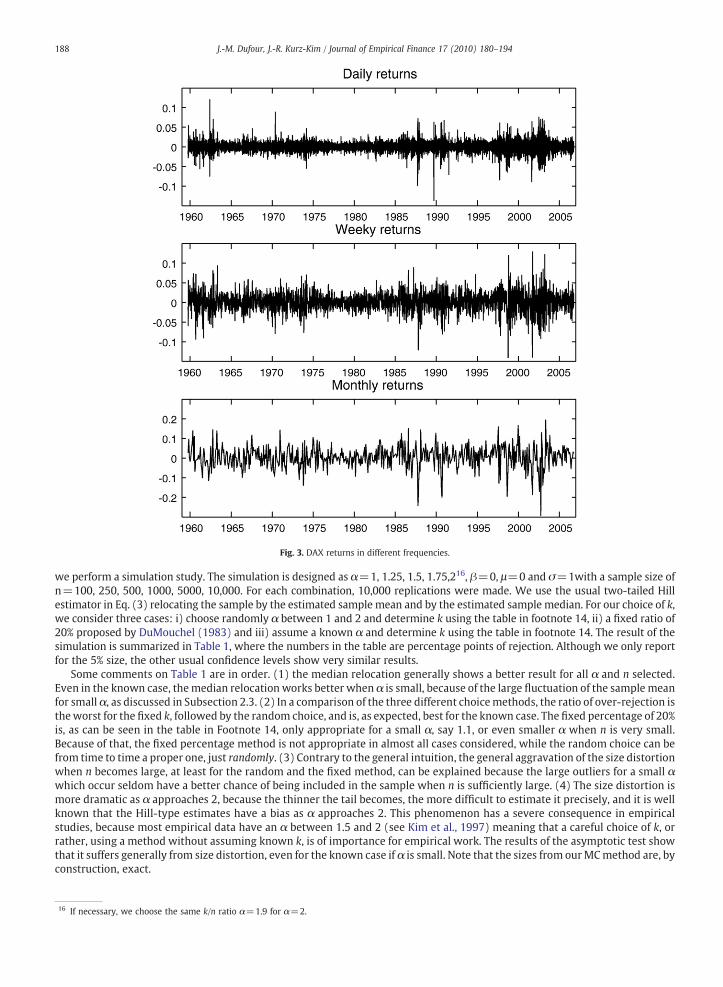
To illustrate the use of the Monte Carlo method in practice, we employ the German stock index from its beginning (1 October1959) to 30 September 2006 (47 years). For a deeper look, we consider them in three different frequencies, namely daily (11,796observations), weekly (2453 observations) and monthly (564 observations), where the observations for the weekly and monthlydata are those of the end of the period, i.e. the Friday values for the weekly data and the value at end of the each month for themonthly data. Fig. 3 shows the empirical data.

The volatility cluster looks, to a large extent, similar in three different frequencies. However, a careful look reveals that many ofthe single outliers in the daily returns are no longer seen in the weekly returns and vice versa. The same also applies between theweekly returns and the monthly ones. This is because the weekly and/or monthly data do not come from a moving average of thedaily data. (Even if the low frequency data come from a moving average of a higher frequency data, the two dynamics are notnecessarily the same or very similar.)

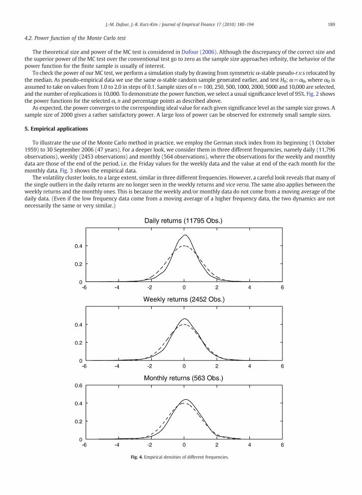
Fig. 4. Empirical densities of different frequencies.

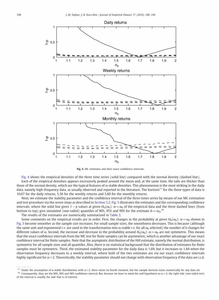
Fig. 5. MC estimates and their exact confidence intervals.

190 J.-M. Dufour, J.-R. Kurz-Kim / Journal of Empirical Finance 17 (2010) 180–194

Fig. 4 shows the empirical densities of the three time series (solid line) compared with the normal density (dashed line).Each of the empirical densities appears excessively peaked around the mean and, at the same time, the tails are thicker than

those of the normal density, which are the typical features of α-stable densities. This phenomenon is the most striking in the dailydata, namely high-frequency data, as usually observed and reported in the literature. The kurtosis17 for the three types of data is10.67 for the daily returns, 5.36 for the weekly returns and 5.60 for the monthly returns.

Next, we estimate the stability parameter and the confidence interval of the three times series by means of our MC estimationand test procedure via the seven steps as described in Section 3.2. Fig. 5 illustrates the estimates and the corresponding confidenceintervals, where the solid line gives 1−p values at given H0(α0): α=α0 of the empirical data and the three dashed lines (frombottom to top) give simulated (one-tailed) quantiles of 90%, 95% and 99% for the estimate α=α0.18

The results of the estimates are numerically summarized in Table 2.Some comments on the empirical results are in order. First, the changes in the probability at given H0(α0): α=α0 shown in

Fig. 5 become smoother as the sample size increases. For small sample sizes, the smoothness decreases. This is because (althoughthe same unit and exponential r.v. are used in the transformation into α-stable r.v. for all α0 selected) the number of k changes fordifferent values of α. Second, the increase and decrease in the probability around H0(α0): α=α0 are not symmetric. This meansthat the exact confidence intervals from theMC test for finite samples can be asymmetric, which is another advantage of our exactconfidence interval for finite samples. Note that the asymptotic distribution of the Hill estimate, namely the normal distribution, issymmetric for all sample sizes and all quantiles. Also, there is no statistical background that the distribution of estimates for finitesamples must be symmetric. Third, the estimated stability parameter for the daily data is 1.69, but it increases to 1.84 when theobservation frequency decreases to a weekly interval, where both of the two estimates are via our exact confidence intervalshighly significant for α<2. Theoretically, the stability parameter should not change with observation frequency if the data are i.i.d.

17 Under the assumption of α-stable distributions with α<2, there exists no fourth moment, but the sample kurtosis exists numerically for any data set.18 Consequently, they are the 80%, 90% and 98% confidence interval. But, because we have in mind the null hypothesis as α=2, the right side (one-tailed test)of the interval is usually the side that is of interest.

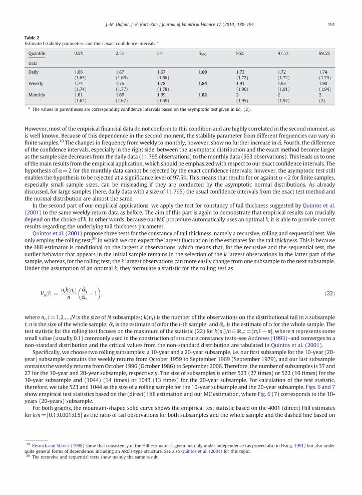
Table 2Estimated stability parameters and their exact confidence intervals. a

Quantile 0.5% 2.5% 5% αMC 95% 97.5% 99.5%

Data

Daily 1.66 1.67 1.67 1.69 1.72 1.72 1.74(1.65) (1.66) (1.66) (1.72) (1.72) (1.73)

Weekly 1.74 1.76 1.78 1.84 1.91 1.93 1.98(1.74) (1.77) (1.78) (1.90) (1.91) (1.94)

Monthly 1.61 1.66 1.69 1.82 2 2 2(1.62) (1.67) (1.69) (1.95) (1.97) (2)

a The values in parentheses are corresponding confidence intervals based on the asymptotic test given in Eq. (2).

19 Resnick and Stâricâ (1998) show that consistency of the Hill estimator is given not only under independence (as proved also in Hsing, 1991) but also undequite general forms of dependence, including an ARCH-type structure. See also Quintos et al. (2001) for this topic.20 The recursive and sequential tests show mainly the same result.

191J.-M. Dufour, J.-R. Kurz-Kim / Journal of Empirical Finance 17 (2010) 180–194

However, most of the empirical financial data do not conform to this condition and are highly correlated in the secondmoment, asis well known. Because of this dependence in the second moment, the stability parameter from different frequencies can vary infinite samples.19 The changes in frequency fromweekly to monthly, however, show no further increase in α. Fourth, the differenceof the confidence intervals, especially in the right side, between the asymptotic distribution and the exact method become largeras the sample size decreases from the daily data (11,795 observations) to themonthly data (563 observations). This leads us to oneof themain results from the empirical application, which should be emphasized with respect to our exact confidence intervals. Thehypothesis of α=2 for the monthly data cannot be rejected by the exact confidence intervals; however, the asymptotic test stillenables the hypothesis to be rejected at a significance level of 97.5%. This means that results for or against α<2 for finite samples,especially small sample sizes, can be misleading if they are conducted by the asymptotic normal distributions. As alreadydiscussed, for large samples (here, daily data with a size of 11,795) the usual confidence intervals from the exact test method andthe normal distribution are almost the same.

In the second part of our empirical applications, we apply the test for constancy of tail thickness suggested by Quintos et al.(2001) to the same weekly return data as before. The aim of this part is again to demonstrate that empirical results can cruciallydepend on the choice of k. In other words, because our MC procedure automatically uses an optimal k, it is able to provide correctresults regarding the underlying tail thickness parameter.

Quintos et al. (2001) propose three tests for the constancy of tail thickness, namely a recursive, rolling and sequential test. Weonly employ the rolling test,20 in which we can expect the largest fluctuation in the estimates for the tail thickness. This is becausethe Hill estimator is conditional on the largest k observations, which means that, for the recursive and the sequential test, theoutlier behavior that appears in the initial sample remains in the selection of the k largest observations in the latter part of thesample, whereas, for the rolling test, the k largest observations canmore easily change from one subsample to the next subsample.Under the assumption of an optimal k, they formulate a statistic for the rolling test as

VnðiÞ =nikðniÞ

nαi

αn� 1

� �; ð22Þ

ni, i=1,2,…,N is the size of N subsamples; k(ni) is the number of the observations on the distributional tail in a subsample

wherei; n is the size of the whole sample; αi is the estimate of α for the i-th sample; and αn is the estimate of α for the whole sample. Thetest statistic for the rolling test focuses on the maximum of the statistic (22) for k(ni)/n∈Rπ:=[π,1−π], where π represents somesmall value (usually 0.1) commonly used in the construction of structure constancy tests–see Andrews (1993)–and converges to anon-standard distribution and the critical values from the non-standard distribution are tabulated in Quintos et al. (2001).

Specifically, we choose two rolling subsamples: a 10-year and a 20-year subsample, i.e. our first subsample for the 10-year (20-year) subsample contains the weekly returns from October 1959 to September 1969 (September 1979), and our last subsamplecontains theweekly returns fromOctober 1996 (October 1986) to September 2006. Therefore, the number of subsamples is 37 and27 for the 10-year and 20-year subsample, respectively. The size of subsamples is either 523 (27 times) or 522 (10 times) for the10-year subsample and (1044) (14 times) or 1043 (13 times) for the 20-year subsample. For calculation of the test statistic,therefore, we take 523 and 1044 as the size of a rolling sample for the 10-year subsample and the 20-year subsample. Figs. 6 and 7show empirical test statistics based on the (direct) Hill estimation and our MC estimation, where Fig. 6 (7) corresponds to the 10-years (20-years) subsample.

For both graphs, the mountain-shaped solid curve shows the empirical test statistic based on the 4001 (direct) Hill estimatesfor k/n=[0.1:0.001:0.5] as the ratio of tail observations for both subsamples and the whole sample and the dashed line based on

r

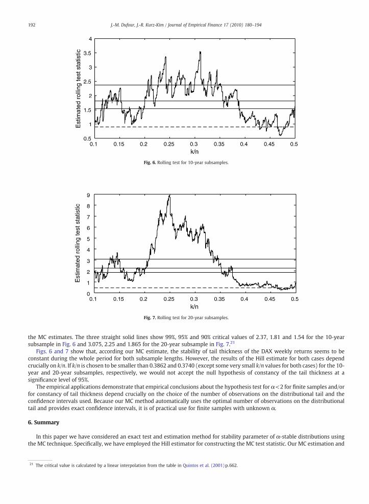
Fig. 7. Rolling test for 20-year subsamples.

21 The critical value is calculated by a linear interpolation from the table in Quintos et al. (2001)p.662.

Fig. 6. Rolling test for 10-year subsamples.

192 J.-M. Dufour, J.-R. Kurz-Kim / Journal of Empirical Finance 17 (2010) 180–194

the MC estimates. The three straight solid lines show 99%, 95% and 90% critical values of 2.37, 1.81 and 1.54 for the 10-yearsubsample in Fig. 6 and 3.075, 2.25 and 1.865 for the 20-year subsample in Fig. 7.21

Figs. 6 and 7 show that, according our MC estimate, the stability of tail thickness of the DAX weekly returns seems to beconstant during the whole period for both subsample lengths. However, the results of the Hill estimate for both cases dependcrucially on k/n. If k/n is chosen to be smaller than 0.3862 and 0.3740 (except some very small k/n values for both cases) for the 10-year and 20-year subsamples, respectively, we would not accept the null hypothesis of constancy of the tail thickness at asignificance level of 95%.

The empirical applications demonstrate that empirical conclusions about the hypothesis test for α<2 for finite samples and/orfor constancy of tail thickness depend crucially on the choice of the number of observations on the distributional tail and theconfidence intervals used. Because our MC method automatically uses the optimal number of observations on the distributionaltail and provides exact confidence intervals, it is of practical use for finite samples with unknown α.

6. Summary

In this paper we have considered an exact test and estimation method for stability parameter of α-stable distributions usingthe MC technique. Specifically, we have employed the Hill estimator for constructing the MC test statistic. Our MC estimation and

193J.-M. Dufour, J.-R. Kurz-Kim / Journal of Empirical Finance 17 (2010) 180–194

test procedure improve on the Hill estimation in twoways: ourMC estimation does not need to assume that the optimal number ofobservations on the distributional tail (or, rather the underlying α) is known, and our MC test provides exact confidence intervalsfor finite samples.

The empirical applications show the sensitive dependency of empirical conclusions on the choice of observations in the tail andthe confidence intervals used, and emphasize the practical meaning of our MC estimation and test procedure.

Acknowledgments

Research support from the Alexander von Humboldt Foundation is gratefully acknowledged by the two authors. Wewould liketo thank three anonymous referees for helpful comments.

Appendix A

Table ARoot mean square error of Hill estimate with different relocations.

α Relocation True mean Sample mean Sample median

Sample size

1.01 100 0.1660 0.3338 0.1654250 0.1235 0.2890 0.1234500 0.0953 0.2697 0.0952

1000 0.0727 0.2711 0.07275000 0.0442 0.1763 0.0442

1.25 100 0.1616 0.2488 0.1625250 0.1063 0.2090 0.1063500 0.0762 0.1845 0.0764

1000 0.0546 0.1771 0.05455000 0.0253 0.1263 0.0253

1.5 100 0.1808 0.1958 0.1813250 0.1126 0.1306 0.1135500 0.0806 0.0949 0.0809

1000 0.0579 0.0761 0.05785000 0.0263 0.0368 0.0262

1.75 100 0.2048 0.2053 0.2068250 0.1291 0.1306 0.1299500 0.0909 0.0912 0.0903

1000 0.0640 0.0655 0.06415000 0.0290 0.0294 0.0290

1.95 100 0.2258 0.2261 0.2259250 0.1421 0.1414 0.1419500 0.0985 0.0987 0.0992

1000 0.0696 0.0698 0.06995000 0.0318 0.0317 0.0317

2.0 100 0.2303 0.2292 0.2313250 0.1463 0.1452 0.1455500 0.1004 0.1010 0.1016

1000 0.0716 0.0714 0.07115000 0.0330 0.0328 0.0327

References

Andrews, D.W.K., 1993. Tests for parameter stability and structural change with unknown change point. Econometrica 59, 817–858.Barnard, G.A., 1963. Comment on “the spectral analysis of point processes” by M.S. Bartlett. Journal of the Royal Statistical Society B 25, 294.Beirlant, J., Vynckier, P., Teugels, J.L., 1996. Tail index estimation, Pareto quantile plots, and regression diagnostics. Journal of the American Statistical Association 91,

1659–1667.Borak, S., Härdle, W., Weron, R., 2005. Stable distributions. In: Cizek, P., Härdle, W., Weron, W. (Eds.), Statistical Tools for Finance and Insurance. Springer Verlag,

Berlin, pp. 21–44.Chambers, J.M., Mallows, C., Stuck, B.W., 1976. A method for simulating stable random variables. Journal of the American Statistical Association 71, 340–344.de Haan, L., Ferreira, A., 2006. Extreme Value Theory, An Introduction. Springer, New York.Deheuvels, P., Häusler, E., Mason, D.M., 1988. Almost sure convergence of the Hill estimator. Mathematical Proceedings of the Cambridge Philosophical Society 104,

372–381.Dekkers, A.L.M., Einmahl, J.H.J., de Haan, L., 1989. A moment estimator for the index of an extreme-value distribution. Annals of Statistics 17, 1833–1855.Dufour, J.-M., 2006. Monte Carlo tests with nuisance parameters: a general approach to finite-sample inference and standard asymptotics in econometrics. Journal

of Econometrics 133, 443–477.Dufour, J.-M., Khalaf, L., Beaulieu, M.-C., 2007. Exact confidence set estimation and goodness-of-fit test methods for asymmetric heavy tailed stable distributions.

Université Laval. Manuscript.DuMouchel, W.H., 1971. Stable distributions in statistical inference, Ph.D. Thesis, Yale University.DuMouchel, W.H., 1983. Estimating the stable index α in order to measure tail thickness: a critique. Annals of Statistics 11, 1019–1031.

194 J.-M. Dufour, J.-R. Kurz-Kim / Journal of Empirical Finance 17 (2010) 180–194

Dwass, M., 1957. Modified randomization tests for nonparametric hypotheses. Annals of Mathematical Statistics 28, 181–187.Fama, E.F., French, K.R., 1992. The cross-section of expected stock returns. Journal of Finance 47, 427–465.Goldie, C.M., Smith, R.L., 1987. Slow variation with remainder: a survey of the theory and its applications. Quarterly Journal of Mathematics Oxford 38, 45–71.Hill, B.M., 1975. A simple general approach to inference about the tail of a distribution. Annals of Statistics 3, 1163–1174.Hodges Jr., J.L., Lehmann, E.L., 1963. Estimates of location based on rank tests. The Annals of Mathematical Statistics 34, 598–611.Hsing, T., 1991. On tail index estimation using dependent data. Annals of Statistics 19, 1547–1569.Huisman, R., Koedijk, K.G., Kool, C.J.M., Palm, F., 2001. Tail-index estimates in small samples. Journal of Business & Economic Statistics 19, 208–216.Kim, J.-R., Mittnik, S., Rachev, S.T., 1997. Detecting asymmetries in observed time series and unobserved disturbances. Studies in Nonlinear Dynamics and

Econometrics 1, 131–143.Kurz-Kim, J.-R., Loretan, M., 2007. A note on the coefficient of determination in models with infinite-variance variable. International Finance Discussion Paper 895,

Board of Governors of the Federal Reserve System.Mandelbrot, B., 1963. The variation of certain speculative prices. Journal of Business 36, 394–419.Mason, D.M., 1982. Laws of large numbers for sums of extreme values. Annals of Probability 10, 756–764.McCulloch, J.H., 1986. Simple consistent estimators of stable distribution parameters. Communications in Statistics, Computation and Simulation 15, 1109–1136.McCulloch, J.H., 1996. Financial applications of stable distributions. In: Maddala, G.S., Rao, C.R. (Eds.), Handbook of Statistics — Statistical Methods in Finance,

vol. 14. Elsevier Science B.V, Amsterdam, pp. 393–425.McCulloch, J.H., 1997. Measuring tail thickness to estimate the stable index α: a critique. Journal of Business and Economic Statistics 15, 74–81.McCulloch, J.H., 1998. Linear regression with stable disturbances. In: Adler, R., Feldman, R., Taqqu, M.S. (Eds.), A Practical Guide to Heavy Tails: Statistical

Techniques for Analysing Heavy Tailed distributions. Birkhäuser, Boston, pp. 359–376.Pickands, J., 1975. Statistical inference using extreme order statistics. Annals of Statistics 3, 119–131.Quintos, C., Fan, Z., Phillips, P.C.B., 2001. Structural change tests in tail behaviour and the Asian crisis. Review of Economic Studies 68, 633–663.Rachev, S.T., Mittnik, S., 2000. Stable Paretian Models in Finance. John Wiley & Sons, Chichester.Rachev, S.T., Kim, J.-R., Mittnik, S., 1999. Stable Paretian econometrics part I and II. The Mathematical Scientists 24, 24–55 and 113–127.Reiss, H.D., 1989. Approximate Distributions of Order Statistics with Applications to Nonparametric Statistics. Springer Series in Statistics, Springer-Verlag, New York.Resnick, S., Stâricâ, C., 1998. Tail index estimation for dependent data. Annals of Applied Probability 8, 1156–1183.Samorodnitsky, G., Taqqu, M.S., 1994. Stable Non-Gaussian Random Processes. Chapman & Hall, New York.Segers, J., 2002. Abelian and Tauberian Theorems on the bias of the Hill estimator. Scandinavian Journal of Statistics 29, 461–483.Zolotarev, V.M., 1986. One-Dimensional Stable Distributions. Translations of Mathematical Monographs, vol. 65. American Mathematical Society. Providence.